

Water Structure in the Utrish Nature Reserve (Black Sea) during 2020–2021 According to Thermistor Chain Data

 ,
,  ,
,
Abstract
1. Introduction
2. Materials and Methods
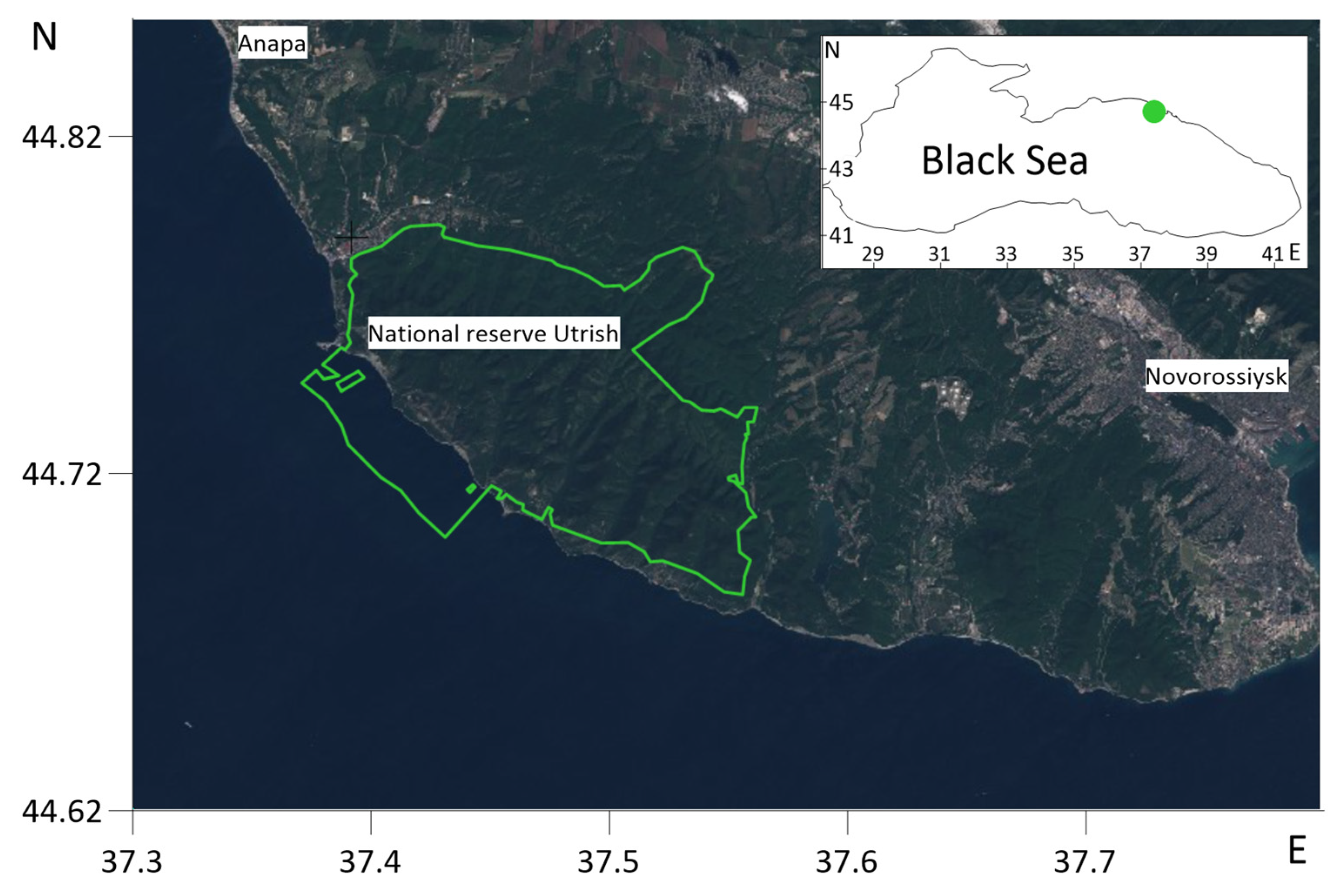
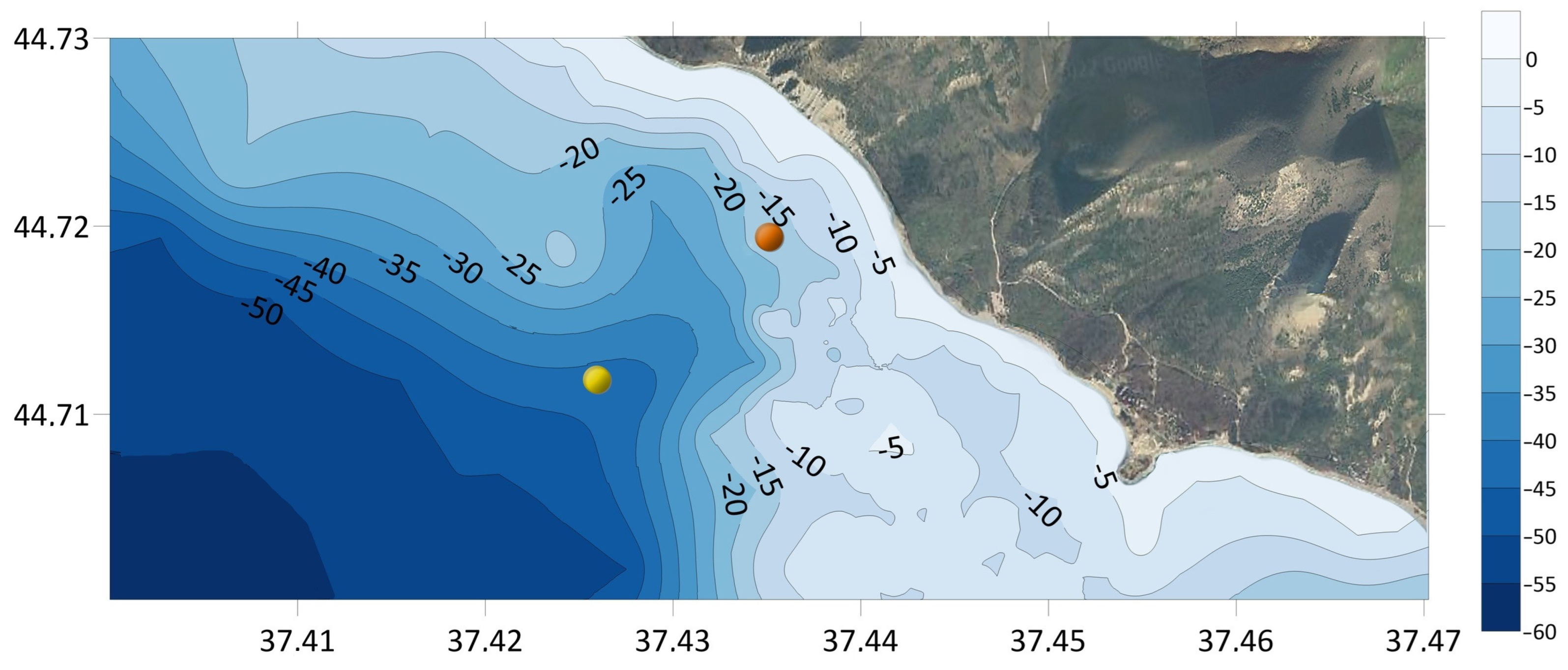
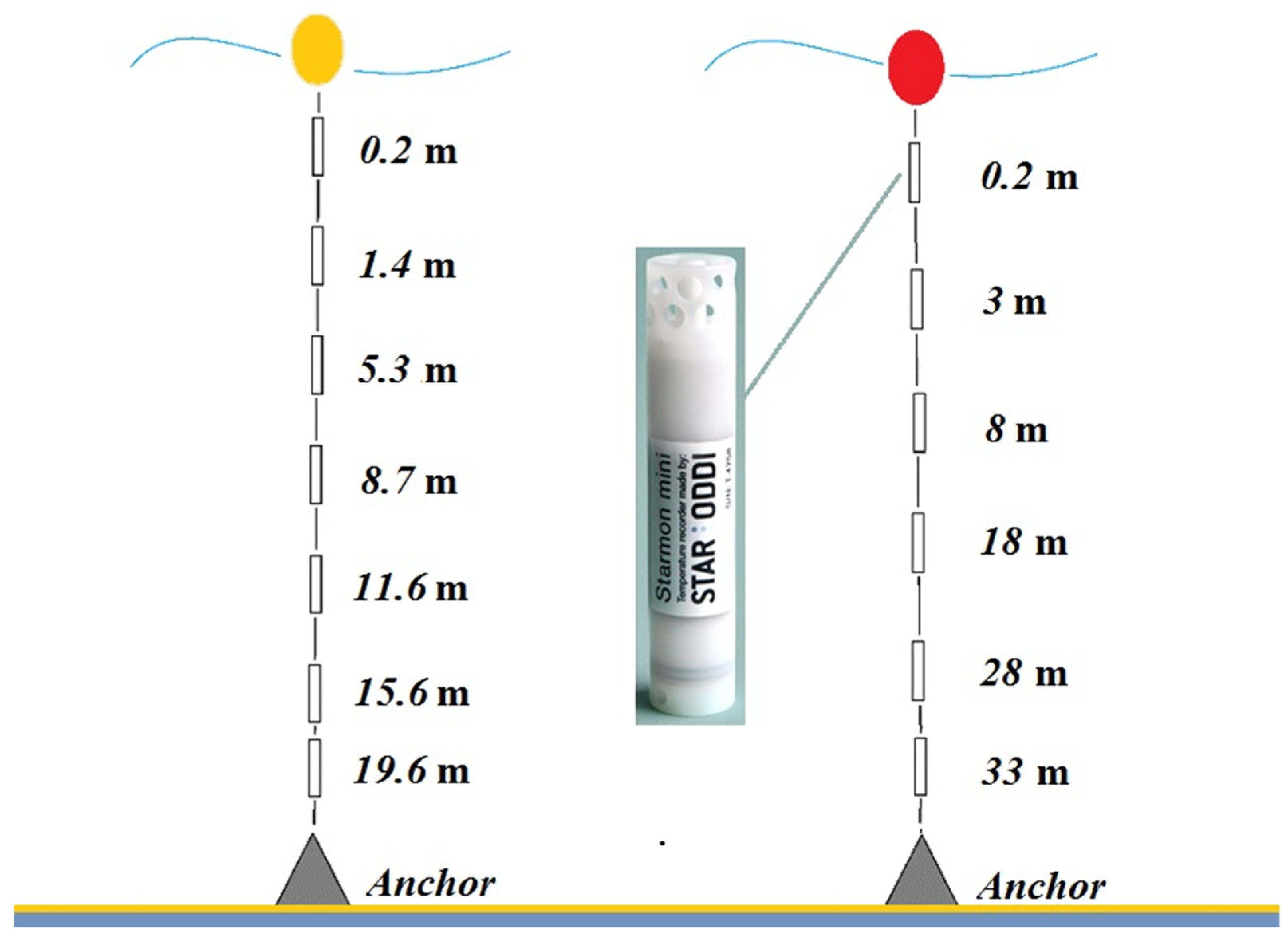
2.1. In Situ Thermistor Chain Data
2.2. Methods
2.3. Model Description
3. Results and Discussion
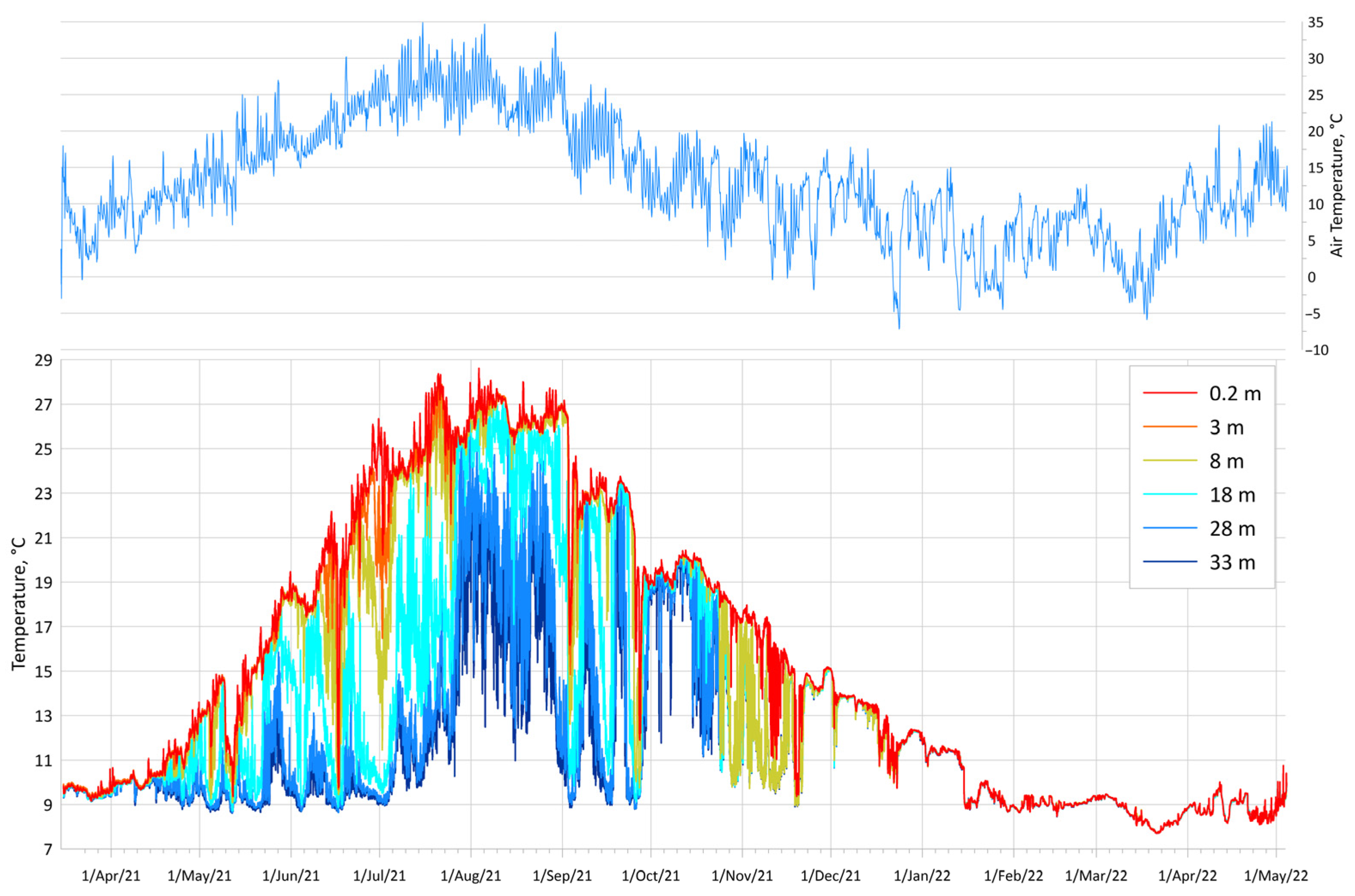
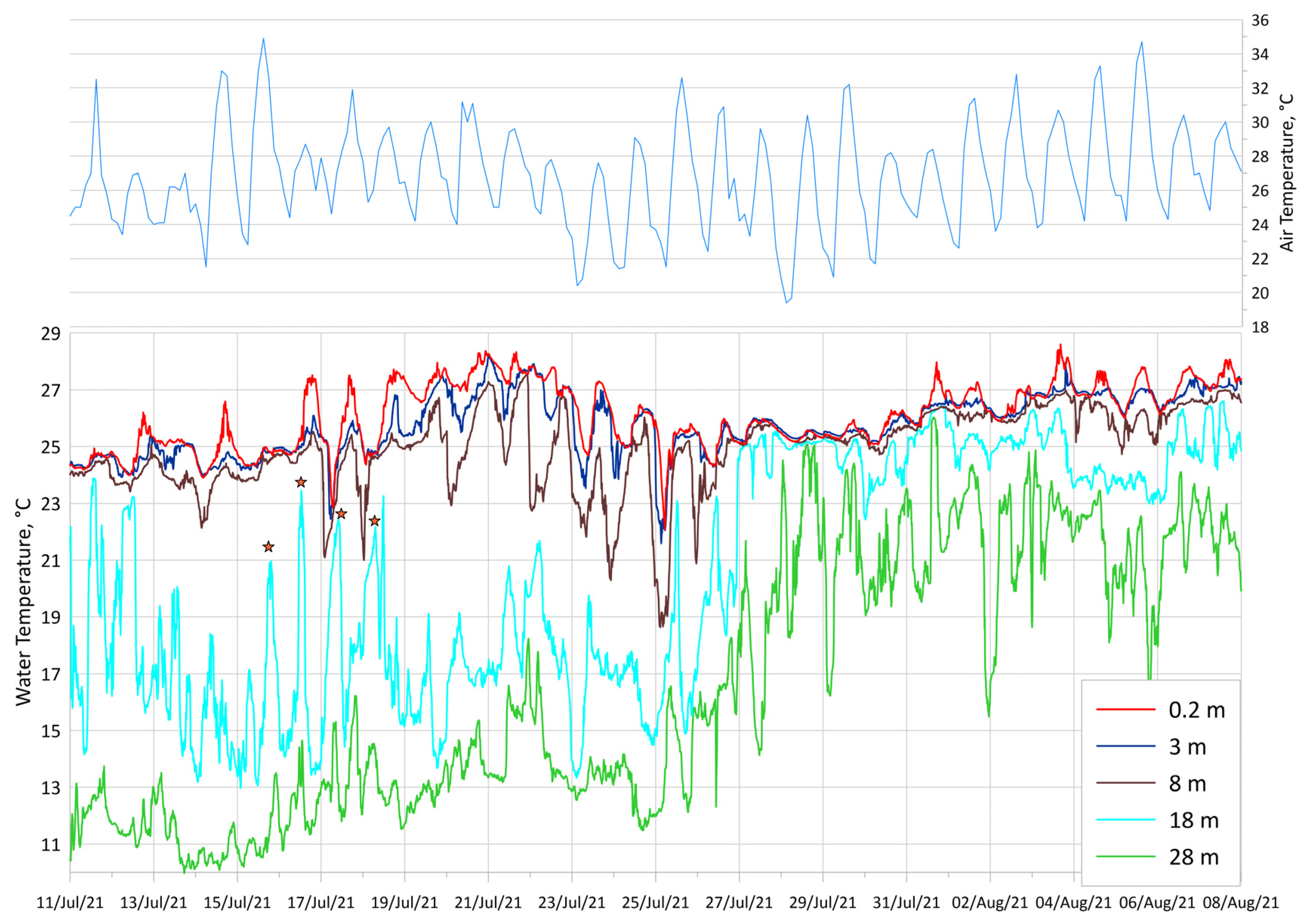
3.1. General Description
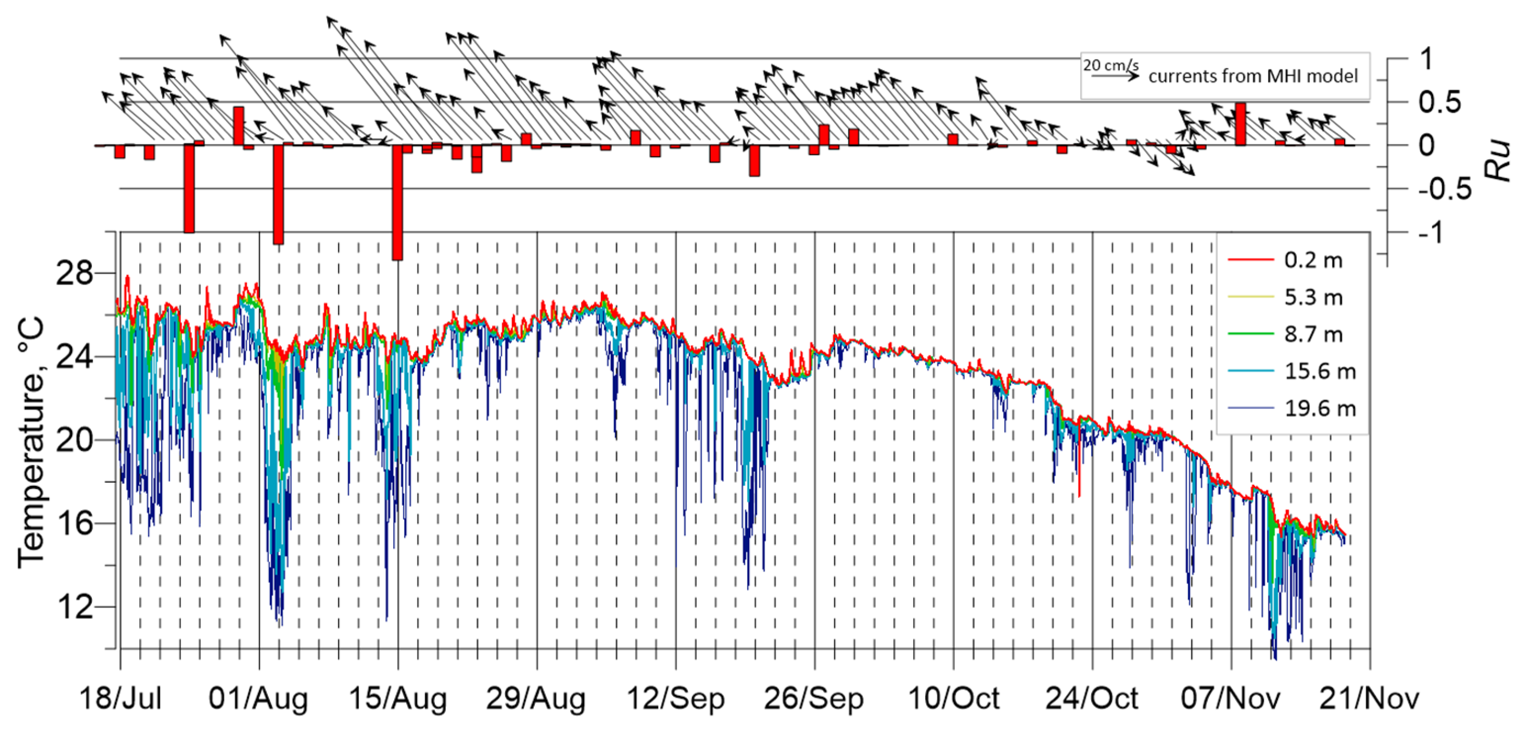
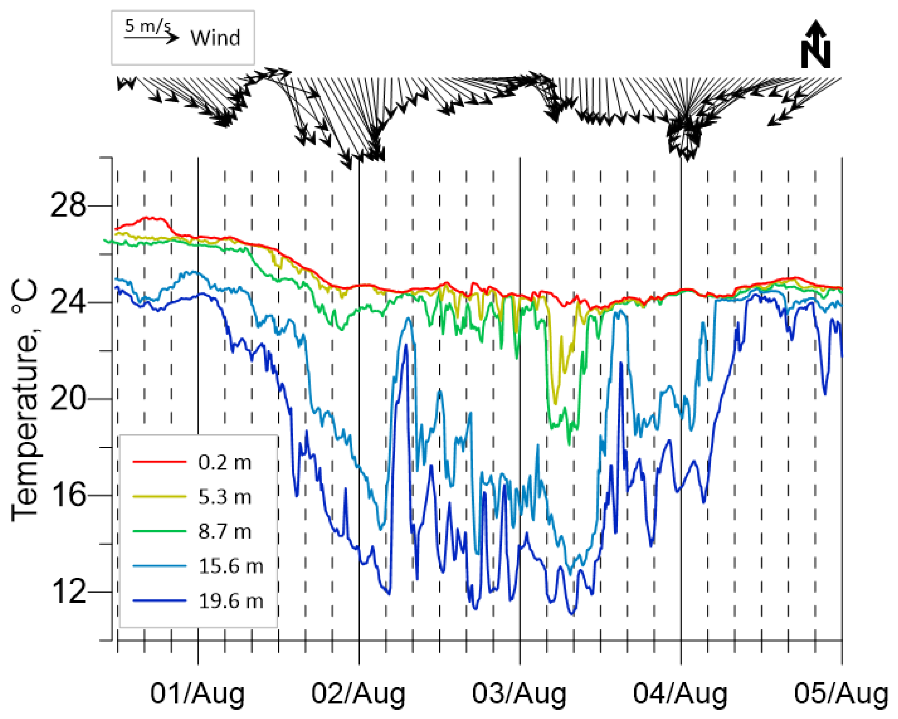
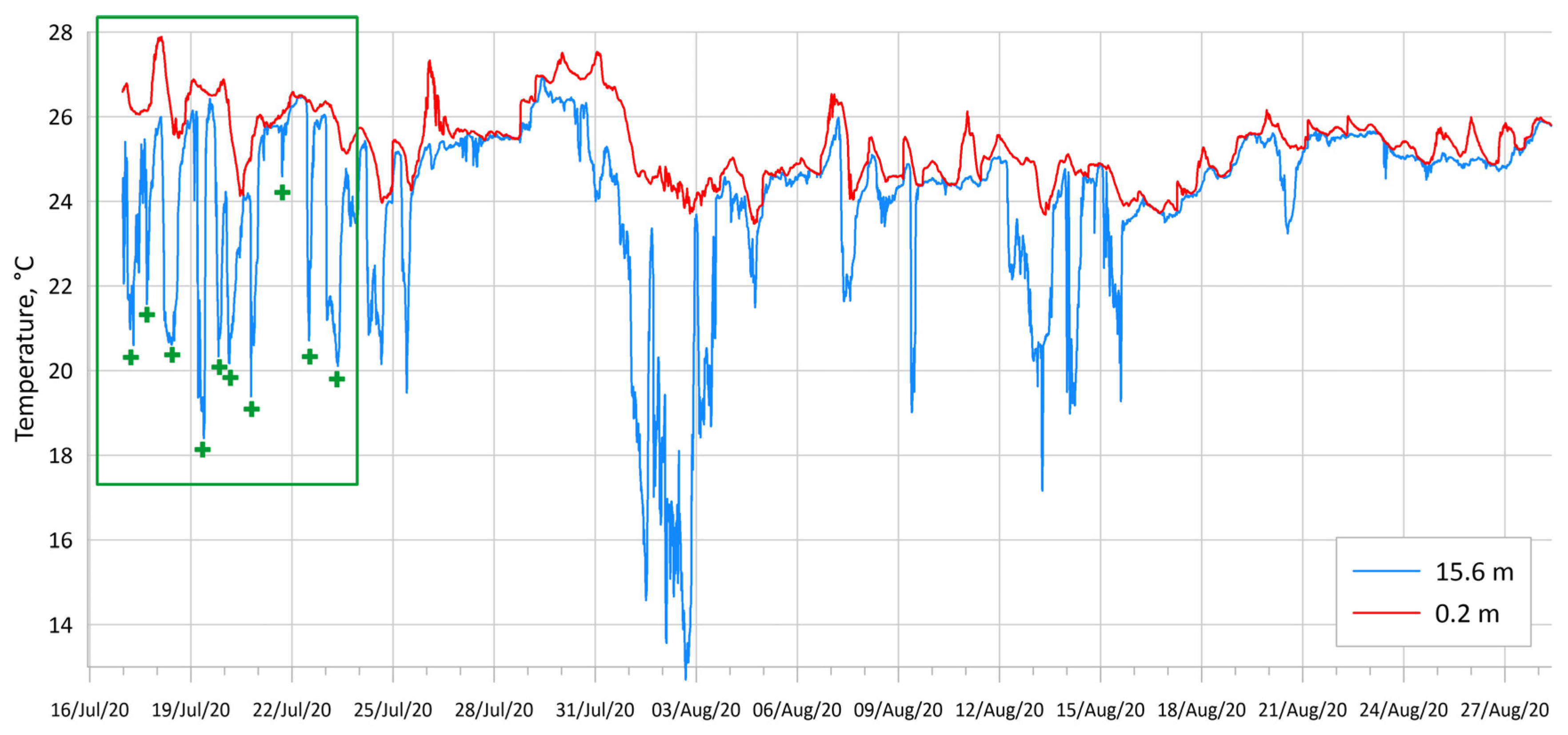
3.2. Upwelling Events during Measurement Periods
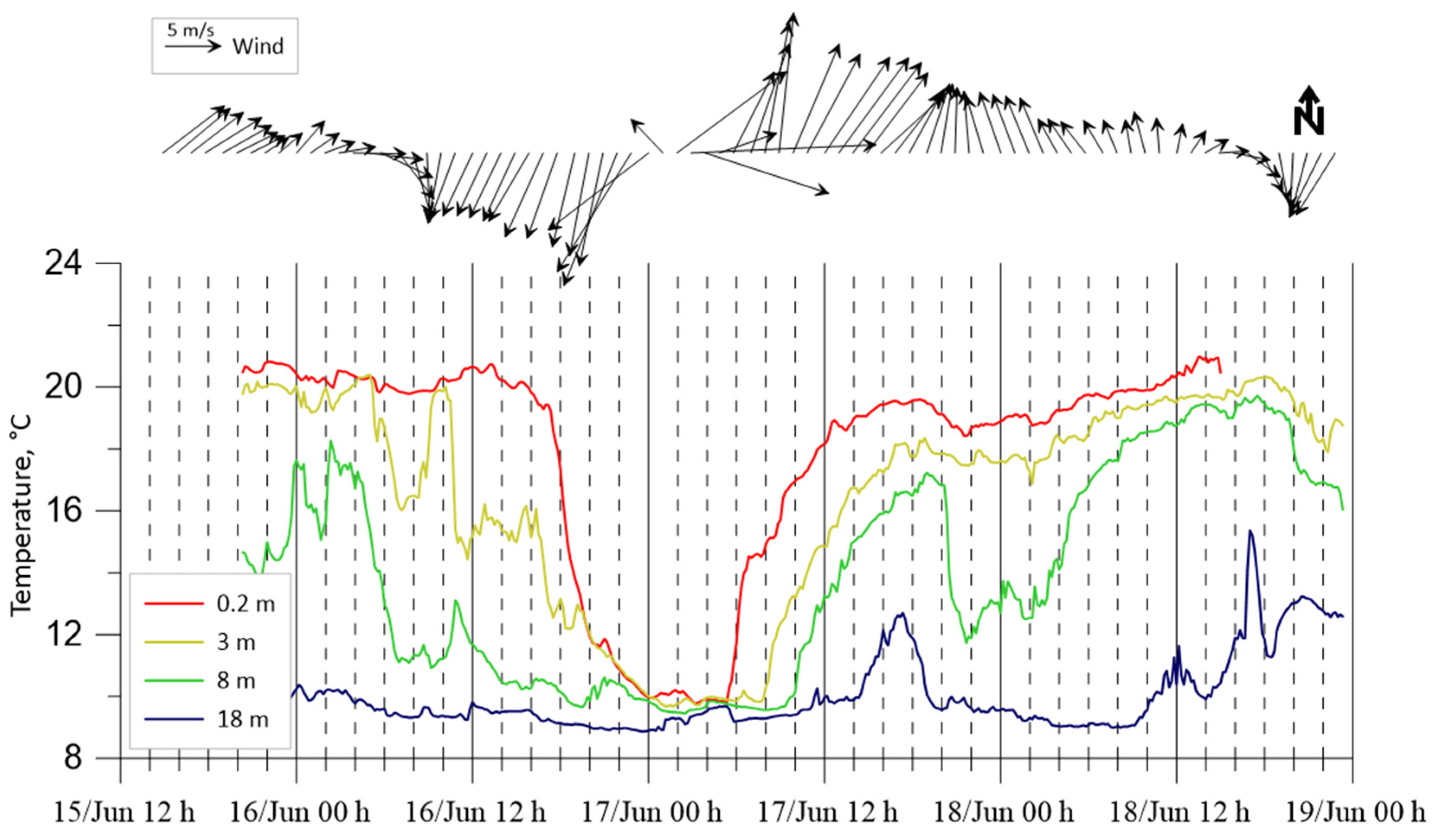
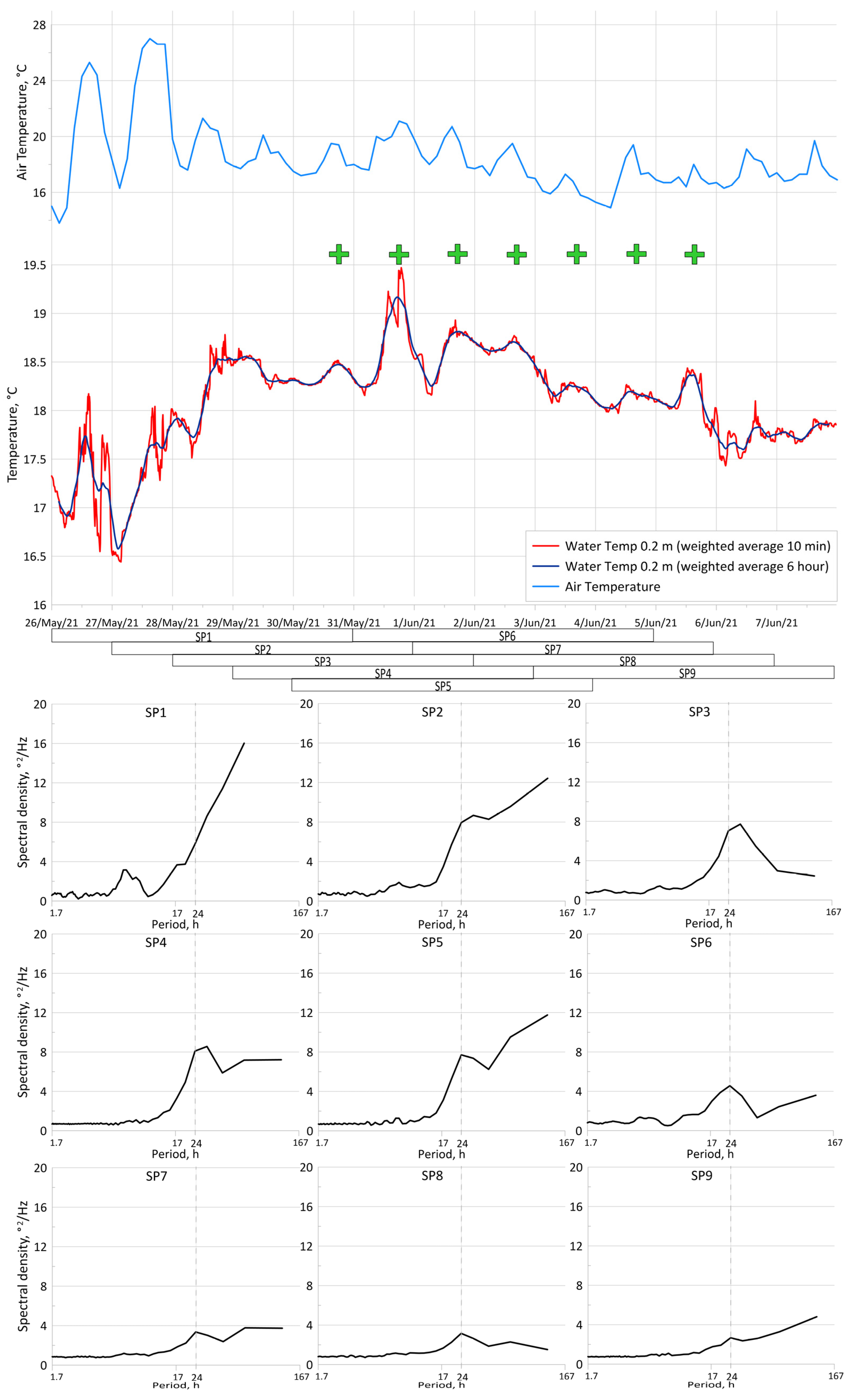
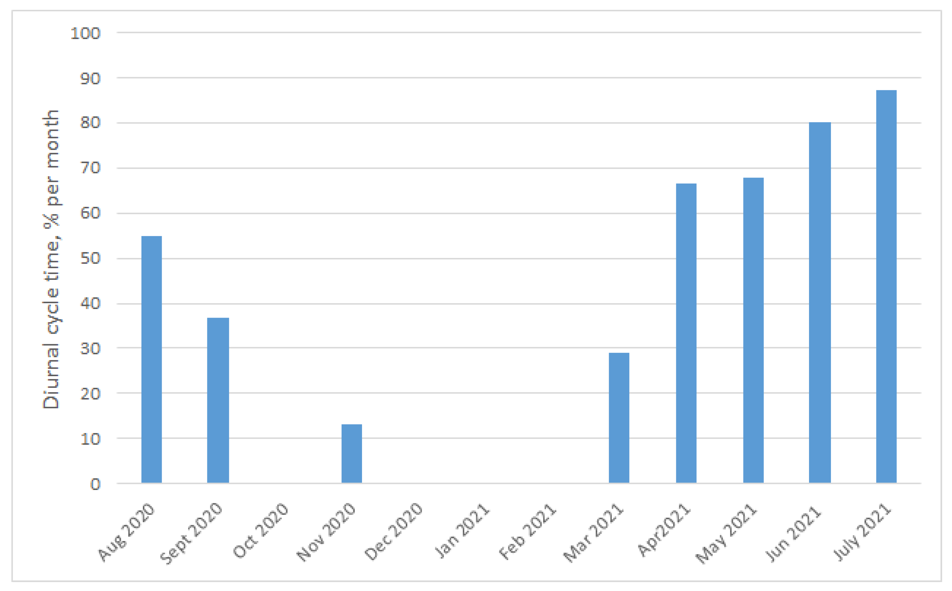
3.3. Diurnal Cycle
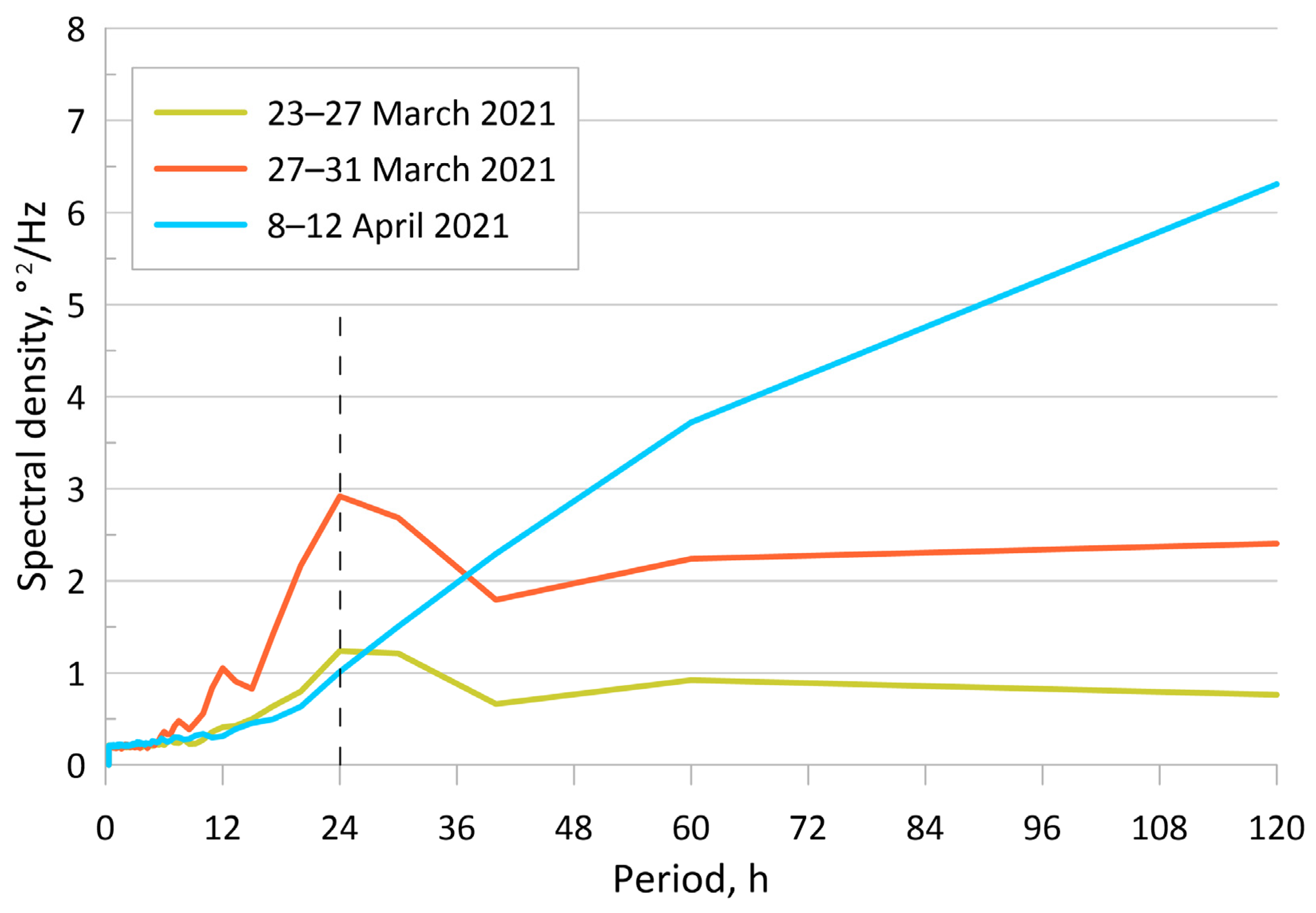
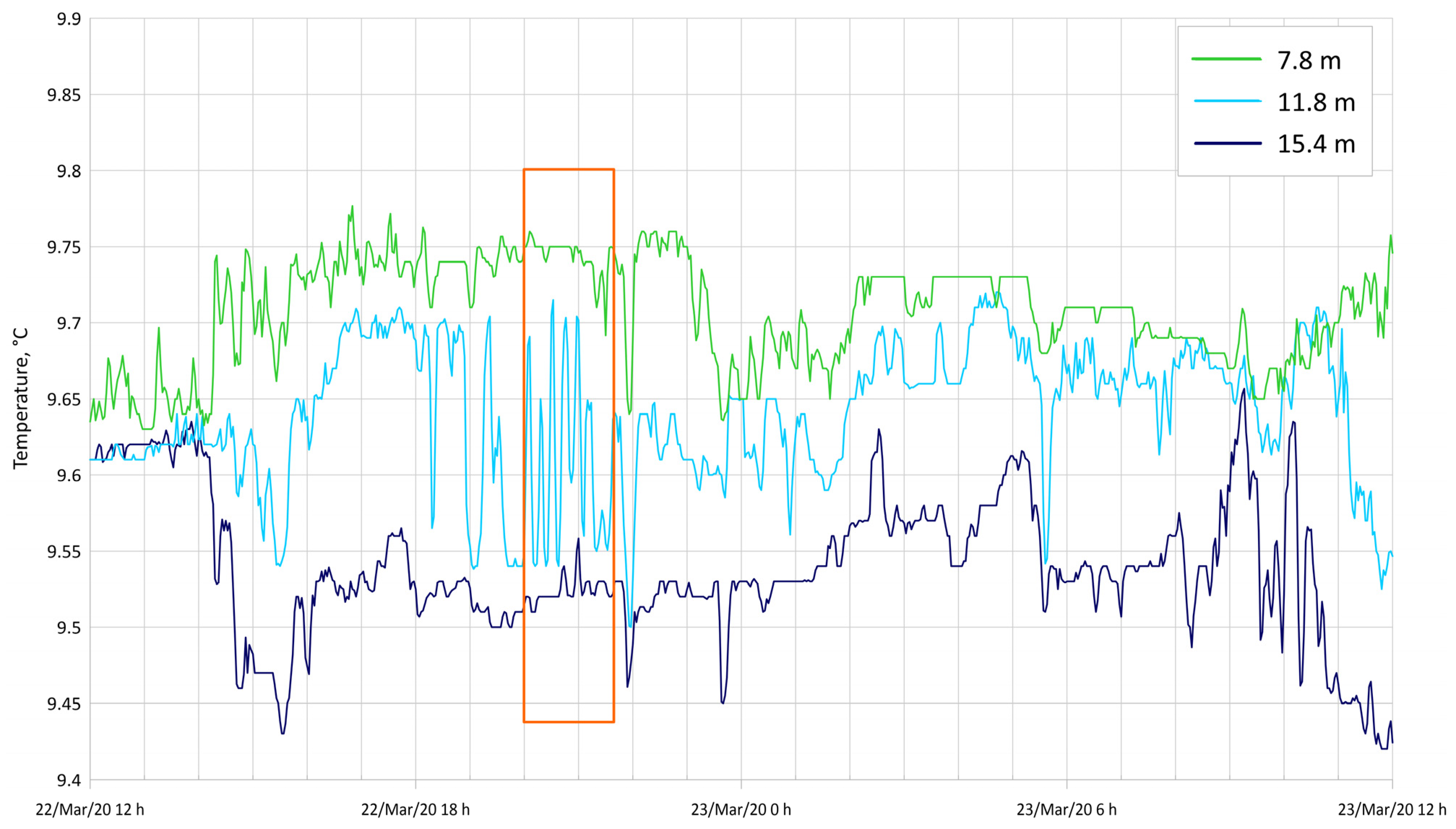
3.4. Internal Waves
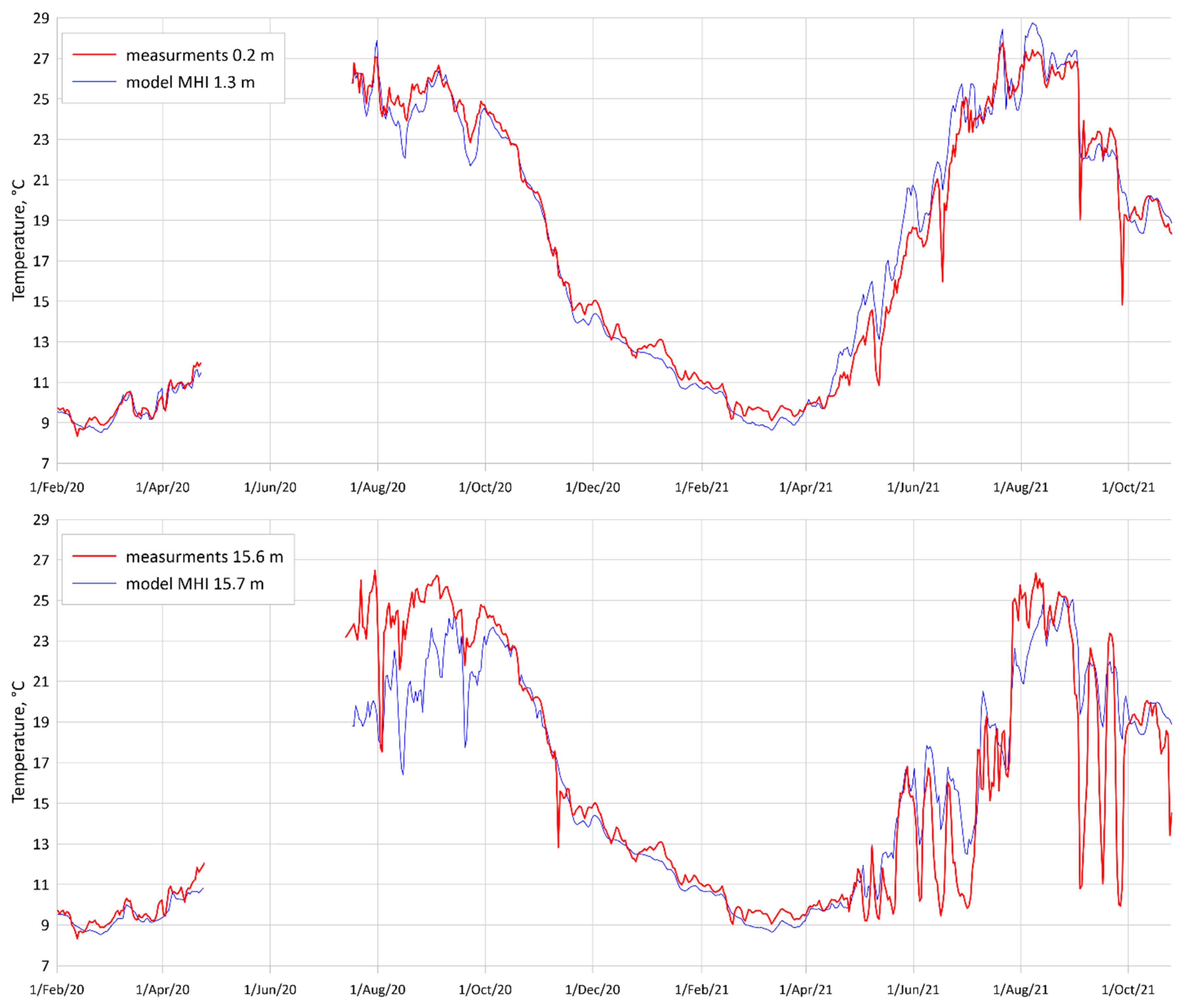
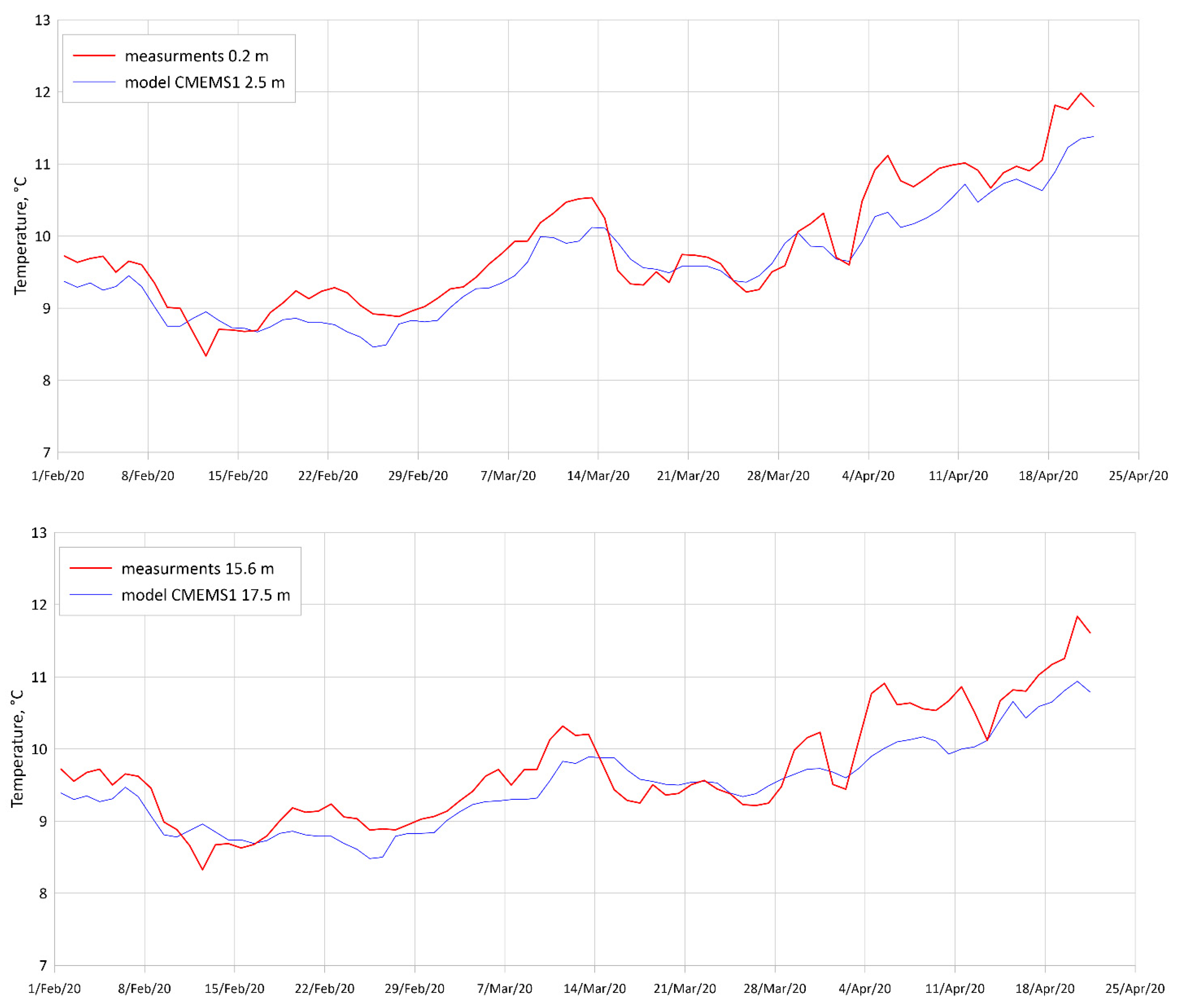
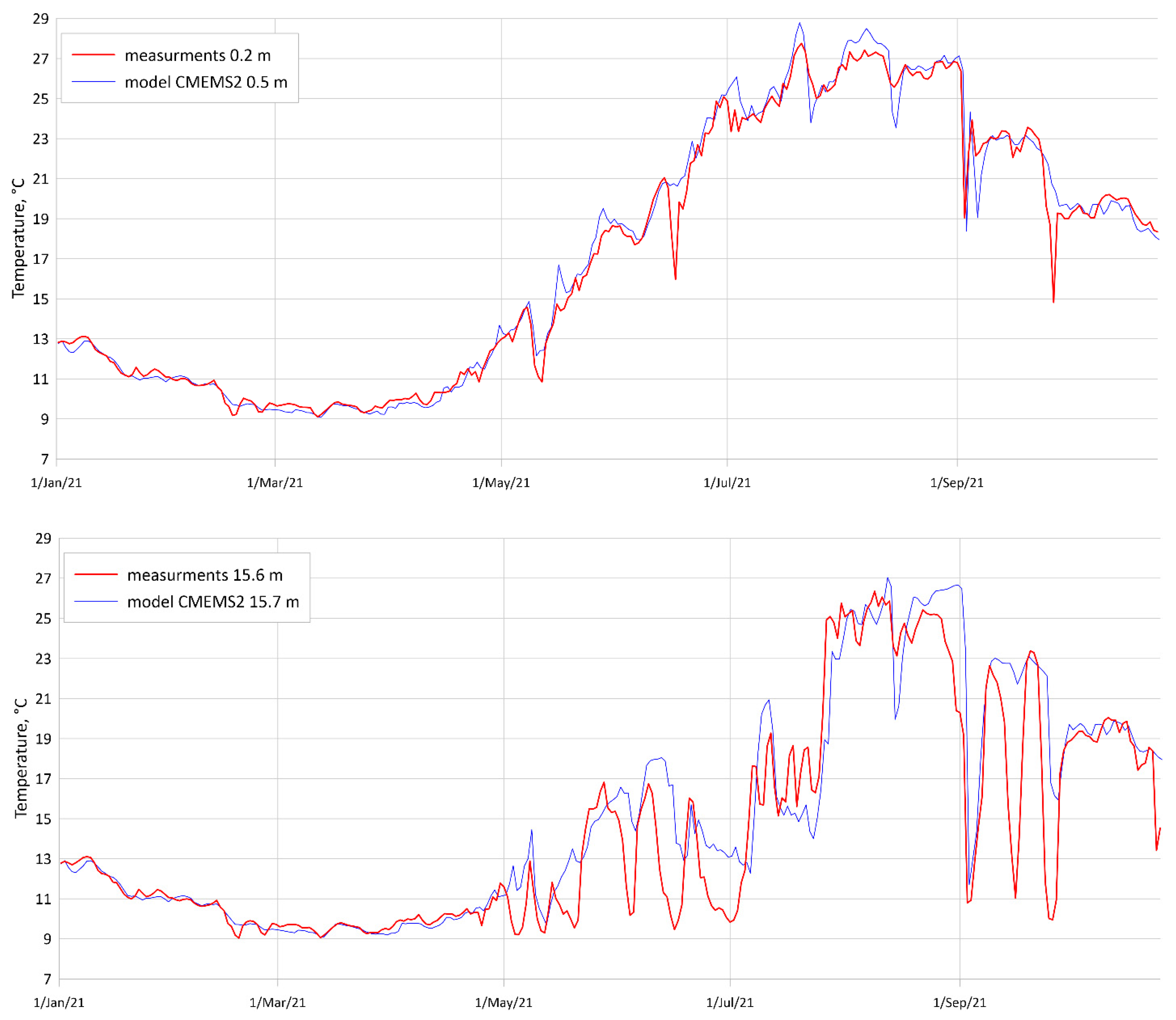
3.5. Model Quality Assessment
4. Summary and Conclusions
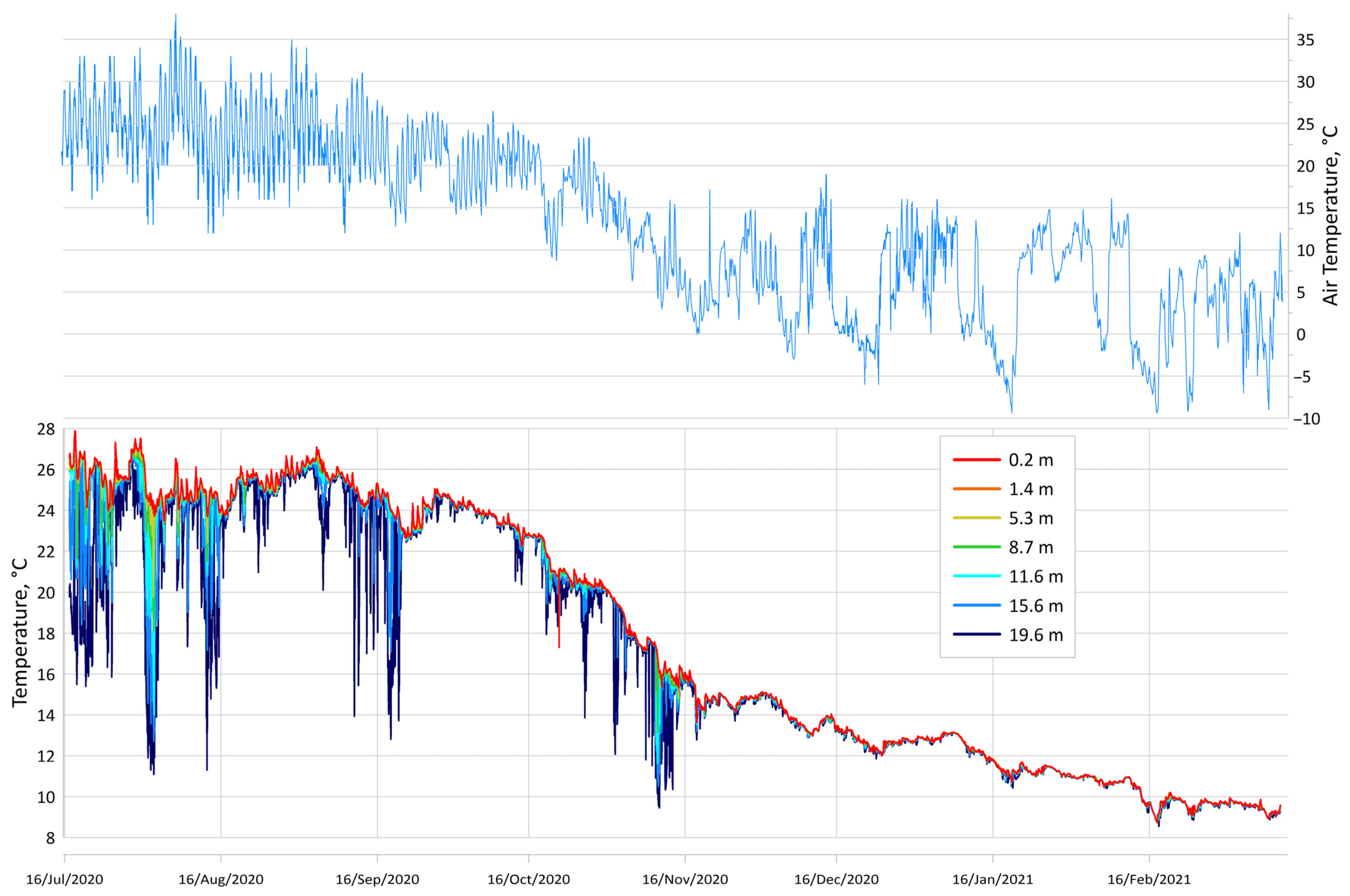
- A unique series of long-term water temperature data for Utrish was obtained and processed for the first time. Seasonal fluctuations in the water temperature could have a range from 8 °C in February to 28 °C in August. The characteristics of the temperature variability during the year in the NR Utrish water area are a valuable result for further ecosystem studies.
- The diurnal cycle of water temperature was observed mainly in the spring–autumn period. According to the analysis, daytime heating usually does not exceed 2 °C. Internal waves could also affect the temperature structure, but their influence is momentary.
- Short-period fluctuations in the temperature associated with an upwelling were greater than 10 °C. The water temperature decreased from 28 °C to 17 °C in a very short time—6–12 h. Evidence of such strong variations is essential for benthic communities’ studies. Upwelling in the Black Sea could lead to the vertical oscillation of the hypoxic layer, significantly affecting benthic communities [82].
- High-resolution simulation data were compared with in situ data. SST is more precise than subsurface temperature, and the RMSE for all model SSTs was less than 1 °C. Thus, modern hydrodynamic models could be used for climatological and seasonal research in the studied area, but extreme short-term events were reproduced badly.
- In situ measurements of the temperature verified the temperature structure in the coastal area of the Black Sea and provided support for all further ecosystem studies in the NR Utrish.
Author Contributions
Funding
Institutional Review Board Statement
Informed Consent Statement
Acknowledgments
Conflicts of Interest
References
- NR Utrish. Available online: https://utrishgpz.ru/about (accessed on 21 March 2023).
- Kolyuchkina, G.A.; Syomin, V.; Simakova, U.; Mokievsky, V.O. Presentability of the Utrish Nature Reserve’s benthic communities for the North Caucasian Black Sea Coast. Nat. Conserv. Res. 2018, 3, 1–16. [Google Scholar] [CrossRef]
- Glazov, D.M.; Bykhalova, O.N.; Udovik, D.A.; Yu, G.; Pilipenko, K.K.; Tarasiyan, V.V. Rozhnov Seasonal occurrence and distribution of whales in the Utrish reserve and adjacent sea waters. In Terrestrial and Marine Ecosystems of the Abrau Peninsula: History, Condition, Protection, Place of Publication Anapa; Bykhalova, O.N., Ed.; 2021; Volume 5, pp. 249–262. (In Russian) [Google Scholar]
- Ecological Atlas. Black and Azov Seas/Rosneft Oil Company PJSC, Arctic Science Center LLC, Research Foundation; NIR Foundation: Moscow, Russia, 2019; 464p. (In Russian) [Google Scholar]
- Pearson, T.H.; Rosenberg, R. Feast and famine: Structuring factors in marine benthic communities. In Organization of Communities: Past and Present; Gee, J.H.R., Giller, P.S., Eds.; Blackwell Science: Oxford, UK, 1987; pp. 373–395. [Google Scholar]
- Kolyuchkina, G.A.; Syomin, V.L.; Grigorenko, K.S.; Basin, A.B.; Lyubimov, I.V. The Role of Abiotic Environmental Factors in the Vertical Distribution of Macrozoobenthos at the Northeastern Black Sea Coast. Biol. Bull. 2020, 47, 1126–1141. [Google Scholar] [CrossRef]
- Vershinin, A.O.; Moruchkov, A.A.; Sukhanova, I.N.; Kamnev, A.N.; Morton, S.L.; Ramsdell, J.S.; Pan’kov, S.L. Seasonal changes in phytoplankton in the area of Cape Bolshoi Utrish off the Northern Caucasian coast in the Black Sea, 2001–2002. Oceanology 2004, 44, 372–378. [Google Scholar]
- Alimov, A.F. Intensity of metabolism in aquatic poikilothermic animals. In General Principles for the Study of Aquatic Ecosystems; Nauka: Leningrad, Russia, 1979; pp. 1–20. (In Russian) [Google Scholar]
- Kubryakov, A.; Bagaev, A.; Stanichny, S.; Belokopytov, V. Thermohaline structure, transport and evolution of the Black Sea eddies from hydrological and satellite data. Prog. Oceanogr. 2018, 167, 44–63. [Google Scholar] [CrossRef]
- Akpinar, A.; Fach, B.A.; Oguz, T. Observing the subsurface thermal signature of the Black Sea Cold Intermediate Layer with Argo profiling floats. Deep. Sea Res. Part I Oceanogr. Res. Pap. 2017, 124, 140–142. [Google Scholar] [CrossRef]
- Tuzhilkin, V.S.; Arkhipkin, V.S.; Myslenkov, S.A.; Sam-borsky, T.V. Synoptic variability of thermohalineconditions in the Russian part of the Black Sea coastal zone. Vestnik Moskovskogo Universiteta, Ser. 5. Geography 2012, 6, 46–53. [Google Scholar]
- Podymov, O.I.; Zatsepin, A.G.; Ocherednik, V.V. Increase of Temperature and Salinity in the Active Layer of the North-Eastern Black Sea from 2010 to 2020. Phys. Oceanogr. 2021, 28, 257–265. [Google Scholar] [CrossRef]
- Ivanov, V.A.; Belokopytov, V.N. Oceanography of the Black Sea; Marine Hydrophysical Inst., National Academy of Sciences of Ukraine: Sevastopol, Russia, 2011. (In Russian)
- Shapiro, G. Black Sea Circulation. In Encyclopedia of Ocean Sciences; Academic Press: Cambridge, MA, USA, 2010; pp. 401–414. [Google Scholar] [CrossRef]
- Staneva, J.V.; Dietrich, D.E.; Stanev, E.V.; Bowman, M.J. Rim Current and coastal eddy mechanisms in aneddy-resolving Black Sea general circulation model. J. Mar. Syst. 2001, 31, 137–157. [Google Scholar] [CrossRef]
- Kubryakov, A.A.; Stanichny, S.V.; Zatsepin, A.G.; Kremenetskiy, V.V. Long-term variations of the Black Sea dynamics and their impact on the marine ecosystem. J. Mar. Syst. 2016, 163, 80–94. [Google Scholar] [CrossRef]
- Kubryakov, A.A.; Stanichny, S.V. Mesoscale eddies in the Black Sea from satellite altimetry data. Oceanology 2015, 55, 56–67. [Google Scholar] [CrossRef]
- Zatsepin, A.G.; Ginzburg, A.I.; Kostianoy, A.G.; Kremenetskiy, V.; Krivosheya, V.G.; Stanichny, S.; Poulain, P.-M. Observations of Black Sea mesoscale eddies and associated horizontal mixing. J. Geophys. Res. 2003, 108, 3246. [Google Scholar] [CrossRef]
- Zatsepin, A.G.; Baranov, V.I.; Kondrashov, A.A.; Korzh, A.O.; Kremenetskiy, V.V.; Ostrovskii, A.G.; Soloviev, D.M. Submesoscale eddies at the caucasus Black Sea shelf and the mechanisms of their generation. Oceanology 2011, 51, 554. [Google Scholar] [CrossRef]
- Miladinova, S.; Stips, A.; Garcia-Gorriz, E.; Moy, D.M. Black Sea thermohaline properties: Long-term trends and variations. J. Geophys. Res. Oceans 2017, 122, 5624–5644. [Google Scholar] [CrossRef] [PubMed]
- Mohamed, B.; Ibrahim, O.; Nagy, H. Sea Surface Temperature Variability and Marine Heatwaves in the Black Sea. Remote Sens. 2022, 14, 2383. [Google Scholar] [CrossRef]
- Ginzburg, A.I.; Kostianoy, A.G.; Serykh, I.V.; Lebedev, S.A. Climate Change in the Hydrometeorological Parameters of the Black and Azov Seas (1980–2020). Oceanology 2021, 61, 745–756. [Google Scholar] [CrossRef]
- Ivanov, V.A.; Mikhailova, É.N. Upwelling in the Black Sea; ÉKOSI-Gidrofizika: Sevastopol, Russia, 2008. (In Russian) [Google Scholar]
- Stanichnaya, R.R.; Sergey, S. Black Sea upwellings. Sovrem. Probl. Distantsionnogo Zondirovaniya Zemli Iz Kosm. 2021, 18, 195–207. [Google Scholar] [CrossRef]
- Polonskii, A.; Muzyleva, M.A. Modern spatial-temporal variability of upwelling in the North-Western Black Sea and off the Crimea Coast. Izv. Ross. Akad. Nauk. Seriya Geogr. 2016, 4, 96–108. [Google Scholar] [CrossRef]
- Gawarkiewicz, G.; Korotaev, G.; Stanichny, S.; Repetin, L.; Soloviev, D. Synoptic upwelling and cross-shelf transport processes along the Crimean coast of the Black Sea. Cont. Shelf Res. 1999, 19, 977–1005. [Google Scholar] [CrossRef]
- Lomakin, P.D. Upwelling in the Kerch Strait and the adjacent waters of the Black Sea basedon the contact and satellite data. Morskoy Gidrofiz. Zhurnal 2018, 34, 123–133. [Google Scholar] [CrossRef]
- Silvestrova, K.P.; Zatsepin, A.G.; Myslenkov, S.A. Coastal upwelling in the Gelendzhik area of the Black Sea: Effect of wind and dynamics. Oceanology 2017, 57, 469–477. [Google Scholar] [CrossRef]
- Novikov, A.A.; Tuzhilkin, V.S. Seasonal and regionalvariations of water temperature synoptic anomalies in thenortheastern coastal zone of the Black Sea. Phys. Oceanogr. 2015, 1, 39–48. [Google Scholar]
- Divinsky, B.V.; Kuklev, S.B.; Zatsepin, A.G. Numerical simulation of an intensive upwelling event in the northeastern part of the Black Sea at the IO RAS hydrophysical testing site. Oceanology 2017, 57, 615–620. (In Russian) [Google Scholar] [CrossRef]
- Zatsepin, A.G.; Ostrovskii, A.G.; Kremenetskiy, V.V.; Nizov, S.S.; Piotoukh, V.B.; Soloviev, V.A.; Shvoev, D.A.; Tsibul’sky, A.L.; Kuklev, S.B.; Moskalenko, L.V.; et al. Subsatellite Polygon for Studying Hydrophysical Processes in the Black Sea Shelf–Slope Zone. Izv. Atmos. Ocean. Phys. 2014, 50, 16–29. [Google Scholar] [CrossRef]
- Ostrovskii, A.G.; Zatsepin, A.G.; Soloviev, V.A.; Tsibulsky, A.L.; Shvoev, D.A. Autonomous System for Vertical Profiling of the Marine Environment at a Moored Station. Oceanology 2013, 53, 233–242. [Google Scholar] [CrossRef]
- Ocherednik, V.V.; Baranov, V.I.; Zatsepin, A.G.; Kyklev, S.B. Thermochains of the Southern Branch, Shirshov Institute of Oceanology, Russian Academy of Sciences: Design, Methods, and Results of Metrological Investigations of Sensors. Oceanology 2018, 58, 661–671. [Google Scholar] [CrossRef]
- Ocherednik, V.V.; Zatsepin, A.G.; Kuklev, S.B.; Baranov, V.I.; Mashura, V.V. Examples of Approaches to Studying the Temperature Variability of Black Sea Shelf Waters with a Cluster of Temperature Sensor Chains. Oceanology 2020, 60, 149–160. [Google Scholar] [CrossRef]
- Ostrovskii, A.G.; Emelianov, M.V.; Kochetov, O.Y.; Kremenetskiy, V.V.; Shvoev, D.A.; Volkov, S.V.; Zatsepin, A.G.; Korovchinsky, N.M.; Olshanskiy, V.M.; Olchev, A.V. Automated Tethered Profiler for Hydrophysical and Bio-Optical Measurements in the Black Sea Carbon Observational Site. J. Mar. Sci. Eng. 2022, 10, 322. [Google Scholar] [CrossRef]
- Zatsepin, A.G.; Podymov, O.I. Thermohaline Anomalies and Fronts in the Black Sea and Their Relationship with the Vertical Fine Structure. Oceanology 2021, 61, 757–768. [Google Scholar] [CrossRef]
- Baranov, V.I.; Ocherednik, V.V.; Zatsepin, A.G.; Kuklev, S.B.; Mashura, V.V. First Results of Using an Automatic Stationary Station for Vertical Profiling of Aquatic Media at the Gelendzhik Research Site: A Promising Tool for Real-Time Coastal Oceanography. Oceanology 2020, 60, 120–126. [Google Scholar] [CrossRef]
- Kuklev, S.B.; Zatsepin, A.G.; Paka, V.T.; Baranov, V.I.; Kukleva, O.N.; Podymov, O.I.; Podufalov, A.P.; Korg, A.O.; Kondrashov, A.A.; Soloviev, D.M. Experience of Simultaneous Measurements of Parameters of Currents and Hydrological Structure of Water from a Moving Vessel. Oceanology 2021, 61, 132–138. [Google Scholar] [CrossRef]
- Tolstosheev, A.P.; Motyzhev, S.V.; Lunev, E.G. Results of Long-Term Monitoring of the Shelf Water Vertical Thermal Struture at the Black Sea Hydrophysical Polygon of RAS. Phys. Oceanogr. 2020, 27, 69–80. [Google Scholar] [CrossRef]
- Serebryany, A.N.; Khimchenko, E.E. Internal Waves of Mode 2 in the Black Sea. Dokl. Earth Sci. 2019, 488, 1227–1230. [Google Scholar] [CrossRef]
- Serebryany, A.; Khimchenko, E.; Zamshin, V.; Popov, O. Features of the Field of Internal Waves on the Abkhazian Shelf of the Black Sea according to Remote Sensing Data and In Situ Measurements. J. Mar. Sci. Eng. 2022, 10, 1342. [Google Scholar] [CrossRef]
- Korshenko, E.A.; Diansky, N.A.; Fomin, V.V. Reconstruction of the Black Sea Deep-Water Circulation Using INMOM and Comparison of the Results with the ARGO Buoys Data. Morskoy Gidrofiz. Zhurnal 2019, 35, 220–232. (In Russian) [Google Scholar] [CrossRef]
- Arkhipkin, V.S.; Kosarev, A.N.; Gippius, F.N.; Migali, D.I. Seasonal variability of the climatic fields of temperature, salinity and circulation of the Black and Caspian seas. Mosc. Univ. Bull. Ser. 5 Geogr. 2013, 5, 33–44. (In Russian) [Google Scholar]
- Stanev, E. Understanding Black Sea Dynamics: Overview of Recent Numerical Modeling. Oceanography 2005, 18, 56–75. [Google Scholar] [CrossRef]
- Demyshev, S.G.; Dymova, O.A.; Markova, N.V.; Korshenko, E.A.; Senderov, M.V.; Turko, N.A.; Ushakov, K.V. Undercurrents in the Northeastern Black Sea Detected on the Basis of Multi-Model Experiments and Observations. J. Mar. Sci. Eng. 2021, 9, 933. [Google Scholar] [CrossRef]
- Diansky, N.A.; Fomin, V.V.; Grigoriev, A.V.; Chaplygin, A.V.; Zatsepin, A.G. Spatial-temporal variability of inertial currents in the eastern part of the Black Sea in a storm period. Phys. Oceanogr. 2019, 26, 135–146. [Google Scholar] [CrossRef]
- Gusev, A.V.; Zalesny, V.B.; Fomin, V.V. Technique for Simulation of Black Sea Circulation with Increased Resolution in the Area of the IO RAS Polygon. Oceanology 2017, 57, 880–891. [Google Scholar] [CrossRef]
- Korotaev, G.K.; Shutyaev, V.P. Numerical Simulation of Ocean Circulation with Ultrahigh Spatial Resolution. Izv. Atmos. Ocean. Phys. 2020, 56, 289–299. [Google Scholar] [CrossRef]
- Palazov, A.; Ciliberti, S.; Peneva, E.; Gregoire, M.; Staneva, J.; Lemieux-Dudon, B.; Masina, S.; Pinardi, N.; Vandenbulcke, L.; Behrens, A.; et al. Black Sea Observing System. Front. Mar. Sci. 2019, 6, 315. [Google Scholar] [CrossRef]
- Ciliberti, S.A.; Grégoire, M.; Staneva, J.; Palazov, A.; Coppini, G.; Lecci, R.; Peneva, E.; Matreata, M.; Marinova, V.; Masina, S.; et al. Monitoring and Forecasting the Ocean State and Biogeochemical Processes in the Black Sea: Recent Developments in the Copernicus Marine Service. J. Mar. Sci. Eng. 2021, 9, 1146. [Google Scholar] [CrossRef]
- Korotaev, G.K.; Knysh, V.V.; Kubryakov, A.I. Study of formation process of cold intermediate layer based on reanalysis of Black Sea hydrophysical fields for 1971–1993. Izv. Atmos. Ocean. Phys. 2014, 50, 35–48. [Google Scholar] [CrossRef]
- Lima, L.; Aydoğdu, A.; Escudier, R.; Masina, S.; Ciliberti, S.A.; Azevedo, D.; Peneva, E.L.; Causio, S.; Cipollone, A.; Clementi, E.; et al. Black Sea Physical Reanalysis (CMEMS BS-Currents) (Version 1) [Data Set]; Copernicus Monitoring Environment Marine Service (CMEMS): Ramonville-Saint-Agne, France, 2020; Available online: https://resources.marine.copernicus.eu/product-detail/BLKSEA_MULTIYEAR_PHY_007_004/INFORMATION (accessed on 15 August 2021). [CrossRef]
- Gunduz, M.; Özsoy, E.; Hordoir, R. A model of Black Sea circulation with strait exchange (2008–2018). Geosci. Model Dev. 2020, 13, 121–138. [Google Scholar] [CrossRef]
- Demyshev, S.G.; Dymova, O.A. Numerical analysis of the Black Sea currents and mesoscale eddies in 2006 and 2011. Ocean. Dyn. 2018, 68, 1335–1352. [Google Scholar] [CrossRef]
- Mizyuk, A.I.; Korotaev, G.K. Black Sea intrapycnocline lenses according to the results of a numerical simulation of basin circulation. Izv. Atmos. Ocean. Phys. 2020, 56, 92–100. [Google Scholar] [CrossRef]
- Kholod, A.L.; Ratner, Y.B.; Ivanchik, M.V.; Martinov, M.V. Estimation of the numerical modeling accuracy of the Black Sea thermohaline fields based on using ARGO profiling floats. J. Phys.: Conf. Ser. 2018, 1128, 012150. [Google Scholar] [CrossRef]
- Lima, L.; Ciliberti, S.; Aydogdu, A.; Escudier, R.; Masina, S.; Azevedo, D.; Peneva, E.; Causio, S.; Cipollone, A.; Clementi, E.; et al. Quality Information Document CMEMS. 2022. Available online: https://catalogue.marine.copernicus.eu/documents/QUID/CMEMS-BS-QUID-007-004.pdf (accessed on 21 March 2023).
- Myslenkov, S.; Silvestrova, K.; Krechik, V.; Kapustina, M. Verification of the Ekman Upwelling Criterion with In Situ Temperature Measurements in the Southeastern Baltic Sea. J. Mar. Sci. Eng. 2023, 11, 179. [Google Scholar] [CrossRef]
- Krechik, V.; Myslenkov, S.; Kapustina, M. New possibilities in the study of coastal upwellings in the southeastern Baltic Sea with using thermistor chain. Geogr. Environ. Sustain. 2019, 12, 44–61. [Google Scholar] [CrossRef]
- Saha, S.; Moorthi, S.; Wu, X.; Wang, J.; Nadiga, S.; Tripp, P.; Behringer, D.; Hou, Y.-T.; Chuang, H.-Y.; Iredell, M.; et al. The NCEP climate forecast system version 2. J. Clim. 2014, 27, 2185–2208. [Google Scholar] [CrossRef]
- Available online: https://rp5.ru/ (accessed on 21 March 2023).
- Petrov, D. Properties of the frequency spectra of the temperature anomalies of ocean surface and near-surface air in a simple stochastic climate model with fluctuating parameters. Извecтия Poccийcкoй Aкaдeмии Hayк. Физикa Aтмocфepы u Oкeaнa 2019, 55, 27–36. [Google Scholar] [CrossRef]
- Khosravi, Y.; Bahri, A.; Tavakoli, A. Spectral Analysis of Spatial Relationship between Surface Wind Speed (SWS) and Sea Surface Temperature (SST) in Oman Sea. Phys. Geogr. Res. Q. 2018, 50, 473–489. [Google Scholar] [CrossRef]
- NEMO Ocean Engine; NEMO System Team. Scientific Notes of Climate Modelling Center, 27; Institute Pierre-Simon Laplace (IPSL): Guyancourt, France, 2022. [Google Scholar] [CrossRef]
- Mizyuk, A.I.; Korotaev, G.K.; Grigoriev, A.V.; Puzina, O.S.; Lishaev, P.N. Long-Term Variability of Thermohaline Characteristics of the Azov Sea Based on the Numerical Eddy-Resolving Model. Phys. Oceanogr. 2019, 26, 438–450. [Google Scholar] [CrossRef]
- EMODnet Bathymetry Consortium. EMODnet Digital Bathymetry (DTM 2016); EMODnet Bathymetry Consortium: Brussels, Belgium, 2020. [Google Scholar] [CrossRef]
- Large, W.G.; Yeager, S. Diurnal to Decadal Global Forcing for Ocean and Sea-Ice Models: The Data Sets and Flux Climatologies (No. NCAR/TN-460+STR); National Center of Atmospheric Research: Boulder, CO, USA, 2004. [Google Scholar] [CrossRef]
- Mulet, S.; Rio, M.-H.; Mignot, A.; Guinehut, S.; Morrow, R. A new estimate of the global 3D geostrophic ocean circulation based on satellite data and in-situ measurements. Deep. Sea Res. Part II Top. Stud. Oceanogr. 2012, 77, 70–81. [Google Scholar] [CrossRef]
- Dobricic, S.; Pinardi, N. An oceanographic three-dimensional variational data assimilation scheme. Ocean. Model. 2008, 22, 89–105. [Google Scholar] [CrossRef]
- Storto, A.; Dobricic, S.; Masina, S.; Di Pietro, P. Assimilating along-track altimetric observations through local hydrostatic adjustment in a global ocean variational assimilation system. Mon. Wea. Rev. 2011, 139, 738–754. [Google Scholar] [CrossRef]
- Jansen, E.; Martins, D.; Stefanizzi, L.; Ciliberti, S.A.; Gunduz, M.; Ilicak, M.; Lecci, R.; Cretí, S.; Causio, S.; Aydoğdu, A.; et al. BLKSEA_ANALYSISFORECAST_PHY_007_001, Black Sea Physical Analysis and Forecast (Copernicus Marine Service BS-Currents, EAS5 system) (Version 1) Data Set; Copernicus Monitoring Environment Marine Service (CMEMS): Ramonville-Saint-Agne, France, 2022. [Google Scholar] [CrossRef]
- Belokopytov, V.N. Interannual variations of the renewal of waters of the cold intermediate layer in the Black Sea for the last decades. Phys. Oceanogr. 2011, 20, 347–355. [Google Scholar] [CrossRef]
- Miladinova, S.; Stips, A.; Garcia-Gorriz, E.; Moy, D.M. Formation and changes of the Black Sea cold intermediate layer. Prog. Oceanogr. 2018, 167, 11–23. [Google Scholar] [CrossRef]
- Silvestrova, K.; Myslenkov, S.; Zatsepin, A. Variability of wind-driven coastal upwelling in the north-eastern Black Sea in 1979–2016 according to NCEP/CFSR data. Pure Appl. Geophys. 2018, 175, 4007–4015. [Google Scholar] [CrossRef]
- Zatsepin, A.G.; Silvestrova, K.P.; Kuklev, S.B.; Piotoukh, V.B.; Podymov, O.I. Observations of a cycle of intense coastal upwelling and downwelling at the research site of the Shirshov Institute of Oceanology in the Black Sea. Oceanology 2016, 56, 188–199. [Google Scholar] [CrossRef]
- Rubakina, V.A.; Kubryakov, A.A.; Stanichny, S.V. Seasonal and diurnal cycle of the Black Sea water temperature from temperature-profiling drifters data. Sovrem. Probl. Distantsionnogo Zondirovaniya Zemli Iz Kosm. 2019, 16, 268–281. [Google Scholar] [CrossRef]
- Ivanov, V.A.; Shul’ga, T.Y.; Bagaev, A.V.; Medvedeva, A.V.; Plastun, T.V.; Verzhevskaya, L.V.; Svishcheva, I.A. Internal Waves on the Black Sea Shelf near the Heracles Peninsula: Modeling and Observation. Morskoy Gidrofiz. Zhurnal 2019, 35, 322–340. [Google Scholar] [CrossRef]
- Ivanova, I.; Shlychkov, V. Internal Waves on the Black Sea Shelf. Bull. Russ. Acad. Sci. Phys. 2018, 82, 1573–1576. [Google Scholar] [CrossRef]
- Serebryany, A.; Khimchenko, E.; Popov, O.; Denisov, D.; Kenigsberger, G. Internal Waves Study on a Narrow Steep Shelf of the Black Sea Using the Spatial Antenna of Line Temperature Sensors. J. Mar. Sci. Eng. 2020, 8, 833. [Google Scholar] [CrossRef]
- Khimchenko, E.; Ostrovskii, A.; Klyuvitkin, A.; Piterbarg, L. Seasonal Variability of Near-Inertial Internal Waves in the Deep Central Part of the Black Sea. J. Mar. Sci. Eng. 2022, 10, 557. [Google Scholar] [CrossRef]
- Mizyuk, A. Numerical Modelling: Report; Marine Hydrophysical Institute: Sevastopol, Russia, 2022; pp. 1–47. (In Russian) [Google Scholar]
- Kolyuchkina, G.A.; Syomin, V.L.; Simakova, U.V.; Sergeeva, N.G.; Ananiev, R.A.; Dmitrevsky, N.N.; Ostrovskii, A.G. Benthic community structure near the margin of the oxic zone: A case study on the Black Sea. J. Mar. Syst. 2022, 227, 103691. [Google Scholar] [CrossRef]


| Thermistor Depth, m | Average Temp | Median Temp | Minimum Temp | Maximum Temp | Standard Deviation | Variation Coefficient | Comments |
|---|---|---|---|---|---|---|---|
| 0.2 | 9.81 | 9.63 | 8.14 | 12.99 | 0.84 | 0.09 | |
| 2.5 | 9.82 | 9.63 | 8.15 | 12.90 | 0.83 | 0.08 | |
| 3.8 | 9.78 | 9.60 | 8.14 | 12.40 | 0.81 | 0.08 | |
| 5.9 | 9.28 | 9.23 | 8.14 | 10.52 | 0.48 | 0.05 | Worked till 11 March 2020 |
| 7.8 | 9.40 | 9.37 | 8.13 | 10.61 | 0.49 | 0.05 | Worked till 1 April 2020 |
| 9.7 | 9.73 | 9.57 | 8.14 | 12.23 | 0.78 | 0.08 | |
| 11.8 | 9.71 | 9.54 | 8.12 | 12.06 | 0.77 | 0.08 | |
| 13.8 | 9.70 | 9.52 | 8.12 | 12.04 | 0.76 | 0.08 | |
| 15.4 | 9.68 | 9.51 | 8.13 | 12.04 | 0.75 | 0.08 |
| Thermistor Depth, m | Average Temp | Median Temp | Minimum Temp | Maximum Temp | Standard Deviation | Variation Coefficient | Comments |
|---|---|---|---|---|---|---|---|
| 0.2 | 17.85 | 15.97 | 8.73 | 27.88 | 6.23 | 0.35 | |
| 1.4 | 20.37 | 22.88 | 12.10 | 27.75 | 5.21 | 0.26 | Worked till 14 January 2021 |
| 5.3 | 17.81 | 15.94 | 8.75 | 27.07 | 6.19 | 0.35 | |
| 8.7 | 17.76 | 15.87 | 8.75 | 26.98 | 6.15 | 0.35 | |
| 11.6 | 17.67 | 15.72 | 8.73 | 26.95 | 6.10 | 0.35 | |
| 15.6 | 17.47 | 15.47 | 8.74 | 26.92 | 5.98 | 0.34 | |
| 19.6 | 16.97 | 14.91 | 8.54 | 26.83 | 5.72 | 0.34 |
| Thermistor Depth | Average Temp | Median Temp | Minimum Temp | Maximum Temp | Standard Deviation | Variation Coefficient | Comments |
|---|---|---|---|---|---|---|---|
| 0.2 | 19.20 | 19.71 | 9.16 | 28.60 | 5.99 | 0.31 | |
| 3 | 18.64 | 18.80 | 9.26 | 28.19 | 6.41 | 0.34 | |
| 8 | 18.21 | 18.78 | 9.09 | 27.54 | 5.85 | 0.32 | |
| 18 | 15.58 | 14.63 | 8.71 | 27.08 | 5.59 | 0.36 | |
| 28 | 13.06 | 10.70 | 8.63 | 26.02 | 4.48 | 0.34 | |
| 33 | 12.33 | 10.17 | 8.61 | 25.14 | 3.91 | 0.32 | |
| Bottom (33 m) | 11.01 | 9.39 | 7.70 | 18.57 | 2.87 | 0.26 | 25 October 2021–4 May 2022 |
| Model | Depth Model, m/Depth Measurement | Period | Sample | R Correlation | Bias (Model-Measurement) | RMSE |
|---|---|---|---|---|---|---|
| MHI | 1.3/0.2 | 1 February 2020– 25 October 2021 | 545 | 0.99 | 0.03 | 0.91 |
| MHI | 15.7/15.6 | 1 February 2020– 25 October 2021 | 545 | 0.93 | −0.23 | 2.23 |
| CMEMS1 | 2.5/0.2 | 1 February 2020– 21 April 2020 | 81 | 0.95 | −0.24 | 0.37 |
| CMEMS1 | 17.5/15.6 | 1 February 2020– 21 April 2020 | 81 | 0.92 | −0.22 | 0.38 |
| CMEMS2 | 0.5/0.2 | 1 January 2021– 25 October 2021 | 296 | 0.99 | 0.17 | 0.79 |
| CMEMS2 | 15.7/15.6 | 1 January 2021– 25 October 2021 | 296 | 0.92 | 0.74 | 2.22 |
| Model | Depth Model, m/Depth Measurement | Bias (Model-Measurement) | RMSE (Root Mean Square Error) |
|---|---|---|---|
| CMEMS1 | SST | 0.14 | 0.59 |
| CMEMS1 | 5–10 | −0.096 | 1.09 |
| CMEMS1 | 10–20 | −0.048 | 1.82 |
| CMEMS2 | SST | 0.080 | 0.330 |
| CMEMS2 | 0–10 | 0.006 | 0.593 |
| CMEMS2 | 10–100 | −0.031 | 0.634 |
| Layer, m | Bias, °C | RMSE, °C |
|---|---|---|
| 0.0–5.0 | 0.096 | 0.675 |
| 5.0–30.0 | −0.182 | 1.515 |
Disclaimer/Publisher’s Note: The statements, opinions and data contained in all publications are solely those of the individual author(s) and contributor(s) and not of MDPI and/or the editor(s). MDPI and/or the editor(s) disclaim responsibility for any injury to people or property resulting from any ideas, methods, instructions or products referred to in the content. |
© 2023 by the authors. Licensee MDPI, Basel, Switzerland. This article is an open access article distributed under the terms and conditions of the Creative Commons Attribution (CC BY) license (https://creativecommons.org/licenses/by/4.0/).
Share and Cite
Silvestrova, K.; Myslenkov, S.; Puzina, O.; Mizyuk, A.; Bykhalova, O. Water Structure in the Utrish Nature Reserve (Black Sea) during 2020–2021 According to Thermistor Chain Data. J. Mar. Sci. Eng. 2023, 11, 887. https://doi.org/10.3390/jmse11040887
Silvestrova K, Myslenkov S, Puzina O, Mizyuk A, Bykhalova O. Water Structure in the Utrish Nature Reserve (Black Sea) during 2020–2021 According to Thermistor Chain Data. Journal of Marine Science and Engineering. 2023; 11(4):887. https://doi.org/10.3390/jmse11040887
Chicago/Turabian StyleSilvestrova, Ksenia, Stanislav Myslenkov, Oksana Puzina, Artem Mizyuk, and Olga Bykhalova. 2023. "Water Structure in the Utrish Nature Reserve (Black Sea) during 2020–2021 According to Thermistor Chain Data" Journal of Marine Science and Engineering 11, no. 4: 887. https://doi.org/10.3390/jmse11040887
APA StyleSilvestrova, K., Myslenkov, S., Puzina, O., Mizyuk, A., & Bykhalova, O. (2023). Water Structure in the Utrish Nature Reserve (Black Sea) during 2020–2021 According to Thermistor Chain Data. Journal of Marine Science and Engineering, 11(4), 887. https://doi.org/10.3390/jmse11040887