Collision Risk Situation Clustering to Design Collision Avoidance Algorithms for Maritime Autonomous Surface Ships

Abstract

The reliability of collision avoidance systems for Maritime Autonomous Surface Ships is one of the most critical factors for their safety. In particular, since many ship collisions occur in coastal areas, it is crucial to ensure the reliability of collision avoidance algorithms in geographically limited coastal waters. However, studies on maritime autonomous surface ships collision avoidance algorithms mainly focus on the traffic factor despite the importance of the geographic factor. Therefore, this study presents a methodology for establishing a practical collision avoidance system test bed, considering the geographic environment. The proposed methodology is a data-driven approach that objectively categorizes collision risk situations by extracting these risks using Automatic Identification System (AIS) and Electronic Navigational Chart (ENC) data, followed by clustering algorithms. Consequently, the research results present a direction for establishing test beds from the perspective of geographic and traffic factors.

1. Introduction

Maritime Autonomous Surface Ship (MASS) development is one of the most active research areas in the maritime domain [1]. Its benefits are reflected in finance, sustainability, and safety [2,3,4]. It is also promising that MASSs will be an alternative means of maritime transportation. However, some studies have raised issues about MASSs’ safety and security [5]. Although MASSs are likely to eliminate human error, which is the leading cause of marine accidents [6], the internationally harmonized regulations for MASS are insufficient [7], and its systematic verification method is still unclear. To this end, collision avoidance systems for MASSs must be tested using every possible collision risk situation because ship collisions are the most frequent type of maritime accident, causing significant consequences [8].

For this reason, researchers have proposed various methods to validate the MASS collision avoidance system [9,10,11,12,13,14,15,16,17,18,19,20,21,22,23,24,25,26,27,28,29,30]. Among the recent papers published from 2020 to date, 22 studies were found that related to the development and verification of collision avoidance algorithms. However, those studies mainly considered the traffic factor. Among 22 studies in

Table 1. Related studies on collision avoidance system tests.

Related Studies	Factors	Purpose
Porres, I. et al. (2020, August) [9]	traffic	Scenario-based test of a collision avoidance algorithm
Pedersen, T. A. et al. (2020) [10]	traffic	Simulation-based verification of a collision avoidance algorithm
Shokri-Manninen et al. (2020) [11]	traffic	Formal verification of COLREG-based navigation of autonomous maritime systems
Kufoalor et al. (2020) [12]	traffic and geographic	Field verification of an autonomous surface vehicle in challenging scenarios
Porres, I. et al. (2020, October) [13]	traffic	Verification and validation of AI navigation algorithms
Shaobo, W. et al. (2020) [14]	traffic	Development of a collision avoidance algorithm
Cho, Y. et al. (2020) [15]	traffic	Development of a collision avoidance algorithm
Han, J. et al. (2020) [16]	traffic	Development and field testing of a collision avoidance algorithm
Guo, S. et al. (2020) [17]	traffic	Development of a collision avoidance algorithm
Bakdi, A. et al. (2021) [18]	traffic and geographic	Test bed scenario design for a collision avoidance algorithm
Fiskin, R. et al. (2021) [19]	traffic	Experimental validation in virtual and real environments
Hwang, T. et al. (2021) [20]	traffic	Development of a collision algorithm test bed
Chun, D. H. et al. (2021) [21]	traffic	Development of a deep reinforcement learning-based collision avoidance system
Wu, X. et al. (2021) [22]	traffic	Development of an optimized collision avoidance decision-making system
Zhang, X. et al. (2021) [23]	traffic	A state of the art survey of a collision avoidance navigation system
Sawada, R. et al. (2021) [24]	traffic	Development of an automatic ship collision avoidance system using a deep reinforcement learning model
Zhang, L. et al. (2021) [25]	traffic and geographic	Development of a hybrid approach model for the path planning system of autonomous ships
Torben, T. R. et al. (2022) [26]	traffic	Automatic simulation-based testing of autonomous hips
Akdag, M. et al. (2022) [27]	traffic	Development of a collaborative collision avoidance model
Li, M. et al. (2022) [28]	traffic and geographic	Development of a dynamic trajectory plan in multi-object environments
Xing, S. et al. (2022) [29]	traffic	Development of a model predictive control-based collision avoidance algorithm
Hagen, I. B. et al. (2022) [30]	traffic	Development of a scenario-based model

, only 4 studies considered geographic environments, while 18 studies concentrated on traffic factors in generating collision scenarios. These facts depict that the research on collision situations has been focused on the open water.

A large portion of ship collisions occurs in coastal water due to the characteristics of the coastal water environment, which has limitations in navigation from high traffic density and geographic factors [31,32]. In order to develop the test bed for the MASS collision avoidance test that is applicable even in coastal water, it is essential to develop a test bed under the contemplation of the geographic environment.

Based on the above facts, the proposed methods extracted ship Collision Risk Situations (CRSs) using Automatic Identification System (AIS) data and Electronic Navigational Chart (ENC) data. Then, the methods classified the CRSs based on multiple-stage clustering to analyze distinguishing collision risk situations.

Therefore, the purpose of this study is to develop a systematic method for designing test beds for an objective evaluation of the collision avoidance system of MASSs.

2. Methodology

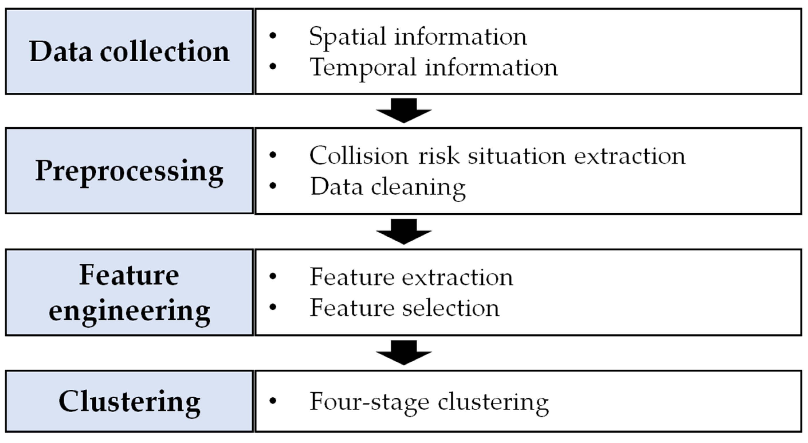
This section provides a data-driven approach as shown in Figure 1. The methodology includes data collection, preprocessing, feature engineering, and clustering steps. The authors collected ship traffic data (AIS) and geographic data (ENC). In the preprocessing step, obtained data were subsequently refined to extract CRSs. Features from the CRSs were designed, extracted, and selected in the feature engineering step. Then, in the clustering step, CRSs were categorized using multiple-stage clustering. Detailed steps are provided in the following subsections.

2.1. Data Collection

The collected data were AIS and ENC data. AIS data were provided by the Republic of Korea’s Ministry of Oceans and Fisheries. It consists of static, voyage-related, and dynamic information. ENC data comprises marine geographic information, such as land, buoys, and contours [33].

As shown in Figure 2, the area where various traffic situations between ships entering and departing was selected. The selected area, Incheon, Pyeongtaek, and Daesan ports, had an appropriate distribution of ENC data. Figure 2a shows the data points of AIS data, and Figure 2b indicates the aspects of geographic objects in the corresponding area.

The collection period of AIS data was one month, from 1 September 2019 to 30 September 2019. When considering the establishment of CRSs for the MASS test bed, the spatial and temporal size of the collected data is rather limited, but from the perspective of validation, the data size was appropriate.

2.2. Preprocessing

2.2.1. Collision Risk Situation Extraction

CRS extraction was conducted by recognizing ship-to-ship situations, finding geographic objects, and identifying CRSs that include traffic and geographic factors simultaneously. Each ship in the accumulated ship trajectories was selected as own ship (OS), and the target ships (TSs) within the designated distance to OS were recognized, as shown in Figure 3.

The criteria for recognizing ship-to-ship situation groups are defined in

Table 2. Ship-to-ship CRS extraction criteria.

Criteria	Object	Description
Ship’s length	OS	150 m~200 m
Ship’s SOG	OS	Over five knots
Distance	TS	Less than one nautical mile

. Overall, OSs were of a length (L.O.A) between 150 m and 200 m, and the speed was set to more than five knots to sort the sailing ships. Ships within one nautical mile from OS were recognized as TSs. In the distance calculation, the Euclidean distance was used. The length of the own ship can be considered rather limited, but it is selected according to the specification of the target ship of the funding project.

Afterward, the geographic objects were found among the ship-to-ship situations where geographic objects exist within one nautical mile from OSs. In selecting geographic objects, the authors focused on the physical obstacles, such as buoys, coastlines, bridges, depth contours, wrecks, pontoons, pylons, and bridge supports, as detailed in

Table 3. Physical objects from ENC data.

Categories	Abbreviations	Object Descriptions
Beacons	BCNCAR	Beacon, Cardinal
	BCNISD	Beacon, Isolated danger
Buoys	BOYISD	Buoy, Isolated danger
	BOYCAR	Buoy, Cardinal
	BOYLAT	Buoy, Lateral
	BOYSPP	Buoy, Special purpose
Depth	COALNE	Coastline
	LNDARE	Land area
	DEPCNT	Depth contour
	DEPARE	Depth area
	SOUNDG	Sounding
Obstacles	WRECKS	Wreck
	BRIDGE	Bridge
	OBSTRN	Obstruction
	PONTON	Pontoon
	PYLONS	Pylon/Bridge support

. Since the maximum draft of the extracted OS was 15m, the depth contours were restricted accordingly.

Consequently, 5906 cases of CRSs were extracted upon the contemplation of the above traffic and geographic factors. Figure 4 is the sample of extracted CRSs for one OS.

2.2.2. Data Cleaning

AIS data have errors. The timestamp intervals of all ships differed according to their SOG and communication status [34], and the heading has frequent errors, such as “zero” or “511” [35]. In order to handle errors, the time interval was regularized to one minute, and dynamic variables (COG, SOG, ship’s position) were interpolated by linear interpolation. The heading error was substituted for the COG [20] because the heading is an essential element in the determination of the encounter situation. Then, CRSs exceeding six-minute intervals were truncated.

2.3. Feature Engineering

2.3.1. Feature Extraction

CRSs were distinguished by three feature classes. One feature in the “Area class” classifies the spatial characteristics of CRSs. Another feature in “Own ship class” represents the traits of a ship’s navigating pattern. The other feature in the “Target ship” class distinguishes the relationship between OS and TS. Features extracted by the classes are shown in

Table 4. Extracted features.

Classes	Features	Descriptions
Area	Density of an ENC data point Number of lands Density of land datapoints Number of contours Density of contour datapoints	Number of all obstacle data points Number of land groups Number of land data points Number of contour lines Number of contour data points
Own ship	Standard deviation from COG Standard deviation from SOG	Course changing intensity Speed changing intensity
Target ship	Type of ship Type of encounter	Type of target ship Quadrant changes of the target ship

. Feature extraction used windowing. The window size was set to six minutes, and the moving size was set to three minutes.

In the area class, the features represent the degree of spatial constraint using the density of geographic objects in CRSs. DBSCAN is used to transform the adjacent objects’ data points into land and contour groups [36] to extract the “Number of lands” and “Number of contours.” The quantities of object data points in CRSs were extracted as “Density of ENC data points,” “Density of lands data points,” and “Density of contour data points.” The own ship class extracted the standard deviation of COG and SOG to represent the intensity of changes in course and speed, respectively [37]. In the target ship class, the authors re-categorized standard AIS types of ships into four types for effective clustering in

Table 5. Recategorization of ship type.

Type Code	Description	Recategorized
0	Not available (default)	N/A
1–19	Reserved for future use	N/A
20~29	Wing In the Ground (WIG)	Others
30	Fishing	Fishing (small)
31~32	Towing	Operation
33	Dredging or underwater operation	Operation
34	Diving operation	Operation
35	Military operation	Operation
36	Sailing	Fishing (small)
37	Pleasure craft	Fishing (small)
38~39	Reserved	N/A
40~49	High-speed craft (HSC)	Others
50	Pilot boat	Operation
51	Search and Rescue vessel	Operation
52	Tug	Operation
53	Port tender	Operation
54	Anti-pollution equipment	Operation
55	Las enforcement	Operation
56–57	Spare-Local vessel	Operation
58	Medical transport	Operation
59	Noncombatant ship (RR Resolution No.18)	Operation
60~69	Passenger ship	Commercial ship
70~79	Cargo ship	Commercial ship
80~89	Tanker ship	Commercial ship
90~99	Other types of ship	Others

.

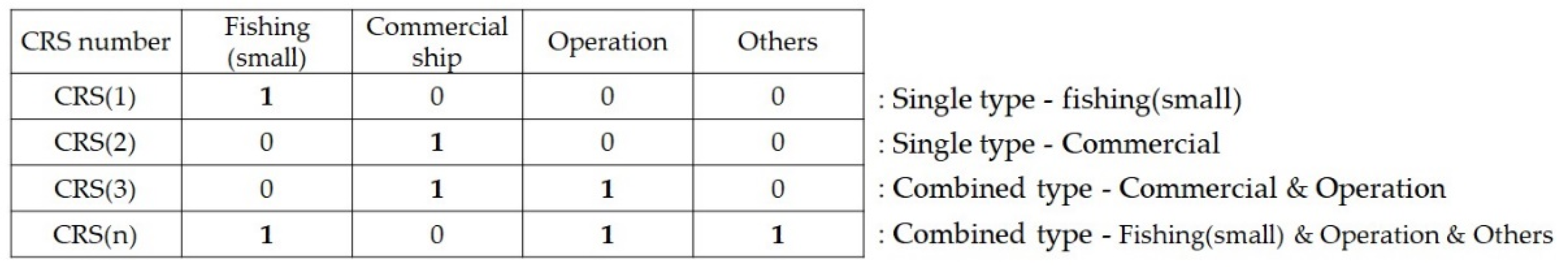
Afterward, newly defined types of ships were converted into a logical array. The logical array describes the composition of TS involved in each CRS. Figure 5 shows the example of the “type of ship” feature in the form of a logical array.

Similarly, “Type of encounter” was transformed into a logical array using the TS’s relative bearing changes. The relative bearing was converted into a Cartesian coordinate system. Then, the switches of relative position quadrants were calculated and described as a logical array [20]. Figure 6 show the example of the “Type of encounter” feature.

2.3.2. Feature Selection

The primary purpose of feature selection was to select the distinctive features for effective clustering. Since features in the “area” and “ownship” classes were continuous numerical values, the Laplacian rank method was an appropriate feature selection method [38]. The result of the Laplacian ranks of “area” and “ownship” features was derived distinctively, indicating the importance of the feature. On the contrary, features in the “target ship” class were independent enough to cluster; thus, all features in the “target ship” class were selected.

2.4. Clustering

Subsequently, the feature dataset of CRSs was classified through multiple-stage clustering. Multiple-stage clustering is an intuitive and interpretable method that keeps the accessibility of each cluster by providing results in stages [39].

2.4.1. First Stage Clustering

CRSs were classified according to the area’s spatial characteristics using the “area” class feature. The clustering algorithm used here was the K-means clustering algorithm. The distance measurement was the Euclidean distance, and an optimal number of clusters was selected using silhouette evaluation methods.

2.4.2. Second Stage Clustering

CRSs were distinguished according to the intensity of the own ship using the own ship class feature. The clustering algorithm adopted was the K-means clustering algorithm. The Euclidean distance was used for distance measurement. The optimal K of silhouette evaluation was employed in selecting cluster numbers required for applying the K-means algorithm.

2.4.3. Third Stage Clustering

This stage clustered CRSs using the feature “type of ship” in the TS class. The distance measurement was the hamming distance. Calculated pairwise distances between CRSs were applied to the linkage algorithm. The silhouette evaluation was used in the selection of an optimal number of clusters.

2.4.4. Fourth Stage Clustering

This stage grouped CRSs by the TS class’s feature “type of encounter.” The applied distance measurement was the hamming distance. The pairwise hamming distance between CRSs was applied to the linkage algorithm and clustered. The optimal K of the silhouette evaluation was employed in selecting cluster numbers required for using the K-means algorithm.

3. Result

3.1. Extraction and Selection of Features

The highest three features were selected in the “area” class, as shown in Figure 7a. One feature was selected in the “own ship” class feature, as described in Figure 7b.

Based on the feature selection result, the final adopted features are listed in

Table 6. List of selected features.

Class	Feature	Description
Area	The density of the ENC data point Number of lands The density of the contour datapoints	Number of data points of all geographic obstacles in the CRS Number of islands or lands in the CRS Number of contour data points in the CRS
Own ship	The standard deviation of COG	Represents how much the own ship changed course in the CRS
Target ship	Type of ship Type of encounter	Type of target ship (Static AIS data) in the CRS Quadrant change in target ship using relative bearing

. The features of the “area” class were comprised of “Density of ENC datapoint,” “Number of lands,” and “Density of Contours datapoints.” The selected feature of the OS class was the “Standard deviation of COG.” As for the “Target ship” class, the logical arrays describing the type of ship and type of encounter were the features selected.

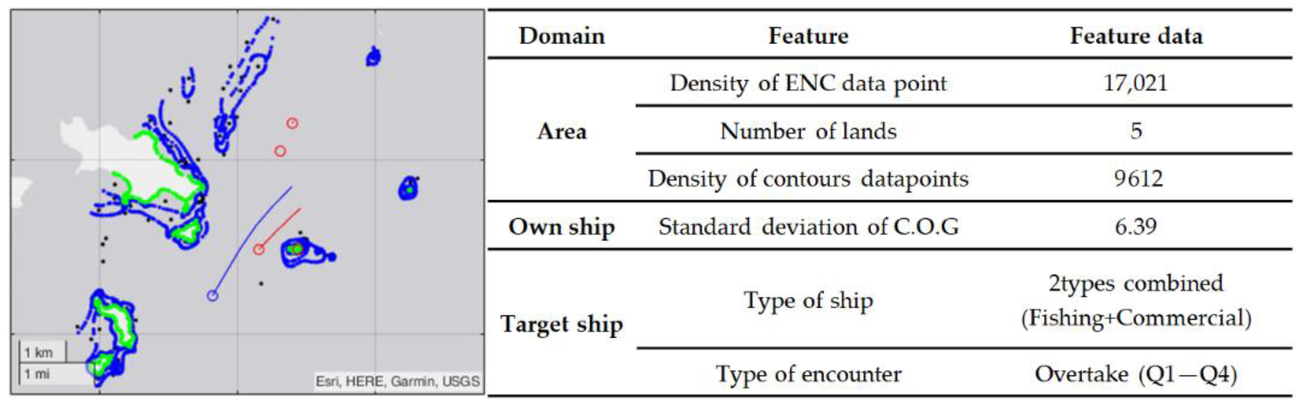
Figure 8 shows sample CRS and feature values. The figure on the left describes the CRS on the map. The green color indicates land, blue indicates depth contour, and the black dot indicates buoys. The initial position and direction of the OS are indicated using a blue circle and a line, and the red circle and line indicate TS. The figure on the right is the feature value that depicts the geometric navigation situation in numbers. The area used had 17,021 ENC data points and 5 land groups. Among the ENC data points, there are 9612 contour data points. The standard deviation of the OS course was 6.39, indicating a course change. Furthermore, the type of ship encountered was a combination of a fishing boat and a commercial ship, comprising an encounter-type situation where the OS overtook the TS on the starboard side.

3.2. Clustering Result

As a result of clustering, 5906 CRSs were categorized into 1393 groups. Figure 9 describes the division of each clustering stage. The first stage distinguished CRSs into three clusters based on the density of geographic objects. In the second stage, the three clusters from the first stage were subdivided into two groups by the OS maneuvering intensity. The third stage grouped the clusters by TS ship type. Finally, the last stage subdivided the clusters by the encounter type of TS. The results of each clustering are described in the subsection.

The lines at the final nodes (right end) are the clusters of similar collision risk situations. These lines were represented by grey lines and other colored lines based on the frequency. The colored lines indicate clusters containing multiple CRSs. These comprised 584 clusters, which explained 86.3% of the entire CRSs. The remaining grey lines are sole clusters, which occurred only once out of 5906 CRSs, and they were excluded from other clusters due to their complex and unique characteristics.

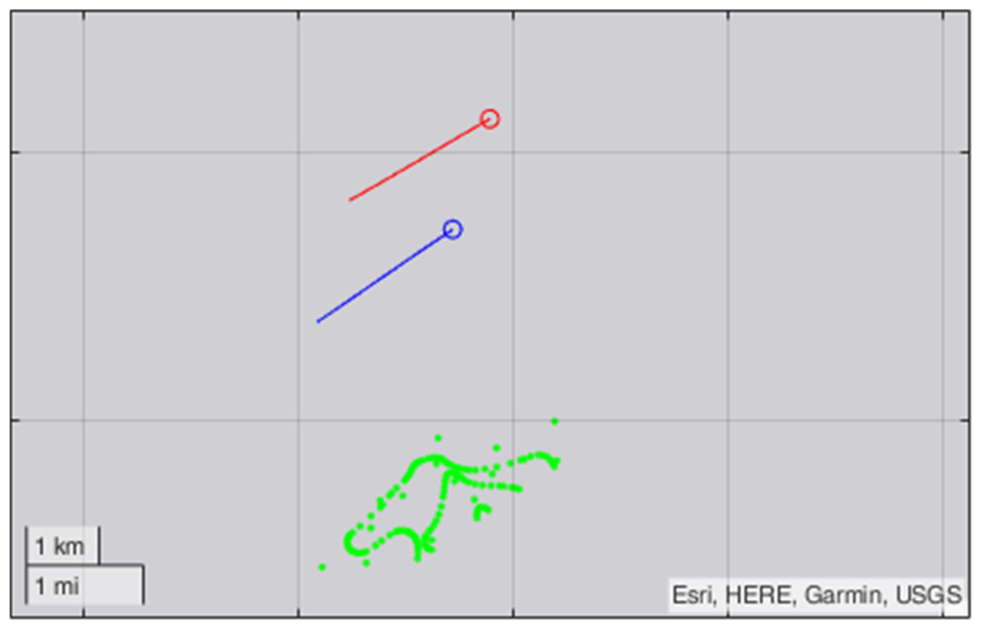
The red dotted line in Figure 9 is a sample CRS to explain the clustering result. As the line went through the clustering stages, CRSs were subdivided into detailed clusters. The navigation situation in Figure 10 is the corresponding sample CRS. Based on the criteria for each clustering stage, this CRS was interpreted as follows:

“The geographic condition of this CRS is less limited, and the movement of the own ship is stable. Therefore, the target ship is a commercial ship that follows the own ship from the starboard quarter.”

3.2.1. First Stage Clustering

This stage distinguished CRSs into three clusters based on the density of the geographic objects. As shown in Figure 11a, while the lowly restricted area was 62.9% of the total CRSs, the moderately restricted area was 29.8%, and the highly restricted area was 7.3%.

Figure 11b shows each cluster’s spatial distribution of the CRSs. While green indicates the geographic objects, the other three colors represented the clusters. Investigations revealed that the closer the area was to the port or inner land, the more it was classified as highly restricted. Contrastively, the farther the area, the more it was classified as lowly restricted.

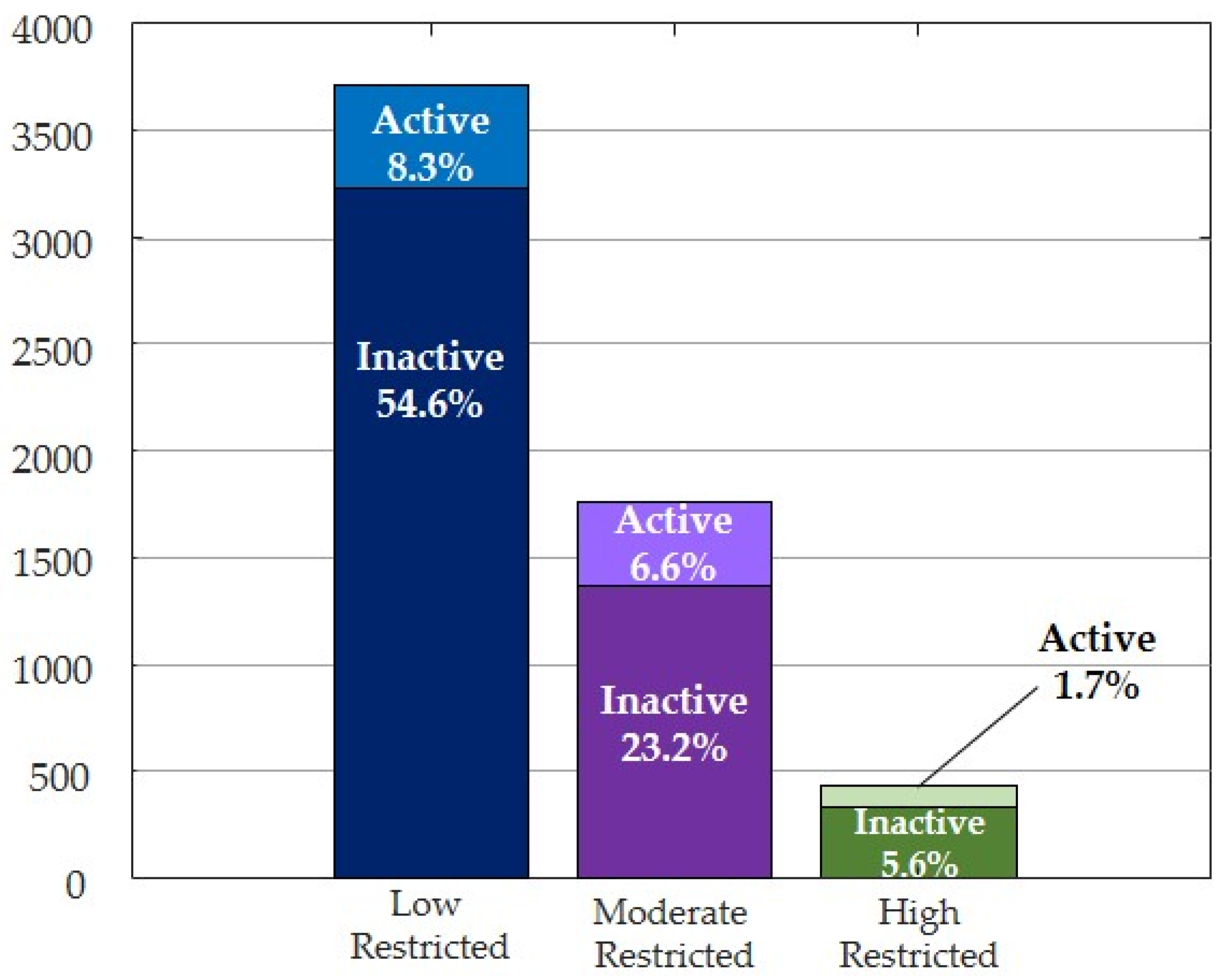
3.2.2. Second Stage Clustering

The own ship’s STD of COG was this clustering stage’s feature. This stage distinguished the CRSs into two groups, “Active” and “Inactive.” Figure 12 shows the ratio of the two intensity-based groups. Investigations revealed a difference in the inactive and active OS ratio by area. The ratio was 6.5:1 in the lowly restricted area, 3.5:1 in the moderately restricted area, and 3.29:1 in the highly restricted area. This indicates that the OS tended to move more actively in the highly restricted area than in the lowly restricted area.

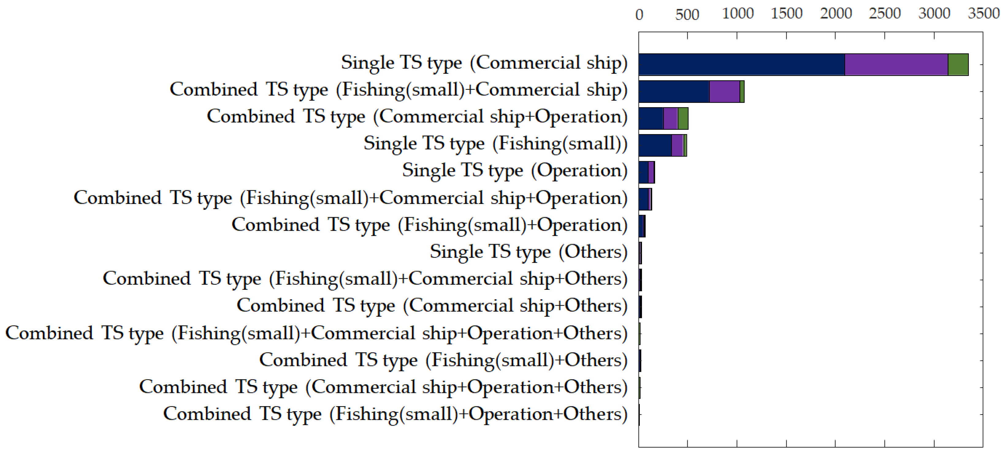
3.2.3. Third Stage Clustering

The result of clustering based on the type of TS differentiated the CTSs into 14 clusters. The type of TS not only includes the single type but also includes the combined TS types. As can be seen in Figure 13, the commercial ship is the main composition of the TS type. The highest three TS types include commercial ships. On the contrary, the others showed a low frequency, indicating that the more complex the combination of ship types, the lower the occurrence.

3.2.4. Fourth Stage Clustering

The final clustering stage identified 1393 CRS clusters based on the encounter type of TS. As mentioned in the clustering overview, CRS clusters can be labeled as multiple CRS groups and sole CRS groups. The multiple CRS group is the cluster with the plural CRSs, and the sole groups are clusters with one CRS excluded from any other clusters because the situation is complex and unique.

As shown in Figure 14a, while 574 multiple CRS groups contained 5097 CRSs, representing 86% of the total CRSs, the remaining 14% consisted of 809 sole CRS groups. Figure 14b shows the frequency of clusters highlighting the top 50 clusters of the ordinary group.

Accordingly, clusters could be separated into the “ordinary CRS” and “unique CRS” groups with particular characteristics. Figure 14c presents the characteristics of the “ordinary” and “unique” CRS groups by sample trajectory. In this figure, green represents the geographic obstacles, the blue circle and line indicate the position and direction of OS, and the red circle and line represent the position and direction of TS. Investigations revealed that the trait of the “Unique CRS” was based on the ship’s type and encounter type complexity. In particular, the high complexity of the ship’s type and encounter type was a dominant factor in the lowly restricted area. Nevertheless, since the environment had a low occurrence, a unique situation could be classified with only a small number of TS in the highly restricted environment.

4. Discussion

This study’s methodology presents a data-driven approach to extracting and categorizing CRSs to develop a systematic method for designing test beds for an objective evaluation of the collision avoidance system of MASSs.

Navigational features of three classes were generated and adopted to multiple-stage clustering, then 5097 CRSs were categorized into 1393 clusters. The clustering results showed the following achievements of this methodology:

First, the area class clustering classified CRSs as lowly restricted, moderately restricted, and highly restricted, along with ratios. Notably, the ratio was highest in the “lowly restricted” and lowered as it approached the port or inland. It implies that the collision risk situation of MASS will occur more in lowly restricted water than near ports. Therefore, this result presented a basis for the area selection of the MASS test. Second, the cluster by the type of target ship presented a composition of the target ship types with ratios. This result is expected to be used in generating target ships in collision avoidance tests of MASSs. The authors expect that collision avoidance tests with various combinations of target ships will improve the reliability of the MASS collision avoidance algorithm. Third, the encounter type was classified into ordinary and unique groups according to frequency. The ordinary group comprised CRSs in which the same situations had occurred more than once in the entire period. The unique group comprises the CRSs excluded from any cluster because the situation was very complicated. These findings suggest two factors to be considered when constructing a test bed: one is the objective basis for the composition of basic navigation scenarios, and the other is the ground for establishing harsh scenarios for debugging collision avoidance algorithms.

5. Conclusions

This study presented a methodology for developing an objective and realistic collision risk situation to test the collision avoidance algorithm for MASS. It differs from previous studies because the collision risk situation was extracted as data-driven, considering the geographic environment.

Collision risk situations were extracted where traffic and geographic factors coexist within one nautical mile from the own ship. Afterward, these situations were categorized through four-stage clustering.

Consequently, the results presented classified collision risk situations from sea area, type of target ship, and type of encounter situations. Occurrence rates of CRSs were also provided on the sea area and target ship type. These results are expected to apply to the design of the collision avoidance test.

In addition, ordinary and unique CRSs were identified. Identifying a unique collision risk situation was the most significant achievement of this methodology. Although these unique situations were complex and infrequent navigations, they were likely encountered during MASS sailing during its lifetime. Therefore, applying this unique case to the test bed should complement and improve MASS’s collision avoidance system.

However, despite our achievements, limitations to this study also exist. The limitations identified through the application of this methodology are the limitations of ship and port selection, feature engineering, and clustering. Therefore, these limitations will be improved in future works.

First, geographic and ship traffic characteristics were different for each sea area. Hence, future research on various sea areas and ports should develop a generalized collision risk situation scenario.

Second, since the own ship designated with a specific size needed to be applied based on ship type and various sizes, the size of other ships should also be identified as a future consideration.

Third, the situation classification using the quadrant change of the Cartesian coordinate system presented in this study still has an ambiguous distinction between head-on and overtaking situations. In future studies, it is necessary to improve these shortcomings using the ship’s speed, course, or duration of the situation.

Lastly, while a feature composed of three classes needs to be established from various perspectives, improvements in the design of clustering methods and multiple stages are required.

References

- Felski, A.; Zwolak, K. The ocean-going autonomous ship—Challenges and threats. J. Mar. Sci. Eng. 2020, 8, 41. [Google Scholar] [CrossRef]
- Kretschmann, L.; Burmeister, H.; Jahn, C. Analyzing the economic benefit of unmanned autonomous ships: An exploratory cost-comparison between an autonomous and a conventional bulk carrier. Res. Transp. Bus. Manag. 2017, 25, 76–86. [Google Scholar] [CrossRef]
- Ait Allal, A.; Mansouri, K.; Youssfi, M.; Qbadou, M. Toward a study of environmental and social impact of autonomous ship. In Euro-Mediterranean Conference for Environmental Integration; Springer: Berlin/Heidelberg, Germany, 2017; pp. 1709–1711. [Google Scholar]
- Jalonen, R.; Tuominen, R.; Wahlström, M. Safety of Unmanned Ships-Safe Shipping with Autonomous and Remote Controlled Ships; Aalto University: Espoo, Finland, 2017. [Google Scholar]
- Rokseth, B.; Haugen, O.I.; Utne, I.B. Safety verification for autonomous ships. In MATEC Web of Conferences; EDP Sciences: Les Ulis, France, 2019; p. 02002. [Google Scholar]
- European Maritime Safety Agency. Annual Overview of Marine Casualties and Incidents. 2021. Available online: https://www.emsa.europa.eu/newsroom/latest-news/download/6955/4266/23.html (accessed on 23 August 2022).
- Ringbom, H. Regulating autonomous ships—Concepts, challenges and precedents. Ocean Dev. Int. Law 2019, 50, 141–169. [Google Scholar] [CrossRef]
- Ceyhun, G.C. The impact of shipping accidents on marine environment: A study of Turkish seas. Eur. Sci. J. 2014, 10, 10–23. [Google Scholar]
- Porres, I.; Azimi, S.; Lilius, J. Scenario-based testing of a ship collision avoidance system. In Proceedings of the 2020 46th Euromicro Conference on Software Engineering and Advanced Applications (SEAA), Portoroz, Slovenia, 26–28 August 2020; pp. 545–552. [Google Scholar]
- Pedersen, T.A.; Glomsrud, J.A.; Ruud, E.; Simonsen, A.; Sandrib, J.; Eriksen, B.H. Towards simulation-based verification of autonomous navigation systems. Saf. Sci. 2020, 129, 104799. [Google Scholar] [CrossRef]
- Shokri-Manninen, F.; Vain, J.; Waldén, M. Formal verification of colreg-based navigation of maritime autonomous systems. In International Conference on Software Engineering and Formal Methods; Springer: Berlin/Heidelberg, Germany, 2020; pp. 41–59. [Google Scholar]
- Kufoalor, D.K.M.; Johansen, T.A.; Brekke, E.F.; Hepsø, A.; Trnka, K. Autonomous maritime collision avoidance: Field verification of autonomous surface vehicle behavior in challenging scenarios. J. Field Robot. 2020, 37, 387–403. [Google Scholar] [CrossRef]
- Porres, I.; Azimi, S.; Lafond, S.; Lilius, J.; Salokannel, J.; Salokorpi, M. On the verification and validation of ai navigation algorithms. In Proceedings of the Global Oceans 2020: Singapore–US Gulf Coast, Biloxi, MS, USA, 5–30 October 2020; pp. 1–8. [Google Scholar]
- Shaobo, W.; Yingjun, Z.; Lianbo, L. A collision avoidance decision-making system for autonomous ship based on modified velocity obstacle method. Ocean Eng. 2020, 215, 107910. [Google Scholar] [CrossRef]
- Cho, Y.; Han, J.; Kim, J. Efficient COLREG-compliant collision avoidance in multi-ship encounter situations. IEEE Trans. Intell. Transp. Syst. 2020, 23, 1899–1911. [Google Scholar] [CrossRef]
- Han, J.; Cho, Y.; Kim, J.; Kim, J.; Son, N.; Kim, S.Y. Autonomous collision detection and avoidance for ARAGON USV: Development and field tests. J. Field Robot. 2020, 37, 987–1002. [Google Scholar] [CrossRef]
- Guo, S.; Zhang, X.; Zheng, Y.; Du, Y. An autonomous path planning model for unmanned ships based on deep reinforcement learning. Sensors 2020, 20, 426. [Google Scholar] [CrossRef]
- Bakdi, A.; Glad, I.K.; Vanem, E. Testbed scenario design exploiting traffic big data for autonomous ship trials under multiple conflicts with collision/grounding risks and spatio-temporal dependencies. IEEE Trans. Intell. Transp. Syst. 2021, 22, 7914–7930. [Google Scholar] [CrossRef]
- Fiskin, R.; Atik, O.; Kisi, H.; Nasibov, E.; Johansen, T.A. Fuzzy domain and meta-heuristic algorithm-based collision avoidance control for ships: Experimental validation in virtual and real environment. Ocean Eng. 2021, 220, 108502. [Google Scholar] [CrossRef]
- Hwang, T.; Youn, I. Navigation Situation Clustering Model of Human-Operated Ships for Maritime Autonomous Surface Ship Collision Avoidance Tests. J. Mar. Sci. Eng. 2021, 9, 1458. [Google Scholar] [CrossRef]
- Chun, D.; Roh, M.; Lee, H.; Ha, J.; Yu, D. Deep reinforcement learning-based collision avoidance for an autonomous ship. Ocean Eng. 2021, 234, 109216. [Google Scholar] [CrossRef]
- Wu, X.; Liu, K.; Zhang, J.; Yuan, Z.; Liu, J.; Yu, Q. An Optimized Collision Avoidance Decision-Making System for Autonomous Ships under Human-Machine Cooperation Situations. J. Adv. Transp. 2021, 2021, 7537825. [Google Scholar] [CrossRef]
- Zhang, X.; Wang, C.; Jiang, L.; An, L.; Yang, R. Collision-avoidance navigation systems for Maritime Autonomous Surface Ships: A state of the art survey. Ocean Eng. 2021, 235, 109380. [Google Scholar] [CrossRef]
- Sawada, R.; Sato, K.; Majima, T. Automatic ship collision avoidance using deep reinforcement learning with LSTM in continuous action spaces. J. Mar. Sci. Technol. 2021, 26, 509–524. [Google Scholar] [CrossRef]
- Zhang, L.; Mou, J.; Chen, P.; Li, M. Path planning for autonomous ships: A hybrid approach based on improved apf and modified vo methods. J. Mar. Sci. Eng. 2021, 9, 761. [Google Scholar] [CrossRef]
- Torben, T.R.; Glomsrud, J.A.; Pedersen, T.A.; Utne, I.B.; Sørensen, A.J. Automatic simulation-based testing of autonomous ships using Gaussian processes and temporal logic. Proc. Inst. Mech. Eng. Part O J. Risk Reliab. 2022. [Google Scholar] [CrossRef]
- Akdag, M.; Fossen, T.I.; Johansen, T.A. Collaborative Collision Avoidance for Autonomous Ships Using Informed Scenario-Based Model Predictive Control. In Proceedings of the 14th IFAC Conference on Control Applications in Marine Systems, Robotics, and Vehicles, Lyngby, Denmark, 14 March 2022. [Google Scholar]
- Li, M.; Mou, J.; He, Y.; Zhang, X.; Xie, Q.; Chen, P. Dynamic trajectory planning for unmanned ship under multi-object environment. J. Mar. Sci. Technol. 2022, 27, 173–185. [Google Scholar] [CrossRef]
- Xing, S.; Xie, H.; Zhang, W. A method for unmanned vessel autonomous collision avoidance based on model predictive control. Syst. Sci. Control Eng. 2022, 10, 255–263. [Google Scholar] [CrossRef]
- Hagen, I.B.; Kufoalor, D.; Johansen, T.A.; Brekke, E.F. Scenario-Based Model Predictive Control with Several Steps for COLREGS Compliant Ship Collision Avoidance. Available online: https://folk.ntnu.no/torarnj/Comparison.pdf (accessed on 8 September 2022).
- Yu, Y.; Chen, L.; Shu, Y.; Zhu, W. Evaluation model and management strategy for reducing pollution caused by ship collision in coastal waters. Ocean Coast Manag. 2021, 203, 105446. [Google Scholar] [CrossRef]
- Teixeira, A.P.; Guedes Soares, C. Risk of maritime traffic in coastal waters. In Proceedings of the International Conference on Offshore Mechanics and Arctic Engineering, Madrid, Spain, 17–22 June 2018; American Society of Mechanical Engineers: New York, NY, USA, 2018; p. V11AT12A025. [Google Scholar]
- Robards, M.D.; Silber, G.K.; Adams, J.D.; Arroyo, J.; Lorenzini, D.; Schwehr, K.; Amos, J. Conservation science and policy applications of the marine vessel Automatic Identification System (AIS)—A review. Bull Mar. Sci. 2016, 92, 75–103. [Google Scholar] [CrossRef]
- Guo, S.; Mou, J.; Chen, L.; Chen, P. An Anomaly Detection Method for AIS Trajectory Based on Kinematic Interpolation. J. Mar. Sci. Eng. 2021, 9, 609. [Google Scholar] [CrossRef]
- IMO. Available online: https://wwwcdn.imo.org/localresources/en/OurWork/Safety/Documents/AIS/Resolution%20A.1106(29).pdf (accessed on 23 August 2022).
- Liu, B.; de Souza, E.N.; Matwin, S.; Sydow, M. Knowledge-based clustering of ship trajectories using density-based approach. In Proceedings of the 2014 IEEE International Conference on Big Data (Big Data), Washington, DC, USA, 27–30 October 2014; pp. 603–608. [Google Scholar]
- Zhou, Y.; Daamen, W.; Vellinga, T.; Hoogendoorn, S.P. Ship classification based on ship behavior clustering from AIS data. Ocean Eng. 2019, 175, 176–187. [Google Scholar] [CrossRef]
- He, X.; Cai, D.; Niyogi, P. Laplacian score for feature selection. In Advances in Neural Information Processing Systems; MIT Press: Cambridge, MA, USA, 2005; Volume 18. [Google Scholar]
- Scheiner, N.; Appenrodt, N.; Dickmann, J.; Sick, B. A multi-stage clustering framework for automotive radar data. In Proceedings of the 2019 IEEE Intelligent Transportation Systems Conference (ITSC), Auckland, New Zealand, 27–30 October 2019; pp. 2060–2067. [Google Scholar]
Figure 1.
Workflow of the proposed methodology.
Figure 2.
Spatial information obtained from the AIS and ENC data: (a) AIS data points in the selected area, (b) Distribution os ENC data points in the selected area.
Figure 3.
Ship-to-ship situation recognized from the AIS data.
Figure 4.
CRSs including traffic and geographic factors.
Figure 5.
Schematic showing the feature extraction process of a “type of ship” array.
Figure 6.
Schematic showing the feature extraction process of a “type of encounter” array. The sample situation was converted into relative bearing and distance in the Cartesian coordinate system. The quadrant changes were calculated and converted as a logical array(red box).
Figure 7.
Results from the feature selection of the area and OS classes. (a) Area class. (b) OS class.
Figure 8.
Features in sample CRS.
Figure 9.
Topology of the clustering results.
Figure 10.
Visualization of the sample CRS. The green color indicates the ENC object, the blue indicates the own ship, and the red indicates the target ship.
Figure 11.
Ratio and trajectory distribution of the first stage clustering result: (a) The ratio of each area, (b) the Spatial distribution of each cluster.
Figure 12.
The ratio of clusters in the second stage cluster.
Figure 13.
Frequency of each type of ship combination.
Figure 14.
Ratio and sample trajectories of the ordinary and unique CRSs: (a) Ratio of “Ordinary”, and “Unique” group, (b) The frequency of clusters in the ordinary group, (c) Sample trajectory of Ordinary and Unique group.