Article

Consequence Analysis of Accidental LNG Release on the Collided Structure of 500 cbm LNG Bunkering Ship

1
Department of Marine Design Convergence Engineering, Pukyong National University, Busan 48513, Korea
2
Department of Naval Architecture and Marine System Engineering, Pukyong National University, Busan 48513, Korea
3
Department of Offshore Platform Research Division, Korea Research Institute of Ships and Ocean Engineering, Daejeon 34103, Korea
*
Author to whom correspondence should be addressed.
J. Mar. Sci. Eng. 2022, 10(10), 1378; https://doi.org/10.3390/jmse10101378
Submission received: 12 August 2022 / Revised: 12 September 2022 / Accepted: 21 September 2022 / Published: 26 September 2022
(This article belongs to the Special Issue Ship Collision Risk Assessment)

Abstract

:
The growing demand for liquefied natural gas (LNG)-fueled ships necessitates the establishment of an LNG bunkering facility. Ship-to-ship (STS) is one of the most practical forms of LNG bunkering systems. Although there are benefits to the LNG bunkering of ships, risk and safety issues are a concern due to the volatile cargo. Ship collision could result in accidental LNG release. The purpose of this study was to build LNG leakage scenarios, establish critical zones based on gas concentrations, and estimate the temperature reduction in a bunkering ship’s structure resulting from the use of cryogenic fluid. The condition of a target ship’s structure, both intact and when damaged due to collision, was considered. Leak size, leak direction, leak position, release rate, and reservoir pressure were included as leak parameters, and environmental parameters, such as the wind direction, wind speed, and ambient temperature, were also included. The release duration was set based on the shutdown duration of the emergency shutdown valve (ESD). A total of 72 leakage scenarios were generated for the main CFD analysis. Convergence tests were conducted to determine the appropriate grid and iteration numbers for a computational fluid dynamics (CFD) simulation. The gas dispersion characteristics and the cryogenic flow impact on the LNG bunkering ship’s structure are discussed through a parametric study.

1. Introduction

Since 2010, the International Convention for the Prevention of Pollution from Ships (MARPOL) Protocol Annex VI has been enforced to minimize sulfur oxide (SOX), nitrogen oxide (NOX), and particulate matter emissions [1]. Emission control areas (ECA) have been established in several regions that prohibit ships from producing excess pollutants. According to Annex VI Regulations 13 and 14, ships must reduce SOX and NOX emissions to 0.10% m/m and 3.4 g/kWh, respectively, inside the ECA [1]. To conform to these regulations, liquefied natural gas (LNG) can be utilized as an alternative fuel for ships. As a result, there is significant demand for LNG-fueled ships—116 vessels have been in service since 2018, with 120 more under construction or with confirmed orders [2]. Consequently, it is predicted that LNG consumption will increase from 1.27 to 3.01 million tonnes per annum for the shipping industry alone [3]. This would require a new LNG bunkering facility in each port. There are several LNG bunkering methods, including truck-to-ship (TTS), pipeline-to-ship (PTS), and ship-to-ship (STS). These methods are applicable depending on operating conditions, port topography, and the allowable vessel size in the port [4,5]. TTS is unlikely to be suitable to meet the significant demands for LNG bunkering in the future. However, its benefits include high accessibility, easy operation, and low initial investment, and it remains a popular method [6]. PTS and STS methods are more feasible for increasing LNG storage capacity. In addition to its suitability for addressing the LNG capacity issue, STS can overcome topographic disadvantages and is suitable for ships with short port turnaround times [7]. Since STS requires a bunkering vessel unit, past research has been concerned with the design of the LNG storage tank. The common shape of the LNG storage tank is the IMO Type-C independent tank, which can sustain the pressure increases up to the maximum design pressure without affecting the gas-fuel supply and it does not need a boil-off gas treatment [8]. However, the volume efficiency is lower than other types of non-pressurized LNG storage tanks [8]. Past research presented a study to optimize the LNG storage tank shape by adopting the Lattice pressure vessel which can increase the volume efficiency [9]. Another improvement in the LNG bunkering research is the study of the characteristics and control of the heading angle of the floating LNG bunkering terminal. The optimum heading angle along ships during the bunkering process can improve the loading and off-loading performance. It can reduce the relative motions of the moored vessels [10].
In regards to the research on risk modeling, the SAFEDOR risk model identifies generic types of accident affecting LNG carriers, which are collision, grounding, contact, fire/explosion, and accidents during loading/unloading [11]. These accident types contribute most to risk according to their probability and severity based on data from the 1964 to 2005 accident database. These categories of accident can happen on all types of ship. The possibility of accident escalation is significant for LNG carriers due to the volatility of the cargo [11]. For example, a collision accident on an LNG carrier that causes damage to the cargo hold or LNG line could lead to LNG leakage.
Storage/distribution facilities and loading/unloading activities are associated with frequent accidental gas releases which are related to the LNG bunkering of ships, according to the electronic major accident report system (eMARS) database [12]. Unignited LNG release creates significant risks, such as asphyxiation, cold vapor inhalation, and cryogenic burns to personnel [6,13]. When the released gas accumulates and is ignited, it can lead to deflagration or detonation, which could endanger objects surrounding the LNG bunkering ship [6,14].
Computational fluid dynamics (CFD) simulation can assist in the evaluation of safety and loss prevention in the design of LNG bunkering ships. CFD is a reliable method that can simulate complex gas dispersion, jet or pool fires, and vapor cloud explosion (VCE). Several studies have been undertaken utilizing these kinds of CFD models for ships or offshore structures [15,16,17,18,19,20]. Tools such as Kameleon Fire Ex (KFX) incorporate both gas boiling and spreading problems, a turbulence model, interactions with obstructions, and heat transfer problems to simulate unignited gas release [21,22,23].
CFD simulation can also be useful for predicting the boundary of hazardous or critical zones. This zone is designated using a three-dimensional geometry to represent the occurrence of flammable gas in the event of an accidental release [7,18,24]. Several studies have used the critical zone as a primary outcome that is determined by measuring the concentration of released gas above its lower flammability limit (LFL) [6,25,26,27,28,29]. The purpose of the critical zone is to eliminate ignition sources around the bunkering installation, and to restrict access to it so that only essential personnel and activities are allowed in this zone [7,29,30]. This can help to prevent personnel injuries or fatalities, as well as the possibility of VCE, by minimizing ignition sources in the zone.
Further types of risk analysis, such as advanced cryogenic risk analysis (ACRA), is suggested for cases of temperature reduction due to cryogenic release in any offshore or onshore unit [31]. This method includes assessment of the presence of structures, equipment, barriers, and wind conditions for incorporation into a CFD simulation. It also involves heat transfer calculation to estimate the ductile to brittle transition temperature (DTBTT) of the exposed structure [13,31]. Such embrittlement can weaken the structural steel and escalate to a structural collapse, particularly if an accidental load strikes the ship [13,32]. Therefore, the temperature profile obtained in a CFD simulation can be utilized for advanced cryogenic spill protection optimization (ACSPO) for a load. The ACSPO approach involves thermal–structural analysis that is simulated using the finite element (FE) method. It is useful to estimate the load capacity of a structure in the event of cryogenic exposure [31]. Table 1 presents past studies that have involved temperature reduction analyses of structures.
The purpose of the present study was to develop LNG release scenarios that take into account leak and environmental parameters, as well as to provide an analysis of temperature reduction in the structure of LNG bunkering ships in the event of an accidental LNG release, and to determine critical zones based on the flammability of released gas. Figure 1 presents a framework for the study that highlights two important steps in the temperature reduction analysis.
I. Accidental Release Scenario: Details of the bunkering system were provided for an LNG bunkering ship. Damaged parts of the ship geometry owing to a collision, and the ship geometry comprising both intact and damaged elements, were represented. The CFD analysis considered variables such as leak size, mass flow rate, reservoir pressure, leak position, and leak duration. Wind speed, wind direction, and ambient temperature were also considered. The thermal properties of LNG and steel, such as density, thermal conductivity, and specific heat, were considered in the KFX material settings. A total of 72 scenarios were then selected for CFD analysis.
II. CFD Simulation: All LNG release scenarios were simulated in KFX. To obtain a suitable grid number and time interval for the LNG release model, a grid convergence test (GCT) and iteration convergence test (ICT) were conducted. The result of gas cloud volume analysis was then used to investigate gas accumulation and dispersion. At the LNG flammability limits, which represent the gas contour, the critical zone was also determined. Finally, to predict damaged components as a result of cryogenic effect, the temperature profile in the LNG bunkering structure was obtained.

2. Determination of Leakage Scenario

The leakage scenario determination was based on parameters suggested in ACRA, i.e., the ship structure as obstructions, weather parameters, and generic release frequencies. In this section, the procedure of leakage scenario determination is presented.

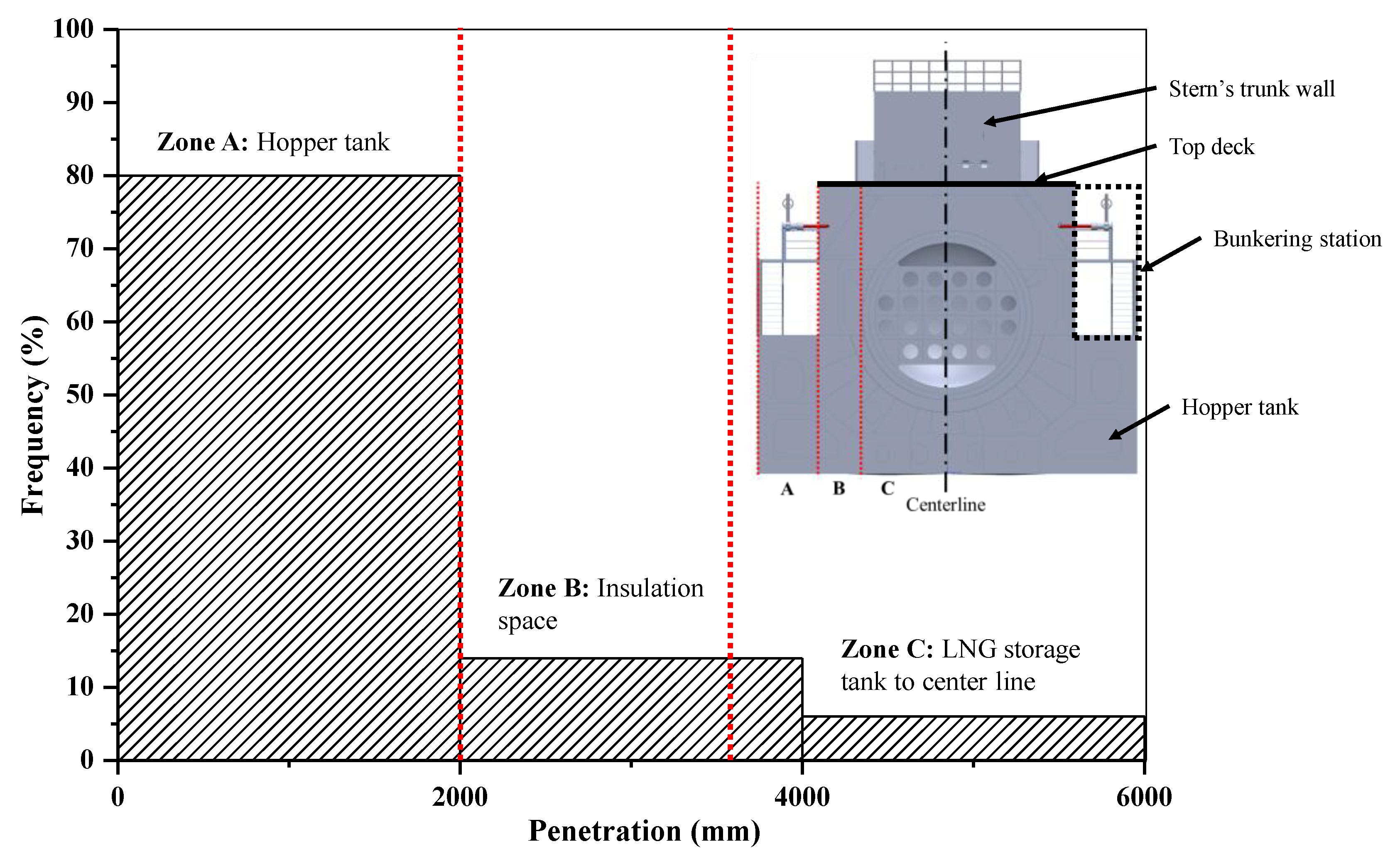
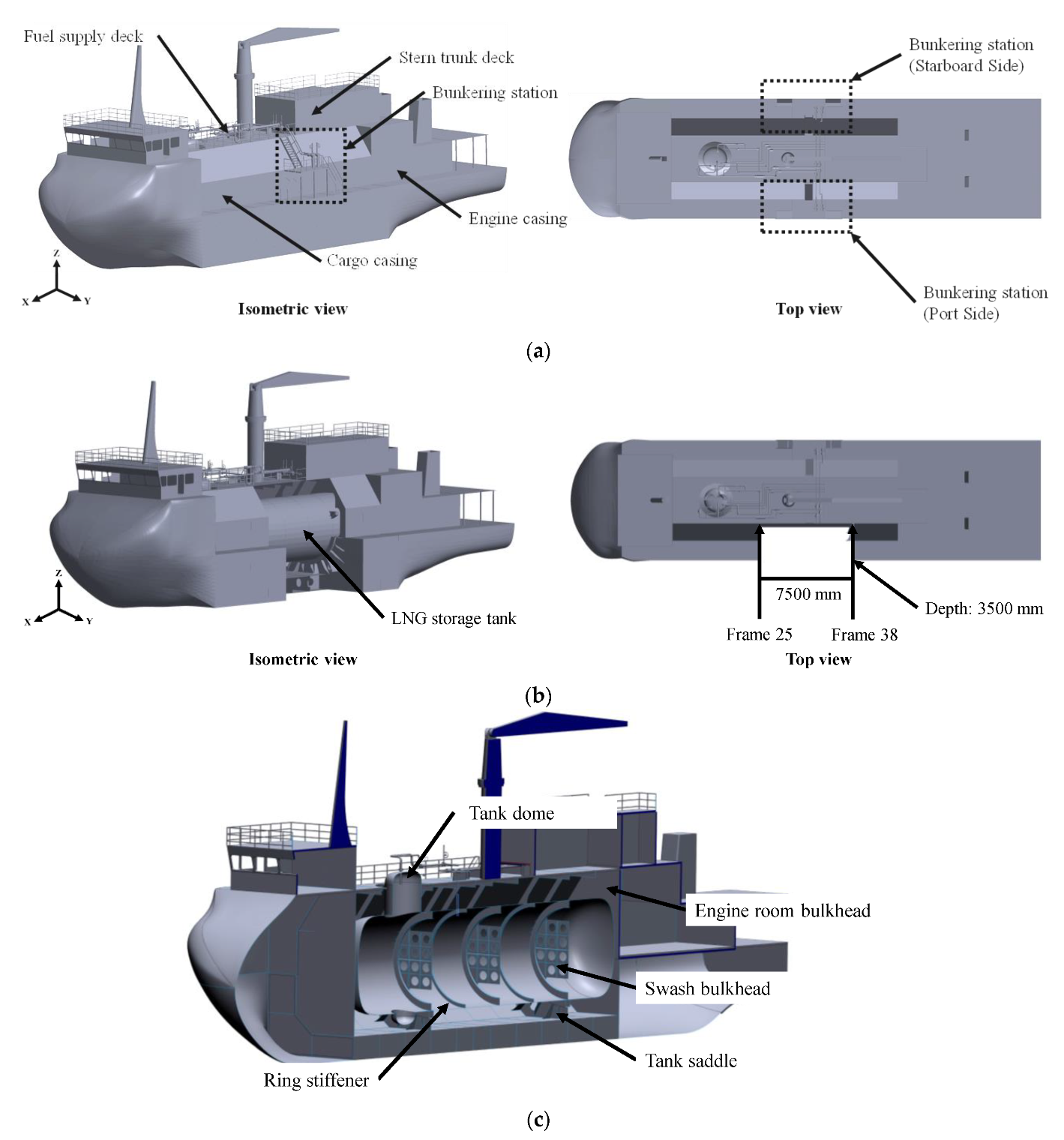
2.1. Intact and Damaged Geometries of the Ship

An LNG bunkering ship was used for gas dispersion simulation as a target ship; the ship’s dimensions are given in Table 2. This study assumed two different causes of an accidental release event that can affect ship geometry conditions. An intact ship was used for the analysis in which equipment failure causes LNG release. Equipment failure means damage to, or malfunction of, apparatus that initiates LNG release—for example, the fracture of a pipe or its flange joint due to the poor quality of material or maintenance error [36]. In several studies, LNG release initiated by a crack due to fatigue, wear and tear, or breach due to dropped objects penetrating equipment, was investigated [16,18,37]. Another potential cause of LNG release is ship collision that damages LNG bunkering system equipment [16]. Here, the energy associated with the effect of striking indirectly damages equipment. The collision energy can distort the flange joint between pipe-pipe and pipe-valve connections and initiate LNG release.
Previously obtained collision analysis data were used to define the damage region for CFD modeling [38]. The LNG bunkering ship was struck by the bow of the striking ship. In this case, the wrecked part was located on the port side, or the side that was facing the sea from the LNG bunkering ship, during the bunkering process [38]. Factors such as displacement, speed, and strike angle of the striking ship can result in different depth penetration of the struck ship [38]. The damage region was selected by considering the mid-level penetration frequencies and severity to determine the likelihood and significance of consequences. Figure 2 shows several zones that illustrate the depth penetration and its frequency. Zone A refers to penetration from the ship’s side shell to the insulation space or hopper tank region. The entire insulation space is located in Zone B, and Zone C includes the LNG storage tank to the ship’s centerline.
The penetration region was categorized into zones A, B, and C, which represent slight, middle, and severe penetrations, respectively. Zone B, which has 3500 mm depth penetration, was selected to represent the damaged condition. The degraded region was located at frames 25 to 38 which have a width of 7500 mm, since the target ship was struck around the midship on the portside. With these assumptions and considerations, the damaged ship can be modeled. Figure 3 shows both models of the LNG bunkering ship. The LNG bunkering ship was built with two bunkering stations located on each side of the ship so that it can simultaneously serve two ships. Figure 3b shows that the bunkering station does not exist on the port side of the damaged model. In addition, there is an opening in the cargo casing that exposes the LNG storage tank. The engine room is, however, secure since there is a bulkhead that separates the cargo hold and engine room, as shown in Figure 3c. The current LNG bunkering ship stores the LNG cargo inside a Type-C independent tank. Two tank saddles are installed below the storage tank to secure it inside the cargo casing. The Type-C tank was built with three swash bulkheads to decrease the sloshing effect. In addition, two ring stiffeners were installed to ensure adequate strength of the storage tank. The tank dome emerges onto the top deck or fuel supply deck where several valves were installed.

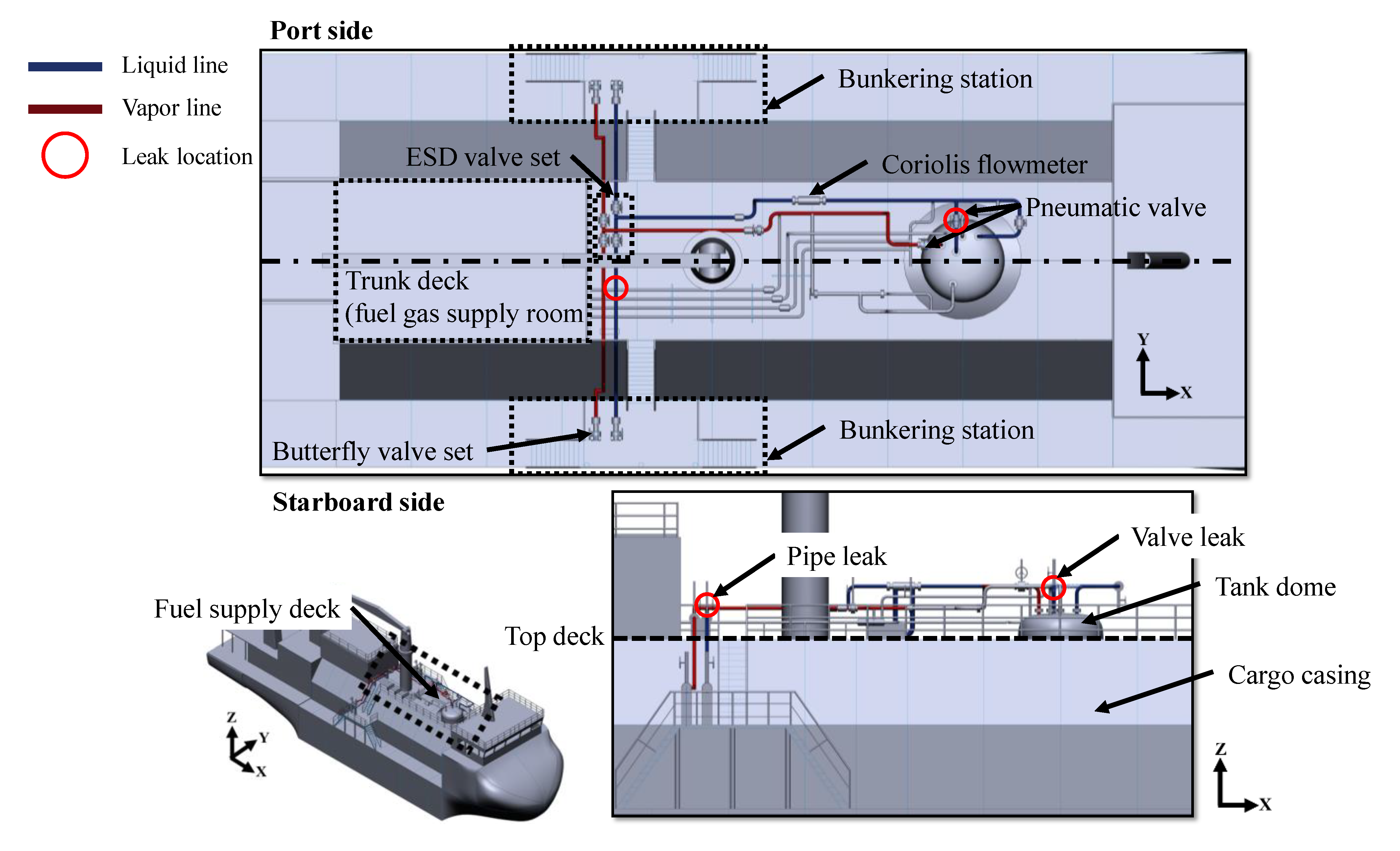
2.2. Leakage Parameter

To ensure the credibility of data for the leakage scenario, a generic release frequency assessment was undertaken to provide information on the frequency relative to the leak diameter for various items of LNG bunkering equipment. A number of institutions and associations have issued data directories of LNG release likelihood, including the International Association of Oil and Gas Producers (OGP) and the UK Health and Safety Executive (UK HSE) [39]. In this study, the OGP publication, “Risk Assessment Data Directory-Process Release Frequencies” was used to define the leak diameters for a valve and a pipe [40].
The LNG bunkering system is operated using 100.50 mm pipe for its nominal diameter installed on the LNG filling pipeline. The LNG cargo is loaded and unloaded via this pipeline. For the nominal diameter of the LNG filling line, a six-inch or 150 mm tabulation of leak frequency was used as recommended by the OGP directory. The hole diameters from the OGP tabulation were 3.0, 10.0, and 50.0 mm, representing minor, medium, and major severity, respectively. To avoid insignificant results, extreme minor severity, and extreme major severity with a hole diameter range larger than 150 mm were not used. The CFD simulation requires a release direction to the ship’s stern for all leak positions and the mass flow rate (kg/s) parameter. The mass-flow rate problem can be addressed using an equation for the choked-flow condition, which can be expressed as follows [41],
m ˙ = ρ υ A = p 0 ρ 0 γ 1 2 2 γ + 1 γ + 1 2 γ 1 π d 2 4
where is the mass flow rate (kg/s); ρ is the fluid density (kg/m3), which is 427.58 kg/m3 at −163.00 °C for LNG [42]; υ is the fluid velocity (m/s); p0 is the initial pressure (Pa), which is 5.00 bar at the LNG bunkering line; γ is the heat capacity ratio, which is 2.31 for LNG [41]; and d is the hole diameter (m). Table 3 shows the leak frequency tabulation including the hole diameters and mass flow rates that were used in the study. The leak was sourced from the pneumatic valve and a pipe, as shown in Figure 4. To simplify the scenarios, the same leak location was applied to both intact and damaged models. Furthermore, the leak was stopped 15 s after initial gas release. This assumption was based on the shutdown duration of the emergency shutdown valve installed on the gas supply system. This release duration was also used as the simulation time input in KFX.

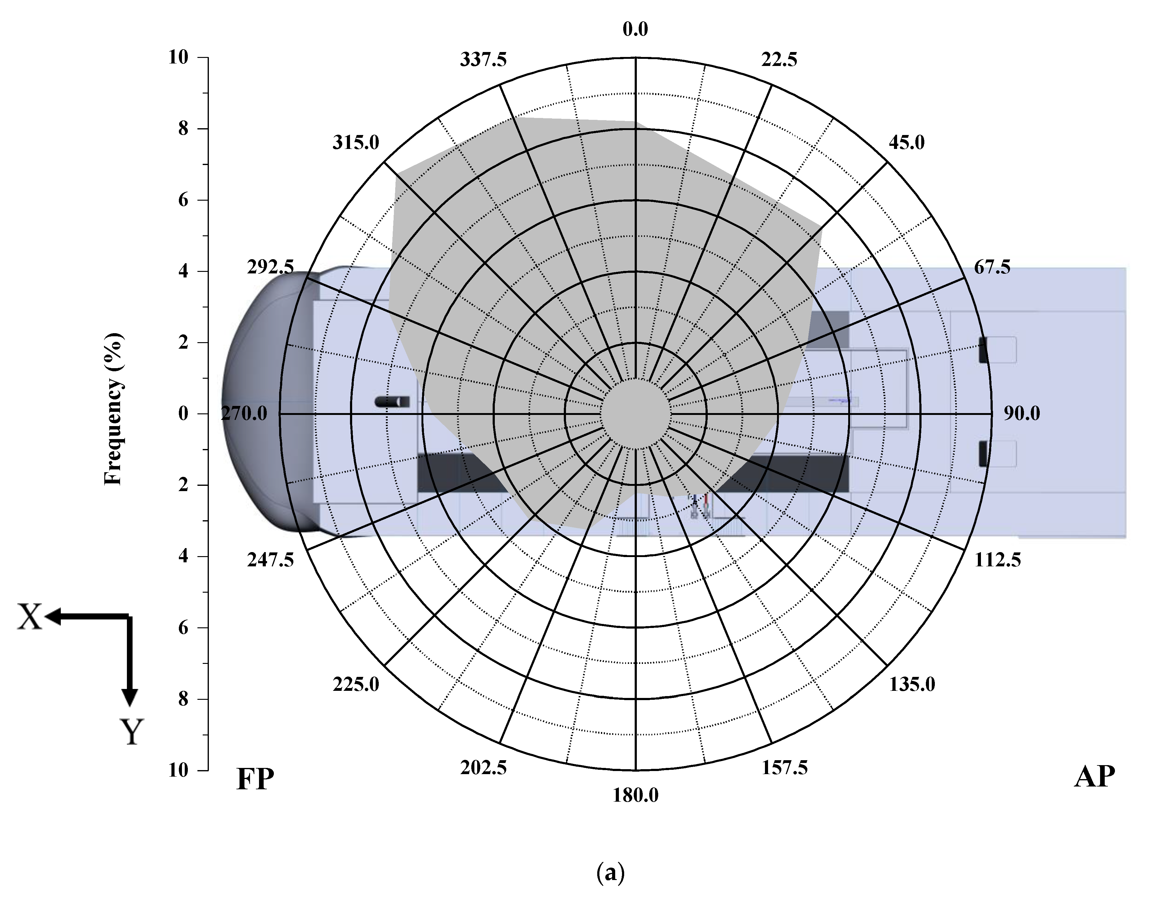
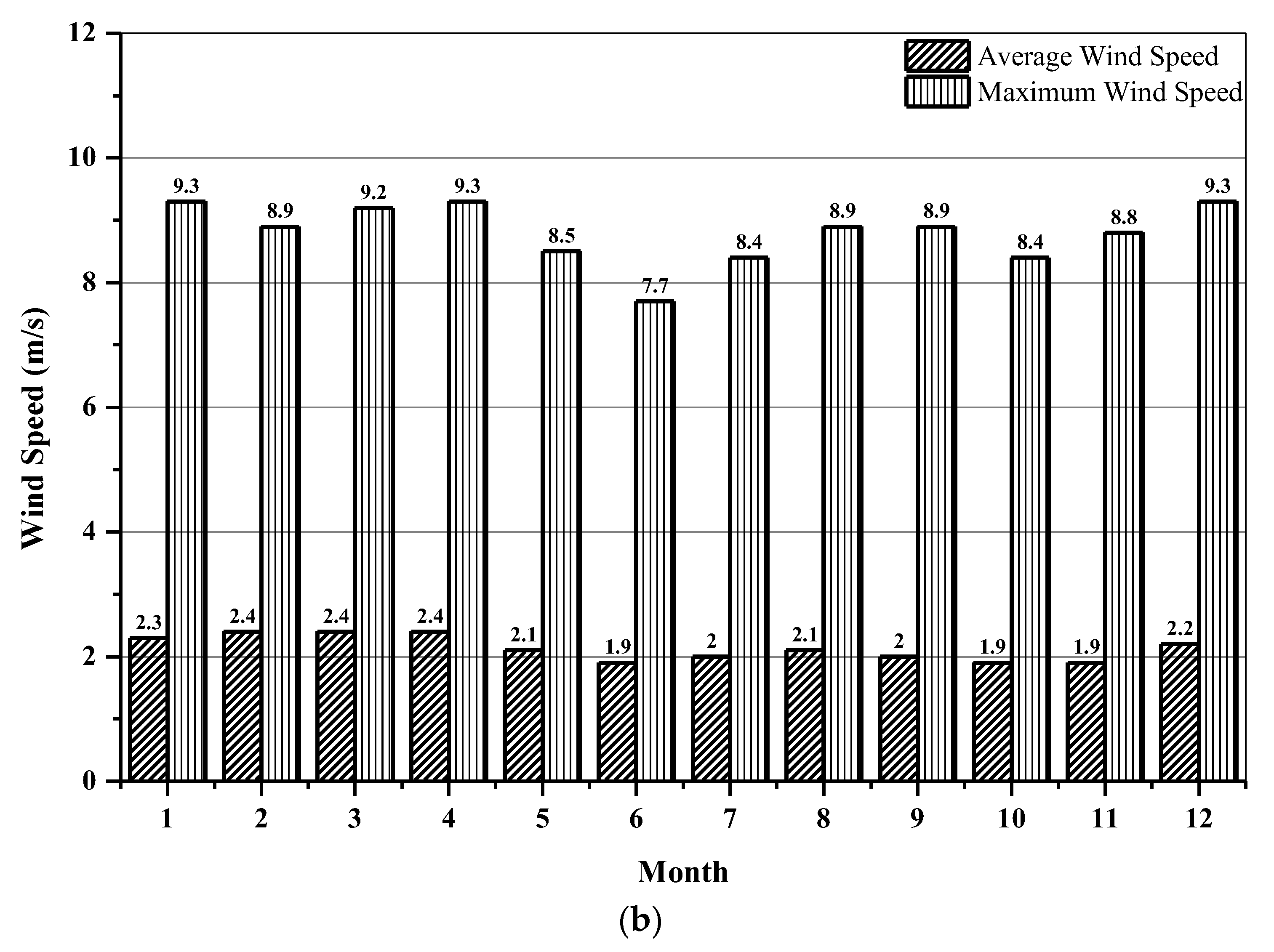
2.3. Environmental Parameters

Environmental parameters, such as wind speed, wind direction, and ambient temperature were taken into account in this study. These meteorology data were obtained at Ulsan port and prepared by the Korea Marine Equipment Research Institute (KOMERI). The wind direction data are presented as a wind rose chart that provides the wind frequencies. This frequency helps determine which variable to use. In this case, the three higher frequencies of the wind directions were selected, which were 0°, 270°, and 315°. The variables for wind speed, which were 2 m/s for the average annual wind speed and 8 m/s for the maximum annual wind speed, were selected. The annual air temperature, which was 14.95 °C, and the roughness length, which was assumed to be an open sea terrain, were also taken into account for the fixed variable. Figure 5 exhibits the wind rose chart and wind speed plot used for determining the scenario features.

2.4. LNG Leakage Scenario

The parameters for the leakage scenario were discussed and relevant data collected. All the variables considered were included to build the leakage scenario. In total, 72 different scenarios were selected, including intact and damaged geometries. Table 4 shows the parameters and variables included in the leakage scenario.

3. Technical Reference of KFX

3.1. The Standard k-ε Turbulence Model

The formation of gas clouds during LNG release is influenced by atmospheric stability. Atmospheric stability is defined as the tendency of air to displace vertically [43]. Atmospheric stability is categorized into Pasquill–Gifford stability class categories A to G, from extremely unstable to extremely stable [43,44,45]. The Pasquill–Gifford stability class describes the atmospheric stability based on estimation of the wind speed and solar radiation [43]. A stable atmosphere with low wind speed suppresses the turbulence motion and slows the mixing between natural gas and the surrounding air. Consequently, the gas is trapped near the ground at high concentration [45]. As the turbulence becomes highly non-uniform and intermittent from neutral to stable conditions, the Monin–Obukhov similarity theory provides a representation of the surface-layer mixing [45,46]. Thus, the logarithmic wind profile, which is the mean wind speed at the specific height, can be estimated [47]. The environmental parameters, such as wind speed and wind direction, are required to build the turbulence model in CFD. The vertical wind profile is also included in the turbulence model as it is related to the atmospheric stability.
A logarithmic vertical wind profile is required as KFX input to provide the vertical distribution of the horizontal mean wind speeds [48]. The equation of the logarithmic wind profile, which takes into account the Obukhov length (L) from the Monin–Obukhov similarity theory, can be used to estimate the horizontal mean wind speed (uz) as follows [49,50].
u z = u κ ln z z 0 ψ M z L + ψ M z 0 L
u z = u κ ln z d z 0
Under neutral stability conditions, Equation (3) can be applied. U denotes the friction velocity (m/s); κ is the Von Kármán constant, which is 0.41; and d is the zero-plane displacement (m), which is the height above the ground at which the zero-wind speed is achieved due to an obstacle. z denotes the elevation of wind from the ground (m); z0 denotes the roughness length (m), the approximation of which is shown in Table 5, and Ψ shows the stability term that can be expressed as follows [50]:
ψ M = 17 1 exp 0.29 z L
Table 5. Roughness length approximation based on terrain classification [49].
Terrain Classificationz0 (m)
Open sea0.0002
Mudflats, snow; no vegetation, no obstacles0.005
Open flat terrain; grass, few isolated obstacles0.03
Low crops; occasional large obstacles, x/H > 200.1
High crops; scattered obstacles, 15 < x/H < 200.25
Parkland, bushes; numerous obstacles, x/H= 100.5
Regular large obstacle coverage (suburb, forest)1
The city center with high- and low-rise buildings>2
x: typical upwind obstacle distance
H: height of the corresponding major obstacle
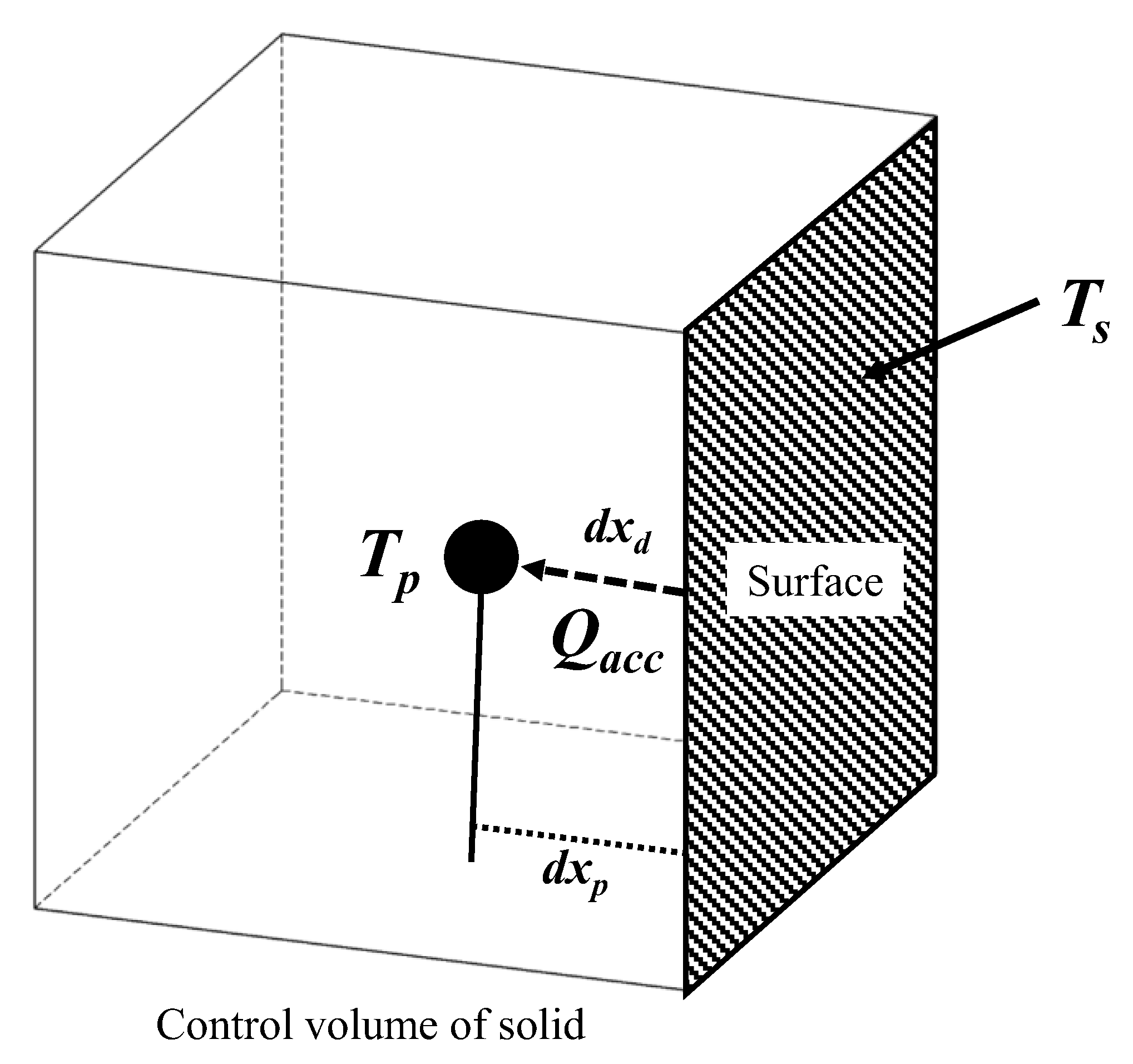
Furthermore, L can be estimated as [51]:
L = u 2 κ g θ w θ ¯
where g denotes the gravity (m/s2), θ is the potential temperature, and w′ and θ′ are perturbations of vertical velocity and virtual potential temperature. In addition, L can be described by the stability measure that is categorized into four classes, as shown in Table 6 [50]. The values of this class can be used for KFX input.
The standard k-ε turbulence model introduced by Launder and Spalding is extensively used in the CFD software [46,52]. The mechanism affecting the turbulence kinetic energy is central to this k-ε turbulence model [53]. It is assumed that convection and diffusion generate a major difference between the production and destruction of turbulence. By considering the logarithmic wind profile equation, the turbulent kinetic energy (k) (J/kg) and the dissipation rate of the turbulent kinetic energy (ε) (J/kg.s) can be written as [50,54]:
k = u 2 C D 1 z h 2
ε = u 3 κ 1 z + 4 L
The boundary layer depth (h) is the height where the velocity shear dissipates [50]. By adding the Coriolis effect (f), which is f ≈ 1.26 × 10⁻⁴ s−1 [46], h can be expressed as,
h = 0.4 u L f
An extended version of the k-ε turbulence model is adopted in KFX [41]. It is composed of the transport equation, production of k due to shear stress (P), and buoyancy (B) terms that are given in the basic version, and is expressed as follows [41,46].
ρ k t + ρ u ¯ i k x i = x i μ l + μ t σ k k x i + ρ P ρ ε + B
ρ ε t + ρ u ¯ i ε x i = x i μ l + μ t σ ε ε x i + C 1 f 1 ρ P ε k C 2 f 2 ρ ε 2 k + C 1 C 3 ε k B
A laminarization effect can be considered to occur by applying a low Reynolds number. Here, the fluid dynamic viscosity (μl), which is 0.0181 kg/m.s for air at 20 °C, and the eddy dynamic viscosity (μt) (kg/m.s) are comparable [46]. The term u ¯ is the velocity (m/s), whether in i or j components, and v denotes the kinematic viscosity (m2/s). The Cartesian coordinates are denoted as x (m), ρ is the fluid density (kg/m3), and t is time (s). Additional terms, including P and B, are expressed as follows:
P = ρ ν t u ¯ i x j + u ¯ j x i u ¯ j x i
B = Γ g i ρ x i = μ e f f σ T , t g i ρ x i
ν t = C D k 2 ε
μ e f f = μ l + μ t
where νt is the eddy kinematic viscosity (m2/s), Γ is the diffusion coefficient, σT,t is the Prandtl–Schmidt number, which is 0.7, and gi is the gravity component. The μt term is expressed as follows,
μ t = C D f μ ρ k 2 ε
f μ = exp 2.5 1 + R t / 50
R t = k 2 ν l ε = ρ k 2 μ l ε
where fμ is the correction of the low Reynolds number viscosity, Rt is the turbulent Reynolds number that is included in the correction, and νl is the fluid kinematic viscosity (m2/s) [46]. The constants that are included in the equations of the standard k-ε turbulence model are shown in Table 7.

3.2. Heat Transfer

To find the surface temperature of a solid, KFX uses the heat balance equation [41], as follows.
q r i n + q c o n v = q r o u t + q c o n d
where qrin and qrout are the radiative heat flux that is absorbed by the surface and released from the surface, respectively. qconv and qcond are the convective and conductive heat fluxes, respectively. These components can be represented as shown in Figure 6, which is located at the solid control volume.
The convective (qconv), conductive (qcond), and released radiative heat fluxes (qrout) are shown as follows,
q c o n v = h T g T s
q c o n d = k s o l d T d x s = k s o l T s T p d x p
q r o u t = α σ T s 4
where h denotes the heat transfer coefficient (W.m2.K), and Tg, Ts, and Tp are the gas temperature outside the wall, surface temperature, and temperature at the center of control volume (K), respectively. The thermal conductivity of the solid is denoted as ksol (W/m.K) which is 54 W/m.K for mild steel [55], dxp is the distance of the surface to the center of control volume (m), α is the emissivity coefficient that varies from 0 to 1, and σ is the Stefan–Boltzmann constant, which is 5.67 × 10⁸ W/m2.K4.
The heat load that enters the surface is stored inside the solid control volume as heat accumulation per surface area (qacc) in J/m2, as shown in Figure 7. qacc must be proportional to qcond [41].
Since the temperature inside the surface is a gradient, the depth of the control volume layer (dxd) in meters is considered in qacc, which can be written as [41]:
q a c c = ρ s o l C p T s T p 2 d x d
The equation includes the solid or steel density (ρsol) (kg/m3) and the specific heat capacity of steel (Cp) (J/kg.K), which is 461 J/kg.K at 20 °C [55]. Since the absorbed radiative heat flux is dominant in the fire situation over the convective heat flux, the qconv can be considered to be constant over the time step [41]. Thus, the terms qrin and qconv can be considered together as the qin term or entering heat flux. With this assumption, the heat balance equation can be written as follows,
q i n = q r o u t + q c o n d = a σ T s 4 + k s o l T s T p ρ s o l C p T s T p 2 q a c c

4. Procedure for CFD Analysis
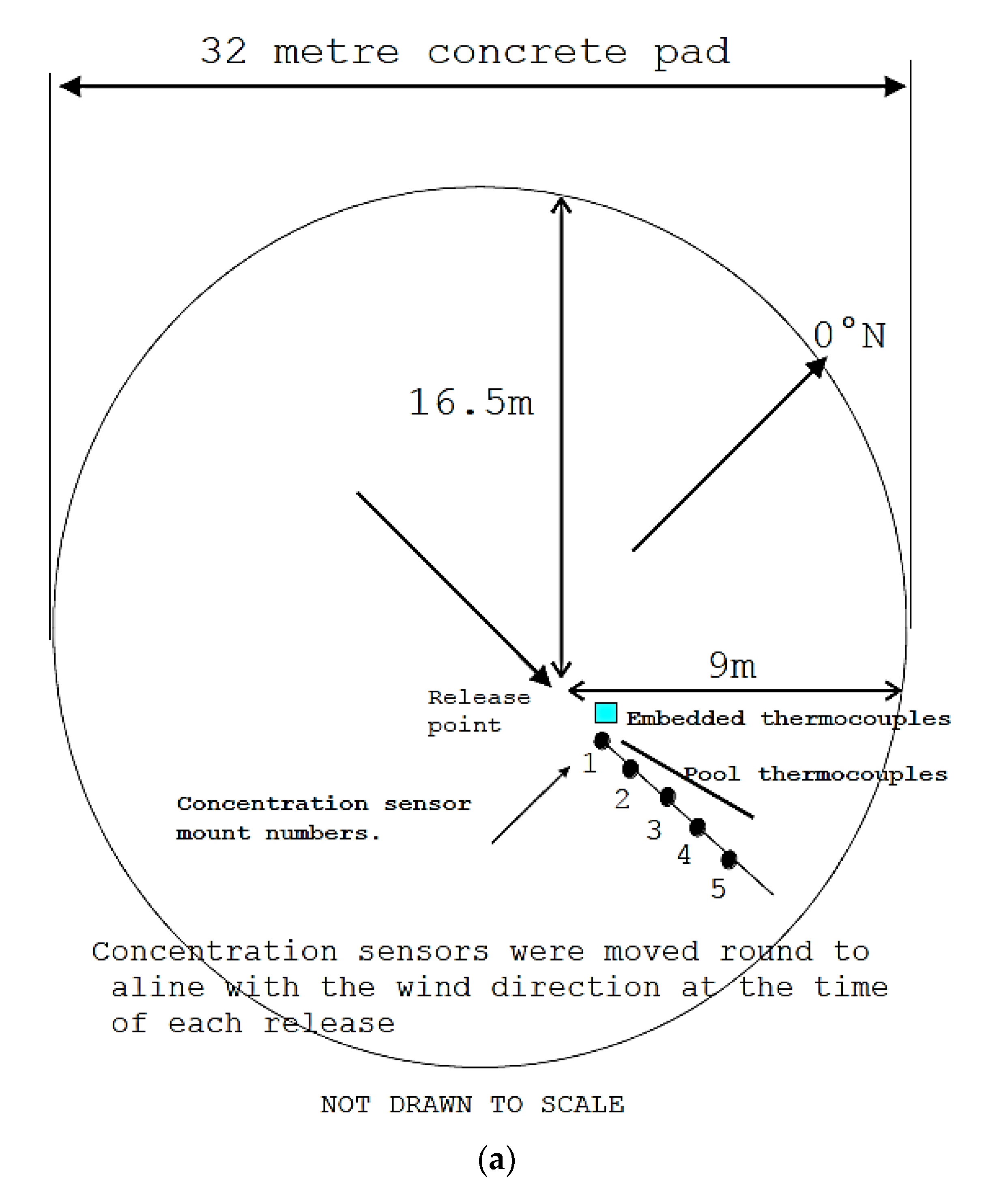
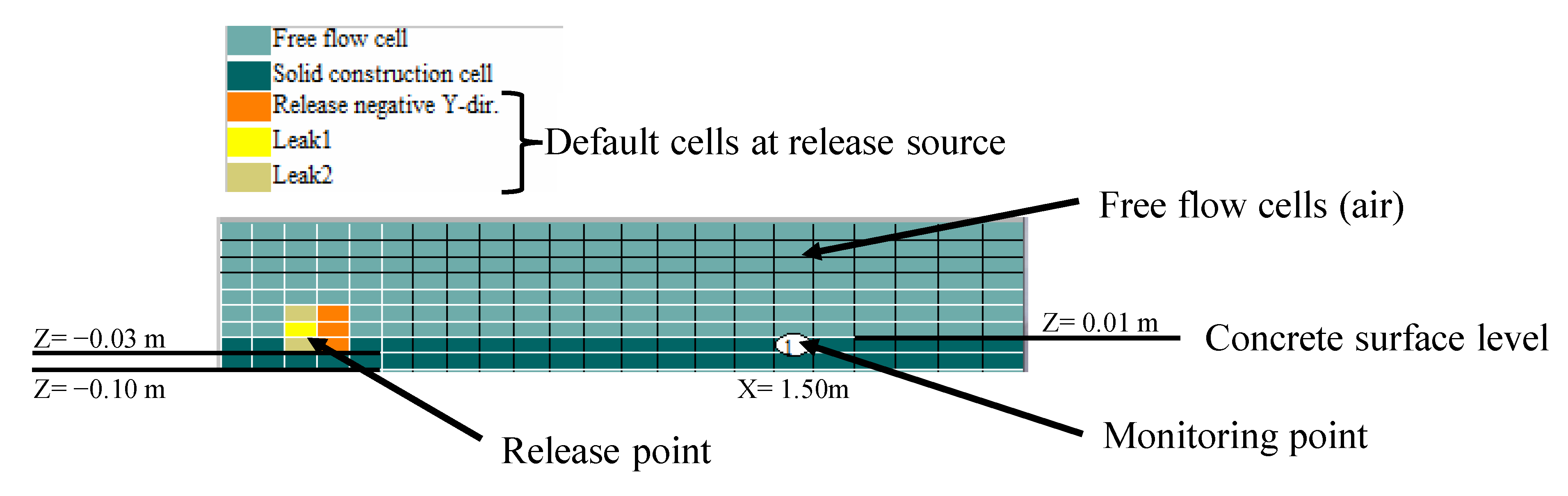
4.1. KFX Validation

A software validation was conducted before performing the main release scenario. A validation for KFX was conducted in relation to the dispersion of gas based on the British Gas experiment of large-scale gas release (1991) [18,56]. In this case, the LNG was released from the 75.00 mm hole diameter for 45 s. The wind speed was 6.80 m/s, downwind. Several sensors were installed to record the LNG concentrations along 100 m of the release path. The discrepancy in gas concentration between the experiment and the KFX model was 3.92% [18,56]. As well as hydrocarbon release, KFX can perform gas release using carbon dioxide (CO2) and hydrogen (H2). Several experimental studies of CO2 release were also conducted for KFX validation. The results showed 15.70% to 21.30% discrepancies in several of the validation assessments [22].
The KFX validations for gas dispersion cases were in good agreement since the discrepancies were slight. Another validation assessment was required to predict temperature reduction using KFX. An experimental study of liquid hydrogen (LH) release was used for validation by the UK Health and Safety Laboratory (HSL) [57]. LH was released on a concrete pad, and several thermocouples were installed at the release path, as well as embedded inside the concrete, to measure the gas and concrete temperatures. For this validation, only the embedded thermocouple data were collected. A monitoring point was marked at the solid control volume in the KFX model that worked as a thermocouple. The layout of the test rig is shown in Figure 8, illustrating the embedded thermocouples inside the concrete pad. All the embedded thermocouples were located at 1.50 m from the release point at various depths of 0.010, 0.023, and 0.027 m. The release and environmental parameters were included in the KFX model presented in Table 8. The thermal conductivity and specific heat of the concrete were 0.93 W/m.K and 880.00 J/kg.K, respectively.
Since KFX adopts the non-uniform structured Cartesian grid (NSCG) approach for generating the grid, it is difficult to determine the exact coordinates of the embedded thermocouples. Thus, the monitoring point was set to 0.003 m inside the solid control volume. Two other thermocouples were neglected due to insufficient grid instances in the KFX model. This issue demonstrates the benefits of the unstructured grid approach, which can handle arbitrary geometries, compared to the NSCG approach [58]. Figure 9 shows the release scheme for KFX representing several types of control volume or cell. The fluid domain and the solid structure were built with free flow and solid construction cells, respectively. The temperature of the concrete at the monitoring point throughout the 248 s release duration was obtained. These temperatures were compared to the LH test experiment result. Good agreement was observed as the temperature discrepancy between the test and KFX was 12.61% of the coefficient of variance (COV). Figure 10 displays a temperature plot that presents the actual temperature of the test and the KFX prediction.

4.2. Grid and Iteration Convergence Tests

These factors might impact the stability of the computation owing to discretization errors of the transport equation [59]. The control volume size and time step can be adjusted to execute the transport equation. To avoid long computation times or poor results, GCT and ICT were conducted to determine proper grid and iteration numbers. The GCT was conducted considering from 50,000 to 800,000 grids. According to the KFX manual, the computation would usually be converged at 500,000 grids [60]. To prevent the gas cloud from cascading below the waterline, the zero point of the fluid domain was placed at the ship’s waterline, which was 2.5 m from the ship’s bottom; the truncated part is shown in Figure 11. However, the consistency of results must be examined in this current model. A fixed scenario was used as input in this GCT, as well as the ICT, as shown in Table 9. In addition, 200.0 × 200.0 × 47.5 m of the fluid domain was applied, as shown in Figure 12.
The various numbers of grids and iterations can be compared with the gas cloud volume as a physical parameter, as provided by the results of the GCT and ICT. Figure 12a presents a plot of the gas cloud volume versus the number of grids. Here, the results for gas cloud volume converged at 200,000 grids. However, to ensure a stable result and to save computation time, 600,000 grids were selected for the main scenario. It was found that the discrepancy between 200,000 and 800,000 grids, which produced a stable result, was only 6.40% of the COV. The result of the ICT is shown in Figure 12b. The ICT was conducted with the iteration variable ranging from 30 to 1500 iterations. The 600,000 grids selected were applied to the ICT. This iteration number was used to define the time step in the simulation. In this case, the simulation duration was 15 s, which was then divided by the iteration number to obtain the time step. Here, 500 iterations were selected for the same reason as the GCT result. With the current iteration number, 0.03 s of time step was able to be used in the main simulation.

5. Parametric Study on Intact and Damaged Geometries

5.1. Gas Dispersion

The main leakage scenarios were simulated in KFX—one of the objectives was to establish the critical zone. The safety or critical zone is the area where the ignition source and non-essential personnel are controlled, and only dedicated activities are allowed [7,29,60]. This zone has to be established around the bunkering station or facilities and may be applied when the LNG cargo is being loaded or unloaded [7]. The critical zone can be determined by predicting the distance at which a gas cloud with a concentration above LFL is dispersed [29,60]. For safety reasons, several past studies have applied the critical zone measurement based on half LFL to the upper flammability limit (UFL) threshold [18,25,26,27,61,62].
Here, every scenario that applied 50 mm leak diameters had a significant amount of released gas, as shown in Figure 13 and Figure 14, compared to the 3 and 10 mm leak diameters, as shown in Figure 15 and Figure 16. Thus, wind conditions have a major effect on these 50 mm leakages. These gas contour plots were used to measure the distance of the released gas. The scenario nomenclature contrasts In and Dm, which represent intact and damaged geometries, respectively. Thus, a scenario with the same variables except for the geometric condition was unified with the same numbering for data simplification. Table 10 shows a summary of the critical zone and gas cloud volume for all scenarios.
Generally, the gas cloud formation was significantly affected by the wind conditions and obstacles near to the release point. In this case, the release in the pipe had a larger gas cloud volume than the release in the valve. This was due to the position of the pipe leak located in the front of the stern trunk wall. Thus, the gas flows were reflected and re-entrained to the release path. This decelerated dissipation of the gas cloud. Because the LNG had not yet vaporized in the entrainment zone, the gas accumulation caused a rainout [43,63]. Figure 17 shows the typical gas cloud formation for leakages both from the valve and pipe. Here, the release in the valve showed a longer gas path and a wider shape of the pipe leakage. Figure 18 shows the gas cloud volume in each wind direction of the valve and pipe leakage. The plots show that a mild wind speed of 2 m/s had a larger gas cloud volume than for a wind speed of 8 m/s, with neutral atmospheric stability in all cases. With mild wind, the gas was dispersed slowly, resulting in an accumulation of gas near the release point, resulting in the buildup of a higher concentration of gas. On the other hand, the higher wind speed accelerated the dissipation of gas, causing mixing with the air to form a lower concentration of gas. Furthermore, a larger gas cloud volume was often present in cases with a wind direction of 360°. This indicated the buildup of gas on the ship’s port side, particularly near the bunkering station. A substantial quantity of gas cloud particles fell into the bunkering station. The cargo hold construction also obstructed the wind flow. Consequently, there was a significant gas pocket here.
The intact ship caused a larger gas accumulation than the damaged ship due to the existence of the bunkering station structure. It slowed down the gas dissipation in the bunkering station region because the wind flow was also slower here. In the damaged ship, the gas cloud dissipated faster in the bunkering station. The wind velocity was slightly slower in sc.In.33 than sc.Dm.33 located on the bunkering station, as shown in Figure 19b. As shown in Figure 19a, the gas cloud had a thinner shape on the damaged ship than on the intact ship around the port side of the bunkering station. This was clearly evident at the bunkering station. Furthermore, in the damaged condition, there was an absence of bunkering station structure, and some side shell structures on the port side. The gas cloud did not expose the storage tank inside. For the damaged ship, the gas cloud was ejected far from the port side or dissipated rapidly with stronger wind speed. Though there was a different amount of gas cloud accumulation between intact and damaged ships, the discrepancy in gas cloud volume was not large. Neglecting the gas cloud volume for the 3 and 10 mm cases, the COV between the intact and damaged cases was 25.56%. Figure 20 presents a plot of the gas cloud volume for the intact and damaged ship.

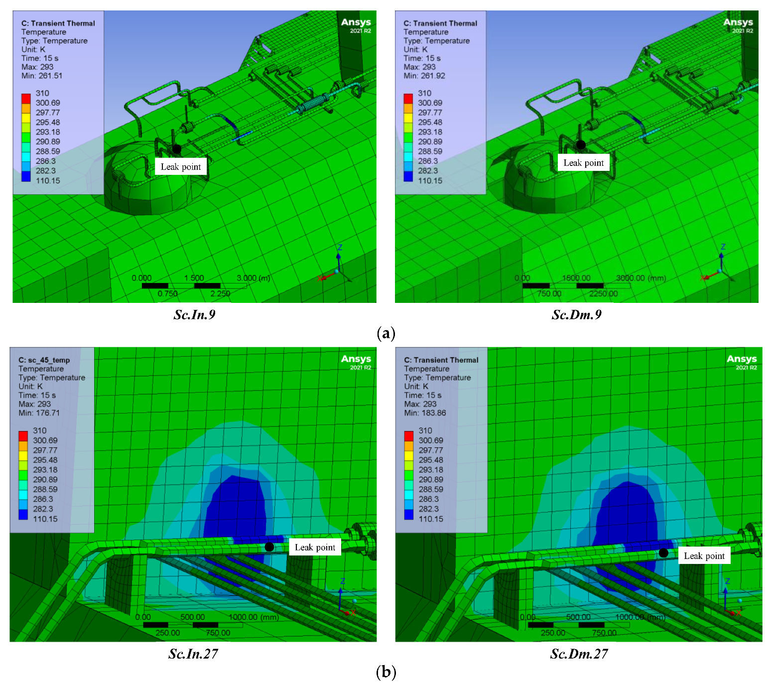
5.2. Temperature Reduction

To observe the temperature reduction due to gas exposure, gas temperature plots are shown in Figure 21, which were taken from Sc.In/Dm.9 and Sc.In/Dm.27. The contour of these plots ranged from 110.15 (−163.00 °C) to 273.15 K (0.00 °C). The valve leakage shows that the cold gas significantly exposed a pipe in front of the leak point. It reached the stern trunk wall, but the gas temperature expanded to around 0.00 °C at the trunk wall. Thus, it could not lead to a significant temperature reduction in the ship’s structure, except for the equipment near the leak point. However, the pipe leakage led to a major temperature reduction on the stern trunk wall due to its leak position. As explained previously, the gas flow of this leakage was directly exposed to the stern trunk wall, and the gas cloud accumulated here. The gas temperature on the surface of the stern trunk wall was lower than 142.75 K or −130.40 °C, as shown in the plot of Figure 21b. Overall, the gas temperature plots show that the cold gas did not reach the inside of the cargo hold. Thus, the cold gas exposure between the intact and damaged ships was similar to that in the other scenarios.
Steel temperature plots can be used to detect the cold gas effect on the structure. The steel temperature profiles from KFX were transferred to the FE software, ANSYS/LS-DYNA. The data for the temperature profile consist of the steel temperature at each coordinate point of the grids. These coordinate points can be read as the node points in ANSYS/LS-DYNA. By providing the same position and dimension of the ship model in KFX and ANSYS/LS-DYNA, the temperature profile can be easily transferred. This temperature profile can be used as the loads for the structural strength analysis in further studies. The steel temperature plot can be created easily in FE software. Figure 22 shows plots of the steel temperature showing leakages from the valve and pipe. Instances of valve leakage only exposed the equipment in front of the leak point, such as pipes and other valves. In instances of pipe leakage, the gas significantly exposed the stern trunk wall, in proportion to the gas temperature. Overall, the steel temperature can be predicted according to the values shown in Table 11, which were taken from the results for Sc.In/Dm.9 and Sc.In/Dm.27.
A comparison of the steel temperature between the intact and damaged ships is also provided. Figure 23 presents steel temperature plots for the entire scenario. Here, the steel temperature discrepancy between the intact and damaged ships was insignificant since the cold gas did not expose the damaged part of the ship. Locations that were exposed to the cold gas were similar for the intact and damaged ships. Discrepancies of the steel temperature only reached 1.98% of the COV in all cases.

6. Conclusions

This paper offers a consequence analysis for an LNG bunkering ship in the event of an accidental LNG release, considering both intact and damaged conditions. A previous ship collision study was utilized to define the wrecked part for the damaged ship. The procedure for determining the LNG leakage scenario is presented, and the leakage and environment parameters are considered. Data from the previous collision study on depth penetration were utilized to build the ship’s geometry. Several variables, such as leak diameter, wind speed, wind direction, and depth penetration, were defined by considering their frequencies, to obtain a credible leakage scenario. A total of 72 scenarios were generated in the study.
Grid and iteration convergence tests were conducted to obtain adequate numbers of grids and iterations used for the main CFD analysis. A KFX validation is presented, using a UK HSL liquid hydrogen release experiment, which was modeled in KFX. The validation produced a satisfactory result in which the discrepancy for the solid temperature between the KFX and UK HSL test did not reach 15% of the COV. With respect to the results of the CFD analysis, key points are summarized below:
  • The gas dispersion characteristics are inferred from the gas cloud volume and its shape. The wind and obstructions exert the main influence on the formation of the gas cloud. The CFD result shows that the leakage in the pipe involves a large accumulation of gas due to its position near an obstacle that causes the released gas to be re-entrained into the release path. For leakage in the valve, the gas cloud can be easily dissipated and mixed with the air since there is no significant obstacle to disturb its release path.
  • The steel temperature reduces significantly in the stern trunk wall as a result of leakages from the pipe. The cold gas exposes this section due to the leak point adjacent to the stern trunk wall. For leakages from the valve, the cold gas was already expanded when it reached the stern trunk wall. Thus, the temperature reduction in this case was minor. Overall, the cold gas did not reach the broken part of the damaged ship, which was inside the cargo hold. As a result, there was no major difference in the cooling effect between the intact and damaged ships.
  • A profile of steel temperature was retrieved from KFX to ANSYS/LS-DYNA. The temperature reduction was significant for the leakages from the pipe, and was typically below 200 K for a 50 mm leak diameter. Since the cold gas was built adjacent to the leak point, it had no noticeable impact on the ship’s structure for 3 and 10 mm leak diameters.
This study is limited in only assessing simulation of gas dispersion to obtain the steel temperature profile. Pipe leakages with 50 mm leak diameter represent interesting cases for future structural strength analysis using FE since the cryogenic flow in these cases severely exposed the structure of the stern trunk wall. This part must be checked for indications of cracks or embrittlement due to the cooling effect, using finite element analysis.

Author Contributions

Conceptualization, J.-M.S. and H.N.; methodology, J.-M.S. and H.N.; software, H.N.; validation, H.N.; formal analysis, H.N.; investigation, J.-M.S. and H.N.; resources, J.-M.S. and D.J.; data curation J.-M.S. and H.N.; writing—original draft preparation, H.N.; writing—review and editing, J.-M.S. and H.N.; visualization, H.N.; supervision, J.-M.S.; project administration, J.-M.S.; funding acquisition, J.-M.S. All authors have read and agreed to the published version of the manuscript.

Funding

This research was funded by the Ministry of Ocean and Fisheries of South Korea, grant number “PMS5290”. The APC was funded under a grant of “BK21 FOUR MADEC” from the Marine Designeering Education Research Group, South Korea.

Institutional Review Board Statement

Not applicable.

Informed Consent Statement

Not applicable.

Data Availability Statement

Not applicable.

Acknowledgments

This work is a result of the project, ‘Development of LNG Bunkering Operation Technologies based on Operation System and Risk Assessment (PMS5290)’ supported by the Ministry of Ocean and Fisheries in South Korea. The first author gratefully acknowledges financial support under the grant of Brain Korea 21 Program for Leading Universities and Students (BK21 FOUR MADEC) from the Marine Designeering Education Research Group, South Korea.

Conflicts of Interest

The authors declare no conflict of interest. The funders had no role in the design of the study; in the collection, analyses, or interpretation of data; in the writing of the manuscript; or in the decision to publish the results.

References

  1. International Maritime Organization. Resolution MEPC.203(62)—Amendments to the Annex of the Protocol of 1997 to Amend the International Convention for the Prevention of Pollution from Ships, 1973, as Modified by the Protocol of 1978 Relating Thereto (Inclusion of Regulations on Energy Effi). 2011. Available online: https://wwwcdn.imo.org/localresources/en/OurWork/Environment/Documents/Technical%20and%20Operational%20Measures/Resolution%20MEPC.203%2862%29.pdf (accessed on 20 September 2022).
  2. Martinsen, K. Alternative Fuels Insight. Available online: https://www.dnv.com/services/alternative-fuels-insight-128171 (accessed on 20 September 2022).
  3. Le Fevre, C. A Review of Demand Prospects for LNG as a Marine Transport Fuel; The Oxford Institute for Energy Studies: Oxford, UK, 2018; ISBN 9781784671143. [Google Scholar]
  4. Park, N.K.; Park, S.K. A Study on the Estimation of Facilities in LNG Bunkering Terminal by Simulation—Busan Port Case. J. Mar. Sci. Eng. 2019, 7, 354. [Google Scholar] [CrossRef]
  5. Tam, J.H. Overview of Performing Shore-to-Ship and Ship-to-Ship Compatibility Studies for LNG Bunker Vessels. J. Mar. Eng. Technol. 2020, 21, 257–270. [Google Scholar] [CrossRef]
  6. Park, S.; Jeong, B.; Yoon, J.Y.; Paik, J.K. A Study on Factors Affecting the Safety Zone in Ship-to-Ship LNG Bunkering. Ships Offshore Struct. 2018, 13, 312–321. [Google Scholar] [CrossRef]
  7. Maritime Safety Agency (EMSA). Guidance on LNG Bunkering to Port Authorities and Administrations; EMSA: Lisbon, Portugal, 2018.
  8. Ahn, J.; Choi, Y.; Jo, C.; Cho, Y.; Chang, D.; Chung, H.; Bergan, P.G. Design of a Prismatic Pressure Vessel with Internal X-Beam Structures for Application in Ships. Ships Offshore Struct. 2017, 12, 781–792. [Google Scholar] [CrossRef]
  9. Kim, J.-W.; Jeong, J.; Chang, D.-J. Optimal Shape and Boil-Off Gas Generation of Fuel Tank for LNG Fueled Tugboat. J. Ocean. Eng. Technol. 2020, 34, 19–25. [Google Scholar] [CrossRef]
  10. Oh, S.; Jung, D.-W.; Kim, Y.-H.; Kwak, H.-U.; Jung, J.-H.; Jung, S.-J.; Park, B.; Cho, S.-K.; Jung, D.; Sung, H.G. Numerical Study on Characteristics and Control of Heading Angle of Floating LNG Bunkering Terminal for Improvement of Loading and Off-Loading Performance. J. Ocean. Eng. Technol. 2020, 34, 77–88. [Google Scholar] [CrossRef]
  11. Vanem, E.; Antão, P.; Østvik, I.; de Comas, F.D.C. Analysing the Risk of LNG Carrier Operations. Reliab. Eng. Syst. Saf. 2008, 93, 1328–1344. [Google Scholar] [CrossRef]
  12. European Commission. EMARS: Electronic Major Accident Report System. Available online: https://emars.jrc.ec.europa.eu/en/emars/content (accessed on 20 September 2022).
  13. Pujol, J.; Kleiveland, R.N.; Lileheie, N.I.; Holmas, T.; Amdahl, J. Advanced Cryogenic Structural Collapse Analysis CSCA—Part II: Cryogenic Flow and Structural Cooling. In Proceedings of the Offshore Technology Conference Asia, Kuala Lumpur, Malaysia, 22–25 March 2016; OnePetro: Richardson, TX, USA, 2016; pp. 108–115. [Google Scholar] [CrossRef]
  14. Paik, J.K.; Kim, B.J.; Jeong, J.S.; Kim, S.H.; Jang, Y.S.; Kim, G.S.; Woo, J.H.; Kim, Y.S.; Chun, M.J.; Shin, Y.S.; et al. CFD Simulations of Gas Explosion and Fire Actions. Ships Offshore Struct. 2010, 5, 3–12. [Google Scholar] [CrossRef]
  15. Jujuly, M.M.; Rahman, M.; Ahmed, S.; Khan, F. LNG Pool Fire Simulation for Domino Effect Analysis. Reliab. Eng. Syst. Saf. 2015, 143, 19–29. [Google Scholar] [CrossRef]
  16. Fu, S.; Yan, X.; Zhang, D.; Li, C.; Zio, E. Framework for the Quantitative Assessment of the Risk of Leakage from LNG-Fueled Vessels by an Event Tree-CFD. J. Loss Prev. Process Ind. 2016, 43, 42–52. [Google Scholar] [CrossRef]
  17. Baalisampang, T.; Abbassi, R.; Garaniya, V.; Khan, F.; Dadashzadeh, M. Accidental Release of Liquefied Natural Gas in a Processing Facility: Effect of Equipment Congestion Level on Dispersion Behaviour of the Flammable Vapour. J. Loss Prev. Process Ind. 2019, 61, 237–248. [Google Scholar] [CrossRef]
  18. Nubli, H.; Sohn, J.M. CFD-Based Simulation of Accidental Fuel Release from LNG-Fuelled Ships. Ships Offshore Struct. 2020, 17, 339–358. [Google Scholar] [CrossRef]
  19. Nubli, H.; Sohn, J.M. Procedure for Determining Design Accidental Loads in Liquified-Natural-Gas-Fuelled Ships under Explosion Using a Computational-Fluid-Dynamics-Based Simulation Approach. Ships Offshore Struct. 2021, 1–18. [Google Scholar] [CrossRef]
  20. Nubli, H.; Sohn, J.M.; Prabowo, A.R. Layout Optimization for Safety Evaluation on LNG-Fueled Ship under an Accidental Fuel Release Using Mixed-Integer Nonlinear Programming. Int. J. Nav. Arch. Ocean Eng. 2022, 14, 100443. [Google Scholar] [CrossRef]
  21. Magnussen, B.F. On the Structure of Turbulence and a Generalized Eddy Dissipation Concept for Chemical Reaction in Turbulent Flow. In Proceedings of the 19th Aerospace Sciences Meeting, St. Louis, MO, USA, 12–15 January 1981; American Institute of Aeronautics and Astronautics: Reston, VA, USA, 1981. [Google Scholar]
  22. Rian, K.E.; Grimsmo, B.; Lakså, B.; Vembe, B.E.; Lilleheie, N.I.; Brox, E.; Evanger, T. Advanced CO2 Dispersion Simulation Technology for Improved CCS Safety. Energy Procedia 2014, 63, 2596–2609. [Google Scholar] [CrossRef]
  23. Hansen, O.R.; Gavelli, F.; Ichard, M.; Davis, S.G. Validation of FLACS against Experimental Data Sets from the Model Evaluation Database for LNG Vapor Dispersion. J. Loss Prev. Process Ind. 2010, 23, 857–877. [Google Scholar] [CrossRef]
  24. Society of Gas as a Marine Fuel. Gas as a Marine Fuel, Safety Guidelines; Bunkering: London, UK, 2017. [Google Scholar]
  25. Webber, D.M.; Ivings, M.J.; Santon, R.C. Ventilation Theory and Dispersion Modelling Applied to Hazardous Area Classification. J. Loss Prev. Process Ind. 2011, 24, 612–621. [Google Scholar] [CrossRef]
  26. Havens, J.; Spicer, T. LNG Vapor Cloud Exclusion Zones for Spills into Impoundments. Process Saf. Prog. 2005, 24, 181–186. [Google Scholar] [CrossRef]
  27. Cormier, B.R.; Qi, R.; Yun, G.W.; Zhang, Y.; Mannan, M.S. Application of Computational Fluid Dynamics for LNG Vapor Dispersion Modeling: A Study of Key Parameters. J. Loss Prev. Process Ind. 2009, 22, 332–352. [Google Scholar] [CrossRef]
  28. Nubli, H.; Prabowo, A.R.; Sohn, J.M. Gas Dispersion Analysis on the Open Deck Fuel Storage Configuration of the LNG-Fueled Ship. In Proceedings of the 6th International Conference and Exhibition on Sustainable Energy and Advanced Materials—Lecture Notes in Mechanical Engineering, Surakarta, Indonesia, 16–17 October 2019; pp. 109–118. [Google Scholar] [CrossRef]
  29. Park, S.I.; Paik, J.K. A Hybrid Method for the Safety Zone Design in Truck-to-Ship LNG Bunkering. Ocean Eng. 2022, 243, 110200. [Google Scholar] [CrossRef]
  30. International Organization for Standardization. Guidelines for Safety and Risk Assessment of LNG Fuel Bunkering Operations. Switzerland. 2021. Available online: https://www.iso.org/obp/ui/fr/#iso:std:iso:ts:18683:ed-2:v1:en (accessed on 20 September 2022).
  31. Lloyd’s Register. Guidance Notes for Risk Based Analyses; Cryogenic Spill: London, UK, 2015. [Google Scholar]
  32. Paik, J.K.; Lee, D.H.; Noh, S.H.; Park, D.K.; Ringsberg, J.W. Full-Scale Collapse Testing of a Steel Stiffened Plate Structure under Axial-Compressive Loading Triggered by Brittle Fracture at Cryogenic Condition. Ships Offshore Struct. 2020, 15, S29–S45. [Google Scholar] [CrossRef]
  33. Han, S.; Bae, J.; Joh, K.; Suh, Y.; Eom, J.K. Assessing Structural Safety of Inner Hull Structure under Cryogenic Temperature. In Proceedings of the International Conference on Offshore Mechanics and Arctic Engineering—OMAE, Rotterdam, The Netherlands, 19–24 June 2011; Volume 2, pp. 961–967. [Google Scholar]
  34. Petti, J.P.; Lopez, C.; Figueroa, V.; Kalan, R.J.; Wellman, G.; Dempsey, J.; Villa, D.; Hightower, M. LNG Vessel Cascading Damage Structural and Thermal Analyses. IGT Int. Liq. Nat. Gas Conf. Proc. 2013, 2, 899–922. [Google Scholar]
  35. Carvalho, E.D.; Marcer, R.; Audiffren, C.; Ciotat, L. Experimental Tests and Qualification of a CFD Simulation Tool for Cryogenic Release Modelling through the JIP “FLNG Cryogenic Spillage Protection. In Proceedings of the Gas Processors Association Europe—2017 Annual Conference, Budapest, Hungary, 13–16 September 2017. [Google Scholar]
  36. Xie, C.; Huang, L.; Wang, R.; Deng, J.; Shu, Y.; Jiang, D. Research on Quantitative Risk Assessment of Fuel Leak of LNG-Fuelled Ship during Lock Transition Process. Reliab. Eng. Syst. Saf. 2022, 221, 108368. [Google Scholar] [CrossRef]
  37. Peng, Y.; Zhao, X.; Zuo, T.; Wang, W.; Song, X. A Systematic Literature Review on Port LNG Bunkering Station. Transp. Res. Part D Transp. Environ. 2021, 91, 102704. [Google Scholar] [CrossRef]
  38. Sohn, J.M.; Jung, D. Structural Assessment of a 500-Cbm Liquefied Natural Gas Bunker Ship during Bunkering and Marine Operation under Collision Accidents. Ships Offshore Struct. 2021, 1–17. [Google Scholar] [CrossRef]
  39. Davies, P.A.; Fort, E. LNG as a Marine Fuel: Likelihood of LNG Releases. J. Mar. Eng. Technol. 2013, 12, 3–10. [Google Scholar] [CrossRef]
  40. IOGP. Risk Assessment Data Directory—Process Release Frequencies (IOGP Report 434-01); International Association of Oil and Gas Producers: London, UK, 2019. [Google Scholar]
  41. Vembe, B.E.; Rian, K.E.; Holen, J.; Lilleheie, N.I.; Grimsmo, B. Kameleon FireEx 2000 (Theory Manual); Computit: Brisbane, Australia, 2001. [Google Scholar]
  42. Fernández, I.A.; Gómez, M.R.; Gómez, J.R.; Insua, Á.B. Review of Propulsion Systems on LNG Carriers. Renew. Sustain. Energy Rev. 2017, 67, 1395–1411. [Google Scholar] [CrossRef]
  43. Woodward, J.L. Estimating the Flammable Mass of a Vapor Cloud; Wiley: New York, NY, USA, 1999; ISBN 978-0-816-90778-6. [Google Scholar]
  44. NOAA. Pasquill Stability Classes. Available online: https://www.ready.noaa.gov/READYpgclass.php (accessed on 15 July 2022).
  45. Luketa-Hanlin, A.; Koopman, R.P.; Ermak, D.L. On the Application of Computational Fluid Dynamics Codes for Liquefied Natural Gas Dispersion. J. Hazard. Mater. 2007, 140, 504–517. [Google Scholar] [CrossRef]
  46. Bærland, T. Release and Spreading of Dense Gases: Turbulence Modeling with Kameleon FireEx. Master’s Thesis, Norwegian University of Science and Technology, Trondheim, Norway, 2011. [Google Scholar]
  47. Ro, K.S.; Hunt, P.G. Characteristic Wind Speed Distributions and Reliability of the Logarithmic Wind Profile. J. Environ. Eng. 2007, 133, 313–318. [Google Scholar] [CrossRef]
  48. Oke, T.R. Boundary Layer Climates, 2nd ed.; Routledge: Abingdon-on-Thames, UK, 1987; Volume 7, ISBN 0203715454. [Google Scholar]
  49. Van Ulden, A.P.; Holtslag, A.A.M. Estimation of Atmospheric Boundary Layer Parameters for Diffusion Applications. J. Clim. Appl. Meteorol. 1985, 24, 1196–1207. [Google Scholar] [CrossRef]
  50. Huser, A.; Nilsen, P.J.; Skåtun, H. Application of K-ε Model to the Stable ABL: Pollution in Complex Terrain. J. Wind Eng. Ind. Aerodyn. 1997, 67–68, 425–436. [Google Scholar] [CrossRef]
  51. Foken, T. Micrometeorology; Springer: Berlin/Heidelberg, Germany, 2008; ISBN 978-3-540-74665-2. [Google Scholar]
  52. Launder, B.E.; Spalding, D.B. The Numerical Computation of Turbulent Flows. Comput. Methods Appl. Mech. Eng. 1974, 3, 269–289. [Google Scholar] [CrossRef]
  53. Versteeg, H.K.; Malalasekera, W. An Introduction to Computational Fluid Dynamics: The Finite Volume Method, 2nd ed.; Pearson Education Limited: Harlow, UK, 2007; ISBN 978031274983. [Google Scholar]
  54. Duynkerke, P.G. Application of the E-ϵ Turbulence Closure Model to the Neutral and Stable Atmospheric Boundary Layer. J. Atmos. Sci. 1988, 45, 865–880. [Google Scholar] [CrossRef]
  55. Thysenkrupp Material Data Sheet. Available online: https://ucpcdn.thyssenkrupp.com/_legacy/UCPthyssenkruppBAMXFrance/assets.files/product_pdf/carbon_flat_steel_/plates_and_slabs_carbon_steel/s235jr_1_0038_11_2016_engl.pdf (accessed on 8 August 2022).
  56. Rian, K.E.; Vembe, B.E.; Evanger, T. KFX Validation Handbook; ComputIT: Trondheim, Norway, 2016. [Google Scholar]
  57. Royle, M.; Willoughby, D.B. Release of Unignited Liquid Hydrogen; IGEM: Buxton, UK, 2014. [Google Scholar]
  58. Manchester CFD. All There Is to Know about Different Mesh Types in CFD! Available online: https://www.manchestercfd.co.uk/post/all-there-is-to-know-about-different-mesh-types-in-cfd (accessed on 10 July 2022).
  59. NASA. Examining Spatial (Grid) Convergence. Available online: www.grc.nasa.gov/www/wind/valid/tutorial/spatconv.html (accessed on 25 July 2022).
  60. Vembe, B.E.; Kleiveland, R.N.; Grimsmo, B.; Lilleheie, N.I.; Rian, K.E.; Olsen, R.; Lakså, B.; Nilsen, V.; Vembe, J.E.; Evanger, T. KFX—User’s Manual; Computit: Trondheim, Norway, 2017. [Google Scholar]
  61. Ennis, A. Development of Source Terms for Gas Dispersion and Vapour Cloud Explosion Modelling. In Institution of Chemical Engineers Symposium Series; Institution of Chemical Engineers: Rugby, UK, 2006; p. 108. [Google Scholar]
  62. Shao, H.; Duan, G. Risk Quantitative Calculation and ALOHA Simulation on the Leakage Accident of Natural Gas Power Plant. Procedia Eng. 2012, 45, 352–359. [Google Scholar] [CrossRef]
  63. Lim, B.H.; Ng, E.Y.K. Model for Cryogenic Flashing Lng Leak. Appl. Sci. 2021, 11, 9312. [Google Scholar] [CrossRef]
Figure 1. A framework for temperature reduction analysis.
Jmse 10 01378 g001
Figure 2. Frequency of penetration distance.
Jmse 10 01378 g002
Figure 3. Initial (a), damaged geometries (b) and cut view (c) of the LNG bunkering ship model.
Jmse 10 01378 g003
Figure 4. Two leak positions in the fuel supply deck of the LNG bunkering system.
Jmse 10 01378 g004
Figure 5. (a) Wind rose chart and (b) wind speed plots at Ulsan port.
Jmse 10 01378 g005aJmse 10 01378 g005b
Figure 6. Heat balance diagram.
Jmse 10 01378 g006
Figure 7. Heat transfer on the solid control volume.
Jmse 10 01378 g007
Figure 8. The layout of the test rig with Embedded and Pool thermocouples (marked with cyan square and black dots, respectively) (a) and embedded thermocouples (b) [57].
Jmse 10 01378 g008aJmse 10 01378 g008b
Figure 9. Scheme of LH release in KFX.
Jmse 10 01378 g009
Figure 10. Plot of test temperature and KFX prediction.
Jmse 10 01378 g010
Figure 11. Section of the fluid domain and target ship with 600,000 grids: top view (a) and side view (b).
Jmse 10 01378 g011aJmse 10 01378 g011b
Figure 12. Plots of gas cloud volume versus number of grids (a) and iteration numbers (b).
Jmse 10 01378 g012aJmse 10 01378 g012b
Figure 13. Gas contour plot for the 50 mm valve leak at (a,b) 2 m/s and (c,d) 8 m/s wind speed. The wind direction is symbolized as an arrow at the right bottom of the plot.
Jmse 10 01378 g013aJmse 10 01378 g013b
Figure 14. Gas contour plot for the 50 mm pipe leak at (a,b) 2 m/s and (c,d) 8 m/s wind speed.
Jmse 10 01378 g014aJmse 10 01378 g014b
Figure 15. Gas contour plot for the 10 mm valve leak at 2 m/s for (a) intact and (b) damaged ships.
Jmse 10 01378 g015
Figure 16. Gas contour plot for the 3 mm valve leak at 2 m/s for (a) intact and (b) damaged ships.
Jmse 10 01378 g016
Figure 17. Typical gas cloud formation of gas release from valve and pipe.
Jmse 10 01378 g017
Figure 18. Plots of gas cloud volume with respect to wind direction: release in valve (a) and release in the pipe (b).
Jmse 10 01378 g018
Figure 19. The combined wind velocity (wind direction is marked as arrows) and gas concentration plots of 2 m/s (a) and 8 m/s wind speed (b).
Jmse 10 01378 g019
Figure 20. Plot of gas cloud volume.
Jmse 10 01378 g020
Figure 21. Plots of gas temperature: intact (a) and damaged (b) ships.
Jmse 10 01378 g021
Figure 22. Steel temperature of leakages from valve (a) and pipe (b).
Jmse 10 01378 g022
Figure 23. Plot of steel temperature between intact and damaged ships.
Jmse 10 01378 g023
Table 1. Temperature reduction analysis of cryogenic release in several past studies.
Author (Year)ObjectMethodDescription
Han et al., 2011 [33]The cargo containment system of LNG carriersExperiment (with a plate specimen)
CFD analysis
Using a fixed leak rate with 1.02 bar of LNG pressure
Petti et al., 2013 [34]The cargo containment system of LNG carriersExperiment (with a plate specimen)
CFD analysis (full ship model)
  • Leak rate and breach (hole) area
  • Moss and membrane model of LNG carrier
Pujol et al., 2016 [13]Cryogenic release to a bearing of an offshore structureCFD analysis (KFX)
  • Reservoir pressure is 29 bar with −162 °C LNG temperature
  • Six different leak rates
Rivot et al., 2017 [35]Cryogenic release to a steel plateExperiment
  • LN2 and LNG for the material variable
  • Jet and pool releases
  • Consider a gas pool spreading through water
Current studyCryogenic release to the LNG bunkering shipCFD analysis (KFX)
  • Provides a full ship model for the LNG release model. To observe the cryogenic flow impact on the vital part of the ship structure, i.e., the cargo hold
  • Considers different structure conditions, intact and damaged ships.
  • Various environment variables, such as wind speed and wind direction, were considered for the leakage scenario
  • 72 scenarios were included in the parametric study
Table 2. Principal dimensions and specifications for the LNG bunkering ship.
Parameter (Unit)Value
Length (m)45.65
Breadth (m)12.40
Depth (m)4.50
Draft (m)2.50
Service speed (knot)8.00
Table 3. OGP leak frequency tabulation for valves and pipes (from 1992 to 2015) [40].
Hole Diameter (mm)Mass Flow Rate (kg/s)SeverityFrequency (/Year)
ValvePipe
3.000.01Minor1.30 × 10−56.70 × 10⁻⁶
10.000.13Medium6.20 × 10−62.70 × 10⁻⁶
50.003.32Major1.50 × 10−65.60 × 10⁻⁷
Table 4. Summary of the leakage scenario.
Leak ParameterVariable
Leak diameter (mm)3.00; 10.00; 50.00
Leak rate (kg/s)0.01; 0.13; 3.32
Reservoir pressure (bar)5.00
Reservoir temperature (°C)−163.00
Leak direction (°)90 (to the ship’s stern)
Leak locationValve and Pipe
Leak duration15.00
Environment parameterVariable
Wind direction (°)0; 270; 315
Wind speed (m/s)2.00 and 8.00
Ambient temperature (°C)14.95
Roughness length (m)0.0002
Mean Obukhov length (m)10,000.00 (neutral)
Table 6. Mean Obukhov length described as the stability measure [50].
Stability ClassMean Obukhov Length (L) (m)
D (neutral)10,000
E (slightly stable)350
F (moderately stable)130
G (extremely stable)60
Table 7. Constants in the standard k-ε turbulence model [52].
ConstantValueRemark
C11.44-
C21.92-
C31.00 (unstable)
2.00 (stable)
Depends on the local stability
CD0.09Discharge coefficient
σk1.00-
σε1.30-
f11.00The function of low Reynold numbers
f2 f 2 = 1.0 0.3 exp R t 2
Table 8. Parameters for LH release test [57].
Release ParameterVariables
Mass flow rate (kg/s)4.71
Reservoir temperature (°C)−252.65
Release duration (s)248.00
Environment ParameterVariables
Wind speed (m/s)2.70
Wind direction (°)274.00
Ambient temperature (°C)10.30
Roughness length (m)0.001 (flat terrain)
Table 9. A gas release scenario for GCT and ICT.
Leak ParameterVariable
Leak diameter (mm)50.00
Mass flow rate (kg/s)3.33
Leak positionat Valve
Leak direction (°)90 to the ship’s stern
Reservoir temperature (°C)−163.00
Environment ParameterVariable
Wind speed (m/s)2.00
Wind direction (°)270.00
Ambient temperature (°C)14.95
Roughness length (m)0.0002
Table 10. Summary of the critical zone and gas cloud volume.
Scenario (Sc)Leak Diameter (mm)Wind Direction (°)Wind Speed (m/s)Leak PositionIntact (In)Damage (Dm)
Gas Volume (m3)Length (X) (m)Width (Y) (m)Height (Z) (m)Area XY (m2)Area YZ (m2)Gas Volume (m3)Length (X) (m)Width (Y) (m)Height (Z) (m)Area XY (m2)Area YZ (m2)
13902Valve0.011.290.170.290.220.050.011.170.170.160.20.03
210902Valve0.441.230.170.210.210.030.464.960.991.034.921.02
350902Valve16122.0411.773.64259.4142.89141.423.1111.423.65263.8241.64
431352Valve0.011.280.210.430.270.090.011.130.180.170.20.03
5101352Valve0.243.141.030.743.240.770.323.760.781.032.950.81
6501352Valve90.7925.8611.585.9299.3968.28115.1327.0410.486.83283.3871.56
731802Valve0.011.210.250.310.310.080.011.350.20.150.280.03
8101802Valve0.343.920.991.283.891.270.343.880.911.163.531.05
9501802Valve161.924.618.986.73221.0460.514619.378.896.92172.1661.53
103908Valve0.011.230.20.150.250.030.010.760.180.160.130.03
1110908Valve0.74.921.031.615.081.660.845.291.21.246.341.49
1250908Valve11422.558.83.74198.3332.9196.7923.028.613.46198.1429.79
1331358Valve3.48 × 10−30.80.270.110.210.034.16 × 10−30.870.290.10.250.03
14101358Valve0.132.640.780.622.080.490.192.60.70.621.830.44
15501358Valve20.412.733.742.1547.638.0525.8613.293.842.2450.978.61
1631808Valve3.88 × 10−30.710.240.10.170.023.62 × 10−30.580.250.10.150.03
17101808Valve0.192.690.830.662.220.550.192.470.770.581.910.45
18501808Valve37.1122.923.182.6272.938.3336.9423.113.652.7184.349.9
193902Pipe0.040.770.820.110.630.090.150.780.640.140.50.09
2010902Pipe8.375.17.212.4336.7517.548.115.17.022.3635.7616.53
2150902Pipe295.419.0822.027.64420.17168.14226.818.0720.287.64366.44154.83
2231352Pipe0.030.790.440.70.340.310.030.790.490.760.390.37
23101352Pipe5.484.795.682.8327.1716.065.454.46.472.628.516.82
24501352Pipe307.810.3721.829.45226.19206.28282.410.3720.3611.09211.11225.85
2531802Pipe0.070.81.380.571.10.780.030.790.50.760.390.38
26101802Pipe7.463.367.763.6426.0728.286.753.597.713.6727.728.3
27501802Pipe427.74.6325.212.26116.77308.94365.67.129.6712.38210.71367.4
283908Pipe0.020.590.540.410.320.220.020.670.590.340.390.2
2910908Pipe4.95.986.331.7837.8911.254.945.796.251.8936.2211.83
3050908Pipe82.5612.3912.485.82154.5372.5971.318.911.196.4599.672.24
3131358Pipe0.010.420.210.290.090.060.010.450.260.290.120.08
32101358Pipe1.351.475.511.478.088.111.41.744.981.518.657.53
33501358Pipe93.549.6313.854.91133.4568.0150.398.2615.144.45124.9967.43
3431808Pipe0.010.630.340.430.210.140.040.690.510.580.350.3
35101808Pipe1.971.513.942.445.939.622.171.584.322.476.8510.69
36501808Pipe134.514.779.546.09140.9358.1278.266.2410.185.0963.5351.84
Table 11. Minimum steel temperatures of leakages from the valve and pipe with 50 mm leak diameter.
ScenarioSteel Temperature (K)Leak Position
Sc.In.9261.51Valve
Sc.Dm.9261.92
Sc.In.27176.71Pipe
Sc.Dm.27183.86
Publisher’s Note: MDPI stays neutral with regard to jurisdictional claims in published maps and institutional affiliations.

