Interpreting Yield–Spectral Relationships in Wheat and Cotton Using a Unified Sentinel-2 Indicator Framework

Abstract

Accurate estimation of crop yield from remote sensing remains challenging due to the crop-specific nature of yield drivers and the difficulty of interpreting spectral indicators across agronomic systems. While many studies prioritise predictive accuracy through complex models, fewer explicitly examine the stability and physiological relevance of individual spectral and phenological indicators under controlled analytical conditions. This study investigates yield–spectral relationships in wheat and cotton using a unified Sentinel-2 indicator framework applied across multiple growing seasons in a Mediterranean agricultural environment. A consistent set of spectral and thermal indicators was derived from two phenologically targeted Sentinel-2 acquisitions per season and analysed using correlation analysis, univariate regression, constrained multivariate modelling, and recurrence analysis within an identical workflow for both crops. Distinct crop-specific patterns were observed. Wheat yield was most strongly associated with water-sensitive and canopy-related indicators, with NDWI-based metrics reaching Pearson correlations up to r = 0.85 and multivariate models explaining a substantial proportion of yield variability (up to R² ≈ 0.70) under controlled analytical conditions. In contrast, cotton yield variability was dominated by thermal accumulation, with growing degree day indicators showing correlations up to |r| = 0.59 and multivariate performance reaching R² = 0.74. Recurrence analysis indicated consistent recurrence of these indicator families across analytical stages under the examined conditions. Overall, the results indicate that parsimonious, physiologically interpretable indicator combinations can account for a meaningful proportion of yield variability without reliance on highly complex or high-dimensional modelling approaches, supporting crop-aware indicator selection for precision agriculture applications.

1. Introduction

Accurate estimation of crop yield remains a central objective in agricultural monitoring and precision farming, as yield integrates the cumulative effects of environmental conditions, crop physiology, and management practices throughout the growing season [1,2]. Remote sensing has become a key tool in this context, providing spatially continuous observations of crop canopies through spectral reflectance and derived vegetation indices [3,4]. These indices serve as proxies for underlying biophysical properties, such as canopy structure, chlorophyll concentration, and vegetation water status, that are directly linked to crop function and yield formation [5,6,7]. However, yield itself is not directly observable from space, and the relationship between spectral signals and final yield is neither linear nor universal across crops. Vegetation indices derived from multispectral satellite observations remain a key abstraction layer linking optical remote sensing data to crop biophysical processes. Indices related to canopy greenness, chlorophyll content, and vegetation water status provide physiologically interpretable proxies that remain widely used in yield analysis despite the increasing availability of dense time series and complex machine learning approaches [3,8,9,10].

A persistent challenge in satellite-based yield estimation lies in the crop-specific nature of yield drivers. Different crops respond to distinct combinations of water availability, thermal accumulation, nutrient status, and phenological timing [11,12,13]. Consequently, spectral indicators sensitive to particular biophysical processes may exhibit strong explanatory power for one crop or growth stage but limited relevance for another, with acquisition timing playing a critical role in determining indicator effectiveness [14]. In addition, well-documented remote sensing limitations—including index saturation at high biomass, temporal mismatches between image acquisition and critical growth stages, and strong collinearity among spectral features—complicate the interpretation of yield–spectral relationships [14,15]. These challenges highlight that yield estimation is not solely a modelling problem, but fundamentally an indicator interpretation and attribution problem, requiring an understanding of how and why specific spectral variables relate to crop performance, particularly in Mediterranean and semi-arid environments where water and thermal constraints strongly influence crop development [8].

Mediterranean agroecosystems constitute a stress-sensitive environment for yield analysis, in which crop productivity is jointly constrained by water availability, heat stress, and pronounced interannual climate variability. Under such conditions, yield responses are often non-linear and highly dependent on phenological timing, increasing the importance of indicator stability and physiological relevance [16,17]. Beyond predictive performance, understanding how individual spectral and phenological indicators relate to yield is critical for agronomic interpretation. A diagnostic perspective that examines indicator behaviour and stability under controlled analytical conditions is therefore required, particularly at the field scale [18]. Despite extensive literature on satellite-based yield estimation, many studies continue to prioritise predictive accuracy as a primary objective, often treating indicator selection as a secondary or implicit step [19,20,21]. High-dimensional modelling approaches are often applied directly to large sets of spectral variables without first examining the behaviour, stability, or physiological relevance of individual indicators. While such approaches can improve predictive performance, they may obscure key agronomic mechanisms, particularly in small field-scale datasets typical of experimental and operational precision monitoring, where black-box optimisation may yield high apparent accuracy while masking unstable or non-physiological relationships [18,19,22]. In these contexts, indicator-level analyses, including correlation-based screening, univariate assessment, and constrained multivariate combinations, remain essential for diagnosing dominant yield drivers, identifying non-linear or saturating responses, and evaluating whether combining multiple indicators provides meaningful insight beyond single-variable relationships [19,21]. This limitation is especially relevant for operational precision agriculture, where limited sample sizes and management variability require transparent, stable, and physiologically interpretable indicators to support decision making and user trust [22,23].

Another important limitation of existing work is the lack of controlled cross-crop comparisons at the indicator level. Yield–spectral relationships are commonly investigated for individual crops using crop-specific feature sets, acquisition timings, and analytical strategies. When multiple crops are considered, differences in data structure and methodology are often confounded with crop physiology, making it difficult to isolate whether observed differences in indicator performance arise from biological processes or analytical choices [3,21,24]. In many existing studies, cross-crop comparisons implicitly involve changes in acquisition timing, indicator definitions, or modelling strategies, further complicating the interpretation of crop-specific effects [11,21,25]. As a result, empirical evidence on which spectral indicators are broadly transferable, and which are inherently crop-dependent under identical observational conditions, remains limited.

Winter cereals and summer row crops differ fundamentally in phenological timing, water-use strategies, and sensitivity to thermal stress, reflecting distinct temperature- and water-driven controls on growth and yield formation [11,26,27]. However, these physiological contrasts are rarely examined under identical data structures, indicator definitions, and analytical workflows, limiting the generalisation of yield–spectral relationships across crops.

To address these gaps, this study adopts a diagnostic rather than optimisation-driven perspective, investigating yield–spectral relationships in two crops with contrasting physiological characteristics—wheat and cotton—under a fully unified indicator framework. A consistent Sentinel-2 feature space, identical data structure, and unified analytical workflow are applied to both crops across multiple growing seasons. The analysis follows a stepwise, diagnostic approach, progressing from correlation analyses (Pearson and Spearman) to univariate regression and, finally, to constrained multivariate combinations. This design enables the explicit examination of the contributions and stability of individual spectral and phenological indicators before assessing whether combinations of complementary variables provide additional explanatory value.

The objective of this work is not to develop an optimised yield-prediction model, but to clarify how spectral and phenological indicators relate to yield under controlled, comparable conditions, and how these relationships differ across crops. Specifically, the study aims to (i) identify dominant crop-specific yield drivers, (ii) evaluate the stability and recurrence of spectral indicators across analytical stages, and (iii) assess the extent to which increasing indicator combinations yield additional agronomic insight. By explicitly linking indicator behaviour to crop physiology, the findings support a more interpretable and crop-aware use of remote sensing data for yield assessment and precision agriculture applications.

2. Materials and Methods

2.1. Study Area

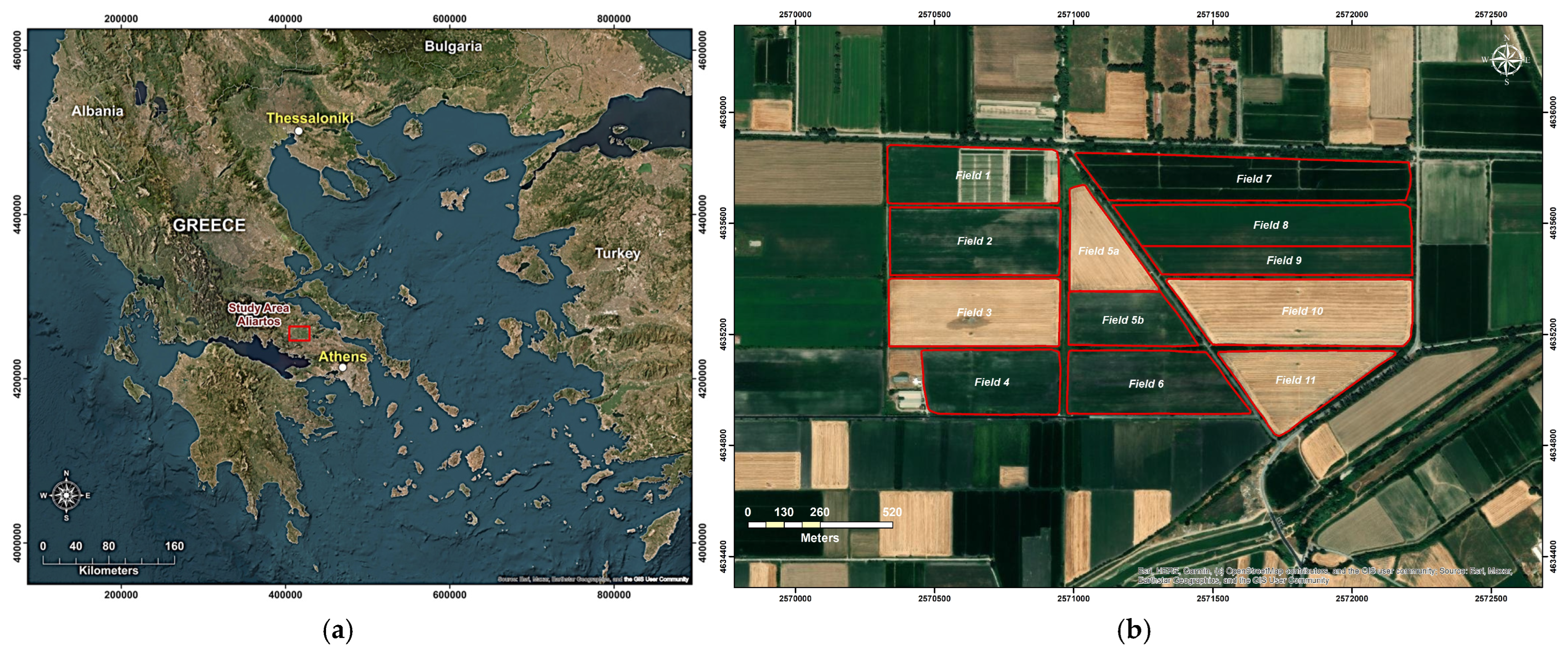
The study was conducted at the experimental agricultural fields of the Agricultural University of Athens, located in Aliartos (38°23′41.64″ N, 23°05′55.60″ E, altitude 105 m a.s.l.), Greece (region of Viotia) (Figure 1). The site lies within the broader Kopaida plain and is characterised by a typical Mediterranean climate, with mild to cool, relatively wet winters and warm to hot, dry summers. These climatic conditions define distinct seasonal environments for crop development and satellite-based observation across the year. The experimental site comprises 12 agricultural fields with individual areas ranging from 4.48 to 11.7 ha. Fields were cultivated with different crops during the study period according to annual crop rotation and experimental design, resulting in variation in the set of fields contributing observations across years and crops. The analysis integrated ten consecutive growing seasons from 2016 to 2025 and included all field–year combinations for which complete yield and Sentinel-2 spectral data were available. Meteorological data used to calculate thermal indices and for climatic contextualisation were obtained from the Kopaida meteorological station operated by the Hellenic National Meteorological Service (EMY). The station is located near the experimental fields and provides representative temperature measurements for the study area. The two crops analysed represent contrasting agronomic systems within the same geographical setting. Wheat was cultivated as a winter cereal, with canopy development occurring primarily during the cooler part of the year, while cotton was cultivated as a summer row crop, developing under warmer seasonal conditions. These differences result in distinct phenological windows and acquisition periods for satellite observations while maintaining a consistent spatial and climatic context.

2.2. Study Design and Analytical Framework

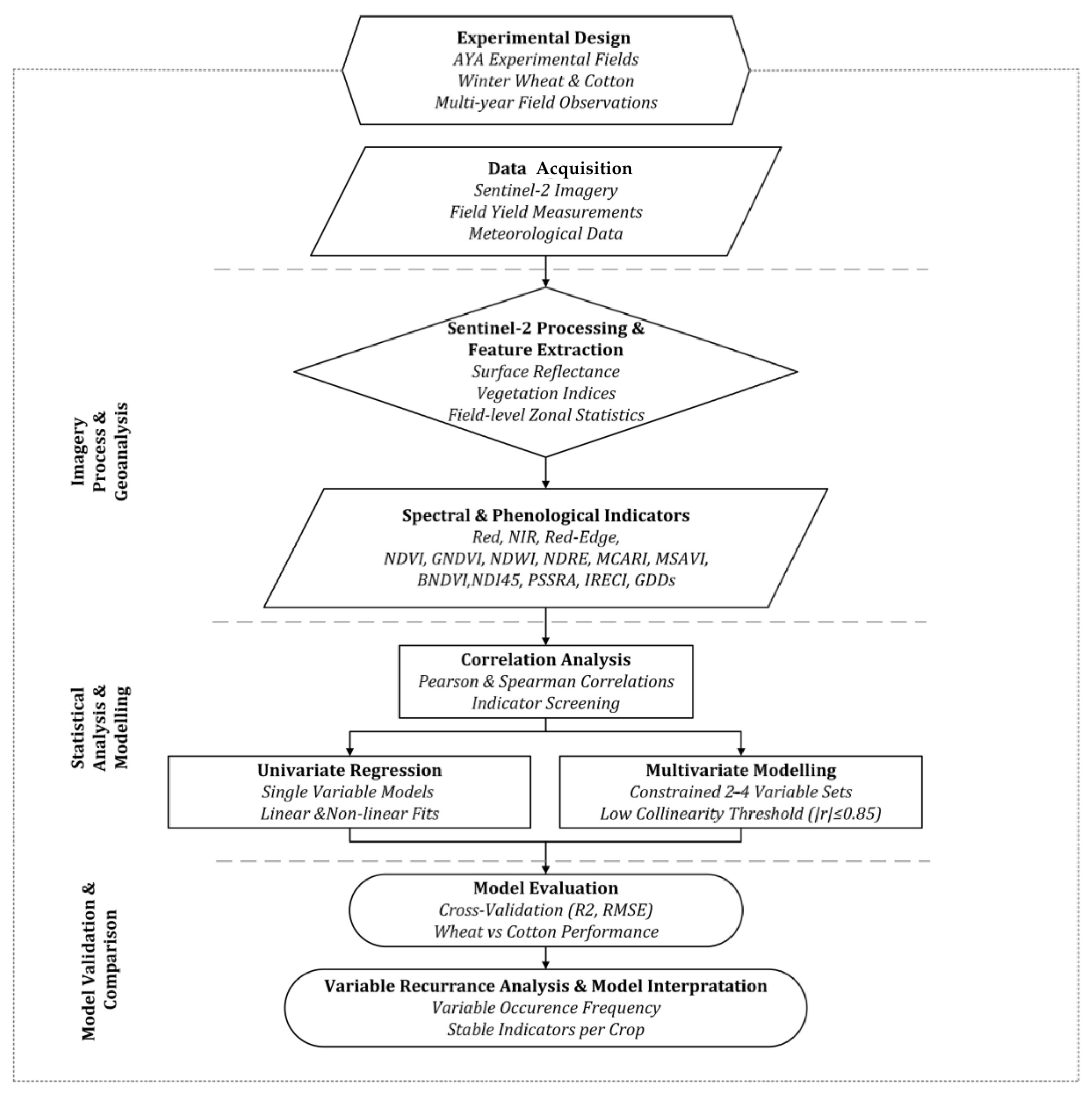
The modelling framework focused exclusively on spectral and phenological indicators. Soil characteristics and management variables (e.g., fertilisation, irrigation, tillage) were not explicitly included in the models. The experimental area is managed using consistent, uniform conventional agronomic practices, with no major management changes throughout the study period. The methodological design of this study follows a stepwise, interpretable analytical framework applied identically to both wheat and cotton to enable direct comparison. The analysis progressively examines yield–spectral relationships through correlation analysis, univariate regression, and constrained multivariate modelling. This structure allows the explicit evaluation of the contributions of individual spectral and phenological indicators before assessing the added value of combining complementary predictors (Figure 2).

All analyses were performed separately for each crop but used the same data structure, feature space, and analytical workflow. Sentinel-2 imagery was processed and pre-processed using ESA SNAP (v. 12.0.0), and all spectral bands and vegetation indices were derived consistently from surface reflectance products following a unified processing chain. Field-level spectral variables were extracted using zonal statistics (e.g., mean reflectance and index values per field polygon) implemented in ArcGIS Pro (v. 3.6.0). The statistical analyses and modelling workflow, including correlation analysis and regression model evaluation, were implemented in a single reproducible modelling environment (Python v. 3.11.9), ensuring that observed differences in yield–spectral relationships could be attributed to crop-specific characteristics rather than methodological inconsistencies. All analyses were executed using standard scientific Python libraries for data handling and modelling. Emphasis was placed on interpretability and agronomic relevance rather than on maximising predictive accuracy through complex black-box approaches, reflecting the study’s limited sample size and the precision agriculture context in which it was applied.

2.3. Dataset Structure and Yield Observations

The analytical dataset was organised at the field–year level, with each record corresponding to one agricultural field monitored during a single growing season. Final measured yield, expressed in kilograms per stremma, was available for all records and served as the dependent variable throughout the analysis.

The study covered ten growing seasons (2016–2025) and included all field–year combinations for which complete yield and spectral data were available. Due to annual crop rotation and experimental planning, not all fields were cultivated with the same crop each year. Consequently, the set of fields contributing observations varied across seasons and crops, resulting in different numbers of field–year entries for wheat and cotton. Consequently, some fields contribute observations in multiple years, depending on crop rotation.

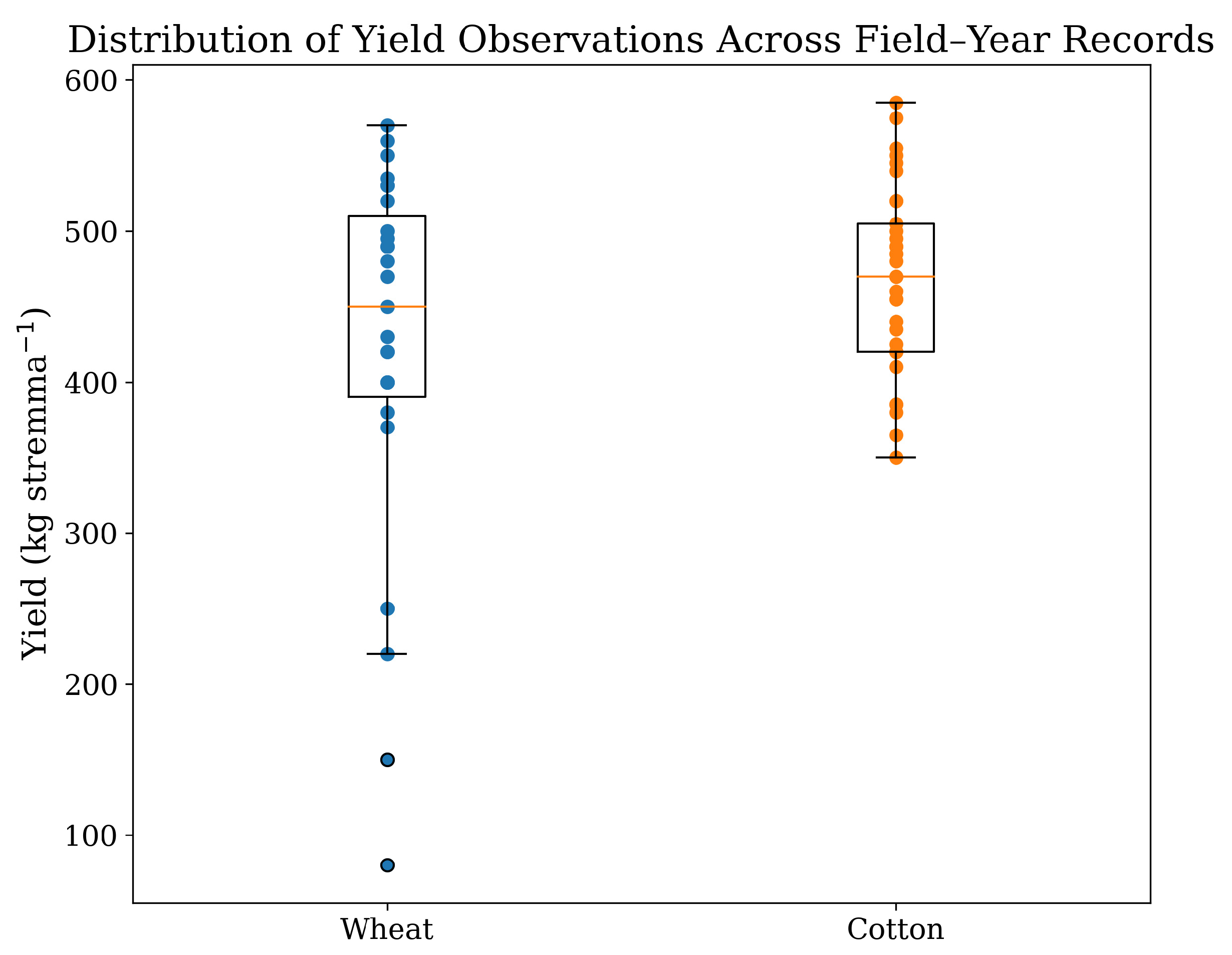
The wheat dataset comprised 27 field–year observations, while the cotton dataset comprised 33. Despite differences in sample size, the two datasets shared the same predictor structure. All spectral, phenological, and derived variables were defined consistently across crops, with differences arising solely from crop-specific satellite image acquisition timing. Across the analysed field–year observations, wheat yields ranged from approximately 80 to 570 kg stremma⁻¹ (mean ± SD: 418 ± 133 kg stremma⁻¹) or 800–5700 kg ha⁻¹ (mean ± SD: 4180 ± 1330 kg ha⁻¹), while cotton yields ranged from approximately 350 to 585 kg stremma⁻¹ (mean ± SD: 468 ± 60 kg stremma⁻¹,) or 3500–5850 kg ha⁻¹ (mean ± SD: 4680 ± 600 kg ha⁻¹ (Figure 3). Yield measurements were obtained directly in the field following harvest operations. For each field–year observation, the entire harvested production from the corresponding field parcel was collected and weighed. This variability reflects interannual climatic variability differences in rainfall distribution, temperature conditions, and seasonal water availability across growing seasons. Additional variability is associated with differences among field parcels and crop rotation conditions within the experimental framework. For consistency and ease of interpretation within the local agronomic context, all analyses were conducted in kg per stremma. These ranges provide context for interpreting the magnitude of reported RMSE values.

A total of 47 predictor variables (excluding identifiers and target variable) were included for each field–year record, comprising raw spectral bands, vegetation indices, phenological variables, and temporal or composite metrics. The complete list of variables and their definitions is provided in

Table 1. Predictor variables used in the analysis, grouped by variable family with corresponding spectral definitions.

Variable Family	Variables	Description	Equation/Spectral Definition
Identification	YEAR, FIELD	Crop season and field identifier	–
Temporal metrics	Ddays	Days between Sentinel-2 acquisitions	Ddays = Date2 − Date1
Thermal metrics	GDD1, GDD2, GDD_DIFF	Thermal accumulation and inter-date progression	GDD = Σ max(0, Tmean − Tbase) [28]; GDD_DIFF = GDD2 − GDD1
Raw spectral bands	RED (1–2), NIR (1–2), RE3(1–2)	Red, near-infrared, and red-edge reflectance	RED = B4 (665 nm); NIR = B8 (842 nm); RE3 = B7 (783 nm)
NDVI family	NDVI (1–2), NDVI_DIFF, NDVI_RATE, NDVI_MEAN, NDVI2_SQ	Canopy greenness and temporal NDVI metrics	NDVI = (NIR − RED)/(NIR + RED) [29]; NDVI_DIFF = NDVI2 − NDVI1; NDVI_RATE = (NDVI2 − NDVI1)/Ddays; NDVI_MEAN = (NDVI1 + NDVI2)/2; NDVI2_SQ = (NDVI2)2
GNDVI family	GNDVI (1–2), GNDVI_DIFF, GNDVI_RATE	Chlorophyll-sensitive greenness indices	GNDVI = (NIR − GREEN)/(NIR + GREEN) [30]
NDWI family	NDWI (1–2), NDWI_DIFF, NDWI_RATE, NDWI_MEAN	Vegetation water status indices	NDWI = (NIR − SWIR)/(NIR + SWIR) [31]; NDWI_DIFF = NDWI2 − NDWI1; NDWI_RATE = (NDWI2 − NDWI1)/Ddays; NDWI_MEAN = (NDWI1 + NDWI2)/2
Red-edge indices	NDRE (1–2), IRECI (1–2)	Red-edge chlorophyll sensitivity	NDRE = (NIR − RE3)/(NIR + RE3) [32]; IRECI = (NIR − RED)/(RE3/RE2) [33]
Pigment indices	MCARI (1–2), PSSRA (1–2)	Chlorophyll and pigment-related indices	MCARI = [(RE3 − RED) − 0.2(RE3 − GREEN)]·(RE3/RED) [34]; PSSRA = NIR/RED [35]
Soil-adjusted indices	MSAVI (1–2), BNDVI (1–2)	Soil background-adjusted vegetation indices	MSAVI = (2·NIR + 1 − √((2·NIR + 1)2 − 8·(NIR − RED)))/2 [36]; BNDVI = (NIR − BLUE)/(NIR + BLUE) [37]
Normalised difference indices	NDI45(1–2)	Green–red contrast indices	NDI45 = (RE − RED)/(RE + RED) [38]
Inter-date band changes	RED_DIFF, RE3_DIFF, NIR_DIFF	Spectral change between acquisitions	Band_DIFF = Band2 − Band1
Composite metrics	NDVI_RATIO, NDVI × NDWI, MCARI × NDRE	Ratio and interaction terms	NDVI_RATIO = NDVI2/NDVI1; NDVI × NDWI = NDVI2·NDWI2; MCARI × NDRE = MCARI2·NDRE2
Target variable	YIELD	Final measured yield	kg stremma−1

Note: Subscripts (1) and (2) denote the first and second Sentinel-2 image acquisitions selected within each growing season, respectively. Variables with subscript 1 correspond to indicators calculated from the earlier acquisition date, while variables with subscript 2 correspond to indicators calculated from the later acquisition date. Inter-date metrics (e.g., _DIFF, _RATE, _MEAN, _RATIO) were derived using values from both acquisitions as specified in the corresponding equations.

. Squared vegetation index terms (e.g., NDVI2_SQ) were included to capture known non-linear and saturating canopy–yield responses, particularly under dense or late-season canopy conditions where linear NDVI sensitivity diminishes (Figure 4).

2.4. Sentinel-2 Data and Spectral Feature Derivation

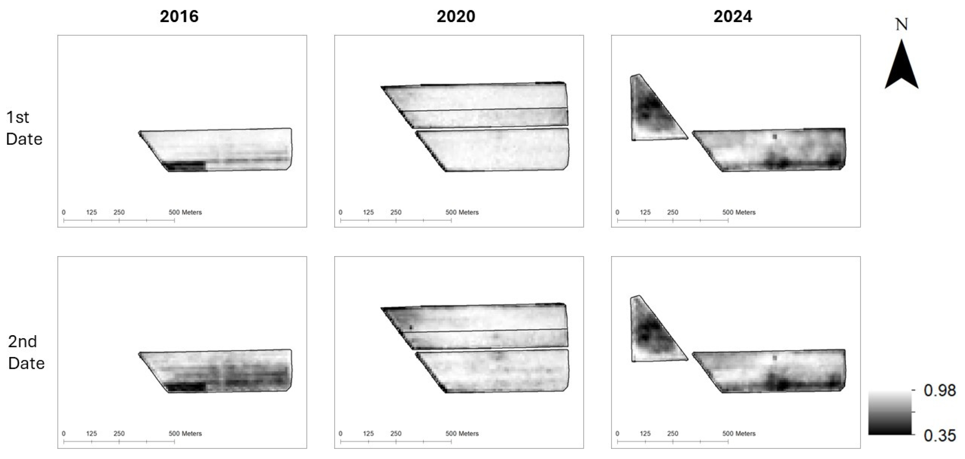
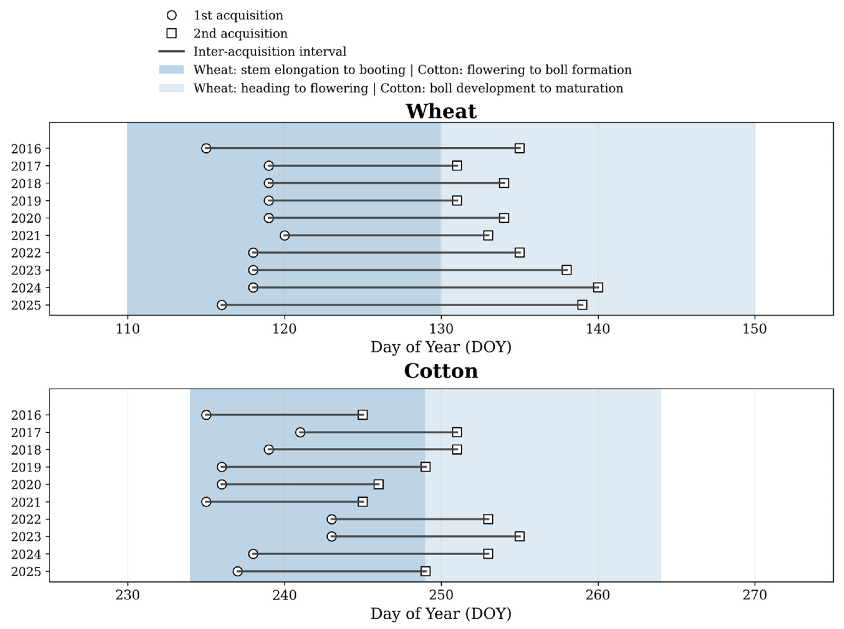
Satellite observations were derived from the Copernicus Sentinel-2 mission, which comprises two identical satellites in the same orbit. Each satellite carries an innovative wide-swath, high-resolution multispectral imager with 13 spectral bands, providing a new perspective on land and vegetation. The Sentinel-2 Level-2A multispectral imagery provides atmospherically corrected surface reflectance data. For each growing season and crop, two cloud-free acquisitions were selected to represent phenologically meaningful stages relevant to yield formation. Acquisition timing was primarily constrained by the availability of cloud-free Sentinel-2 observations during critical crop-development periods, while also aiming to maintain temporal consistency across years. Consequently, the selected dates represent the closest cloud-free acquisitions corresponding to comparable developmental stages among seasons. (Figure 5, Table S1). For wheat, the first acquisition generally corresponded to canopy expansion and stem elongation stages, while the second acquisition corresponded to heading and flowering periods. For cotton, the first acquisition generally corresponded to flowering-to-boll formation stages, whereas the second acquisition corresponded to boll development-to-maturation periods. These acquisition windows are consistent with the typical cropping calendar of the study area, where wheat is typically sown from late December to early January and harvested in early summer, while cotton is established in spring and harvested in late summer to early autumn. Remaining interannual differences in crop development timing were further accounted for through the inclusion of GDD-based and temporal metrics within the analytical framework.

The use of two phenologically representative Sentinel-2 acquisitions per growing season represents a deliberate methodological choice. This design prioritises interpretability and controlled comparison across crops while limiting model complexity given the available sample size. Rather than relying on dense time-series metrics or seasonal integrals, which introduce additional modelling assumptions and data requirements, the selected approach focuses on physiologically meaningful indicators that capture canopy status and change across key developmental stages.

Mean reflectance values were extracted at the field-polygon level and used to compute a comprehensive set of spectral variables. These included raw reflectance bands in the red, near-infrared, and red-edge regions, as well as vegetation indices representing canopy greenness, chlorophyll and pigment sensitivity, vegetation water status, and soil-adjusted canopy structure. To capture intra-seasonal crop dynamics, additional derived metrics were calculated between the two acquisition dates, including inter-date differences, rates of change, ratios, and interaction terms. All spectral variables were computed using standard formulations and aggregated at the field level.

2.5. Phenological and Thermal Variables

Crop phenological development was characterised using Growing Degree Days (GDD) accumulated from the start of each growing season up to each Sentinel-2 acquisition date. Both the accumulated GDD values at each acquisition and the inter-date difference were included to represent thermal progression within the growing season.

These variables were incorporated to provide phenological context to spectral observations and to account for crop-specific sensitivity to thermal accumulation. This representation is particularly relevant for cotton, whose yield formation is strongly influenced by cumulative heat exposure during the growing period.

2.6. Data Pre-Processing and Quality Control

All variables were examined prior to analysis to ensure data integrity and internal consistency. Spectral variables were extracted as field-level means from Sentinel-2 imagery; therefore, no additional spatial aggregation was required. The dataset was screened for missing values and implausible entries, and only complete field–year records were retained for analysis. No data imputation was applied. Variables used solely for identification, such as year and field code, were excluded from all modelling steps.

Predictor variables were retained in their original physical units and index formulations. No explicit standardisation or normalisation was applied, as the analysis prioritised the interpretability of indicator behaviour and included regression model families (e.g., tree-based methods) that are insensitive to variable scaling. Model evaluation relied on cross-validation rather than absolute coefficient magnitudes.

Before multivariate modelling, the correlation structure among predictors was examined as a diagnostic step to assess redundancy and potential multicollinearity among spectral, phenological, and derived variables. Pairwise correlation analysis was used to identify highly correlated variable pairs, informing the constrained predictor selection applied in subsequent multivariate modelling. No automated dimensionality reduction or feature elimination was performed at this stage.

2.7. Correlation Analysis

Correlation analysis was performed using both Pearson’s correlation coefficient and Spearman’s rank correlation coefficient to characterise the relationship between yield and all spectral, phenological, and derived variables. Pearson correlation was used to quantify linear associations, while Spearman correlation was employed to assess monotonic relationships and provide robustness against non-normal distributions and potential outliers.

Correlation matrices were computed separately for wheat and cotton to quantify the strength and direction of yield–indicator relationships, identify crop-specific correlation patterns, and evaluate collinearity among predictors. Correlation heatmaps and ranked correlation tables (Figures S1 and S2) derived from both sets of coefficients were used for exploratory and diagnostic purposes, and to guide the interpretation and selection of variables in subsequent regression analyses. Correlation analysis was used as a comparative and diagnostic tool rather than as a formal hypothesis-testing framework.

2.8. Univariate Regression Analysis

Univariate regression analysis was conducted to quantify the individual explanatory power of each predictor for yield. For each spectral and phenological variable, regression models were fitted independently, without including additional covariates or interaction terms.

Model performance was evaluated using repeated k-fold cross-validation to ensure robustness given the limited sample size. Specifically, a 5-fold cross-validation, repeated three (3) times, was applied; models were trained on 4 folds and evaluated on the remaining fold, with all folds and repetitions iteratively cycled. Cross-validation splits were generated using a fixed random seed to ensure reproducibility across modelling runs. The coefficient of determination (R²) reported for each univariate model corresponds to the mean cross-validated R² across all folds and repetitions.

For each predictor, multiple functional forms were evaluated, including linear and quadratic terms, to capture potential nonlinear or saturating responses. For each variable, the regression method and functional form yielding the highest mean cross-validated R² were retained. This analysis constituted a core step, enabling the identification of dominant individual indicators, the assessment of non-linear behaviour, and the comparison of indicator performance across crops under identical analytical conditions, free from multicollinearity.

2.9. Constrained Multivariate Yield Modelling

Constrained multivariate regression models were developed to assess whether combinations of complementary predictors improved the explanatory power of yield beyond single-indicator models. Multivariate modelling was intentionally restricted to preserve interpretability and to limit overfitting, given the relatively small sample size.

Multivariate models were limited to a small number of predictors (two to four per model). Candidate predictor sets were generated computationally by automatically enumerating all possible predictor combinations within each predictor-size category (k = 2–4). All admissible predictor combinations satisfying the predefined collinearity threshold were evaluated within each predictor-size category. Pairwise correlation filtering was subsequently applied to exclude combinations containing variables exceeding a pairwise Pearson correlation threshold of |r| = 0.85. This relatively conservative threshold was selected to exclude severe redundancy while preserving physiologically related spectral indicators that commonly exhibit moderate correlation in multispectral vegetation-index spaces.

Model performance was evaluated using the same repeated 5-fold cross-validation scheme (three repeats) applied in the univariate analysis, ensuring consistency in performance assessment across modelling stages. Using an identical cross-validation strategy and evaluation metric across the univariate and multivariate stages ensured that model performance comparisons reflected differences in predictor structure rather than differences in the evaluation procedure. Predictor combinations were further guided by univariate performance and by the representation of distinct physiological processes, such as canopy structure, vegetation water status, and phenological development. Separate sets of multivariate models were developed for wheat and cotton using identical selection criteria and modelling logic. The regression model families evaluated at each analytical stage are summarised in

Table 2. List of models used.

Analysis Stage	Model Type	Regression Methods	Predictor Setup
Univariate/Multivariate	Linear	Ordinary Least Squares (OLS), Ridge, Lasso, ARD, Huber	Single predictor/2–4 predictors
	Non-linear	Random Forest, ExtraTrees, AdaBoost, Support Vector Regression (linear and RBF kernels)	Single predictor/2–4 predictors

.

Tree-based ensemble models were implemented using fixed hyperparameter settings across crops and analytical stages to preserve comparability between model configurations. RandomForest and ExtraTrees regressors were implemented using 400 estimators with random_state = 42, while AdaBoost regressors used 400 estimators with a DecisionTreeRegressor base estimator constrained to max_depth = 3 and random_state = 42. Support Vector Regression models were evaluated using both radial basis function (RBF) and linear kernels. Linear, regularised, robust, and Bayesian regression models were implemented using default scikit-learn parameter settings unless otherwise specified.

Cross-validation splits were generated randomly at the field–year level rather than blocked by year or by field. As a result, observations from different years in the same field may appear in both the training and testing folds, potentially introducing partial temporal dependence, particularly for climate-driven predictors such as growing degree days. Consequently, reported performance metrics should be interpreted as upper-bound estimates of explanatory consistency rather than conservative measures of predictive generalisation.

3. Results

3.1. Yield–Spectral Correlation Patterns

Table 3. Strongest correlations between yield and input variables for wheat and cotton.

Crop	Variable	Pearson r	Spearman ρ
Wheat	NDWI_MEAN	0.848	0.715
	NDWI1	0.835	0.707
	MSAVI1	0.819	0.774
	NDWI2	0.804	0.703
	NDVI_MEAN	0.778	0.688
Cotton	GDD_DIFF	−0.588	−0.632
	GDD2	−0.495	−0.433
	RED2	−0.484	−0.535
	NDI452	0.455	0.520
	NDVI2	0.448	0.452

summarises the strongest correlations between yield and selected input variables for wheat and cotton, based on Pearson’s correlation coefficient, together with the corresponding Spearman rank correlations. Among wheat variables, the five with the highest absolute Pearson correlations with yield are NDWI_MEAN, NDWI1, MSAVI1, NDWI2, and NDVI_MEAN. Pearson correlation coefficients for these variables range from 0.778 to 0.848, whereas Spearman correlation coefficients range from 0.688 to 0.774.

For cotton, the five variables with the highest absolute Pearson correlation with yield are GDD_DIFF, GDD2, RED2, NDI452, and NDVI2. Pearson correlation coefficients for these variables range from 0.448 to 0.588 in absolute value, whereas Spearman correlation coefficients range from 0.433 to 0.632. Correlation results are reported separately for each crop and are presented in full in Table 3.

3.2. Univariate Regression Results

Table 4. Best-performing univariate yield models for wheat and cotton.

Crop	Variable	Model	R2	RMSE
Wheat	GDD1	ExtraTrees	0.755	62.27
	GDD1	RandomForest	0.690	70.06
	NDWI_MEAN	OLS	0.672	72.05
	NDWI_MEAN	ARD	0.670	72.26
	NDWI_MEAN	Huber	0.664	72.89
	NDWI_MEAN	Lasso	0.662	73.06
	NDWI1	OLS	0.650	74.40
	NDWI1	ARD	0.649	74.54
	NDWI1	Lasso	0.644	75.02
Cotton	GDD_DIFF	RandomForest	0.439	45.38
	GDD1	RandomForest	0.431	45.73
	GDD_DIFF	AdaBoost	0.430	45.76
	GDD2	RandomForest	0.401	46.92
	GDD1	ExtraTrees	0.391	47.31
	GDD_DIFF	ExtraTrees	0.387	47.45
	GDD2	ExtraTrees	0.376	47.88
	GDD2	AdaBoost	0.365	48.31
	GDD1	AdaBoost	0.356	48.63

presents the highest-performing univariate regression model configurations for wheat and cotton, evaluated using the coefficient of determination (R²). Multiple regression methods were tested for each predictor, and Table 4 reports the top-performing variable–model combinations based on R².

For wheat, the highest univariate performance was obtained using GDD1 with an ExtraTrees regressor (R² = 0.755). Additional high-performing wheat models include a Random Forest regression using GDD1 (R² = 0.690), as well as several linear model configurations based on NDWI-derived variables. Specifically, OLS, ARD, Huber, and Lasso regressions applied to NDWI_MEAN achieved R² values ranging from 0.662 to 0.672, whereas NDWI1-based linear models achieved R² values ranging from 0.644 to 0.650.

For cotton, the strongest univariate models were dominated by thermal variables. The highest R² values were obtained using RandomForest regressors with GDD_DIFF (R² = 0.439), GDD1 (R² = 0.431), and GDD2 (R² = 0.401). Additional univariate models using ExtraTrees and AdaBoost regressors applied to GDD-based variables also exhibited comparatively strong performance, with R² values ranging from 0.356 to 0.391. Corresponding root mean square error (RMSE) values for all listed models are provided alongside R² and are expressed in kilograms per stremma (kg stremma⁻¹).

3.3. Constrained Multivariate Modelling Results

Table 5. Top 10 constrained multivariate yield models for wheat, ranked by mean cross-validated coefficient of determination (R²). Corresponding root mean square error (RMSE) values are expressed in kg stremma⁻¹.

k	Predictors	Model	R2	RMSE
4	GDD1 + NDWI_DIFF + NIR_DIFF + IRECI1	ExtraTrees	0.701	54.418
4	GDD2 + NDVI_RATE + NDWI2 + RE3_DIFF	ExtraTrees	0.692	52.352
4	Ddays + GDD2 + NDWI_DIFF + PSSRA2	ExtraTrees	0.687	55.016
4	GDD2 + NDWI_DIFF + RE3_DIFF + PSSRA2	ExtraTrees	0.675	53.372
4	Ddays + NDWI2 + NIR_DIFF + PSSRA1	Lasso	0.670	50.966
4	Ddays + NDWI2 + NIR_DIFF + PSSRA1	OLS	0.670	48.017
3	Ddays + NDWI2 + NIR_DIFF	Huber	0.668	48.747
4	GDD1 + GNDVI_RATE + RED_DIFF + MSAVI1	OLS	0.663	55.168
4	Ddays + GDD_DIFF + GNDVI1 + RED_DIFF	ExtraTrees	0.657	54.189
4	Ddays + GDD_DIFF + GNDVI1 + RE3_DIFF	ExtraTrees	0.655	52.665

and

Table 6. Top 10 constrained multivariate yield models for cotton, ranked by mean cross-validated coefficient of determination (R²). Corresponding root mean square error (RMSE) values are expressed in kg stremma⁻¹.

k	Predictors	Model	R2	RMSE
3	GDD_DIFF + NDVI_MEAN + NDWI_RATE	ExtraTrees	0.741	27.673
2	GDD_DIFF + NDVI_MEAN	ExtraTrees	0.732	26.687
3	GDD_DIFF + NDWI_RATE + NDVI × NDWI	ExtraTrees	0.725	28.903
4	Ddays + GDD_DIFF + NDVI_MEAN + NIR2	ExtraTrees	0.722	27.763
4	GDD1 + NDVI2_SQ + RE3_1 + RE3_DIFF	ExtraTrees	0.719	27.108
3	GDD1 + NDVI2_SQ + MCARI2 × NDRE2	ExtraTrees	0.716	28.621
4	GDD_DIFF + NDI452 + BNDVI1 + MSAVI1	ExtraTrees	0.714	28.061
4	GDD1 + NDVI2_SQ + NDWI1 + MCARI1	ExtraTrees	0.714	28.261
4	GDD1 + RED2 + NIR_DIFF + MCARI1	ExtraTrees	0.714	28.735
4	GDD1 + NDVI1 + NDVI2 + MCARI1	ExtraTrees	0.714	27.734

summarise the highest-performing constrained multivariate models for wheat and cotton, respectively. For wheat, multivariate models included between three and four predictors and achieved mean cross-validated R² values ranging from 0.701 to 0.655. The top-performing wheat model combined GDD1, NDWI_DIFF, NIR_DIFF, and IRECI1 using an ExtraTrees regression, achieving a mean cross-validated R² of 0.701 and an RMSE of 54.418 kg stremma⁻¹ (544.18 kg ha⁻¹). Across the highest-ranked wheat models, vegetation water-status indicators (NDWI_DIFF, NDWI2), and inter-date canopy-dynamics metrics (NIR_DIFF, RE3_DIFF), thermal accumulation variables (GDD1, GDD2, GDD_DIFF), temporal metrics (Ddays) and pigment-related indices (PSSRA1, PSSRA2) appeared recurrently within top-performing predictor combinations. Multiple regression families, including ExtraTrees, OLS, Lasso, and Huber estimators, achieved comparable performance under the constrained-predictor framework. Additional high-performing wheat models and their corresponding RMSE values are reported in Table 5.

For cotton, constrained multivariate models included between two and four predictors and achieved mean cross-validated R² values ranging from 0.741 to 0.714. The top-performing cotton model combined GDD_DIFF, NDVI_MEAN, and NDWI_RATE using an ExtraTrees regression, achieving a mean cross-validated R² of 0.741 and an RMSE of 27.673 kg stremma⁻¹ (276.73 kg ha⁻¹). Additional high-performing cotton models included combinations of thermal accumulation metrics (GDD1, GDD_DIFF), temporal metrics (Ddays), canopy-greenness indicators (NDVI_MEAN, NDVI2_SQ, BNDVI1), vegetation-water-status indicators (NDWI1, NDWI_RATE), inter-date spectral-change variables (NIR_DIFF, RE3_DIFF), and pigment-related indices (MCARI1, MCARI2 × NDRE2). All reported high-performing cotton models were obtained using ExtraTrees regressors. Additional high-performing cotton models and their corresponding RMSE values are reported in Table 6.

Following pairwise correlation filtering (|r| ≤ 0.85), the constrained multivariate workflow evaluated 812 admissible two-predictor combinations, 9011 admissible three-predictor combinations, and 66,206 admissible four-predictor combinations across the examined predictor space. The recurrence analysis presented in Section 3.4 was subsequently derived from the top 100 models ranked according to mean cross-validated R² values.

3.4. Variable Recurrence Across Constrained Multivariate Models

Table 7. Frequency of variable occurrence (n) in the top 100 constrained multivariate models.

Wheat		Cotton
Variable	Occurrences (n)	Variable	Occurrences (n)
GNDVI_DIFF	1	RED2	1
NIR2	1	MSAVI2	1
NDVI_DIFF	1	BNDVI2	1
NDVI2	1	NDVI_RATIO	1
MSAVI1	2	GNDVI_RATE	1
NDWI1	2	Ddays	2
NDI451	2	IRECI1	2
NDVI1	2	PSSRA1	2
RE3_2	2	RED_DIFF	2
BNDVI1	2	NDVI_RATE	2
IRECI2	2	MCARI2	2
IRECI1	3	GNDVI2	2
RED2	3	NDWI_DIFF	3
MCARI2	3	NIR_DIFF	4
GNDVI1	4	RE3_DIFF	5
RED1	4	NDI451	5
NIR1	5	MCARI2 × NDRE2	6
GNDVI_RATE	6	MSAVI1	6
NDVI_RATIO	6	NDWI1	6
NDI452	6	NIR1	6
GDD1	7	GNDVI1	6
NDVI_RATE	7	RE3_1	7
RE3_1	8	BNDVI1	7
NDVI × NDWI	8	NDWI_MEAN	7
RED_DIFF	9	NDWI_RATE	8
NDWI_RATE	9	NDVI × NDWI	8
PSSRA1	10	MCARI1	8
GDD_DIFF	10	IRECI2	8
PSSRA2	12	NDVI1	9
NDWI_MEAN	16	RED1	9
NDWI_DIFF	17	NIR2	10
Ddays	29	NDI452	11
RE3_DIFF	31	NDWI2	11
GDD2	33	GDD2	14
NDWI2	38	NDVI2	17
NIR_DIFF	40	NDVI2_SQ	19
		NDVI_MEAN	24
		GDD1	40
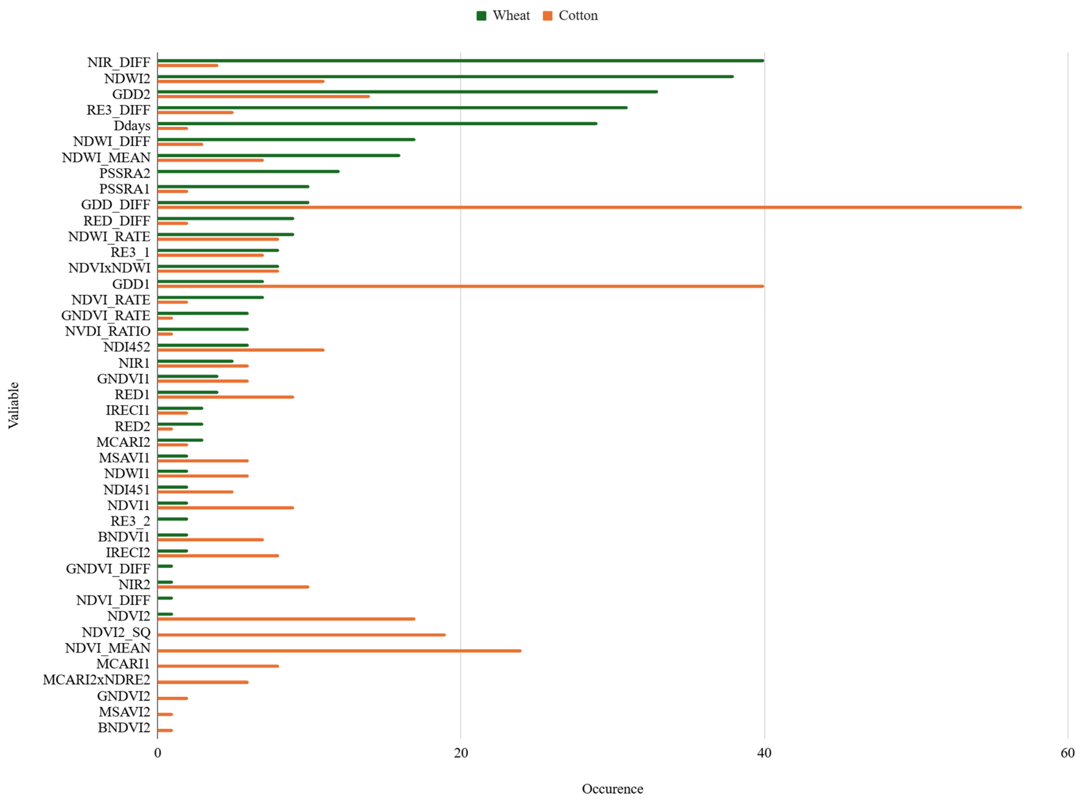
		GDD_DIFF	57

summarises the frequency with which individual variables appear across the top 100 constrained multivariate models for wheat and cotton. Frequencies are reported separately for each crop and represent the number of occurrences of each variable across the selected model set. The top 100 models were ranked according to mean cross-validated R² values obtained under the constrained multivariate modelling framework. Recurrence frequency is reported as a descriptive indicator of stability within the constrained model space and does not imply statistical importance, causal dominance, or independent explanatory power.

For wheat, the highest recurrence is observed for NIR_DIFF, which appears in 40 of the top 100 models, followed by NDWI2 (38 occurrences), GDD2 (33 occurrences) and RE3_DIFF (31 occurrences). Additional variables with notable recurrence include Ddays, NDWI_DIFF, NDWI_MEAN, and PSSRA2, each appearing in more than ten models. A broader set of variables appears less frequently, with multiple predictors occurring fewer than five times across the model set. For cotton, the most frequently occurring variable across the top 100 models is GDD_DIFF, with 57 occurrences, followed by GDD1 (40 occurrences) and NDVI_MEAN (24 occurrences). Several vegetation indices and interaction terms, including NDVI2_SQ, NDVI2, GDD2, NDWI2, NDI452, and NIR2, also appear repeatedly across the model set, with occurrence counts ranging from 10 to 19. Additional variables exhibited lower recurrence frequencies across the constrained model space.

Across both crops, Table 7 and Figure 6 report the full distribution of variable recurrence within the constrained multivariate model space. No ranking or weighting beyond raw frequency is applied, and all counts reflect model inclusion only.

4. Discussion

4.1. Crop-Specific Yield Drivers Under a Unified Sentinel-2 Indicator Framework

Under a fully unified Sentinel-2 indicator framework, yield–spectral relationships exhibit clearly distinct, crop-specific patterns, even when observational and analytical conditions are held constant [8]. Crop yield integrates multiple physiological processes whose relative importance varies across crop types, phenological cycles, and environmental conditions, a pattern consistently reported in both agronomic and satellite-based yield studies [39]. By analysing two contrasting crops under identical observational and analytical conditions within a unified indicator framework, this study enables clearer identification of crop-specific physiological drivers of yield variability with minimal methodological interference, which is often a limiting factor in multi-crop yield estimation studies due to differences in acquisition timing, feature selection, and modelling strategy [40,41]. Within this controlled framework, wheat yield variability was most strongly associated with water-sensitive, canopy-structure-related, and inter-date canopy-dynamics indicators, whereas cotton yield variability was more strongly associated with thermal accumulation metrics and complementary spectral indicators related to canopy condition and vegetation status.

These findings are consistent with a broad body of literature describing wheat yield formation as highly sensitive to seasonal water availability, canopy development, and moisture stress during critical growth stages, particularly under Mediterranean and semi-arid conditions [16,26,42]. The prominence of NDWI-derived variables and soil- and canopy-adjusted greenness indices reflects the direct roles of vegetation water status and canopy structure in regulating biomass accumulation and grain filling. NDWI is explicitly designed to capture variations in vegetation water content and canopy moisture [31], and its relevance for diagnosing crop water stress and productivity limitations has been demonstrated in both field-based and satellite-driven studies [43]. The recurrent appearance of red-edge and near-infrared inter-date change metrics further aligns with studies demonstrating that these spectral regions are particularly sensitive to chlorophyll dynamics and canopy structural variation closely linked to yield formation in cereals [6,38].

In contrast, cotton yield variability showed a strong association with thermal accumulation indicators, consistent with agronomic evidence that cotton development, flowering, and boll retention are strongly regulated by cumulative heat exposure and temperature-driven phenological progression [44,45,46,47]. The strong recurrence of growing degree-day (GDD) variables across analytical stages is consistent with findings from both field-based and remote-sensing studies that identify thermal time as a primary control on cotton yield potential and yield losses under heat-stress conditions [46,48]. The co-occurrence of selected spectral indicators, including NDVI- and pigment-sensitive metrics, suggests that canopy condition provides complementary explanatory information once phenological timing and thermal exposure are accounted for, as reported in recent cotton monitoring and yield estimation studies using optical remote sensing [27,48,49]. In contrast to wheat, these patterns highlight the shift from predominantly water-sensitive and canopy-related yield controls toward stronger temperature-driven phenological regulation across seasonal cropping systems.

Overall, these results demonstrate that, when methodological variability is minimised, crop physiology appears to represent a major source of variation in yield–spectral relationships under the controlled analytical conditions examined in this study. These findings reinforce the importance of selecting crop-specific indicators and support the use of physiologically grounded, interpretable feature sets in remote sensing applications for precision agriculture.

4.2. Consistency of Indicator Behaviour Across Analytical Stages

Throughout the following analysis, individual model rankings are not interpreted deterministically. Given the small sample size and the presence of correlated predictors, multiple near-equivalent model configurations are expected. Consequently, interpretation focuses on recurrent indicator families and their physiological relevance across analytical stages rather than on any single ‘best-performing’ model.

A central contribution of this study is the explicit examination of indicator behaviour across multiple analytical stages, including correlation analysis, univariate regression, constrained multivariate modelling, and frequency-based recurrence within the top model set. Many yield-estimation studies prioritise reporting a single optimised model, often focusing on predictive accuracy, while providing limited insight into whether identified predictors represent stable yield drivers or artefacts of a particular modelling configuration [23,41]. Such approaches can obscure the agronomic relevance of individual indicators, particularly when complex or high-dimensional models are applied to relatively small datasets. By contrast, the present results indicate that certain indicator families exhibit consistent recurrence across analytical stages, while others exhibit stage-specific or context-dependent relevance.

For wheat, NDWI-based indicators consistently rank among the strongest predictors in correlation, univariate, and multivariate analyses and exhibit high recurrence within the constrained model space. This multi-stage consistency supports the interpretation that vegetation water status represents a recurrently associated and physiologically interpretable indicator family under the study conditions, in agreement with studies emphasising the role of soil moisture availability and evaporative demand in regulating cereal productivity, biomass accumulation, and grain filling [26,50]. For cotton, the repeated recurrence of GDD-based predictors across analytical stages is consistent with agronomic evidence that temperature-driven development and cumulative heat exposure are closely associated with yield variability across seasons [42,44,48]. The persistence of these indicator families across analytical stages strengthens confidence that they represent recurrently associated indicator families rather than isolated model-dependent effects.

Despite variability in field parcels and growing seasons, several indicators were consistently observed across models, suggesting that remote sensing signals can capture recurrent patterns in crop performance under heterogeneous field conditions. This consistency further supports the physiological interpretability of the identified indicator families and highlights their potential relevance for operational applications in precision agriculture, where variability in field conditions is inherent. The exceptionally high univariate performance observed for selected tree-based models should nevertheless be interpreted cautiously, given the limited sample size and the known sensitivity of flexible ensemble methods to small datasets. The recurrence and consistency of indicator families across analytical stages were therefore considered more informative than isolated top-performing model scores.

4.3. Reconciling Correlation Strength with Multivariate Recurrence

An important finding of this study is that variables exhibiting the strongest correlation with yield are not always those that dominate recurrence within the constrained multivariate model space. While correlation-based screening remains a widely used initial step in yield modelling, it primarily captures linear or monotonic associations and may not fully reflect the contribution of predictors within multivariate, physiologically structured relationships. Recent work in remote sensing–based yield modelling and explainable feature analysis has highlighted that correlation-based rankings can overlook variables whose explanatory contribution emerges primarily through complementary or conditional effects when combined with other predictors [51,52]. As a result, reliance on correlation strength alone may underestimate the agronomic relevance of indicators that contribute to yield variability through interaction with distinct physiological processes. Strong correlation does not necessarily imply the maximum explanatory contribution in multivariate settings, particularly when key drivers, such as thermal accumulation and water status, capture distinct, partially orthogonal dimensions of crop response.

In wheat, although NDWI_MEAN and NDWI1 exhibit strong correlation with yield, recurrence analysis highlights NDWI2, RE3_DIFF, and NIR_DIFF as more frequent components of multivariate model configurations. This pattern suggests that phenologically targeted indicators, particularly those capturing later-stage canopy water status and inter-date canopy dynamics, may contribute complementary explanatory information when combined with additional predictors relative to static or season-averaged metrics alone. Similar findings have been reported in studies emphasising the importance of growth-stage-specific indicators and intra-seasonal canopy dynamics for yield explanation, particularly under water-limited conditions where the timing of stress, rather than its seasonal average, governs yield outcomes [3,25].

In cotton, thermal accumulation indicators remain highly recurrent across both correlation ranking and recurrence analysis, indicating that thermal accumulation was consistently associated with yield variability under the examined conditions. This persistence suggests that temperature-driven phenological progression represents an important component of yield variability, while spectral indicators provide complementary information on canopy condition within this thermal framework. Recent cotton-focused studies similarly report that cumulative heat exposure is closely associated with key developmental processes, while spectral indicators capture complementary responses related to canopy condition and temperature-driven growth dynamics [48].

Overall, these results highlight that multivariate recurrence provides a complementary perspective to correlation-based analysis, enabling the identification of recurrently associated and physiologically interpretable predictors that may not be apparent from correlation strength alone. This reinforces the importance of moving beyond single-metric ranking approaches toward integrated, multi-stage evaluation frameworks when interpreting yield–spectral relationships.

4.4. Implications for Indicator Selection and Agronomic Interpretability

The results reinforce the broader argument that yield estimation from remote sensing is not solely a modelling problem, but fundamentally an indicator interpretation and physiological attribution problem. A recurring limitation in recent yield-modelling literature is the emphasis on maximising predictive accuracy through large, high-dimensional feature sets and complex model architectures, often with limited physiological justification and reduced transparency [19,23,46,51]. While such approaches can achieve high predictive performance, they are frequently difficult to translate into actionable agronomic insight, particularly in precision agriculture contexts where decision relevance, trust, and operational interpretability are critical [18,23,51].

The present findings support a more parsimonious and physiologically grounded strategy for indicator selection. Across both crops, a limited set of carefully selected indicators was consistently associated with a substantial proportion of observed yield variability under the examined conditions, demonstrating that simple, interpretable models provide meaningful explanatory capability for field-level crop monitoring. This result highlights that model complexity is not a prerequisite for achieving meaningful explanatory performance, particularly when predictors align with key physiological processes, such as vegetation water status and thermal accumulation.

For wheat, prioritising indicators related to vegetation water status and canopy structural dynamics aligns with operational monitoring practices focused on drought stress detection, canopy development, and biomass accumulation, which are increasingly adopted in satellite-based decision-support systems for cereal production [3,11,26]. For cotton, combining thermal accumulation metrics with complementary canopy spectral indicators reflects established and modern agronomic approaches that integrate phenological tracking with canopy condition to contextualise yield outcomes and management decisions [48].

Importantly, the use of constrained multivariate combinations demonstrates that improved yield explanation can be achieved without resorting to high-dimensional or opaque modelling approaches. This finding supports the development of transparent, interpretable, and crop-aware modelling strategies that are better aligned with the practical requirements of precision agriculture. In operational contexts, where data availability, computational resources, and user interpretability are often limiting factors, such parsimonious approaches provide a more operationally accessible and interpretable alternative to complex modelling frameworks [19,51].

4.5. Value of Controlled Cross-Crop Comparison Under Identical Data Structure

Cross-crop comparisons in yield modelling are often difficult to interpret because existing studies frequently differ in acquisition timing, predictor definitions, spatial aggregation, and modelling strategies across crops, making it challenging to disentangle crop physiology from methodological effects [15,26,41,53]. As a result, reported differences in yield–spectral relationships across crops are often confounded by variations in analytical design rather than reflecting genuine biological contrasts.

By holding the feature space, data structure, and analytical workflow consistent across crops, this study enables clearer comparison of crop-specific yield–spectral relationships under controlled observational and analytical conditions. The observed differences in recurrently associated indicator families are therefore less likely to reflect methodological inconsistencies related to acquisition timing, predictor structure, or modelling strategy. This controlled comparison strengthens the interpretability of crop-specific findings and highlights the importance of analysing yield–spectral relationships under consistent methodological assumptions when comparing contrasting crop systems. Similar needs for unified and crop-comparable analytical frameworks have been emphasised in recent multi-crop and large-scale yield-monitoring studies, particularly in the context of operational remote sensing applications [51,54].

As such, the framework presented here provides a structured comparative approach for evaluating crop-specific yield–spectral relationships under controlled analytical conditions. Future studies applying similar unified workflows across additional crops, sites, and environmental conditions may further support interpretation of the extent to which recurrent indicator behaviour reflects crop physiology, seasonal context, or observational design [3,15].

4.6. Limitations and Future Research

Several limitations should be considered when interpreting the results of this study. First, the number of field–year observations is relatively limited, which constrains the complexity of multivariate models and restricts the exploration of higher-order interactions. Although repeated cross-validation was applied to support comparative model evaluation, the identified indicator rankings and recurrence patterns remain conditioned by the available sample size and site-specific context. This limitation is common in field-scale and experimental yield studies based on satellite observations, where data availability is often constrained by monitoring logistics and experimental design [19,41].

Second, the analysis relies on two Sentinel-2 acquisitions per growing season. While this design supports interpretability and phenological targeting, it may not capture short-term stress events, transient water deficits, or rapid canopy changes that influence yield formation, particularly under variable weather conditions [3]. Future work could evaluate whether higher-temporal-resolution time series metrics, such as seasonal integrals, peak timing, or curve-shape descriptors derived from dense satellite observations, improve indicator stability and explanatory power without compromising interpretability [25].

Third, the modelling framework focuses exclusively on spectral and phenological indicators, without explicitly incorporating soil properties, management practices, or detailed weather variability beyond thermal accumulation. While this design was intentional to isolate the contribution of remote-sensing-derived indicators under controlled conditions, it limits the ability to disentangle environmental- and management-driven effects on yield variability. Integrating spectral data with soil, climate, and management variables represents a key direction for future work and may enhance both explanatory robustness and operational relevance in precision agriculture applications [15,19].

Finally, the cross-validation strategy was applied at the field–year level without explicitly accounting for temporal or spatial dependence. As a result, observations from different years within the same field may appear in both the training and testing folds, potentially leading to optimistic performance estimates. Future studies could implement stricter validation schemes, such as leave-one-year-out or field-blocked cross-validation, to further assess the generalisation capacity of the identified indicator relationships under more independent conditions.

Despite these limitations, the study provides a controlled and interpretable framework for analysing yield–spectral relationships, enabling the identification of recurrently associated and physiologically interpretable indicator families across crops. Future research building on this approach can extend its applicability by incorporating additional data sources, increasing temporal resolution, and evaluating robustness across broader agroecological contexts.

5. Conclusions

Under a fully unified Sentinel-2 indicator framework applied consistently across wheat and cotton, this study demonstrates that yield–spectral relationships are strongly crop-dependent when examined under identical observational and analytical conditions. By controlling methodological variability, the analysis supports the interpretation that crop physiology represents a major source of variation in indicator behaviour under the examined conditions.

Wheat yield variability was most consistently associated with water-sensitive and canopy-related indicators, reflecting the importance of vegetation water status and structural development during critical growth stages. In contrast, cotton yield variability showed a stronger association with thermal accumulation metrics together with complementary spectral indicators, highlighting the central role of temperature-driven phenological progression in warm-season crop yield formation. These contrasting indicator patterns can be explained by fundamental differences in crop physiology, phenology, and water demand between winter cereals and summer crops. Wheat, cultivated as a winter cereal under Mediterranean conditions, develops during cooler, wetter periods, when water availability and canopy dynamics play an important role, whereas cotton develops under warmer conditions, where cumulative heat exposure represents an important component of phenological development and yield variability.

Importantly, these crop-specific indicator families showed recurrent behaviour across multiple analytical stages, including correlation analysis, univariate regression, and constrained multivariate modelling. Their repeated occurrence across top-performing model configurations indicates that they represent recurrently associated and physiologically interpretable indicator families under the examined conditions, rather than artefacts of a particular modelling approach. Despite variability in field parcels and growing seasons, a limited set of indicators was consistently associated with a substantial proportion of observed yield variability under the examined conditions, demonstrating that parsimonious and interpretable models may provide meaningful explanatory capability for field-level crop monitoring.

More broadly, the results highlight that yield estimation from remote sensing should not be viewed solely as a modelling problem, but fundamentally an issue of indicator selection and physiological interpretation. The findings support the use of crop-aware, physiologically grounded indicator frameworks and demonstrate that simple, well-targeted predictor sets can provide meaningful explanatory capability without reliance on complex or opaque modelling approaches.

The unified analytical framework presented in this study offers a structured comparative approach for evaluating crop-specific yield–spectral relationships across contrasting crop systems, enabling clearer separation of biological signal from methodological artefacts. This is particularly relevant for operational precision agriculture applications, where interpretable and operationally accessible methods are increasingly required to support multi-crop monitoring under heterogeneous field conditions.