Author Contributions
Conceptualization, H.L., X.D. and T.P.; methodology, H.L., Y.L., X.C. and Y.Y. (Yongqi Yin); software, H.L., Y.L., Q.H., Y.Y. (Yujie Yao) and X.C.; validation, H.L., Y.L., Q.H., B.L. and Y.Y. (Yujie Yao); formal analysis, H.L., Y.L., Q.H., Y.X., X.D. and T.P.; investigation, H.L., B.L., W.W., H.H., Y.X. and X.C.; resources, H.H., Y.Y. (Yongqi Yin), X.D. and T.P.; data curation, Q.H., B.L., W.W., H.H., Y.X. and Y.Y. (Yujie Yao); writing—original draft preparation, H.L., Y.L. and Q.H.; writing—review and editing, Y.L., Y.Y. (Yongqi Yin), X.D. and T.P.; visualization, H.L. and W.W.; supervision, X.D. and T.P.; project administration, X.D. and T.P. All authors have read and agreed to the published version of the manuscript.
Figure 1.
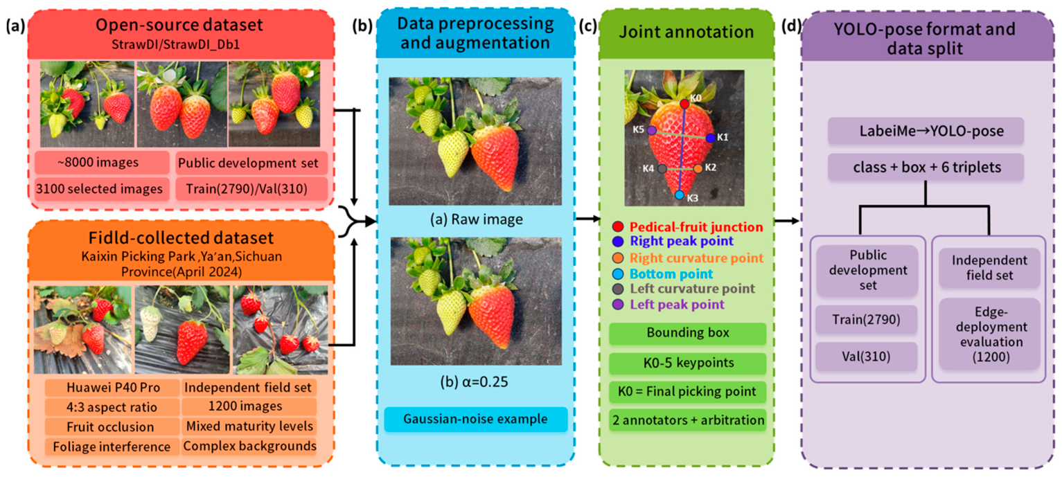
Pipeline for constructing the strawberry picking point dataset. (a) Image sources, including the public StrawDI-derived development set and the independent field-collected set. (b) Preprocessing and online data augmentation used during model training. (c) Joint annotation of strawberry bounding boxes and six keypoints. (d) Dataset usage, including training, validation, and deployment-oriented evaluation.
Figure 1.
Pipeline for constructing the strawberry picking point dataset. (a) Image sources, including the public StrawDI-derived development set and the independent field-collected set. (b) Preprocessing and online data augmentation used during model training. (c) Joint annotation of strawberry bounding boxes and six keypoints. (d) Dataset usage, including training, validation, and deployment-oriented evaluation.
Figure 2.
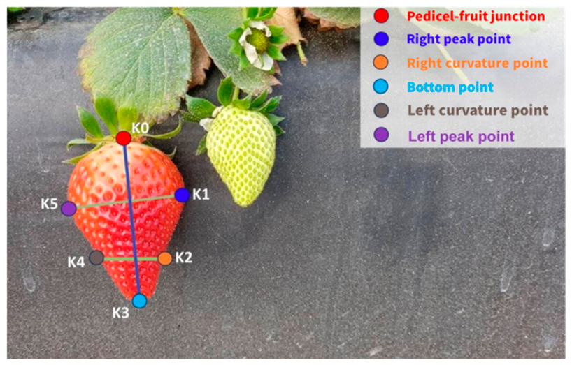
Six-keypoint annotation scheme for strawberry picking point modeling.
Figure 2.
Six-keypoint annotation scheme for strawberry picking point modeling.
Figure 3.
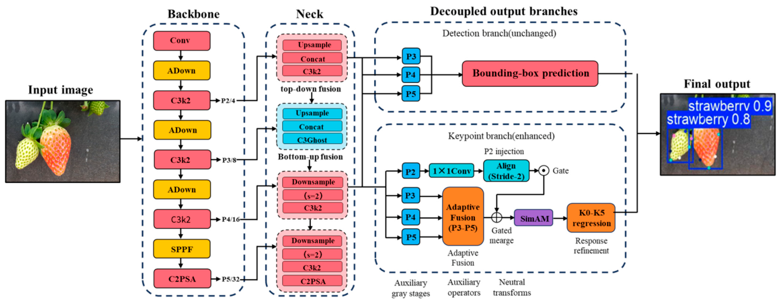
Overall architecture of the proposed StrawPose-Lite model. The main modified components are ADown in the backbone, C3Ghost in the neck, and the keypoint branch enhancement module in the keypoint branch. The keypoint branch enhancement module consists of P3–P5 adaptive fusion, gated P2 feature injection, and SimAM refinement.
Figure 3.
Overall architecture of the proposed StrawPose-Lite model. The main modified components are ADown in the backbone, C3Ghost in the neck, and the keypoint branch enhancement module in the keypoint branch. The keypoint branch enhancement module consists of P3–P5 adaptive fusion, gated P2 feature injection, and SimAM refinement.
Figure 4.
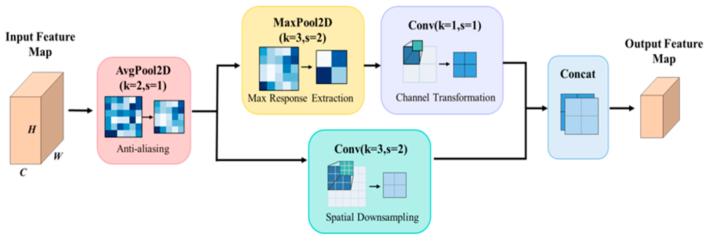
Structure of the ADown anti-aliasing downsampling module.
Figure 4.
Structure of the ADown anti-aliasing downsampling module.
Figure 5.
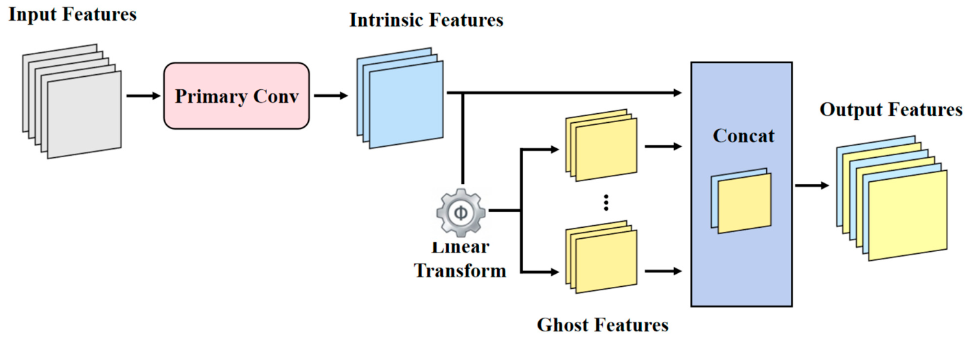
Structure of the C3Ghost lightweight feature extraction module.
Figure 5.
Structure of the C3Ghost lightweight feature extraction module.
Figure 6.
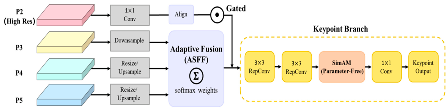
P3-oriented adaptive multi-scale fusion in the keypoint branch. Projected P3–P5 features are aligned to a common resolution, fused by learnable softmax weights, and refined by a zero-initialized spatial correction path before high-resolution P2 injection.
Figure 6.
P3-oriented adaptive multi-scale fusion in the keypoint branch. Projected P3–P5 features are aligned to a common resolution, fused by learnable softmax weights, and refined by a zero-initialized spatial correction path before high-resolution P2 injection.
Figure 7.
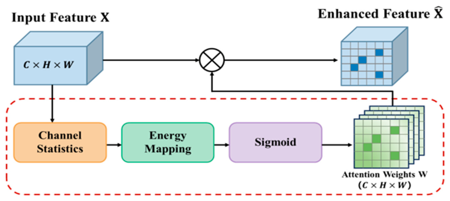
Structure of the SimAM refinement path used in the keypoint branch. SimAM is inserted after the RepConv refinement stack and before the final output layer so that fine pedicel-related responses can be recalibrated without extra learnable parameters.
Figure 7.
Structure of the SimAM refinement path used in the keypoint branch. SimAM is inserted after the RepConv refinement stack and before the final output layer so that fine pedicel-related responses can be recalibrated without extra learnable parameters.
Figure 8.
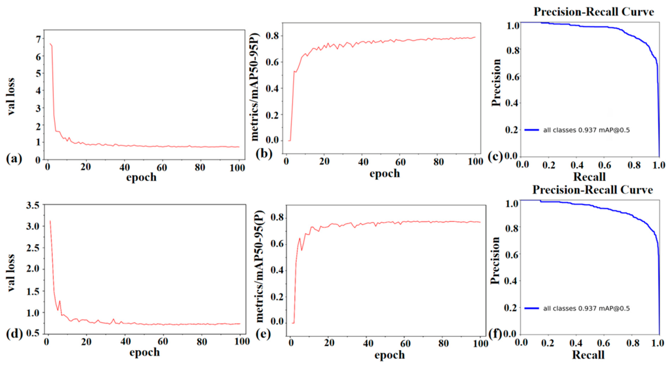
Training convergence and validation performance comparison between StrawPose-Lite and the YOLOv11n-pose baseline under the public validation split. (a) Validation loss of StrawPose-Lite; (b) pose mAP@0.5:0.95 of StrawPose-Lite; (c) precision–recall curve of StrawPose-Lite; (d) validation loss of YOLOv11n-pose baseline; (e) pose mAP@0.5:0.95 of YOLOv11n-pose baseline; (f) precision–recall curve of YOLOv11n-pose baseline.
Figure 8.
Training convergence and validation performance comparison between StrawPose-Lite and the YOLOv11n-pose baseline under the public validation split. (a) Validation loss of StrawPose-Lite; (b) pose mAP@0.5:0.95 of StrawPose-Lite; (c) precision–recall curve of StrawPose-Lite; (d) validation loss of YOLOv11n-pose baseline; (e) pose mAP@0.5:0.95 of YOLOv11n-pose baseline; (f) precision–recall curve of YOLOv11n-pose baseline.
Figure 9.
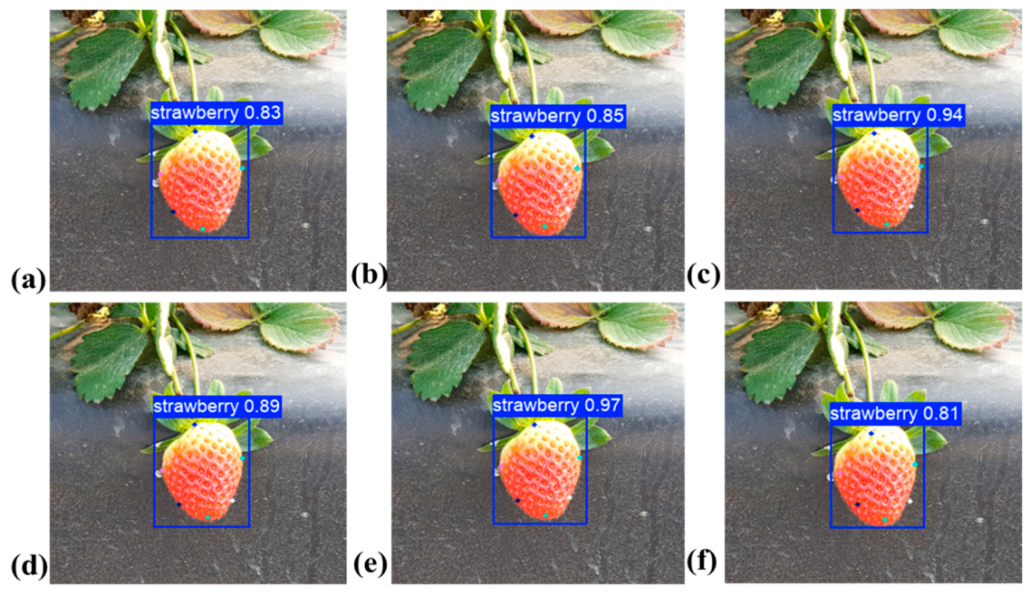
Qualitative comparison of keypoint prediction results from different pose models on a representative occlusion case. (a) YOLOv11n-pose baseline; (b) YOLOv8n-pose; (c) YOLOv11s-pose; (d) YOLOv12n-pose; (e) YOLOv26n-pose; (f) StrawPose-Lite. All sub-images are displayed with the same crop size and visual scale. K0 denotes the pedicel–fruit junction, whereas the auxiliary keypoints provide geometric context for width, curvature, and longitudinal extent.
Figure 9.
Qualitative comparison of keypoint prediction results from different pose models on a representative occlusion case. (a) YOLOv11n-pose baseline; (b) YOLOv8n-pose; (c) YOLOv11s-pose; (d) YOLOv12n-pose; (e) YOLOv26n-pose; (f) StrawPose-Lite. All sub-images are displayed with the same crop size and visual scale. K0 denotes the pedicel–fruit junction, whereas the auxiliary keypoints provide geometric context for width, curvature, and longitudinal extent.
Figure 10.
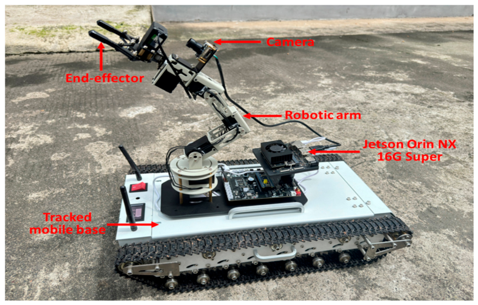
Robotic platform used for edge deployment evaluation of StrawPose-Lite.
Figure 10.
Robotic platform used for edge deployment evaluation of StrawPose-Lite.
Figure 11.
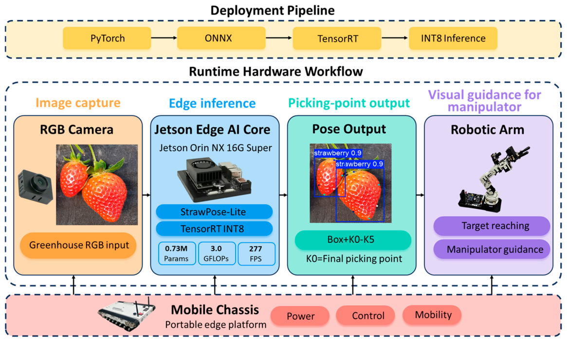
Edge deployment framework and runtime workflow of StrawPose-Lite for strawberry picking point prediction, including image acquisition, preprocessing, network inference, and postprocessing outputs.
Figure 11.
Edge deployment framework and runtime workflow of StrawPose-Lite for strawberry picking point prediction, including image acquisition, preprocessing, network inference, and postprocessing outputs.
Figure 12.
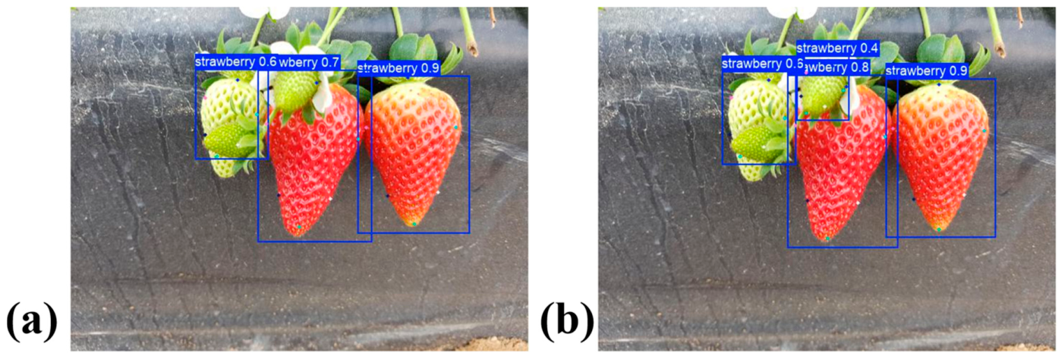
Qualitative comparison between the YOLOv11n-pose baseline and StrawPose-Lite under a representative field scene. (a) YOLOv11n-pose baseline; (b) StrawPose-Lite. The scene contains overlapping fruits, mixed maturity, and partial occlusion near the pedicel–fruit junction.
Figure 12.
Qualitative comparison between the YOLOv11n-pose baseline and StrawPose-Lite under a representative field scene. (a) YOLOv11n-pose baseline; (b) StrawPose-Lite. The scene contains overlapping fruits, mixed maturity, and partial occlusion near the pedicel–fruit junction.
Table 1.
Definitions and geometric roles of the six keypoints.
Table 1.
Definitions and geometric roles of the six keypoints.
| Keypoint | Anatomical Meaning | Geometric Role | Used for Final Picking Point |
|---|
| K0 | Pedicel–fruit junction | Final visual picking point | Yes |
| K1 | Right peak point | Right-side width constraint | No |
| K2 | Right curvature point | Right contour curvature constraint | No |
| K3 | Bottom point | Longitudinal stability constraint | No |
| K4 | Left curvature point | Left contour curvature constraint | No |
| K5 | Left peak point | Left-side width constraint | No |
Table 2.
Dataset composition, instance statistics, and usage in this study.
Table 2.
Dataset composition, instance statistics, and usage in this study.
| Dataset | Split | Images | Strawberry Instances | Total Keypoint Slots | Valid Keypoints | Validity Rate | Role | Usage |
|---|
| StrawDI_Db1 | Train | 2790 | 6863 | 41,178 | 39,460 | 95.82% | Public development set | Training |
| StrawDI_Db1 | Validation | 310 | 763 | 4578 | 4360 | 95.24% | Public development set | Validation, convergence analysis, ablation study, and model comparison |
| StrawDI_Db1 | Total | 3100 | 7626 | 45,756 | 43,820 | 95.79% | Public development set | Core algorithmic experiments |
| Field-collected set | Field | 1200 | 2952 | 17,712 | 16,740 | 94.52% | Independent field set | Edge deployment evaluation only |
| Total | — | 4300 | 10,578 | 63,468 | 60,560 | 95.42% | — | Training, validation, and deployment-oriented evaluation |
Table 3.
Experimental hardware and training settings.
Table 3.
Experimental hardware and training settings.
| System | Ubuntu 22.04 |
|---|
| Python | 3.9 |
| PyTorch | 2.9.0 |
| CUDA | 12.8 |
| GPU | NVIDIA RTX 5090 (32 GB) |
| CPU | Intel Xeon Platinum 8470Q |
| RAM | 90 GB |
| Size | 640 × 640 |
| Epoch | 100 |
| Batch size | 64 |
Table 4.
Ablation results of different module combinations based on the YOLOv11n-pose baseline. The keypoint branch enhancement module consists of P3–P5 adaptive fusion, gated P2 feature injection, and SimAM refinement. Bold values indicate the numerically best result in each column under the same experimental protocol; no additional threshold was applied.
Table 4.
Ablation results of different module combinations based on the YOLOv11n-pose baseline. The keypoint branch enhancement module consists of P3–P5 adaptive fusion, gated P2 feature injection, and SimAM refinement. Bold values indicate the numerically best result in each column under the same experimental protocol; no additional threshold was applied.
| Modules | Pose Metrics | Params (M) | GFLOPs | Size (MB) | FPS |
|---|
| Baseline | ADown | C3Ghost | Keypoint Branch Enhancement Module | P (%) | R (%) | mAP@0.5 (%) | mAP@0.5:0.95 (%) |
|---|
| √ | | | | 82.90 | 89.60 | 92.70 | 78.40 | 2.66 | 6.60 | 5.39 | 167 |
| √ | √ | | | 82.90 | 91.70 | 92.90 | 77.90 | 0.64 | 2.40 | 1.52 | 291 |
| √ | | √ | | 83.20 | 91.70 | 92.80 | 77.80 | 0.71 | 2.70 | 1.65 | 285 |
| √ | | | √ | 81.80 | 94.10 | 93.10 | 78.30 | 0.81 | 3.50 | 1.94 | 268 |
| √ | √ | √ | | 80.90 | 92.20 | 93.10 | 78.00 | 0.63 | 2.30 | 1.52 | 293 |
| √ | √ | | √ | 82.90 | 91.30 | 93.20 | 77.90 | 0.74 | 3.10 | 1.80 | 276 |
| √ | | √ | √ | 84.80 | 90.00 | 93.20 | 78.00 | 0.81 | 3.40 | 1.94 | 270 |
| √ | √ | √ | √ | 84.00 | 90.50 | 93.70 | 79.20 | 0.73 | 3.00 | 1.80 | 279 |
Table 5.
Repeated training stability and statistical significance analysis between YOLOv11n-pose and StrawPose-Lite. Note: Bold values indicate the better result between YOLOv11n-pose and StrawPose-Lite.
Table 5.
Repeated training stability and statistical significance analysis between YOLOv11n-pose and StrawPose-Lite. Note: Bold values indicate the better result between YOLOv11n-pose and StrawPose-Lite.
| Model | Pose mAP@0.5 (%) | Pose mAP@0.5:0.95 (%) |
|---|
| YOLOv11n-pose | 92.727 ± 0.110 | 78.407 ± 0.105 |
| StrawPose-Lite | 93.710 ± 0.115 | 79.200 ± 0.110 |
| p-value | 0.00044 | 0.00084 |
Table 6.
Comparison of StrawPose-Lite with representative state-of-the-art pose models under identical experimental settings. Note: Bold values indicate the best result in each column.
Table 6.
Comparison of StrawPose-Lite with representative state-of-the-art pose models under identical experimental settings. Note: Bold values indicate the best result in each column.
| Model (Pose) | Params (M) | GFLOPs | P (%) | R (%) | mAP@0.5
(%) | mAP@0.5:0.95
(%) | Size
(MB) | FPS |
|---|
| YOLOv11n-pose baseline | 2.66 | 6.60 | 82.90 | 89.60 | 92.70 | 78.40 | 5.39 | 167 |
| YOLOv8n-pose | 3.09 | 8.40 | 83.60 | 90.60 | 93.00 | 78.40 | 6.13 | 142 |
| YOLOv11s-pose | 9.70 | 22.3 | 84.70 | 88.10 | 93.20 | 79.40 | 18.8 | 86 |
| YOLOv12n-pose | 2.64 | 6.60 | 82.90 | 91.80 | 92.90 | 77.60 | 5.43 | 158 |
| YOLOv26n-pose | 2.68 | 6.70 | 83.70 | 90.40 | 93.00 | 77.90 | 5.46 | 171 |
| StrawPose-Lite | 0.73 | 3.00 | 84.00 | 90.50 | 93.70 | 79.20 | 1.80 | 279 |
Table 7.
Comparison of StrawPose-Lite with representative MMDetection-based backbones in accuracy and computational efficiency. Note: Bold values indicate the best result in each column.
Table 7.
Comparison of StrawPose-Lite with representative MMDetection-based backbones in accuracy and computational efficiency. Note: Bold values indicate the best result in each column.
| Model | mAP@0.5:0.95 (%) | mAP@0.5 (%) | GFLOPs | Params (M) |
|---|
| ResNet-101 | 65.00 | 83.00 | 336 | 63.00 |
| Swin | 82.00 | 94.00 | 342 | 60.00 |
| CSWin | 84.00 | 96.00 | 339 | 54.00 |
| StrawPose-Lite | 79.20 | 93.70 | 3.0 | 0.73 |
Table 8.
Latency breakdown of YOLOv11n-pose and StrawPose-Lite on Jetson Orin NX 16G Super. Note: Bold values indicate the lowest latency in each column.
Table 8.
Latency breakdown of YOLOv11n-pose and StrawPose-Lite on Jetson Orin NX 16G Super. Note: Bold values indicate the lowest latency in each column.
| Model (Pose) | Format | Preprocess (ms) | Inference (ms) | Postprocess (ms) | Total (ms) |
|---|
| YOLOv11n-pose baseline | PyTorch | 1.1 | 14.08 | 1.3 | 16.48 |
| YOLOv11n-pose baseline | TensorRT FP16 | 0.9 | 5.68 | 0.9 | 7.48 |
| YOLOv11n-pose baseline | TensorRT INT8 | 0.9 | 4.76 | 0.9 | 6.56 |
| StrawPose-Lite | PyTorch | 1.0 | 9.62 | 1.0 | 11.62 |
| StrawPose-Lite | TensorRT FP16 | 0.7 | 4.27 | 0.7 | 5.67 |
| StrawPose-Lite | TensorRT INT8 | 0.7 | 3.61 | 0.7 | 5.01 |
Table 9.
Edge deployment results of YOLOv11n-pose baseline and StrawPose-Lite under PyTorch, TensorRT FP16, and TensorRT INT8 on the independent field dataset. The reported FPS refers to pure network inference throughput. Note: Bold values indicate the best result in each column.
Table 9.
Edge deployment results of YOLOv11n-pose baseline and StrawPose-Lite under PyTorch, TensorRT FP16, and TensorRT INT8 on the independent field dataset. The reported FPS refers to pure network inference throughput. Note: Bold values indicate the best result in each column.
| Model (Pose) | Format | P (%) | R (%) | mAP@0.5 (%) | mAP@0.5:0.95 (%) | Pure Network Inference FPS |
|---|
| YOLOv11n-pose baseline | PyTorch | 80.40 | 85.80 | 90.20 | 72.60 | 71 |
| YOLOv11n-pose baseline | TensorRT FP16 | 80.20 | 85.60 | 90.00 | 72.40 | 176 |
| YOLOv11n-pose baseline | TensorRT INT8 | 79.60 | 84.20 | 89.00 | 69.90 | 210 |
| StrawPose-Lite | PyTorch | 82.10 | 87.40 | 91.60 | 74.10 | 104 |
| StrawPose-Lite | TensorRT FP16 | 81.90 | 87.20 | 91.40 | 73.90 | 234 |
| StrawPose-Lite | TensorRT INT8 | 81.30 | 85.80 | 90.40 | 71.60 | 277 |




 ,
,