Article

Dispersion Modelling and Measurements to Assess Odour Impact of Multi-Storey Pig Houses in Complex Terrain

1
School of Optical, Mechanical and Electrical Engineering, Zhejiang Agriculture & Forestry University, Hangzhou 311300, China
2
College of Biosystems Engineering and Food Science, Zhejiang University, Hangzhou 310058, China
*
Author to whom correspondence should be addressed.
Agriculture 2026, 16(11), 1181; https://doi.org/10.3390/agriculture16111181
Submission received: 7 April 2026 / Revised: 11 May 2026 / Accepted: 25 May 2026 / Published: 28 May 2026
(This article belongs to the Section Farm Animal Production)

Abstract

Multi-storey pig houses (MSPHs) have been built as a land-efficient solution for intensive swine production in China, but can cause odour nuisances for and complaints from nearby residents. In this study, air quality measurements and dispersion modelling using AERMOD were conducted to quantify the odour impact around a swine barn with two MSPHs equipped with air scrubbers in complex terrain. The field measurements showed strong seasonal fluctuations. The two MSPHs were modelled as eight elevated point sources, incorporating building downwash effects, to determine the setback distances between the barn and residential areas located 1 km away to the north. The results showed a pronounced north–south plume elongation, which was consistent with the prevailing wind direction and the valley topography. Using the odour impact criteria (OIC) with an odour occurrence-free frequency of 99.5%, the maximum setback distance in the north decreased from >4000 m to 951 m with the odour concentration threshold increasing from 1 to 10 OU/m3. The summer-only worst-case scenario yielded larger impact zones (>4000 m for 1–2 OU/m3; 2554 m for 10 OU/m3 at 99.5%), indicating that warm-season exposure should be considered when assessing residential risk. Under the current national OIC of 10 OU/m3 for residential areas, the modelled setback distance (951 m at 99.5%) indicated that the communities were situated outside the odour impact zone, which did not align with the documented complaints, demonstrating that the 10 OU/m3 threshold is lenient for high-density MSPH operations.

1. Introduction

As the largest producer and consumer of pork, China has promoted the construction of multi-storey pig houses (MSPHs) for large-scale swine operations in densely populated areas in recent years. While these vertically stacked facilities optimize land use by concentrating large animal populations within a compact building footprint, this configuration can fundamentally alter the spatial distribution and magnitude of odour emissions compared to conventional single-storey barns. A typical MSPH is usually equipped with a mechanical ventilation system for each floor and an extended shaft to collect and discharge the exhaust air at the rooftop [1]. Moreover, end-of-pipe mitigation technologies are commonly implemented in MSPHs for odour control, such as wet acid scrubbers, bioscrubbers and biofilters [2,3]. However, the intensive production in MSPHs still aggravates odour problems within their neighbourhoods. It was reported that odour issues accounted for nearly 50% of air pollution complaints in China, with the livestock sector contributing to about 11% of odour nuisances from 2018 to 2020 [4]. Therefore, there is a need to assess the odour impact of MSPHs, a new type of swine housing facility, on their surrounding communities to avoid odour annoyances, and to provide information about strategies for the management of odour control in MSPHs.
A setback distance is commonly established to mitigate the potential negative impacts of odour emissions source on nearby communities, which can be affected by the land-use category [5]. Sensitive receptors, such as residential areas, are more susceptible to experiencing nuisances due to their proximity to the sources and higher population density driven by rapid urbanization [6,7]. Atmospheric dispersion models are widely used to determine the setback distance by calculating the hourly ambient odour concentrations at the surrounding receptors. The modelled odour concentrations are then evaluated by odour impact criteria (OIC), which typically combine a concentration threshold with a percentile compliance level [8]. Generally, OIC are regulated by national or regional environmental agencies or other governmental authorities. Various national OIC are summarized by Brancher et al. [9].
Researchers have used various dispersion models to simulate the spatial distribution of air pollutants and assess the impact on neighbourhoods [10,11,12,13], such as AERMOD [14], AODM [15] and CALPUFF [16]. It is difficult to define a dispersion model with better performance for the prediction of odour distribution from livestock production, since these gas emissions are highly site-specific. AERMOD, one of the widely used models, is a Gaussian dispersion model suitable for simple (flat) or complex terrain scenarios within urban and rural areas affected by multiple surface and elevated emissions sources [17,18]. Tartakovsky et al. [19] compared the concentrations of particulate emissions in hilly terrain predicted by AERMOD and CALPUFF and found that AERMOD had better performance for complex terrain scenarios. Wu et al. [20] determined the maximum separation distances for a 300-head dairy farm as 655 m, with an exceedance probability of 15% based on AERMOD, and investigated the selection of an appropriate meteorological station that best represented the area surrounding the farm. Huang and Guo [21] used AERMOD to determine the setback distances for different commercial barns in the Canadian Prairies, and the results showed the maximum setback distances decreased from 1941 m to 641 m for the layer barn and from 980 m to 320 m for the broiler barn while the odour concentration thresholds increased from 1 OU/m3 to 6 OU/m3 with an occurrence-free frequency of 99.5%. Although AERMOD has been widely applied to conventional single-storey livestock barns with near-ground or low-elevation sources on flat terrain [20,21,22,23], no published study has applied a dispersion model to MSPHs. Unlike conventional barns, MSPHs discharge exhaust air from elevated and elongated rectangular shaft openings at the rooftop, producing a source configuration fundamentally different from previously modelled livestock facilities. Additionally, most MSPHs are located in topographically complex environments, such as valleys or hilly regions, due to limited land and urbanization. Different from simple flat terrain, the dispersion of odour in such environments is strongly influenced by local atmospheric dynamics and the complex terrain conditions.
To address this critical research gap, this study investigated the spatial odour distribution of a commercial barn with two MSPHs located in complex terrain. We hypothesized that the exhaust from the MSPHs would create highly directional odour impact zones due to its interaction with local topographic forcing in complex terrain, and the choice of OIC would substantially influence the resulting setback distance recommendations. The specific objectives of this study were: (1) to characterize the seasonal variability in odour emissions from MSPHs equipped with acid scrubbers; (2) to evaluate the spatial patterns of odour dispersion around MSPHs in complex terrain using AERMOD; and (3) to evaluate the efficacy of various odour impact criteria (OIC) against national standards to determine appropriate setback distances.

2. Materials and Methods

2.1. Description of the Study Site

The study site is a commercial swine barn located in Shaoxing (120.47° E, 30.01° N), Zhejiang Province, China, which is a hilly region with a humid subtropical climate. It has two four-storey houses with a total capacity of 45,000 pigs. Floors 1 and 2 of MSPH 1 are used for keeping fattening pigs with an average weight of 75 kg; floors 3 and 4 of MSPH 1 are designed for nursery pigs and farrowing sows with average weights of 10 kg and 150 kg, respectively. A scraper system is applied on floor 2 of MSPH 1, and manure flushing systems are applied to the remaining floors. In MSPH 2, floor 1 is designed for fattening pigs housing and is equipped with a manure flushing system; floors 2–3 are used for keeping fattening pigs and are equipped with a scraper system; and floor 4 is used for gestating sows with a scraper system. The average weights of the fattening pigs and gestating sows in MSPH 2 are 75 kg and 135 kg, respectively. Automatic feeding and watering systems are applied to all floors of two MSPHs.
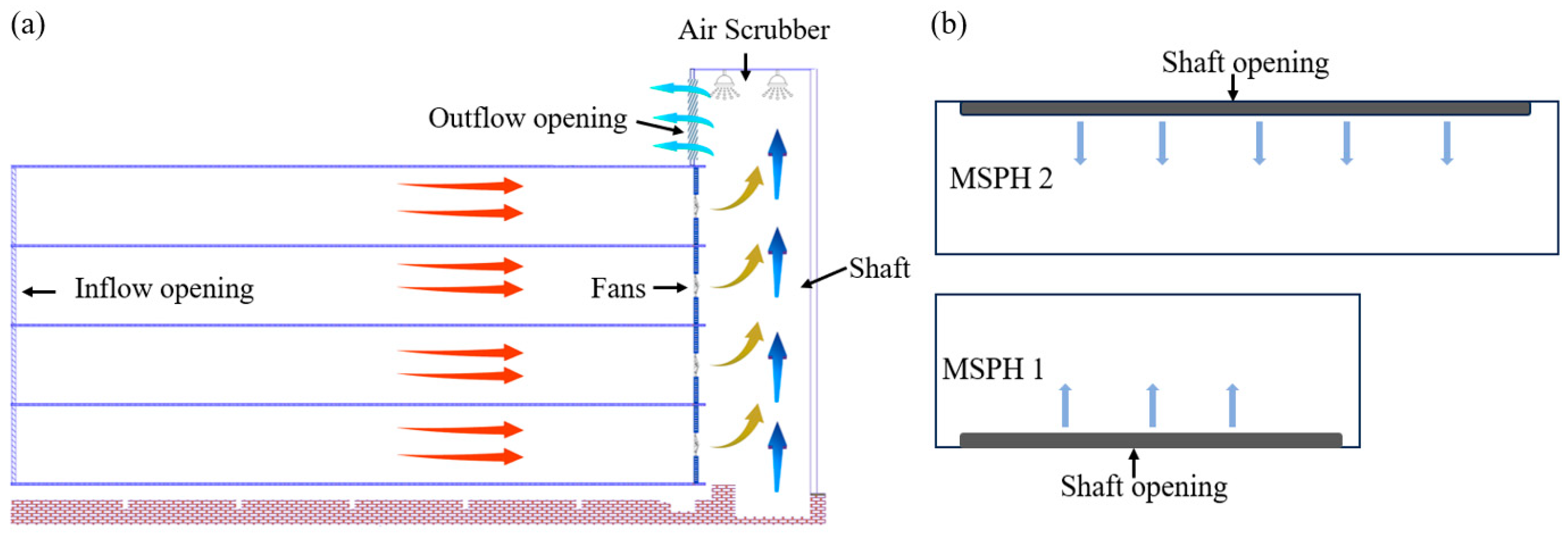
The two MSPHs operate year-round and adopt the same automated tunnel ventilation system (Figure 1a). The fans are installed at the opposite endwall to the inlet and the air is drawn out horizontally to a shaft. The shaft collects the exhausted air and allows for the release of the outgoing air from each floor from the upper side of the shaft. Before release, the air is treated by an acid scrubber, equipped with spray nozzles and nylon mesh filters on the top of the shaft, to remove ammonia and particulate matter, and then it is released horizontally at the rooftop. The two shaft openings face each other and the distance between them is 107.0 m (Figure 1b). The inside dimensions of the shaft openings are 133.0 m long by 2.7 m high for MSPH 1, and 194.0 m long by 2.7 m high for MSPH 2. The overall height of the shafts is 18.2 m, while the buildings themselves are 15.1 m high. The manure treatment facilities in the swine barn, including the anaerobic sedimentation tank and solid–liquid separation unit, were not considered as odour emissions sources in this paper, since they operate as closed systems equipped with a waste gas treatment infrastructure. It should be noted that complaints about odour nuisances from the swine barn have been made by the nearby residents according to the local government.
The farm’s operational data were obtained directly from the farm manager through a structured interview and documentation review conducted prior to and during the experiments. The shaft dimensions and fan specifications were verified through on-site measurements and cross-checked against engineering drawings provided by the farm operator.

2.2. Odour Sampling and Measurements

The sampling and measurements were conducted for typical months in each season (March, August, October and December) in 2023. However, the sampling was restricted to one representative day per season because of the strict biosecurity protocols of commercial Chinese swine farms. During the experimental day, four replicate samples were collected at four different spots of the MSPHs’ shaft openings across three sampling events, spaced at three-hour intervals, resulting in a total of 12 samples per shaft per day. The air samples were collected using 10-L Tedlar® air bags (Hongpu Instrument Technology Co., Ltd., Ningbo, Zhejiang, China) and were transported to the olfactometry laboratory for analysis within 24 h. Measurements of odour concentration were conducted with trained panellists in accordance with CEN standards [24].
Based on the measurements, the odour emission rates of the MSPHs were calculated by Equation (1):
E R = Q   ×   O C
where ER is the odour emission rate, OU/s; Q is the ventilation rate, m3/s; and OC is the odour concentration of exhausted air emitted from the shaft opening, OU/m3. The ventilation rate was calculated by the exit velocity of air and the area of the shaft opening. The exit velocity of air emitted from the MSPHs shaft openings was measured by an air velocity meter (9565-P, TSI Incorporated, Shoreview, MN, USA).
The ammonia, temperature, and relative humidity (RH) were measured using a portable multi-channel gas detector (GT-903, Korno Co., Ltd., Shenzhen, Guangdong, China). Concentrations of particulate matter (PM), i.e., TSP, in the exhaust and treated air were measured on-site using a highly sensitive Aerosol monitor (Model pDR1500, Thermo-Scientific, Waltham, MA, USA).

2.3. Model Configuration

Three datasets were prepared for the AERMOD (v24142) modelling system, including the source odour emission data, meteorological data and terrain data. The modelling system consists of one main module (AERMOD) and two pre-processors (AERMET and AERMAP). Firstly, AERMET was used to process the meteorological data and generate meteorological data profiles, and AERMAP was applied to process the terrain data and generate receptor grids for AERMOD. Then, these data profiles and source odour emission data were input into the main program, AERMOD, to predict the odour dispersion around the swine barn.

2.3.1. Source Emission Data

Since the gas from the shafts of the MSPHs was treated to control odour before emission, the emission rates were considered constant, using the average values of all seasons. The two MSPHs were treated as point source types in the AERMOD model configuration, according to the U.S. EPA [25], since the AREA and VOLUME source types do not allow for horizontal release and consideration of building downwash. It should be noted that a specific “POINTHOR” source type was adopted since the air was released horizontally from the shaft openings (Figure 1). The point source modelling requires the emission rate, release height, gas exit temperature, gas exit velocity and inside diameter of the point source as the inputs. The release height was defined as 16.45 m (15.1 m for the building height and 1.35 m for the centre of shaft opening). Due to the elongated and rectangular shape of the exhaust shaft openings, it would be unreasonable and inaccurate to model each opening as one single point source. Therefore, each shaft was divided into N equally sized segments, and an equivalent diameter computed from the cross-sectional area was assigned to each segment. The segments of each shaft had the same horizontal exit velocity, and 1/N of the total odour emission rate. The challenge of source configuration was the choice of number of point sources to represent the initial horizontal spread of the emission plume. A sensitivity analysis was conducted to investigate the influence of two point-source configurations: (a) 3 + 5 segments: three point sources for MSPH 1 and five for MSPH 2; (b) 7 + 10 segments: seven point sources for MSPH 1 and ten for MSPH 2. Figure S1 exhibits an example of modelled odour concentrations at the receptors from 0 m to 4000 m away in the north direction using the two point source configurations. Condition (a) was then adopted for model configuration due to its simplicity and computational efficiency.

2.3.2. Meteorological Data

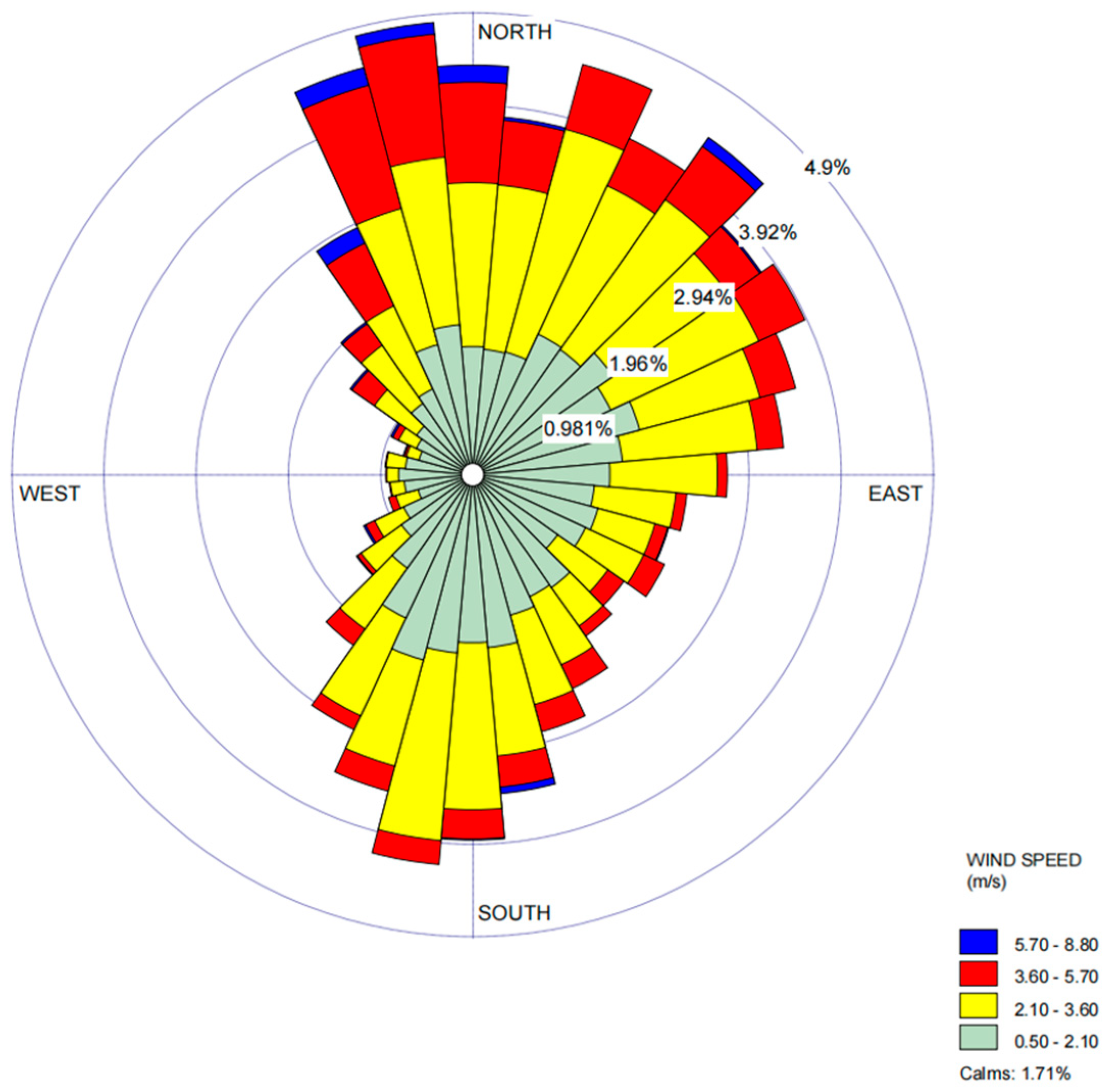
The meteorological data, including the surface weather data from the closest weather station, Shaoxing Station, and the upper-air sounding data from the ERA5 Database were gathered for the year 2023. Then, two meteorological data profiles were generated by AERMET and later used as inputs for the AERMOD dispersion model. Figure 2 shows that the mean wind velocity in the study area was 2.28 m/s, with prevailing wind directions of north and south and SSE. The calm wind frequency was 1.71%, indicating that the site experienced predominantly non-calm conditions and the plume was transported consistently throughout the year.

2.3.3. Terrain Data

The terrain elevation was obtained using the FABDEM V1-2 database with a spatial resolution of 30 m, and then was processed by AERMAP for the terrain data profile. The building downwash effects were considered due to the complex structure of two 4-storey MSPHs with exhaust shaft openings on the roof. The BPIPPRM downwash algorithm, with the input of the height and width of the two MSPHs, was used to account for the specific aerodynamic influences of the multi-storey structures. The modelling protocol followed the regulatory options set in the U.S. EPA Guideline on Air Quality Models [26].

2.3.4. Receptors

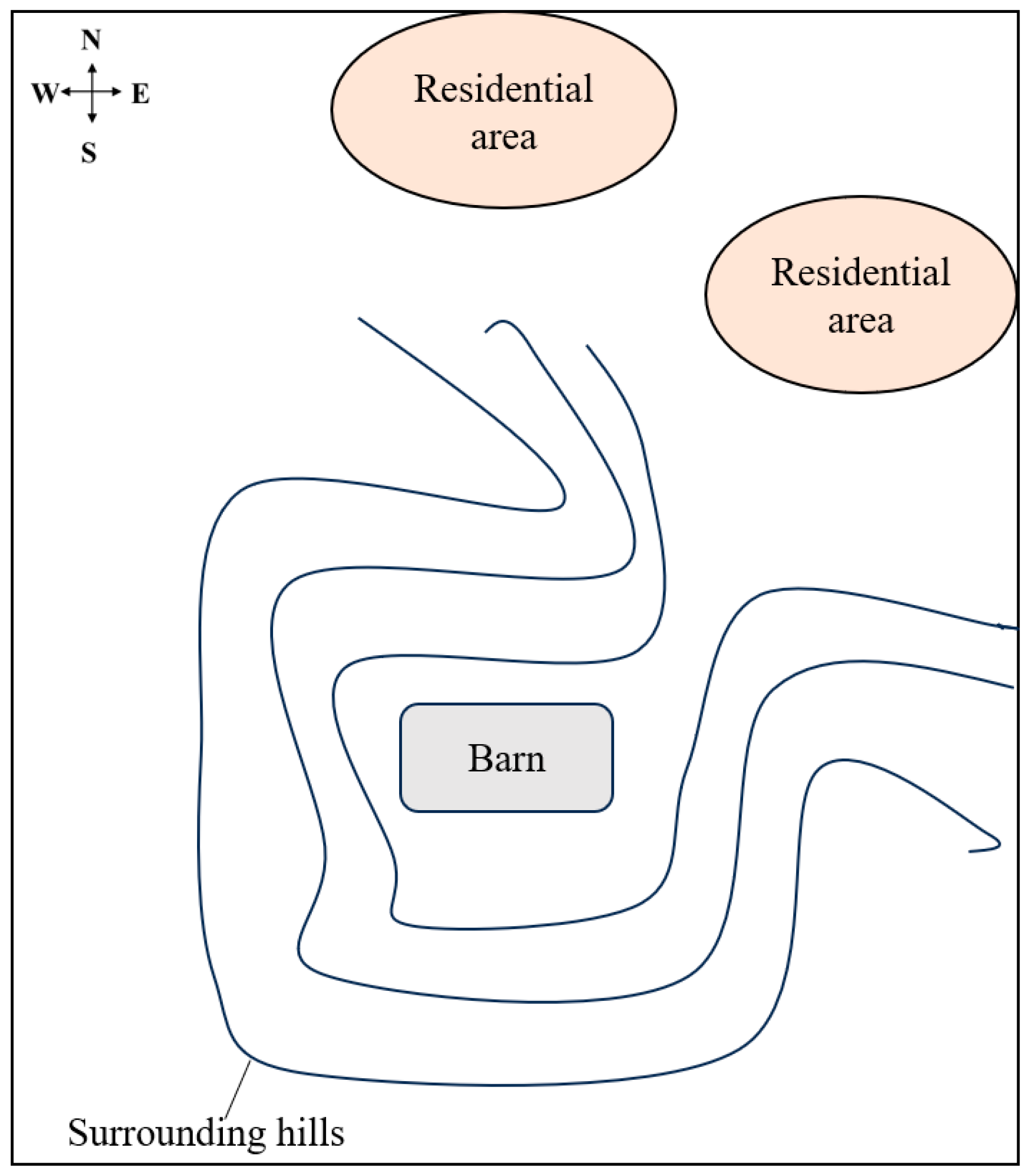
The model domain covered 8 km × 8 km centring around the pig barn, which is a hilly suburban area with arable land, and residential and industrial units. Figure 3 illustrates that the swine barn with MSPHs is surrounded by forested hills rising about 50 m above the barn on the western, southern, and eastern sides, leaving only the northern corridor open toward residential areas, which are approximately 1 km to the northeast and 1.5 km to the north. A total of 6560 receptors with 100 m spacing (source excluded) were placed for the model. The height of each receptor was set at 1.5 m to simulate human breathing height.
After running the AERMOD modelling system, the predicted hourly odour concentrations were obtained at each receptor for the entire year. The annual average odour concentrations of the receptors were calculated using Python 3.12 and were input into Surfer 29 (Golden Software, Golden, CO, USA) to generate the concentration contours. Moreover, the odour occurrence-free frequency (the percentage of hours when the odour concentration did not exceed the OIC threshold) for each receptor was calculated using Python, and was plotted by Surfer 29.

3. Results

3.1. Odour Measurements

The results of odour emission rate (ER), air exit velocity (EV), as well as NH3 and PM concentrations of the samples collected from the two MSPHs shaft openings are shown in Table 1. The odour emission rate during the summer month reached 55,035.67 OU/s for MSPH 1 and 68,827.32 OU/s for MSPH 2, which are about five times higher compared to winter levels. The air exit velocity from the shaft openings of MSPHs also showed a seasonal peak in summer, i.e., 1.46 m/s for MSPH 1 and 1.58 m/s for MSPH 2. The temperature of the test day in summer was 38°C, which was much higher than the temperature in winter (10 °C). The ammonia concentration showed a similar trend as the odour emission rate, peaking at 1.00 mg/m3 (MSPH 1) and 0.95 mg/m3 (MSPH 2) in the summer and showing low concentrations in winter (0.09 mg/m3 for MSPH 1 and 0.15 mg/m3 for MSPH 2). However, the PM concentrations exhibited the highest values in winter (368.71 μg/m3 for MSPH 1 and 421.39 μg/m3 for MSPH 2). The measured odour emission rate and concentrations of NH3 and PM had similar values in spring time and winter time. It should be noted that the average temperature of the test day in winter (December) was 10°C, close to the average temperature in spring (March, 13 °C). The average air exit velocities and 1/N of the average odour emission rates were used for model inputs, as described in Section 2.3.1.

3.2. Modelled Odour Concentration

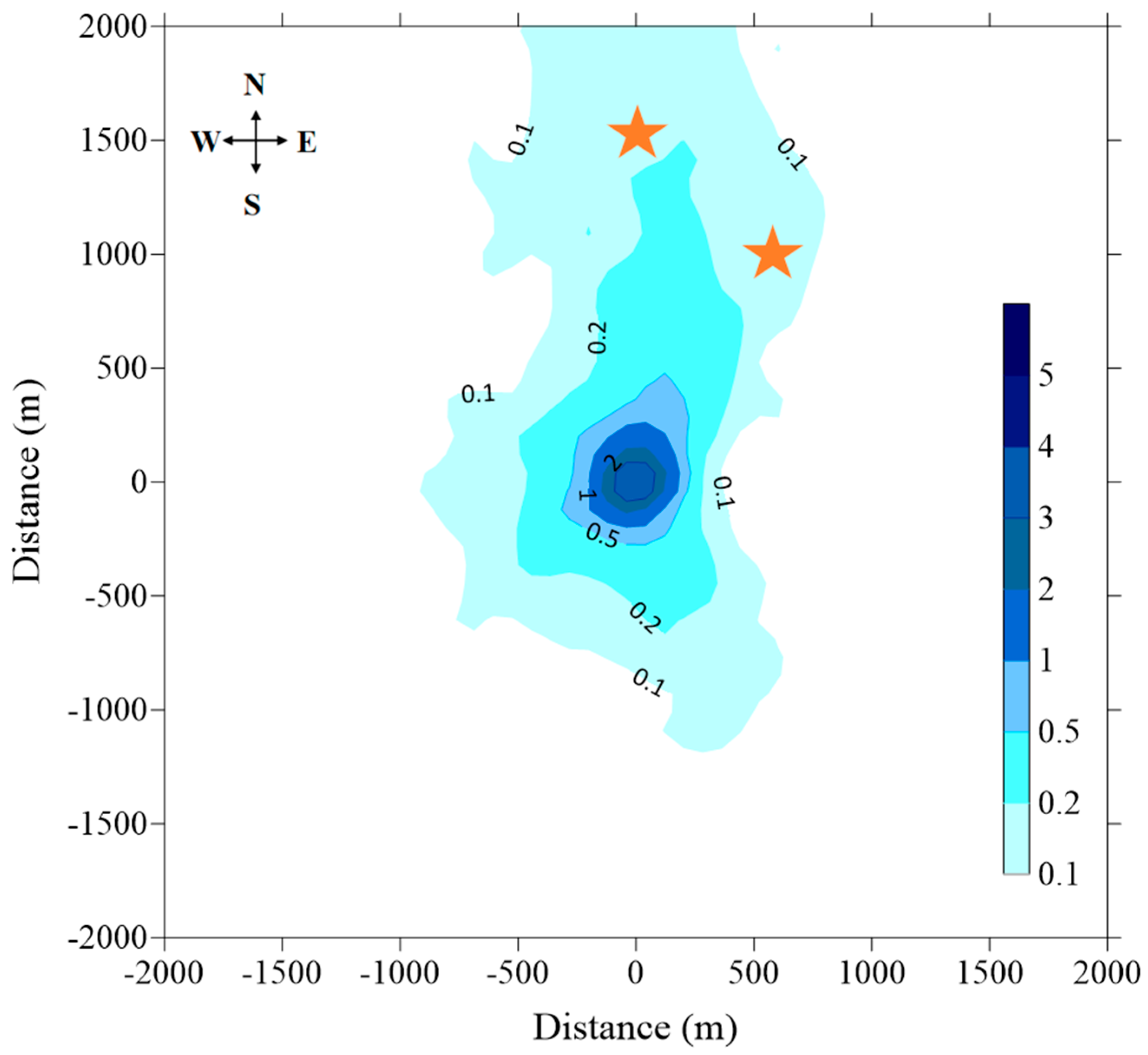
The source configuration (three point sources for MSPH 1 and five for MSPH 2) was used for the model since no significant differences were found between the two conditions of point source numbers (Figure S1). The annual average concentrations of the receptors were determined based on the hourly concentrations for an entire year predicted by the AERMOD model. Figure 4 shows the annual average concentration contour for the swine barn, which demonstrates a distinct spatial distribution characterized by north–south elongation. This reflects the impact of wind distribution (Figure 2) on the odour concentrations. The annual average odour concentration showed very low values around the barn. The odour travel distance reached 2281 m to the north of the barn using an odour concentration limit of 0.1 OU/m3, 1485 m to the north for 0.2 OU/m3, 463 m to the north for 0.5 OU/m3, and 264 m to the north for 1 OU/m3. The results of annual average odour concentration indicate that the odour impact area is highly directional (north–south) and asymmetric around the barn. Two residential areas, noted in Figure 4, were exposed to odour with an annual concentration of 0.1 OU/m3. However, the setback distances cannot be determined by the annual average odour concentration. The setback distances are derived from the odour occurrence-free frequency in the following Section 3.3.

3.3. Setback Distances

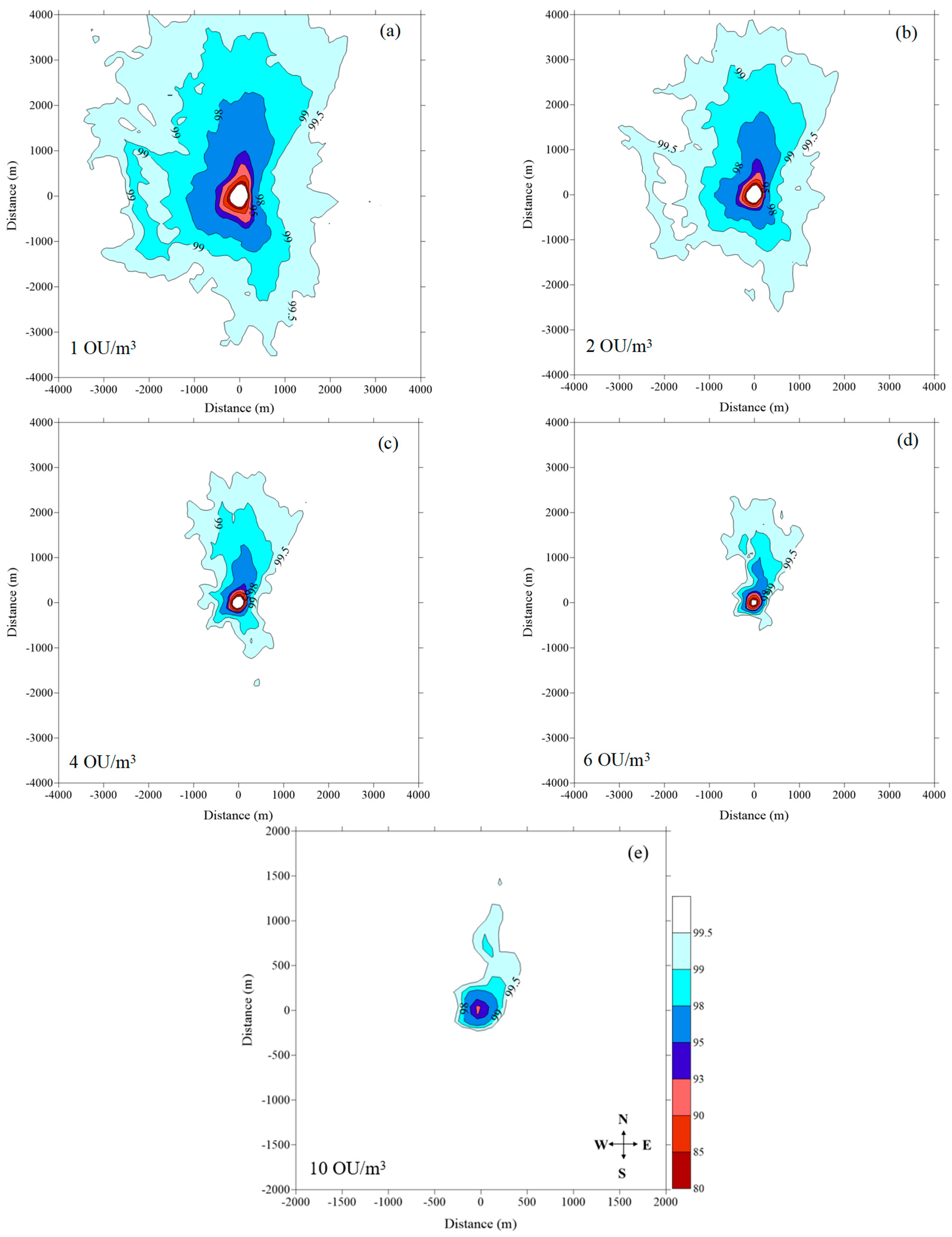
To determine the setback distance between odour sources and residential areas, the selection of OIC is critical, including an odour threshold concentration and the occurrence-free probability of this threshold. In China, a constant odour concentration of 10 OU/m3 is used as the OIC for residential areas, which is higher than in many countries. Most countries use a constant occurrence-free probability and modify the odour concentration threshold to adjust the OIC to the protection level [5]. To better assess the odour impact, five thresholds with an averaging time of 1 h and odour occurrence-free frequency of 99.5% were selected for this study: 1, 2, 4, and 6 OU/m3, adopted from Huang and Guo [21]; and 10 OU/m3 from Chinese national standards. Sommer-Quabach et al. [5] found that a low odour concentration and higher exceedance probability, in other words, a lower occurrence-free frequency, are more suitable for OIC. Therefore, odour occurrence-free frequencies in range of 80–99.5% were used to generate the contours for the comparisons of setback distances (Figure 5). The odour occurrence-free frequency contours under the five OIC thresholds of 1, 2, 4, 6 and 10 OU/m3 all showed the greatest impact in the northward direction, with a north and northwest elongated and asymmetric shape. The directional pattern was consistent with the prevailing wind direction and the valley topography discussed in Section 3.2. Some isolated contour “islands”, shown in Figure 5, represent the localized receptor locations where the odour-free frequency was slightly below the surrounding values, and could be attributed to the plume’s impaction on the surrounding complex topography.
Using the most stringent criterion of 1 OU/m3, the 99.5% odour-free frequency contour indicates that the maximum setback distance for the swine barn with MSPHs to the north was over 4000 m, which exceeded the study area of receptors. With the odour threshold increasing from 1 to 10 OU/m3, the setback distance gradually decreased to 951 m in the north. Only the four major directions (north, south, west and east) were considered in terms of the setback distances. The setback distances determined for the four directions under different odour thresholds, with odour occurrence-free frequencies of 99.5%, 99.0% and 98.0%, are listed in Table 2. The odour impact area decreased when the odour occurrence-free frequencies decreased from 99.5% to 80% across all evaluated odour thresholds. The setback distances fort frequencies below 98% were not presented because their contours were tightly clustered aroundthe swine barn. Specifically, as the odour occurrence-free frequency decreased from 99.5% to 98%, the setback distance of the swine barn in the north decreased from >4000 m to 2126 m for an odour threshold of 1 OU/m3, from 3865 m to 1692 m for a threshold of 2 OU/m3, from 2902 m to 1040 m for a threshold of 4 OU/m3, from 2313 m to 853 m for a threshold of 6 OU/m3, and from 951 m to 225 m for a threshold of 10 OU/m3.
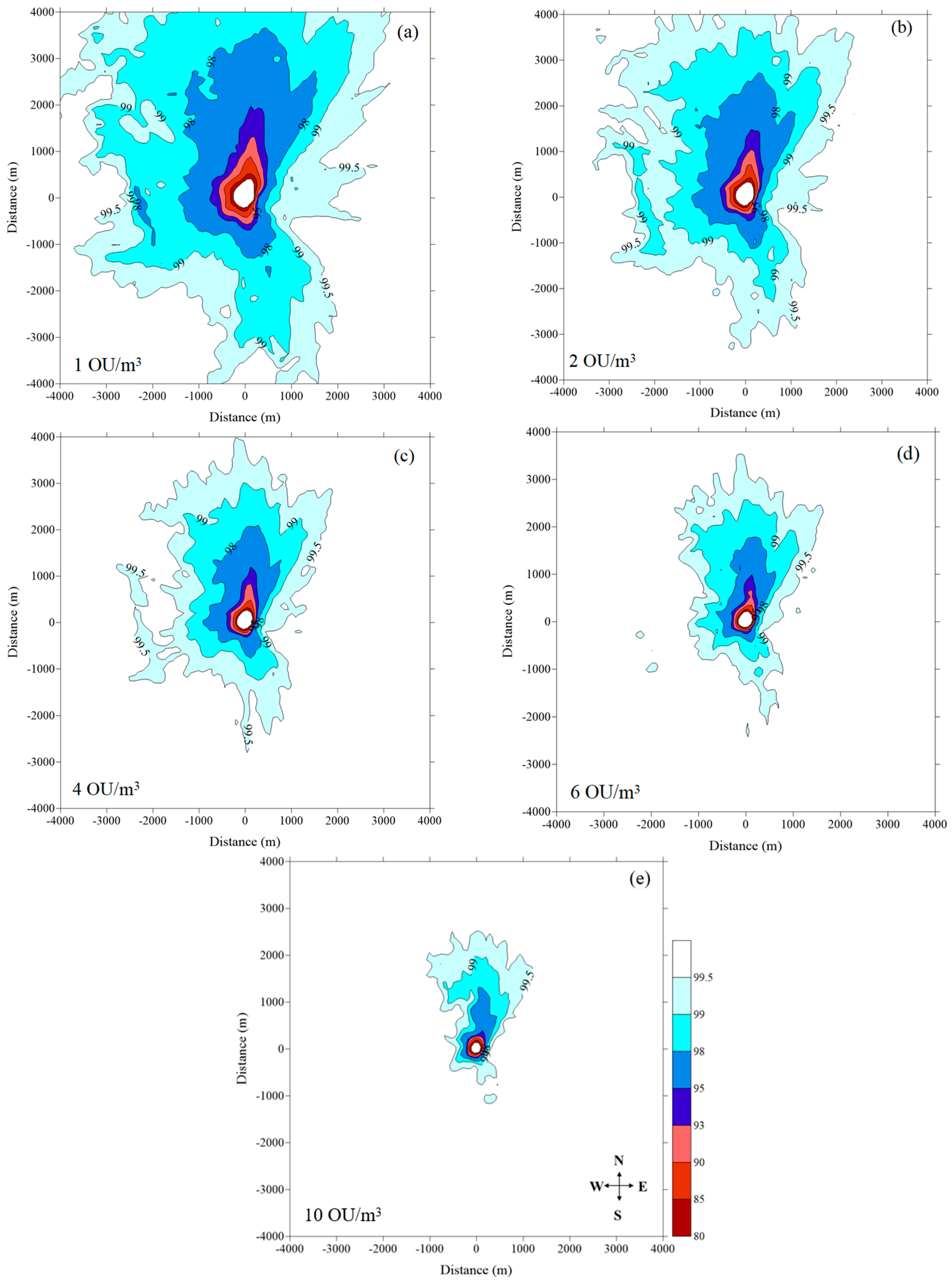
To assess the possible worst-case odour impacts, an additional AERMOD run was carried out using the measured summer emission rates (55,035.67 OU/s and 68,827.32 OU/s for MSPH 1 and 2, respectively) and the meteorological data for the summer season (from June to August) in 2023. The odour occurrence-free frequency contours under all five odour impact criteria are displayed in Figure 6. The odour impact areas in the summer-only scenario show the same northward directional pattern as the annual average analysis, but are larger than the odour impact areas using the annual average concentrations (Figure 5). For an OIC of 1 OU/m3 and 2 OU/m3 with 99.5% odour-free frequency, the maximum setback distances for the swine barn with MSPHs in the north direction are over 4000 m, which exceeds the study area (Figure 6a,b). Even using the criterion of 10 OU/m3, the setback distances in the north direction are 2554 m, 1972 m and 962 m with odour-free frequencies of 99.5%, 99% and 98%, indicating that the sensitive receptors are situated in the odour impact area during summer.

4. Discussion

The measured odour emission rates, air exit velocities, and NH3 and PM concentrations from the shaft openings of MSPHs showed strong seasonal fluctuations, which agree with Ying et al. [27]. The seasonal peak of odour emissions was strongly related to the high ventilation rate during summer time. The high air exit velocities observed in August (1.46 m/s and 1.58 m/s for MSPH 1 and MSPH 2, respectively) directly reflect the mechanical ventilation system’s planned maximum capacity cooling mode. Conversely, the significantly reduced velocities in December reflect the planned minimum ventilation strategy required to maintain indoor temperature in winter. The NH3 concentrations remained low throughout the whole year compared to untreated exhausted air from pig barns in previous studies [28,29,30], which indicates the high removal efficiency of the acid scrubber system used in the MSPHs. The PM concentrations exhibited the highest values in winter, likely due to reduced ventilation rates allowing dust to accumulate within the building environment [31].
From the annual average odour concentration contour, the plume travelled mainly in the north–south direction, slightly towards the west and almost negligibly in the east, which reflects that the wind blew least from the west and slightly from the east in the wind distribution chart. Additionally, the odour plume from the elevated emissions sources seemed to travel further than typical of those from single-storey livestock barns according to the literature [20,21]. The odour occurrence-free frequency contours under the five OIC thresholds of 1, 2, 4, 6 and 10 OU/m3 also showed the greatest impact in the northward direction, with a north and northwest elongated and asymmetric shape. Even though the annual average concentration at two sensitive receptors were very low (0.1 OU/m3), the nearby residential areas were situated within the odour impact area under an OIC of 1–6 OU/m3 and 99.0–99.5% odour occurrence-free frequency, which highlights the importance of selection of OIC.
It should be noted that the pig barn is located in a topographically complex environment, surround by hills on three sides, and the residential area with reported complaints is about 1 km away to the north. The results of odour impact area validate the initial hypothesis that the interaction between exhaust from the MSPHs and the complex valley topography creates highly directional odour impact zones. As described by Tartakovsky et al. [19], AERMOD models plumes as either directly impacting on or smoothly following the terrain. For flat terrain, an elevated plume slowly disperses downward and creates a continuous gradient. Given the complex terrain in this study, horizontal plumes from the exhaust shafts physically collide with the surrounding hills at about a 50 m elevation, potentially enhancing the concentrations at specific terrain-influenced receptor locations. The isolated contour “islands” observed in the contour plots validate this dynamic, visually representing localized plume impaction where the channelled air mass physically collided with the complex terrain [32]. The valley environment promotes cold air drainage flows under stable atmospheric conditions (usually night time and early morning), during which dense cold air pools around the barn and drains northward along the valley floor toward the residential area. This also explains the north–south elongation of the odour plume and the complaints about odour nuisance during evenings and at night. Chemel et al. [33] conducted an odour impact assessment around a landfill site in complex topography and found that local thermally driven valley winds play a key role in confining or directing air masses, which agrees with the observations in this study. The quantitative modelling by Wang et al. [34] further highlights this mechanism, demonstrating that “valley heat deficits” may restrict vertical dispersion and topographic stagnation can increase local valley pollutant concentrations by up to 30% compared to flat terrain.
The decreasing trend of odour impact zone with increasing thresholds is consistent with the results reported by Huang and Guo [21], which also validates the hypothesis that the choice of OIC substantially influences the resulting setback distance. Only when an OIC of 6 OU/m3 and 98% odour occurrence-free frequency or 10 OU/m3 were used was the residential area around the barn situated outside of the odour impact zone. The great odour impact area of the MSPHs verifies the complaints made by the nearby communities. This underscores the critical importance of OIC selection in determining regulatory setback distances. A lower odour occurrence-free frequency closer to a barn indicates more frequent odour exposure, while a higher odour-free frequency at a greater distance indicates progressively less frequent odour impact. A low odour threshold with high exceedance probability was also suggested by Piringer et al. [15] to avoid the influence of outliers on the calculation of separation distances with different models, aiming for equivalent results. Invernizzi et al. [35] used the 98th percentile level of exceedance and three concentration threshold levels (1, 3 and 5 OU/m3) to determine setback distances and discovered that the concentration threshold of 1 OU/m3 delivered the most reliable results both for separation distances and separation distances scaling factors. It should be noted that the emissions data used in the primary modelling was the annual average odour emissions rate rather than the summer peak values. The summer-only scenario yielded larger setback distances in the prevailing northward direction. This indicates that although the annual average emissions rate is the appropriate input for regulatory setback distance determination, the warm-season odour impact zone is correspondingly larger and should be considered when assessing the worst-case exposure of nearby residents.
According to the reported nuisance complaints from the residents living to the north, especially 1 km away in the northeast direction, the predicted odour dispersion was consistent with the real-world odour impact. Hog odour generates significantly greater annoyance than virtually any other common odour source and even infrequent exposure events may generate sustained community dissatisfaction [36]. Policy-making regarding setback distances quantifies the trade-off between environmental protection and land-use efficiency. MSPHs, as a new type of swine housing facility, currently use various approaches for gas emissions, as described by Wang et al. [37]. Different emissions systems, sensitivity of nearby receptors, and meteorological and terrain conditions can result in different choices of OIC and setback policies. The fact that the sensitive receptors still reported complaints despite the operation of air scrubbers in the MSPHs highlights the limitations of current odour abatement strategies. Field measurements indicate that although the acid scrubber successfully mitigated NH3 across all seasons, the high volume of air exhausted from the MSPHs still carried odorous mass, such as VOCs, which triggered nuisances. According to Han et al. [3], air scrubbing methods, mainly based on gas–liquid mass transfer, are not effective for treating hydrophobic odorous substances, such as hydrocarbons and sulphur-containing organics. For this swine barn, ethanol, acetone, toluene, and dichloromethane were the dominant compounds, with OVOCs representing the primary VOC category as reported by the other part of this project [38]. From a policy perspective, this underscores the fact that while end-of-pipe treatments are essential for mitigating chemical exposure, they cannot replace the necessity of adequate and site-specific setback distances for preventing odour nuisances from high-density MSPH operations.
A limitation of the study is that the sampling and measurements were only conducted for one selected day of typical month in each season due to strict biosecurity of commercial swine farms in China. The variability in odour emissions in different seasons may not have been fully investigated, which could have resulted in an over- or underestimation of the odour impact zone [39]. In the future, more frequent emissions measurements, such as monthly, should be carried out, as well as field measurements of ambient odour concentrations around barns to verify the modelled concentrations. Moreover, odour emissions from various MSPH sites with different topographies could be modelled to provide more information for terrain-sensitive setback policy.

5. Conclusions

This study quantified the odour impact of two MSPHs in complex valley terrain using field-measured emission rates and AERMOD dispersion modelling. The emissions from the MSPHs showed strong seasonal fluctuations governed by the mechanical ventilation rates. The modelled plume was strongly directional with a north–south elongated shape, which was consistent with the prevailing wind patterns, the valley topography and documented complaints from nearby residential areas. Using OIC with an odour occurrence-free frequency of 99.5%, the maximum setback distance in the north direction decreased from >4000 m to 951 m with the odour concentration threshold increasing from 1 to 10 OU/m3. The residential community fell outside the modelled impact zone under the Chinese national OIC of 10 OU/m3, contradicting the complaints record. These findings demonstrate that a stricter OIC with odour occurrence-free frequency are recommended for high-density MSPHs to protect nearby communities, and site-specific dispersion modelling accounting for complex terrain is essential for regulatory setback determination. Future work should prioritize more frequent emissions measurements to better capture emissions variability, field validation of modelled concentrations through downwind olfactometric measurements, and comparative dispersion modelling across multiple MSPH sites with different topographies.

Supplementary Materials

The following supporting information can be downloaded at: https://www.mdpi.com/article/10.3390/agriculture16111181/s1, Figure S1. Odour concentrations at the receptors in the north direction using two point source configurations in AERMOD, i.e., 3 + 5 segments and 7 + 10 segments.

Author Contributions

Conceptualization, K.W. and X.Y.; methodology, X.Y. and D.H.; validation, X.Y.; investigation, X.Y. and D.H.; writing—original draft preparation, X.Y.; writing—review and editing, X.Y., D.H. and K.W.; supervision and project administration, K.W. All authors have read and agreed to the published version of the manuscript.

Funding

This research was funded by the China National Key R&D Program during the 14th Five-year Plan Period (2021YFD2000801) and the Sannongjiufang project (2023SNJF55) of the Zhejiang Province Department of Agriculture and Rural Affairs in China.

Institutional Review Board Statement

Not applicable.

Data Availability Statement

The data supporting the conclusions of this article will be made available by the authors on request.

Acknowledgments

The authors would like to thank Xin Li, Ming Gao and Wei Pei for their technical assistance with the air quality measurements in the swine barn.

Conflicts of Interest

The authors declare no conflicts of interest.

Abbreviations

The following abbreviations are used in this manuscript:
MSPHMulti-storey pig house
OICOdour impact criteria
RHRelative humidity
PMParticulate matter
EREmission rate
EVExit velocity

References

  1. Wang, X.; Cao, M.; Hu, F.; Yi, Q.; Amon, T.; Janke, D.; Xie, T.; Zhang, G.; Wang, K. Effect of fans’ placement on the indoor thermal environment of typical tunnel ventilated multi-floor pig buildings using numerical simulation. Agriculture 2022, 12, 891. [Google Scholar] [CrossRef]
  2. Yan, X.; Ying, Y.; Li, K.; Zhang, Q.; Wang, K. A review of mitigation technologies and management strategies for greenhouse gas and air pollutant emissions in livestock production. J. Environ. Manag. 2024, 352, 120028. [Google Scholar] [CrossRef]
  3. Han, D.; Yan, X.; Ni, J.; Zhao, H.; Wang, K. Evaluation of different strategies for swine house exhaust odor mitigation. Environ. Int. 2025, 23, 109789. [Google Scholar] [CrossRef]
  4. Ministry of Ecology and Environment of the People’s Republic of China (MEE). Analysis of National Odor Pollution Complaints in China, 2018–2020; Ministry of Ecology and Environment: Beijing, China, 2021.
  5. Sommer-Quabach, E.; Piringer, M.; Petz, E.; Schauberger, G. Comparability of separation distances between odour sources and residential areas determined by various national odour impact criteria. Atmos. Environ. 2014, 95, 20–28. [Google Scholar] [CrossRef]
  6. Brancher, M.; Knauder, W.; Piringer, M.; Schauberger, G. Temporal variability in odour emissions: To what extent this matters for the assessment of annoyance using dispersion modelling. Atmos. Environ. X 2020, 5, 100054. [Google Scholar] [CrossRef]
  7. Patino, W.R.; Vlcek, O.; Volna, V. Determination of separation distances integrating complaints records analysis and odour dispersion modelling in the Czech Republic. Sci. Total Environ. 2024, 918, 170812. [Google Scholar] [CrossRef]
  8. Griffiths, K.D. Disentangling the frequency and intensity dimensions of nuisance odour, and implications for jurisdictional odour impact criteria. Atmos. Environ. 2014, 90, 125–132. [Google Scholar] [CrossRef]
  9. Brancher, M.; Griffiths, K.D.; Franco, D.; de Melo Lisboa, H. A review of odour impact criteria in selected countries around the world. Chemosphere 2017, 168, 1531–1570. [Google Scholar] [CrossRef] [PubMed]
  10. Piringer, M.; Schauberger, G. Dispersion modeling for odour exposure assessment. In Odour Impact Assessment Handbook; Belgiorno, V., Naddeo, V., Zarra, T., Eds.; Wiley: Hoboken, NJ, USA, 2013; pp. 125–176. [Google Scholar]
  11. Dinçer, F.; Dinçer, F.K.; Sarı, D.; Ceylan, Ö.; Ercan, Ö. Dispersion modeling and air quality measurements to evaluate the odor impact of a wastewater treatment plant in İzmir. Atmos. Pollut. Res. 2020, 11, 2119–2125. [Google Scholar] [CrossRef]
  12. Snoun, H.; Krichen, M.; Chérif, H. A comprehensive review of Gaussian atmospheric dispersion models: Current usage and future perspectives. Euro-Mediterr. J. Environ. Integr. 2023, 8, 219–242. [Google Scholar] [CrossRef]
  13. Gutiérrez, M.C.; Hernández-Ceballos, M.A.; Márquez, P.; Chica, A.F.; Martí, M.A. Identification and simulation of atmospheric dispersion patterns of odour and VOCs generated by a waste treatment plant. Atmos. Pollut. Res. 2023, 14, 101636. [Google Scholar] [CrossRef]
  14. Huang, D.; Guo, H. Performance of AERMOD for predicting livestock odour dispersion under Canadian Prairies climate and flat terrain. Biosyst. Eng. 2023, 226, 223–237. [Google Scholar] [CrossRef]
  15. Piringer, M.; Knauder, W.; Petz, E.; Schauberger, G. A comparison of separation distances against odour annoyance calculated with two models. Atmos. Environ. 2015, 116, 22–35. [Google Scholar]
  16. Taglieferri, F.; Facagni, L.; Invernizzi, M.; Ferrer Hernández, A.L.; Hernández-Garces, A.; Sironi, S. Odor impact assessment via dispersion model: Comparison of different input meteorological datasets. Appl. Sci. 2024, 14, 2457. [Google Scholar] [CrossRef]
  17. Fileni, L.; Matteucci, G.; Passerini, G.; Rizza, U. Analysis of air pollutant emissions in a wastewater treatment plant using dispersion models. In Air Pollution XXVI, WIT Transactions on Ecology and Environment; Casares, J., Passerini, G., Barnes, J., Longhurst, J., Perillo, G., Eds.; WIT Press: Southampton, UK, 2018; Volume 230, pp. 219–230. [Google Scholar]
  18. Lee, S.; Choi, L.; Park, J.; Hong, S.; Park, J.; Jung, M. Time-series validation of AERMOD using atmospheric ammonia data from an intensive livestock-rearing region in Korea. Comput. Electron. Agric. 2024, 223, 109109. [Google Scholar]
  19. Tartakovsky, D.; Broday, D.M.; Stern, E. Evaluation of AERMOD and CALPUFF for predicting ambient concentrations of total suspended particulate matter (TSP) emissions from a quarry in complex terrain. Environ. Pollut. 2013, 179, 138–145. [Google Scholar] [CrossRef]
  20. Wu, C.; Brancher, M.; Yang, F.; Liu, J.; Qu, C.; Schauberger, G.; Piringer, M. A comparative analysis of methods for determining odour-related separation distances around a dairy farm in Beijing, China. Atmosphere 2019, 10, 231. [Google Scholar] [CrossRef]
  21. Huang, D.; Guo, H. Dispersion modeling of odour, gases, and respirable dust using AERMOD for poultry and dairy barns in the Canadian Prairies. Sci. Total Environ. 2019, 690, 620–628. [Google Scholar] [CrossRef]
  22. Raben, C.R.; Erbrink, H.J.; Lô, S.B.; Hoek, G.; Heederik, D.J.J.; Dohmen, W. Contributions of different livestock production animals to dispersion-modelled ambient ammonia and particulate matter in a livestock-dense area. Atmos. Environ. X 2025, 27, 100345. [Google Scholar]
  23. Souhar, O.; Fauvel, Y.; Flechard, C. Measuring and Modeling Atmospheric Ammonia from Agricultural Sources at a Landscape Scale. Environ. Eng. Sci. 2022, 39, 673–684. [Google Scholar] [CrossRef]
  24. EN 13725; Air Quality—Determination of Odour Concentration by Dynamic Olfactometry. European Committee for Standardization (CEN): Brussels, Belgium, 2003.
  25. U.S. Environmental Protection Agency (US EPA). Guideline on Air Quality Models (Appendix W to 40 CFR Part 51); U.S. Environmental Protection Agency: Research Triangle Park, NC, USA, 2024. Available online: https://www.epa.gov/system/files/documents/2024-11/appendix_w-2024.pdf (accessed on 8 March 2026).
  26. U.S. Environmental Protection Agency (US EPA). User’s Guide for the AMS/EPA Regulatory Model—AERMOD; EPA-454/B-22-007; U.S. Environmental Protection Agency: Research Triangle Park, NC, USA, 2022.
  27. Ying, M.; Wang-Li, L.; Stikeleather, L.F.; Edwards, J. Modeling plume-rise of air emissions from animal housing systems: Inverse AERMOD. J. Environ. Prot. 2017, 8, 1254–1269. [Google Scholar] [CrossRef][Green Version]
  28. Huang, D.; Guo, H. Diurnal and seasonal variations of odor and gas emissions from a naturally ventilated free-stall dairy barn on the Canadian Prairies. J. Air Waste Manag. Assoc. 2017, 67, 1092–1105. [Google Scholar] [CrossRef] [PubMed]
  29. Zong, C.; Li, H.; Zhang, G. Ammonia and greenhouse gas emissions from fattening pig house with two types of partial pit ventilation systems. Agric. Ecosyst. Environ. 2015, 208, 94–105. [Google Scholar] [CrossRef]
  30. Shin, J.; Roh, H.; Kim, D.; Wi, J.; Lee, S.; Ahn, H. Seasonal and diurnal ammonia emissions from swine-finishing barn with ground channel ventilation. Animals 2025, 15, 1892. [Google Scholar] [CrossRef]
  31. Xu, W.; Zheng, K.; Meng, L.; Liu, X.; Hartung, E.; Roelcke, M.; Zhang, F. Concentrations and emissions of particulate matter from intensive pig production at a large farm in North China. Aerosol Air Qual. Res. 2016, 16, 79–90. [Google Scholar] [CrossRef]
  32. Giovannini, L.; Ferrero, E.; Karl, T.; Rotach, M.W.; Staquet, C.; Trini Castelli, S.; Zardi, D. Atmospheric Pollutant Dispersion over Complex Terrain: Challenges and Needs for Improving Air Quality Measurements and Modeling. Atmosphere 2020, 11, 646. [Google Scholar] [CrossRef]
  33. Chemel, C.; Riesenmey, C.; Batton-Hubert, M.; Vaillant, H. Odour-impact assessment around a landfill site from weather-type classification, complaint inventory and numerical simulation. J. Environ. Manag. 2012, 93, 85–94. [Google Scholar] [CrossRef]
  34. Wang, Y.; Hao, Y.; Zhou, Y.; Liu, J.; Dong, Y.; Long, J.; Li, W. Quantitative and mechanistic study of the effect of river valley topography on urban scale pollution dispersion. Environ. Pollut. 2025, 383, 126848. [Google Scholar] [CrossRef]
  35. Invernizzi, M.; Brancher, M.; Sironi, S.; Capelli, L.; Piringer, M.; Schauberger, G. Odour impact assessment by considering short-term ambient concentrations: A multimodel and two-site comparison. Environ. Int. 2020, 144, 105990. [Google Scholar] [CrossRef]
  36. La, A.; Zhang, Q.; Gao, Z. Determining tolerance to odour annoyance in communities near hog operations. Can. Biosyst. Eng. 2015, 56, 6.1–6.11. [Google Scholar] [CrossRef]
  37. Wang, X.; Wu, J.; Yi, Q.; Zhang, G.; Amon, T.; Janke, D.; Li, X.; Chen, B.; He, Y.; Wang, K. Numerical evaluation on ventilation rates of a novel multi-floor pig building using computational fluid dynamics. Comput. Electron. Agric. 2021, 182, 106050. [Google Scholar] [CrossRef]
  38. Han, D.; Li, X.; Yan, X.; Fu, S.; Li, X.; Li, Y.; Zhou, B.; Wang, K. A comprehensive assessment of VOCs from multi-story swine farms: Sources, mitigation, and integrated risks. J. Environ. Manag. 2026, 401, 128876. [Google Scholar] [CrossRef] [PubMed]
  39. Capelli, L.; Sironi, S.; Del Rosso, R.; Guillot, J.-M. Measuring odours in the environment vs. dispersion modelling: A review. Atmos. Environ. 2013, 79, 731–743. [Google Scholar] [CrossRef]
Figure 1. Schematic diagram of the ventilation system of the MSPHs in the swine barn: (a) overall ventilation system structure; (b) position of the shaft openings of two MSPHs.
Agriculture 16 01181 g001
Figure 2. Wind distribution chart for Shaoxing.
Agriculture 16 01181 g002
Figure 3. Schematic diagram of the swine barn in complex terrain and the nearby residential areas.
Agriculture 16 01181 g003
Figure 4. Annual average odour concentration contour for the MSPHs; the star symbols in orange colour are the sensitive receptors (residential areas).
Agriculture 16 01181 g004
Figure 5. Odour occurrence-free frequency contours around the MSPHs under different odour thresholds: (a) 1 OU/m3, (b) 2 OU/m3, (c) 4 OU/m3, (d) 6 OU/m3 and (e) 10 OU/m3; the bar shows the scale of odour occurrence-free frequencies.
Agriculture 16 01181 g005
Figure 6. Odour occurrence-free frequency contours around the MSPHs during the summer worst -case scenario under different odour thresholds: (a) 1 OU/m3, (b) 2 OU/m3, (c) 4 OU/m3, (d) 6 OU/m3 and (e) 10 OU/m3.
Agriculture 16 01181 g006
Table 1. Odour emission rate (ER), air exit velocity (EV), NH3 and PM concentrations of the two MSPHs in the swine barn.
Season of MeasurementsMSPH 1MSPH 2
ER (OU/s)EV (m/s)NH3 (mg/m3)PM (μg/m3)ER (OU/s)EV (m/s)NH3 (ug/m3)PM (μg/m3)
Spring11,850.300.730.72305.8227,530.930.440.21397.70
Summer55,035.671.461.00210.868,827.321.580.95199.4
Fall31,697.761.350.74218.4255,863.270.970.68220.62
Winter10,859.180.440.09368.7116,593.980.420.15421.39
Average27,360.731.000.64275.9442,203.880.850.50309.78
Table 2. Setback distances under different odour thresholds with odour occurrence-free frequencies of 99.5%, 99.0% and 98.0%.
Odour Occurrence-Free FrequencyDirectionSetback Distance (m)
1 OU/m32 OU/m34 OU/m36 OU/m310 OU/m3
99.5%North>4000386529022313951
South31822328714295235
West24682359916404258
East21101537435310261
99.0%North3508274720641443777
South13661102621264198
West24371126435326236
East1164636295248195
98.0%North212616921040853225
South1040729310202160
West1180885372279178
East419372279217173
Disclaimer/Publisher’s Note: The statements, opinions and data contained in all publications are solely those of the individual author(s) and contributor(s) and not of MDPI and/or the editor(s). MDPI and/or the editor(s) disclaim responsibility for any injury to people or property resulting from any ideas, methods, instructions or products referred to in the content.