Comparative Evaluation of Random Forest, XGBoost and Long Short-Term Memory Models for Weekly Banana Production Estimation on a Commercial Farm in Naranjal, Ecuador

Abstract

Accurate estimation of weekly banana production is relevant for harvest, packing, and logistics planning at the farm level. This study compared Random Forest, XGBoost and Long Short-Term Memory (LSTM) models for estimating the number of banana boxes processed weekly on a commercial banana farm in Naranjal canton, Ecuador. The dataset comprised 156 weekly records from January 2022 to December 2024 and integrated meteorological, edaphological and operational variables. Records from 2022 and 2023 were used for model training and hyperparameter selection, while the 52 weekly records from 2024 were retained as an unseen chronological hold-out test set. XGBoost achieved the best numerical performance on the 2024 hold-out set, followed closely by Random Forest, whereas LSTM showed weaker predictive performance given the available data. Bootstrap confidence intervals supported a cautious interpretation of the numerical differences between the tree-based models. Feature-importance analysis identified harvested bunches as the dominant operational predictor, followed by autoregressive production features and selected management-, soil-, and weather-related variables. Because harvested bunches are available only after the weekly harvest operation, the proposed model should be interpreted as a same-week production estimation or nowcasting tool rather than as a strict multi-week-ahead forecasting model. The augmented Dickey–Fuller and KPSS tests jointly supported treating the weekly target series as stationary for the purposes of the present modeling workflow. The results are limited to one farm and three production years; therefore, external validation across additional farms, seasons, and explicit ahead-of-time forecast horizons is required before broader deployment.

1. Introduction

Banana (Musa spp.) is one of the most widely consumed fruits globally and is a critical export commodity for Ecuador, which accounts for approximately 30% of global banana trade [1]. The economic weight of this sector demands continuous improvements in production efficiency and planning. The weekly variability in processed banana volume, driven by meteorological conditions, soil properties, and agronomic management, creates substantial uncertainty that traditional planning methods based on historical averages are ill-equipped to resolve. Classical statistical models typically assume linear relationships and stationary dynamics, which are not well suited to tropical agricultural systems subject to seasonal climate shifts, soil heterogeneity, and pathogen pressures such as Mycosphaerella fijiensis (black Sigatoka) [2]. In the present study, stationarity of the weekly target series was empirically assessed using augmented Dickey–Fuller and KPSS tests, as reported in the Section 2.

From an agronomic perspective, weekly banana production is not determined by a single isolated factor, but by the interactions among plant physiological development, soil fertility, water availability, climatic variability, disease pressure, and field operations [2,3,4,5]. In commercial banana systems, the volume of fruit processed each week depends on the number of bunches reaching harvestable condition, the capacity of the crop to sustain fruit filling, and the proportion of fruit that meets packing-house quality standards. Recent studies highlight that banana production modeling requires integrating crop growth, production-related variables, and local management conditions, while irrigation and water-balance studies show that water availability and heterogeneous crop stages are critical for operational planning in banana plantations [3,4]. Consequently, short-term fluctuations in processed banana volume reflect not only historical production trends, but also the dynamic response of the crop to environmental, edaphic, phytosanitary and management conditions. This agronomic complexity justifies the need for analytical approaches capable of integrating heterogeneous sources of information for operational farm-level planning.

The emergence of Industry 4.0 technologies, including machine learning (ML), offers innovative approaches for integrating heterogeneous agricultural datasets and identifying non-linear predictive patterns [5]. Several ML frameworks have been evaluated for crop production prediction and related agricultural estimation tasks. Neural network approaches have been applied to banana harvest forecasting [6] and fruit production estimation from climate and soil data [7]. Among the selected architectures, tree-based ensemble methods, such as Random Forest and XGBoost, frequently demonstrate competitive performance, and in certain instances, even surpass the performance of deep learning models on tabular agricultural datasets. This superiority can be attributed to their interpretability and resilience in handling limited sample sizes [8,9]. Sequential models, such as Long Short-Term Memory (LSTM) networks, are designed to capture long-range temporal dependencies [10], but their performance on short weekly agricultural series with strong instantaneous predictor interactions has proven variable [11]. Recent comparative studies on tabular agricultural data confirm that the relative advantage of deep learning is not universal and depends strongly on dataset size, signal-to-noise ratio, and the presence of explicit lag features [12,13,14]. Broader agricultural and computational studies also frame the present work: general AI reviews, Industry 4.0 operations, and IoT/microservice infrastructures provide the digital context for farm-level analytics [15,16,17]; studies on Ecuadorian agriculture, sustainability, fertilization practices, scientific contributions, and crop-related by-products highlight the local production and research context [18,19,20,21,22]; and adjacent modeling applications in longitudinal Random Forests, neural networks, recurrent forecasting, explainable ML and plant disease field assessment provide methodological and domain references without replacing the need for a farm-specific banana production analysis [23,24,25,26,27].

In the Ecuadorian context, comparative studies evaluating which ML paradigm best fits local banana productivity data remain scarce [28]. Prior regional studies have been conducted at national or continental scales and have not incorporated the temporal resolution needed for operational farm-level decision support [29]. The present study addresses this gap by systematically comparing Random Forest, XGBoost, and LSTM under a calendar-year chronological hold-out design, with the 2022–2023 records used for model training and hyperparameter selection and the full 2024 year retained as an unseen hold-out test set, a methodological choice that avoids random shuffling and reduces the risk of temporal leakage. Beyond model selection, this work characterizes the relative importance of predictor variables and quantifies hyperparameter sensitivity in XGBoost, contributing empirical evidence for the analyzed farm and study period.

The specific objectives are: (i) to identify the ML algorithm that best models the number of banana boxes processed weekly under the study conditions; (ii) to assess model performance on a chronological 2024 hold-out test period used for model comparison and final reporting; and (iii) to determine the predictor variables with the greatest influence on the weekly production response.

2. Materials and Methods

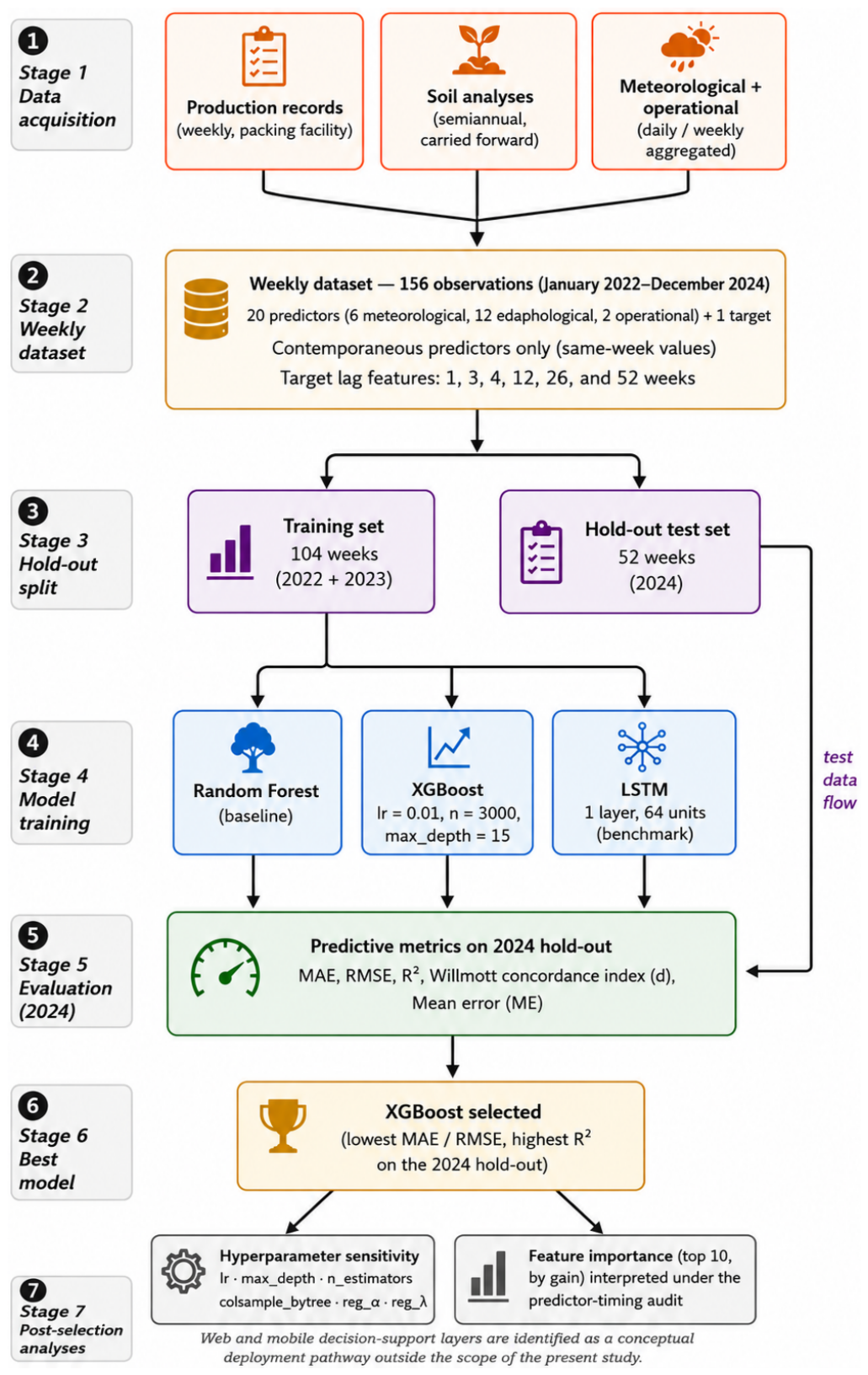
Figure 1 summarizes the methodological workflow for weekly banana production modeling. Production records, semiannual soil analyses, and meteorological and operational data were consolidated into a weekly dataset with 20 original predictor variables and one target variable. In accordance with the predictor-timing audit (

Table 1. Predictor-timing summary. For each input domain, the table indicates the original sampling frequency, whether the same-week value is included in the predictor set, and whether target-derived autoregressive features were applied. Autoregressive features were applied only to the target variable; meteorological, edaphological and operational predictors were included in the model with their contemporaneous (same-week) values.

Variable/Domain	Sampling Frequency	Same-Week	Target-Derived Autoregressive Features
Meteorological predictors (6 variables)	Daily, aggregated weekly	Yes	None
Edaphological predictors (12 variables)	Semiannual laboratory analyses, carried forward	Yes (most recent sample)	None
Bagged bunches (enfundes)	Recorded weekly at bagging time	Yes	None
Harvested bunches	Recorded after weekly harvest is completed	Yes (nowcasting)	None
Calendar/categorical helpers (year, month, week-of-year, bagging color)	Recorded weekly	Yes	None
Processed banana boxes (target, used as autoregressive source)	Recorded at the packing facility after the week ends	Not used directly	1-, 3-, 4-, 12-, 26- and 52-week lags; 4- and 12-week rolling mean and SD (shifted 1 week); 4- and 52-week differences; log of 1-week lag

), meteorological, edaphological, and operational predictors were included in the model with contemporaneous same-week values, whereas lag-engineered features were applied only to the target variable at 1, 3, 4, 12, 26 and 52 weeks. The workflow then proceeds through the chronological hold-out split, model training, evaluation on the 2024 hold-out set, XGBoost selection, and post-selection analyses of hyperparameter sensitivity and feature importance. Web and mobile decision-support layers are identified only as a conceptual deployment pathway outside the scope of the present empirical evaluation [29].

2.1. Experimental Design

The study followed a two-stage experimental design. In the first stage, three representative ML algorithms (Random Forest, XGBoost and LSTM) were compared on the same chronological hold-out partition to compare their predictive performance under the available data conditions. In the second stage, the selected model was profiled with a joint hyperparameter grid search under TimeSeriesSplit cross-validation and re-evaluated on the same 52-week 2024 hold-out with additional metrics (Willmott concordance index and mean error). This procedure distinguishes goodness-of-fit from genuine out-of-sample predictive capacity, a distinction that is especially important in agricultural production modeling where seasonal structure may favor over-fitted models [8].

The comparison was conducted with a stringent chronological split rather than random cross-validation. Models were trained on historical observations and evaluated on temporally subsequent data, thereby reproducing a chronological evaluation scenario and preventing information leakage. This temporal split was selected to provide a more realistic evaluation under operational conditions; we do not claim, however, that this design empirically demonstrates improved external validity for time-series agricultural applications beyond the analyzed farm and study period.

2.2. Study Site and Dataset

Weekly production data were collected at a single commercial banana farm located in Naranjal canton, Guayas Province, Ecuador (approximately 2°${40}^{\prime }$ S, 79°${37}^{\prime }$ W), between January 2022 and December 2024. Data were obtained directly from the operational records of the farm and the associated packing facility under commercial field conditions, rather than from public databases or controlled experiments. The cultivated material corresponded to Williams, a commercial clone within the Cavendish subgroup (AAA), managed under traditional commercial practices for export-oriented banana production in the study area. The plantation was established at a spacing of 3 m × 3 m, equivalent to approximately 1111 plants ${\mathrm{ha}}^{-1}$, assuming one plant per planting site. Because banana production is continuous and staggered under commercial field conditions, plants at different phenological stages coexisted within the same farm during the study period, including vegetative growth, bunch emergence, bagging, fruit filling, and harvesting. The weekly records therefore represent an operational production system rather than a single synchronized experimental phenological stage. The dataset includes twenty predictor variables and one target variable, organized into three domains:

• Meteorological predictors (six variables): mean temperature (°C), total weekly precipitation (mm), mean relative humidity (%), mean wind speed (km/h), dominant wind direction (categorical: Noroeste, Oeste, Sur, Sureste, Suroeste), and mean solar radiation (W/${\mathrm{m}}^2$).
• Edaphological predictors (12 variables): soil pH and concentrations of ${\mathrm{NH}}_4^{+}$, P, K, Ca, Mg, S, Zn, Cu, Fe, Mn, and B. Soil nutrient concentrations were obtained from periodic laboratory analyses conducted every six months. For each 5-ha sampling unit, one composite soil sample was prepared from 10 subsamples, providing a representative estimate of soil chemical conditions at the production-unit scale. The semiannual laboratory values were aligned with the weekly production records by carrying the most recent soil analysis forward until the next sampling date. This procedure allowed the edaphological information to be incorporated into the weekly modeling dataset while recognizing that short-term within-semester nutrient fluctuations were not directly measured.
• Operational predictors (two variables): the number of bagged bunches (enfundes) and the number of harvested bunches. Calendar identifiers (year, month, week-of-year) and the categorical bagging-color code (color de enfunde) were additionally retained in the feature matrix as auxiliary variables; categorical fields were converted to dummy variables via one-hot encoding before model fitting.
• Target variable (one variable): the number of banana boxes processed each week, registered at the packing facility once the week has been completed.

The target variable corresponds to the weekly number of processed banana boxes, that is, the operational production volume registered at the packing facility, and not to the yield expressed per hectare or per plant. In this study, the model outcome is therefore defined as weekly processed-box production rather than agronomic yield. To capture the temporal structure of weekly production, autoregressive features were derived from the target variable: 1-, 3-, 4-, 12-, 26- and 52-week lags; 4- and 12-week rolling means and standard deviations, shifted by one week to avoid leakage; year-over-year (52-week) and month-over-month (four-week) differences; and the natural logarithm of the one-week lag of the target. Lag features were applied only to the target variable; the meteorological, edaphological and operational predictors entered the model with their contemporaneous (same-week) values.

To make the predictive task auditable, Table 1 summarizes the moment at which each input variable becomes available with respect to the target week. For each domain, the table reports the original sampling frequency, whether the same-week value is used, whether lagged values are used, and the availability of the variable relative to the target week.

The variable “harvested bunches” deserves a specific clarification. In its current-week form, this variable becomes available only once the weekly harvest activity has taken place and therefore behaves as a near-term operational proxy of production rather than as a forward-looking agronomic predictor. In the present implementation, it was retained at its contemporaneous (same-week) value because it consistently appeared as a highly informative feature; when used in this form, the resulting model should be interpreted as a same-week explanatory or nowcasting tool rather than as a multi-step-ahead forecasting model. A complementary analysis using only lagged versions of this variable, and excluding the contemporaneous value, is identified as a future-work robustness check.

The practical decision window of the proposed model is the same-week operational estimation. The model estimates the weekly number of processed banana boxes for the week represented by the contemporaneous meteorological, edaphological and operational predictors, combined with autoregressive features derived from past target values (Table 1). Because harvested bunches are included as a same-week predictor, the model can support packing-house planning, short-term logistics adjustment, and production accounting, but it should not be interpreted as a pre-harvest or multi-week-ahead forecasting system. Multi-step-ahead forecasting using lagged-only predictors is identified as an extension for future work.

The full dataset comprised $n=156$ weekly records from 2022 to 2024 (52 observations per year). Data were partitioned chronologically on a calendar-year basis: the 104 weekly records from 2022 and 2023 were used for model training and hyperparameter selection, and the 52 weekly records from 2024 were retained as the unseen final test set. The split is strictly temporal, with no random shuffling and no future information used in the construction of the training features. For the autoregressive lag features that look back beyond the start of 2022 (notably the 52-week lag and the year-over-year difference), the corresponding early-2022 missing values were not removed; they were imputed within the training partition only, as described below.

Data preprocessing followed a single pipeline implemented with scikit-learn’s ColumnTransformer. For the numeric features, including the autoregressive lag features with missing values in early-2022 rows, missing values were imputed with IterativeImputer using max_iter = 10, initial_strategy = "median" and random_state = 42. The imputer was fitted exclusively on the training partition. The parameter n_nearest_features was not restricted, so all available numeric features were considered by the imputation procedure. Categorical features (month name, dominant wind direction and bagging color) were imputed with the most-frequent value and subsequently transformed by one-hot encoding (OneHotEncoder with handle_unknown="ignore"). No explicit outlier filtering or winsorization step was applied. Feature scaling was not used for the tree-based models (Random Forest and XGBoost), which are invariant to monotonic transformations of the input features; the LSTM model received the same numeric features standardized to zero mean and unit variance using statistics estimated only on the training partition.

2.3. Evaluated Models

Three algorithm families were evaluated:

Random Forest (RF) builds an ensemble of decision trees using bootstrap aggregation and feature randomization, reducing overfitting while accommodating mixed-type predictor variables [9]. It serves as a well-established baseline for tabular regression tasks.

Extreme Gradient Boosting (XGBoost) sequentially corrects the residual errors of preceding weak learners using a regularized gradient boosting framework [30]; the original formulation of the algorithm is described in Chen and Guestrin [31]. It was selected for its established performance on tabular data with heterogeneous variables and its interpretability via feature importance scores.

Long Short-Term Memory (LSTM) is a recurrent neural network architecture designed to learn long-range temporal dependencies in sequential data [10], originally introduced by Hochreiter and Schmidhuber [32]. It was included as a benchmark to assess whether explicitly modeling the temporal order of the weekly observations would provide an advantage over tabular methods on this dataset, rather than as an a priori superior approach for short tabular agricultural series.

LSTM Architecture and Training Configuration

The LSTM network was implemented with a recurrent layer followed by a fully connected dense layer with a linear activation function for regression output. An input sequence length of eight steps was used. The model was trained using the Adam optimizer with an initial learning rate of $1\times {10}^{-3}$ and a mean squared error (MSE) loss function. Training was conducted for a maximum of 100 epochs with a batch size of 16, using early stopping with a patience of 10 epochs based on validation loss to prevent overfitting. The validation subset used for early stopping was defined as the most recent contiguous 20% of the training records (chronologically the last weeks before the test split), so that no test-set information was used to determine the stopping epoch. All input features were normalized to zero mean and unit variance using statistics estimated only on the training portion before being passed to the network. A limited LSTM architecture sweep was executed to verify whether the recurrent model underperformance was caused by a single arbitrary configuration. Six configurations around the baseline architecture were evaluated under the same training and 2024 hold-out protocol, varying the number of units, the number of recurrent layers and dropout. The best LSTM configuration (one layer, 64 units, dropout 0.2) yielded MAE = 1081.0 boxes and $R^2=0.13$ on the 2024 hold-out. Although this improved the baseline LSTM result, it remained below the tree-based models, indicating that the LSTM disadvantage was not only an artifact of the initial architecture but also reflected the limited length and tabular structure of the available weekly series.

2.4. Model Evaluation Metrics

Model performance was assessed using three complementary metrics:

$$R^2=1-{\displaystyle \frac{{\sum }_{i=1}^n{(y_i-{\widehat{y}}_i)}^2}{{\sum }_{i=1}^n{(y_i-\overline{y})}^2}}$$

(1)

$$\mathrm{MAE}={\displaystyle \frac{1}{n}}{\displaystyle \sum _{i=1}^n}|y_i-{\widehat{y}}_i|$$

(2)

$$\mathrm{RMSE}=\sqrt{{\displaystyle \frac{1}{n}}\sum _{i=1}^n{(y_i-{\widehat{y}}_i)}^2}.$$

(3)

The Willmott concordance index (d) [3] was additionally computed during the calibration–validation stage:

$$d=1-{\displaystyle \frac{{\sum }_{i=1}^n{(y_i-{\widehat{y}}_i)}^2}{{\sum }_{i=1}^n\left(\right|{\widehat{y}}_i-\overline{y}|+|y_i-\overline{y}{\left|\right)}^2}},$$

(4)

where $y_i$ are observed values, ${\widehat{y}}_i$ are predicted values, and $\overline{y}$ is the observed mean. In all the equations, $y_i$ denotes the observed weekly number of processed banana boxes and ${\widehat{y}}_i$ denotes the corresponding model prediction. The final metrics on the 2024 hold-out are reported as point estimates with bootstrap 95% confidence intervals computed from 2000 resamples of observed–predicted pairs. Hyperparameter selection was performed inside the 2022–2023 calibration partition using GridSearchCV with TimeSeriesSplit; the 2024 hold-out was not used during model selection. The stationarity of the weekly target series was assessed using Augmented Dickey–Fuller (ADF) and KPSS tests. The ADF test rejected the unit-root null ($p=0.0066$), while the KPSS test did not reject the stationarity null ($p>0.10$). Taken together, both tests supported treating the weekly target series as stationary for the purposes of the present modeling workflow.

2.5. Calibration and Hold-Out Evaluation of XGBoost

Because XGBoost achieved the lowest point-error estimates among the evaluated models, it was further calibrated and evaluated under a calendar-year chronological hold-out implemented on the full 156-record dataset. Two temporally separated partitions were used:

• Calibration partition: the 104 weekly records of 2022 and 2023, used exclusively for training and hyperparameter selection of the final XGBoost model.
• Hold-out test partition: the 52 weekly records of 2024, kept aside as a chronological test period used for model comparison and final reporting.

This calendar-year split exposed the model to a full annual cycle of climatic and operational variability that did not contribute to model fitting. The 2024 partition should be interpreted as a chronological hold-out test period for the studied farm, not as a fully external validation dataset. The metrics reported in

Table 2. Predictive performance of Random Forest, XGBoost, and the baseline LSTM on the 2024 hold-out test set (52 weeks). Values are point estimates obtained from the hold-out set, together with bootstrap 95% confidence intervals (in brackets; 2000 resamples). The best LSTM architecture-sweep result is reported in the text because full uncertainty intervals were computed for the baseline comparison table.

Model	MAE (Boxes)	RMSE (Boxes)	${\mathit{R}}^2$
Random Forest	747.55 [616.6, 885.9]	896.68 [756.2, 1032.1]	0.678 [0.473, 0.794]
XGBoost	712.56 [580.2, 855.2]	862.85 [719.8, 997.9]	0.702 [0.522, 0.805]
LSTM (baseline)	1202.66 [919.5, 1515.4]	1638.38 [1266.2, 1978.9]	−0.075 [−0.579, 0.261]

and

Table 3. XGBoost performance on the 2024 hold-out test set (52 weeks), with the model trained on the 104 weekly records of 2022 and 2023. Values are point estimates with bootstrap 95% confidence intervals (2000 resamples) in brackets.

Metric	Symbol	Value [95% CI]
Coefficient of Determination	$R^2$	0.702 [0.522, 0.805]
Willmott Concordance Index	d	0.910 [0.861, 0.941]
Mean Absolute Error	MAE	712.56 boxes [580.2, 855.2]
Root Mean Square Error	RMSE	862.85 boxes [719.8, 997.9]
Mean Error (Bias)	ME	+495.72 boxes [309.4, 689.9]

reflect predictive performance on this 52-week 2024 hold-out set, while the hyperparameter search was conducted inside the calibration partition using TimeSeriesSplit, which preserves temporal ordering during model selection [8].

2.6. Hyperparameter Sensitivity Analysis

Hyperparameter selection for the XGBoost model was performed by joint grid search using GridSearchCV with a time-series-aware cross-validation scheme implemented via TimeSeriesSplit with n_splits = 2. The grid was scored against four metrics in parallel ($R^2$, negative MAE, negative RMSE and negative MAPE), with refitting to the best configuration under the negative MAE criterion. The search ran exclusively on the 104-record calibration partition (2022 and 2023); the 52-record 2024 hold-out test set was held out throughout. The ranges evaluated were:

• learning_rate  $\left(\eta \right)\in \{0.1,0.01,0.005,0.001\}$
• max_depth  $\in \{3,5,7,10,15\}$
• n_estimators  $\in \{100,500,2000,3000\}$
• colsample_bytree  $\in \{0.1,0.5,0.8,1\}$
• reg_alpha  $\in \{1,5,10,20\}$
• reg_lambda  $\in \{1,5,10,20\}$

The optimal XGBoost configuration within the tested ranges was learning_rate $=0.01$, max_depth $=15$, n_estimators $=3000$, colsample_bytree $=1$, reg_alpha $=5$ and reg_lambda $=1$, retained for all subsequent runs. The implementation used Python (v3.13) with xgboost (v3.0.5) and scikit-learn (v1.7.1); importance_type was set to gain, and a fixed random state (42) was used throughout to ensure reproducibility. The 52-week hold-out partition was used only once, to obtain the metrics reported in Table 2 and Table 3. Bootstrap 95% confidence intervals on the 2024 hold-out test predictions were computed by resampling 2000 times the observed–predicted pairs and are reported alongside the point estimates in the next section. The bootstrap 95% confidence intervals of MAE and RMSE across the evaluated n_estimators values are reported in the Results section [33].

3. Results

3.1. Algorithm Comparison on the 2024 Hold-Out Test Set

Table 2 shows the error metrics for the three models on the held-out 2024 data.

XGBoost returned the lowest error on the three metrics ($R^2=0.702$, MAE = 712.56 boxes, RMSE = 862.85 boxes), closely followed by Random Forest ($R^2=0.678$, MAE = 747.55, RMSE = 896.68). The bootstrap 95% confidence intervals of the two tree-based models overlap substantially. Diebold–Mariano paired tests on the absolute-error series of the three baseline-comparison models in Table 2 (small-sample Harvey correction, $h=1$) confirmed that XGBoost and Random Forest were not statistically distinguishable on the 2024 hold-out set ($DM=-1.05$, $p=0.299$), whereas both tree-based models performed significantly better than the LSTM (XGBoost vs. LSTM: $DM=-2.87$, $p=0.006$; Random Forest vs. LSTM: $DM=-2.59$, $p=0.012$). The baseline LSTM result ($R^2=-0.075$) indicates predictive performance close to or below the training-set mean baseline. The subsequent LSTM architecture sweep improved the best recurrent configuration to MAE = 1081.0 boxes and $R^2=0.13$, but it still remained below the performance of Random Forest and XGBoost.

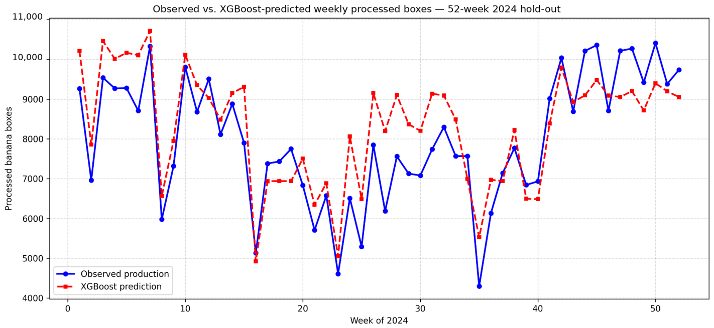
Figure 2 shows the week-by-week comparison between observed and XGBoost-predicted box counts across the 52-week 2024 hold-out set. The model tracks the broad seasonal pattern of weekly production and captures most of the short-term variation, with the largest overshoots concentrated around the Q3 production peak: the three largest positive residuals correspond to weeks 25, 29 and 30 of 2024 (overshoots of approximately +1773, +1818 and +1645 boxes, respectively).

3.2. XGBoost Hyperparameter Sensitivity and Validation

3.2.1. Learning Rate

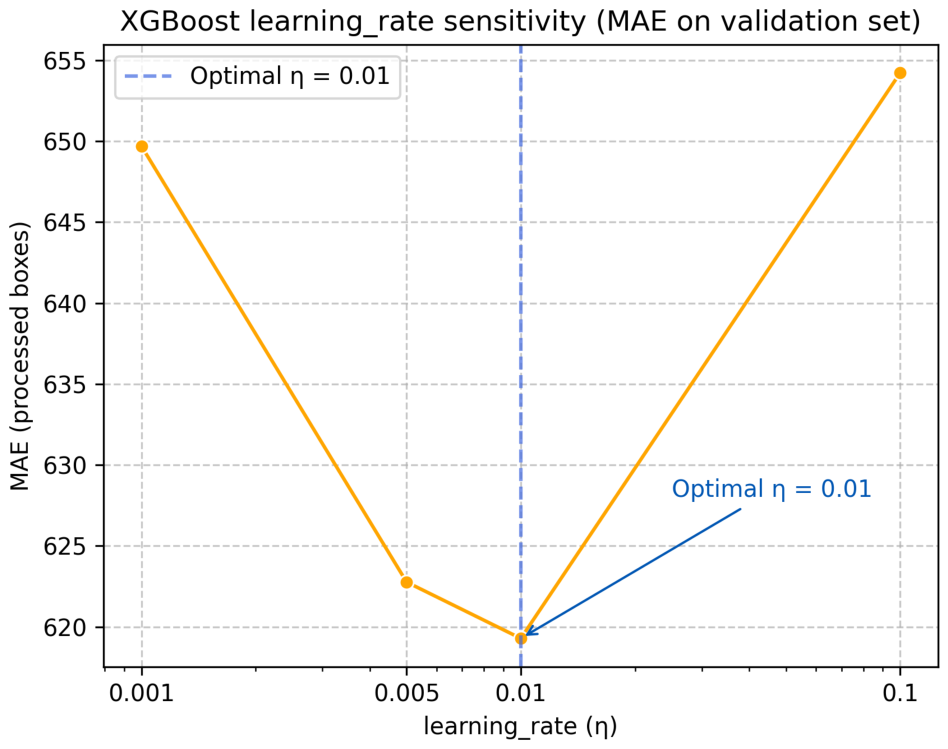
Figure 3 reports the cross-validated MAE for learning rates of 0.001, 0.005, 0.01 and 0.1. Each value was obtained with GridSearchCV, while the remaining hyperparameters were fixed at their joint-search optima: max_depth $=15$, n_estimators $=3000$, colsample_bytree $=1$, reg_alpha $=5$ and reg_lambda $=1$. The lowest cross-validated MAE occurred at $\eta =0.01$, which was retained as the final value.

3.2.2. Number of Trees

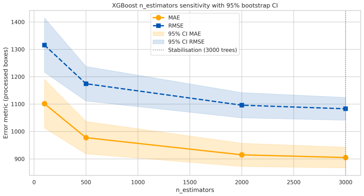
Figure 4 tracks MAE and RMSE as n_estimators grows across the evaluated values $\{100,500,2000,3000\}$. Each point shows the error metric obtained for the corresponding n_estimators value, while the shaded bands report bootstrap 95% confidence intervals. Both metrics decrease as the number of trees increases, with the lowest error observed at 3000 trees, the value retained for the final configuration. The chosen setting should be interpreted as the best-performing configuration within the tested range, not as a general optimum for similar problems.

3.2.3. Feature Importance

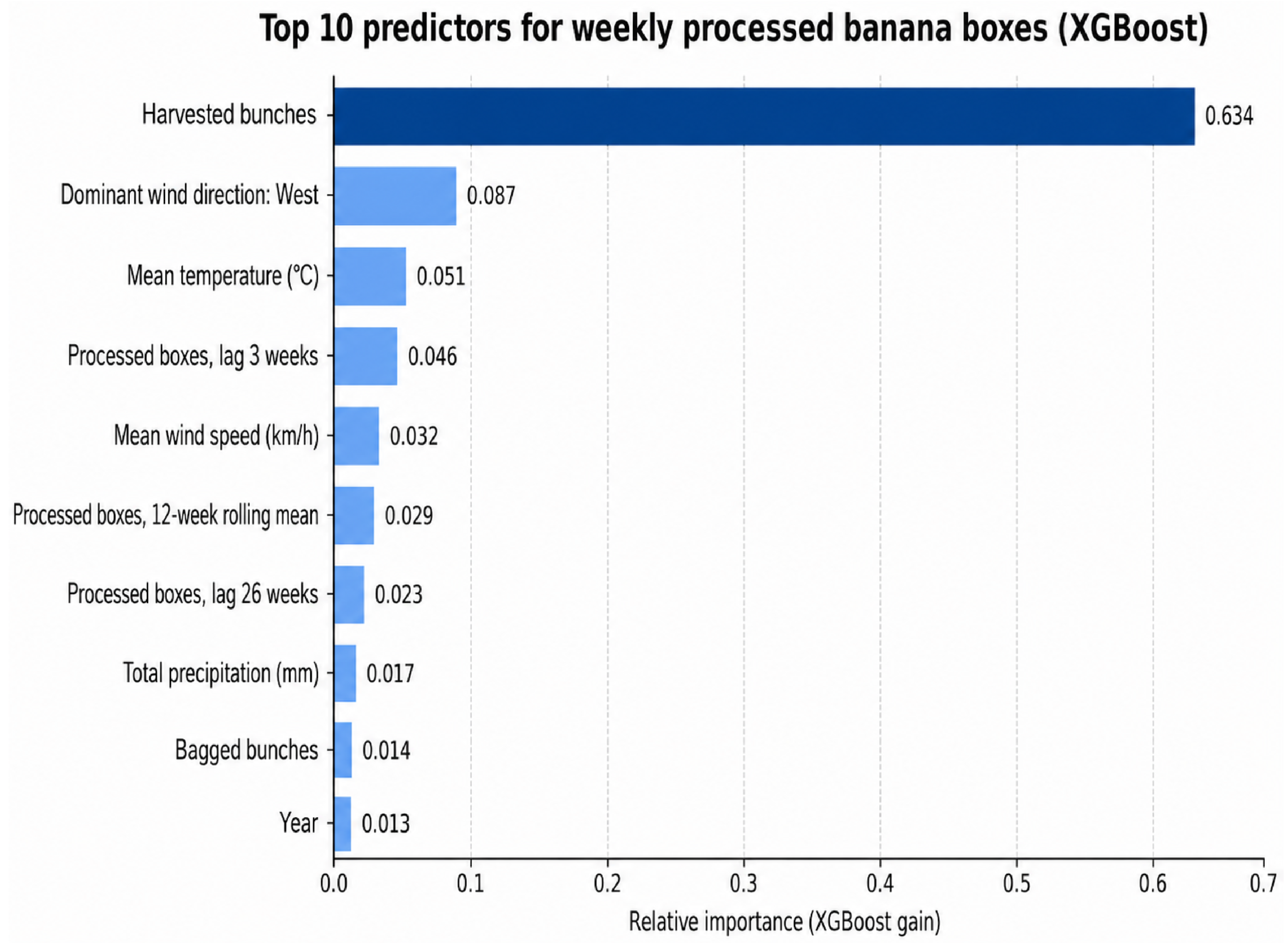
Figure 5 ranks the ten variables with the highest XGBoost gain on the final configuration. The values shown in the figure are: harvested bunches (0.634), dominant wind direction from the west (0.087), mean temperature (0.051), processed boxes lagged by 3 weeks (0.046), mean wind speed (0.032), the 12-week rolling mean of processed boxes (0.029), processed boxes lagged by 26 weeks (0.023), total precipitation (0.017), bagged bunches (0.014) and year (0.013). This ranking indicates that the final XGBoost model combines the same-week operational information, autoregressive production history, weather conditions and seasonal signals. The dominance of harvested bunches confirms its operational proximity to the weekly packing output and reinforces the interpretation of the model as a same-week estimation or nowcasting tool rather than as a strict ahead-of-time forecasting system. Model-agnostic SHAP values computed on the 2024 hold-out partition also identified harvested bunches as the dominant contributor, supporting the interpretation obtained from gain-based importance [26]. The Python code required to compute SHAP values and reproduce the feature-importance workflow is provided in the Supplementary Materials.

3.2.4. Hold-Out Validation of the Final XGBoost Model

Table 3 expands the XGBoost row of Table 2 with the Willmott concordance index (d) and the mean error (ME) on the same 2024 hold-out. The model was trained on the 104-record calibration partition (2022 and 2023), and the metrics were computed once on the 52 weeks of 2024.

Trained on the 104-record calibration partition, the XGBoost model explained 70.2% of the variance of the weekly number of processed boxes on the 2024 hold-out. The Willmott concordance index ($d=0.910$) indicates that the predicted series tracks the observed one closely in both timing and magnitude. Following the convention implemented in the source code, $\mathrm{ME}=\overline{\widehat{y}}-\overline{y}$, so the positive value of $+495.72$ boxes per week corresponds to an average overestimation of approximately 6.8% of the mean weekly volume on the test segment, with the bootstrap 95% confidence interval strictly above zero. This systematic deviation is consistent with the residual pattern in Figure 2, where the model overshoots at the Q3 production peak (weeks 25, 29 and 30 of 2024). Plausible explanations, not tested in the present study, include unobserved operational decisions (for example, irrigation scheduling, fungicide applications) and early-stage production losses that the predictor set cannot capture.

4. Discussion

XGBoost achieved the best numerical performance on the 52-week 2024 hold-out, followed closely by Random Forest, with no statistically significant difference between the two tree-based models according to the Diebold–Mariano test. LSTM showed weaker predictive performance under the available data conditions. The extended evaluation of the final XGBoost model added the Willmott concordance index and mean error on the same 2024 hold-out (Table 3). This result is consistent with previous reports by Patrick et al. [8] and Salman et al. [9], where tree-based models perform competitively on tabular agricultural datasets.

The LSTM result requires a careful interpretation. The baseline recurrent network produced weak performance on the 2024 hold-out, and the architecture sweep improved the best recurrent configuration to MAE = 1081.0 boxes and $R^2=0.13$, but did not close the gap with the tree-based models. This finding suggests that the underperformance of the LSTM was not merely a consequence of one arbitrary architecture. One plausible explanation is the mismatch between the inductive bias of LSTM networks [32] and the structure of the available data. Recurrent architectures gain most when the sequential order of inputs carries information that concurrent variables do not (speech, text, or sensor streams measured at sub-second resolution are good examples). Weekly agricultural records are different. The agronomic state of the plantation at week t is encoded in the simultaneous values of soil nutrients, recent rainfall, and bunch counts at that same week; the additional signal from earlier weeks, once autoregressive target features are included in the tabular models, appears small. This observation does not rule out recurrent models for banana production estimation in general; it indicates that, on this dataset and under the tested LSTM configurations, the recurrent approach did not provide an advantage. Longer time series, richer within-week sensor data or attention-based sequence models could yield different results [34].

The feature-importance ranking has an operational and agronomic interpretation. The dominance of harvested bunches indicates that the model relies strongly on the same-week production availability. This result is coherent from an operational perspective because the number of harvested bunches is directly linked to the volume of fruit entering the packing facility. However, it also limits the forecasting interpretation of the model: when contemporaneous harvested bunches are included, the model supports same-week production estimation or nowcasting rather than multi-week-ahead forecasting. The 3-week and 26-week lags of processed boxes and the 12-week rolling mean of processed boxes show that recent and seasonal production history contributed to the prediction. Dominant wind direction from the west, mean temperature, mean wind speed, and total precipitation provide weather-related signals, while bagged bunches and the year variable represent operational and calendar information. These associations are agronomically plausible, but they should not be interpreted as causal effects. The study is observational, and XGBoost feature importance measures contribution to predictive accuracy rather than causal influence.

Compared with regional studies from Tanzania [8] and from Africa and Asia more broadly [2], this work operates at finer spatial and temporal resolution by analyzing weekly records from a single commercial farm and by using a calendar-year chronological hold-out design with time-series-aware cross-validation inside the hyperparameter search. This design reduces the risk of leakage-driven inflation relative to randomly shuffled validation schemes, although the results remain conditional on one farm and a limited number of production years. The positive mean error (ME $=+495.72$ boxes per week, with a bootstrap 95% confidence interval of [309.4, 689.9], approximately 6.8% of the mean weekly volume on the test segment) corresponds to systematic overestimation of the weekly volume. Several candidate hypotheses, not tested in the present study, could account for this deviation, including unobserved operational decisions such as irrigation scheduling or targeted fungicide applications, as well as phytosanitary pressure not represented in the predictor set. The ADF and KPSS tests jointly supported treating the weekly target series as stationary for the purposes of the present modeling workflow. Same-week production estimates of this type could support harvest logistics and packing-station scheduling at the studied farm; broader use in monitoring or decision-support systems would require additional multi-farm validation and is identified as future work [35].

Limitations

The results should be interpreted against several constraints. All 156 weekly records come from a single farm in Naranjal canton, and the dataset corresponds to a small sample size by current machine learning standards. Hyperparameter selection used time-series cross-validation through TimeSeriesSplit with two folds within GridSearchCV; the final predictive metrics on the 52-week 2024 hold-out are accompanied by 95% bootstrap confidence intervals (Table 2 and Table 3). The Diebold–Mariano paired tests were executed on the 2024 hold-out absolute-error series of the three baseline-comparison models in Table 2 and showed that the numerical difference between XGBoost and Random Forest was not statistically significant ($DM=-1.05$, $p=0.299$), whereas both tree-based models were significantly better than the LSTM (XGBoost vs. LSTM: $DM=-2.87$, $p=0.006$; Random Forest vs. LSTM: $DM=-2.59$, $p=0.012$). Thus, XGBoost should be described as the best numerical model in this dataset, not as categorically superior to Random Forest. Rerunning the grid search with more time-series folds remains a robustness refinement for future work. Soil variability, microclimate differences, and local management practices across Ecuador’s main banana zones mean the model would need recalibration before being applied elsewhere; transferability has not been evaluated. The three-year window (2022–2024) captures a narrow slice of climatic variability. A severe El Niño year or an exceptional drought falling outside this range could expose gaps in the model’s learned structure that are invisible in the current evaluation.

The predictor set has no direct measure of plant health, disease incidence, or irrigation input. These are not minor omissions. Disease pressure can suppress bunch development for weeks before it shows up in production counts, and its absence from the feature set may contribute to the systematic overestimation observed on the 2024 hold-out. The LSTM architecture sweep was executed and showed that the best tested recurrent configuration improved the baseline LSTM result, but did not reach the performance level of the tree-based models. Therefore, the LSTM finding should be interpreted as an empirical result for the tested configurations and data conditions, not as general evidence against recurrent models in banana production estimation. Finally, soil measurements were taken at fixed sampling intervals; whether those intervals matched actual nutrient dynamics, or whether some readings were noisy or interpolated, was not assessed. Measurement error in the edaphological variables could distort the feature importance estimates. In addition, the contemporaneous use of harvested bunches as a predictor implies that part of the predictive performance reflects same-week operational information; further analysis using only lagged versions of this variable is recommended to better characterize its contribution under a strict ahead-of-time forecasting setting (see Table 1).

5. Conclusions

Within the data conditions and farm scope analyzed, XGBoost explained 70.2% of the variability of the weekly number of processed banana boxes on the 52-week 2024 hold-out set ($d=0.910$; MAE = 712.56 boxes; bootstrap 95% confidence interval for $R^2$: [0.522, 0.805]), trained on the 104 weekly records from 2022 and 2023. This performance, obtained on a dataset that remains small for machine learning standards, suggests that gradient boosting can support weekly production planning at the studied farm during the study period. These findings should not be extended to all banana plantations in Ecuador, to similar regions or to banana production in general without additional multi-farm and multi-season validation.

The three-algorithm comparison produced a proportionate ranking on the analyzed dataset: XGBoost achieved the best numerical performance, Random Forest followed closely with statistically indistinguishable error under the Diebold–Mariano test, and LSTM showed weaker predictive performance even after the limited architecture sweep. Within this dataset, the concurrent state of soil, weather and operational predictors, together with autoregressive target features, carried more useful predictive information than the tested recurrent sequence structures. Recurrent models could still be advantageous on banana datasets with longer series, finer temporal resolution or richer sensor information, so the comparative conclusion remains limited to the available evidence.

The top predictors under the final configuration were harvested bunches, dominant wind direction from the west, mean temperature, the 3-week lag of processed boxes, mean wind speed, the 12-week rolling mean of processed boxes, the 26-week lag of processed boxes, total precipitation, bagged bunches and year. These features are operationally and agronomically interpretable, although the model is observational, and feature importance does not establish causal relationships. Because contemporaneously harvested bunches become available only after the weekly harvest operation, the current model is best interpreted as a same-week production estimation or nowcasting tool. A strict ahead-of-time forecasting model should be evaluated using lagged-only operational predictors and additional agronomic, phytosanitary and irrigation variables. Thus, the practical contribution of the current model lies in operational same-week estimation, whereas strict ahead-of-time forecasting remains a separate modeling task.

On the methodological side, the sensitivity analysis indicated that, within the tested ranges, the lowest predictive error was obtained with a learning rate of 0.01, 3000 trees, and a maximum tree depth of 15. These values are dataset-specific and should not be interpreted as general optima for similar problems. Computational cost scales with the number of trees, which is a relevant practical consideration for deployments that must run weekly on farm hardware or cloud infrastructure with budget constraints. Given the limited sample size, this hyperparameter configuration should be interpreted as the best setting within the tested grid for the present dataset, not as a transferable recommendation for other farms, years or banana production systems.

Three directions stand out for future work. First, extending data collection to multiple farms across Guayas and El Oro provinces and incorporating additional production seasons would allow a proper test of whether a single model can transfer across sites or whether site-specific recalibration is required. Second, adding plant-health indicators (for example, disease incidence scores or canopy reflectance from low-cost sensors) would directly address the systematic deviation observed on the 2024 hold-out. Third, the Fusarium TR4 risk documented in Ecuadorian plantations [36] reinforces the need for production-estimation models that integrate phytosanitary signals; the architecture developed here is identified as a candidate starting point for that extension. Future work should prioritize external multi-farm validation, stricter ahead-of-time forecasting with lagged-only predictors, additional time-series cross-validation folds, richer sequence models under larger datasets and the integration of plant-health, irrigation and disease-pressure indicators.

References

1. Vaca, E.; Gaibor, N.; Kovács, K. Analysis of the chain of the banana industry of Ecuador and the European market. APSTRACT Appl. Stud. Agribus. Commer. 2020, 14, 55–64. [Google Scholar] [CrossRef]
2. Olivares, B.O.; Vega, A.; Rueda Calderón, M.A.; Montenegro-Gracia, E.; Araya-Almán, M.; Marys, E. Prediction of banana production using epidemiological parameters of black Sigatoka: An application with Random Forest. Sustainability 2022, 14, 14123. [Google Scholar] [CrossRef]
3. Jayasinghe, S.L.; Ranawana, C.J.K.; Liyanage, I.C.; Kaliyadasa, P.E. Growth and yield estimation of banana through mathematical modelling: A systematic review. J. Agric. Sci. 2022, 160, 152–167. [Google Scholar] [CrossRef]
4. Zubelzu, S.; Panigrahi, N.; Thompson, A.J.; Knox, J.W. Modelling water fluxes to improve banana irrigation scheduling and management in Magdalena, Colombia. Irrig. Sci. 2023, 41, 69–79. [Google Scholar] [CrossRef]
5. Quiloango-Chimarro, C.A.; Gioia, H.R.; De Oliveira Costa, J. Typology of production units for improving banana agronomic management in Ecuador. AgriEngineering 2024, 6, 2811–2823. [Google Scholar] [CrossRef]
6. De Souza, A.V.; Neto, A.B.; Piazentin, J.C.; Junior, B.J.D.; Gomes, E.P.; Bonini, C.d.S.B.; Putti, F.F. Artificial neural network modelling in the prediction of bananas’ harvest. Sci. Hortic. 2019, 257, 108724. [Google Scholar] [CrossRef]
7. Khan, T.; Qiu, J.; Ali Qureshi, M.A.; Iqbal, M.S.; Mehmood, R.; Hussain, W. Agricultural fruit prediction using deep neural networks. Procedia Comput. Sci. 2020, 174, 72–78. [Google Scholar] [CrossRef]
8. Patrick, S.; Mirau, S.; Mbalawata, I.; Leo, J. Time series and ensemble models to forecast banana crop yield in Tanzania, considering the effects of climate change. Resour. Environ. Sustain. 2023, 14, 100138. [Google Scholar] [CrossRef]
9. Salman, H.A.; Kalakech, A.; Steiti, A. Random Forest algorithm overview. Babylon. J. Mach. Learn. 2024, 2024, 69–79. [Google Scholar] [CrossRef]
10. Van Houdt, G.; Mosquera, C.; Nápoles, G. A review on the long short-term memory model. Artif. Intell. Rev. 2020, 53, 5929–5955. [Google Scholar] [CrossRef]
11. Khan, T.; Sherazi, H.H.R.; Ali, M.; Letchmunan, S.; Butt, U.M. Deep learning-based growth prediction system: A use case of China agriculture. Agronomy 2021, 11, 1551. [Google Scholar] [CrossRef]
12. Botero-Valencia, J.; García-Pineda, V.; Valencia-Arias, A. Machine Learning in Sustainable Agriculture: Systematic Review and Research Perspectives. Agriculture 2025, 15, 377. [Google Scholar] [CrossRef]
13. Jarne, A.; Usón, A.; Reiné, R. Assessing the Impact of Environmental and Management Variables on Mountain Meadow Yield and Feed Quality Using a Random Forest Model. Plants 2025, 14, 2150. [Google Scholar] [CrossRef] [PubMed]
14. Singh, K.; Yadav, M.; Barak, D.; Bansal, S.; Moreira, F. Machine-Learning-Based Frameworks for Reliable and Sustainable Crop Forecasting. Sustainability 2025, 17, 4711. [Google Scholar] [CrossRef]
15. Sharma, R. Artificial intelligence in agriculture: A review. In Proceedings of the 5th International Conference on Intelligent Computing and Control Systems (ICICCS), Madurai, India, 6–8 May 2021; pp. 937–942. [Google Scholar] [CrossRef]
16. Olsen, T.L.; Tomlin, B. Industry 4.0: Opportunities and challenges for operations management. Manuf. Serv. Oper. Manag. 2020, 22, 113–122. [Google Scholar] [CrossRef]
17. Celis Crisostomo, M.A.; Hernández López, F.M.; Cárdenas Magaña, J.A.; Vega Negrete, E. Implementación de microservicios en proyectos de IoT con Arduino. INGENIUS 2025, 34, 9–19. [Google Scholar] [CrossRef]
18. Amador-Sacoto, C.; Helfgott-Lerner, S. Sustainability of sugarcane farms in the Milagro Canton, Ecuador. Int. J. Adv. Sci. Eng. Inf. Technol. 2023, 13, 837–843. [Google Scholar] [CrossRef]
19. Herrera-Franco, G.; Sánchez-Arizo, V.; Escandon-Panchana, P.; Caicedo-Potosí, J.; Jaya-Montalvo, M.; Zambrano-Mendoza, J. Analysis of scientific contributions to agricultural development and food security in Ecuador. Int. J. Des. Nat. Ecodyn. 2023, 18, 1129–1139. [Google Scholar] [CrossRef]
20. Luzuriaga-Amador, M.; Novillo-Luzuriaga, N.; Guevara-Viejó, F.; Valenzuela-Cobos, J.D. Evaluation of the performance of information competencies in the fertilization and trade strategies of small banana producers in Ecuador. Sustainability 2025, 17, 868. [Google Scholar] [CrossRef]
21. Abdullah, N.; Mohd Taib, R.; Mohamad Aziz, N.S.; Omar, M.R.; Md Disa, N. Banana pseudo-stem biochar derived from slow and fast pyrolysis process. Heliyon 2023, 9, e12940. [Google Scholar] [CrossRef]
22. Valenzuela-Cobos, J.D.; Pérez-Martínez, S.; Fiallos-Cárdenas, M.; Guevara-Viejó, F. Data mining for the characterization of a paper prototype obtained with bacterial cellulose derived from banana and pineapple by-products. Appl. Sci. 2024, 14, 11426. [Google Scholar] [CrossRef]
23. Hu, J.; Szymczak, S. A review on longitudinal data analysis with Random Forest. Brief. Bioinform. 2023, 24, bbad002. [Google Scholar] [CrossRef]
24. Contreras Urgiles, W.R.; León Japa, R.S.; Maldonado Ortega, J.L. Predicción de emisiones de CO y HC en motores Otto mediante redes neuronales. INGENIUS 2019, 23, 30–39. [Google Scholar] [CrossRef]
25. Kumari, P.; Goswami, V.; Harshith, N.; Pundir, R.S. Recurrent neural network architecture for forecasting banana prices in Gujarat, India. PLoS ONE 2023, 18, e0275702. [Google Scholar] [CrossRef]
26. Nguyen, V.G.; Sharma, P.; Ağbulut, Ü.; Le, H.S.; Cao, D.N.; Dzida, M.; Osman, S.M.; Le, H.C.; Tran, V.D. Improving the prediction of biochar production from various biomass sources through the implementation of eXplainable machine learning approaches. Int. J. Green Energy 2024, 21, 2771–2798. [Google Scholar] [CrossRef]
27. Houngue, J.A.; Houédjissin, S.S.; Ahanhanzo, C.; Pita, J.S.; Houndénoukon, M.S.E.; Zandjanakou-Tachin, M. Cassava mosaic disease (CMD) in Benin: Incidence, severity and whitefly abundance from field surveys in 2020. Crop Prot. 2022, 158, 106007. [Google Scholar] [CrossRef] [PubMed]
28. Mancero-Castillo, D.; Garcia, Y.; Aguirre-Munizaga, M.; Ponce De Leon, D.; Portalanza, D.; Avila-Santamaria, J. Dynamic perspectives into tropical fruit production: A review of modeling techniques. Front. Agron. 2024, 6, 1482893. [Google Scholar] [CrossRef]
29. Cedric, L.S.; Adoni, W.Y.H.; Aworka, R.; Zoueu, J.T.; Mutombo, F.K.; Krichen, M.; Kimpolo, C.L.M. Crops yield prediction based on machine learning models: Case of West African countries. Smart Agric. Technol. 2022, 2, 100049. [Google Scholar] [CrossRef]
30. Ibrahem Ahmed Osman, A.; Najah Ahmed, A.; Chow, M.F.; Feng Huang, Y.; El-Shafie, A. Extreme gradient boosting (XGBoost) model to predict the groundwater levels in Selangor, Malaysia. Ain Shams Eng. J. 2021, 12, 1545–1556. [Google Scholar] [CrossRef]
31. Chen, T.; Guestrin, C. XGBoost: A Scalable Tree Boosting System. In Proceedings of the 22nd ACM SIGKDD International Conference on Knowledge Discovery and Data Mining, New York, NY, USA, 13–17 August 2016; pp. 785–794. [Google Scholar] [CrossRef]
32. Hochreiter, S.; Schmidhuber, J. Long Short-Term Memory. Neural Comput. 1997, 9, 1735–1780. [Google Scholar] [CrossRef]
33. Aguirre-Munizaga, M.; Chang-Zorilla, S.; Rivera, D.V.; Vera-Lucio, N. Implementation of a web application for estimating cocoa productivity using machine learning. In Information Technology and Systems; Lecture Notes in Networks and Systems; Springer Nature: Cham, Switzerland, 2025; Volume 1447, pp. 382–390. [Google Scholar] [CrossRef]
34. Huang, R.; Wei, C.; Wang, B.; Yang, J.; Xu, X.; Wu, S.; Huang, S. Well performance prediction based on Long Short-Term Memory (LSTM) neural network. J. Pet. Sci. Eng. 2022, 208, 109686. [Google Scholar] [CrossRef]
35. Aijaz, N.; Lan, H.; Raza, T.; Yaqub, M.; Iqbal, R.; Pathan, M.S. Artificial intelligence in agriculture: Advancing crop productivity and sustainability. J. Agric. Food Res. 2025, 20, 101762. [Google Scholar] [CrossRef]
36. Fernández-Ledesma, C.M.; Garcés-Fiallos, F.R.; Rosso, F.; Cordero, N.; Ferraz, S.; Durigon, A.; Portalanza, D. Assessing the risk of Fusarium oxysporum f. sp. cubense Tropical Race 4 outbreaks in Ecuadorian banana crops using spatial climatic data. Sci. Agropecu. 2023, 14, 301–312. [Google Scholar] [CrossRef]
Figure 1. Methodological workflow for weekly banana production modeling involved integrating production records, semiannual soil analyses, and meteorological and operational data into a weekly dataset with 20 original predictor variables and one target variable. Meteorological, edaphological, and operational predictors were included in the model with contemporaneous same-week values; lag-engineered features were applied only to the target variable at 1, 3, 4, 12, 26 and 52 weeks. The workflow includes the chronological hold-out split, model training, evaluation on the 2024 hold-out set, XGBoost selection, and post-selection analyses of hyperparameter sensitivity and feature importance.
Agriculture 16 01182 g001
Figure 2. Observed vs. XGBoost-predicted weekly processed boxes—2024 hold-out. The solid blue line represents observed production and the dashed red line represents model predictions. The annotated weeks indicate the largest positive residuals, where the model overestimated the observed weekly volume.
Agriculture 16 01182 g002
Figure 3. Sensitivity of XGBoost predictive error (MAE) to the learning_rate hyperparameter. Values are cross-validated MAE from GridSearchCV with TimeSeriesSplit, holding the remaining hyperparameters at their best-search values. The minimum cross-validated MAE is achieved at η = 0.01 .
Agriculture 16 01182 g003
Figure 4. Sensitivity of XGBoost MAE and RMSE to n_estimators across the evaluated values { 100 , 500 , 2000 , 3000 } . Lines show the evaluated error metrics, and shaded bands represent bootstrap 95% confidence intervals. Within the analyzed dataset, error decreased as the number of trees increased and stabilized near 3000 estimators, the configuration retained for the final model.
Agriculture 16 01182 g004
Figure 5. Top-10 predictor variables ranked by XGBoost feature importance based on relative gain for weekly processed-box estimation. Harvested bunches were the dominant predictor, indicating the strong contribution of same-week operational information to the model. Lagged processed-box variables and the 12-week rolling mean represent historical production features and must be interpreted as autoregressive predictors. Feature-importance values indicate predictive contribution and do not imply causal effects.
Agriculture 16 01182 g005