Accurate Inversion of Rice LAI Using UAV-Based Hyperspectral Data: Integrating Days After Transplanting and Meteorological Factors

Abstract

The leaf area index (LAI) is a key physiological parameter characterizing rice canopy structure and growth status. To face the limits of traditional destructive sampling, which is time-consuming, labor-intensive, and difficult to achieve large-scale dynamic detection, this study proposes a precise UAV-based hyperspectral inversion method for rice LAI using the fusion of Days After Transplantation and Meteorological Factors data (DATaMF). The study framework consisted of three key components: spectral preprocessing (smoothing-R_SG, resampling-R_RS, first derivative transformation-R_FD), spectral feature selection (SPA, CARS, Relief-F), and the construction and assessment of LAI inversion models (RF, ELM, XGBoost) that integrated DATaMF. The results show that (1) the three-level data preprocessing procedure—comprising R_SG, R_RS, and R_FD—coupled with the feature subset selected by the CARS method, demonstrates strong performance in LAI inversion; (2) the incorporation of DATaMF significantly improves rice LAI estimation, leading to improved model accuracy and robustness; and (3) the optimal LAI inversion model is achieved with the RF-based CARS-R_FD-DATaMF approach, yielding test set R², RMSE, and RPD values of 0.8015, 0.5745, and 2.2857, respectively. In conclusion, the hyperspectral LAI inversion method developed in this study, which integrates DATaMF, significantly enhances the model’s accuracy and stability under small-sample conditions. This approach provides reliable technical support for efficient, precise, and dynamic monitoring of rice growth.

1. Introduction

Leaf area index (LAI) is a critical physiological parameter for characterizing rice canopy structure and growth [1], with significant influences on photosynthetic efficiency [2], transpiration rate [3,4], and final yield [5]. Conventional methods for obtaining LAI, including destructive sampling and canopy analyzers, are accurate [6] but limited by their time-consuming and labor-intensive procedures. These drawbacks make them impractical for the large-scale, high-frequency dynamic monitoring required in modern rice production systems.

In recent years, UAV-based hyperspectral remote sensing has emerged as a key technology in modern smart agriculture, owing to its unique capability for rapid, non-destructive, and multi-temporal acquisition of spectral information in the field [7]. In contrast to multispectral data, hyperspectral data provide richer and more continuous spectral characteristics [8], which capture finer details on the physiological, biochemical, and structural properties of the rice canopy. This provides essential data support for the accurate and efficient inversion of rice LAI.

The precise inversion of LAI using UAV remote sensing has evolved through significant paradigm shifts, progressing from empirical statistical models to complex machine learning algorithms, and from broadband vegetation indices to narrowband hyperspectral features [9,10]. Early studies primarily estimated LAI by establishing statistical relationships between the parameter and traditional vegetation indices, such as the Normalized Difference Vegetation Index (NDVI) and the Enhanced Vegetation Index (EVI) [11]. Advances in sensor technology, along with a detailed understanding of the spectral response to crop physiological mechanisms, have gradually shifted the focus of remote sensing toward the refined mining and application of spectral features [12,13]. Studies indicate that the choice of bandwidth is a critical factor, as narrowband, mid-frequency, and broadband vegetation indices yield varying levels of accuracy in LAI inversion [14]. Meanwhile, the rapid development of machine learning algorithms such as Random Forests (RF) and Extreme Learning Machine (ELM) has demonstrated powerful nonlinear modeling capabilities [15], effectively establishing complex nonlinear mapping relationships between spectra and growth and physiological indicator, such as rice LAI, significantly improving the inversion accuracy of the model.

However, several challenges persist in inverting rice LAI using hyperspectral data. First, the stability of the canopy spectrum–LAI relationship can be compromised by complex field conditions, such as variations in soil background and illumination, as well as dynamically changing meteorological factors including temperature, wind speed, and relative humidity [16]. These factors adversely affect the accuracy and robustness of inversion models. Second, the high dimensionality and strong multicollinearity of the original UAV canopy spectral data, combined with a limited sample size, can induce the Hughes phenomenon [17], which reduces the model’s generalization capability, obscures the true spectral–LAI interaction mechanisms, and limits the model’s applicability across different rice varieties and growing environments. Furthermore, given that LAI is a dynamic parameter that evolves throughout the rice growth cycle, the integration of temporal phase information into inversion models becomes a critical consideration.

Therefore, to address the aforementioned challenges, this study proposes a precise UAV-based hyperspectral inversion strategy for rice LAI, driven by the integration of Days After Transplantation and Meteorological Factors (DATaMF) data, providing an effective solution for rice LAI inversion under small-sample conditions. The core contents of this study are as follows: (1) to extract key spectral information related to LAI through systematic spectral preprocessing and feature dimensionality reduction; (2) to investigate the influence of DATaMF incorporation on the inversion performance of different machine learning models; (3) to determine the optimal inversion model for rice LAI under small-sample conditions.

2. Materials and Methods

2.1. Trial Design and Research Area Overview

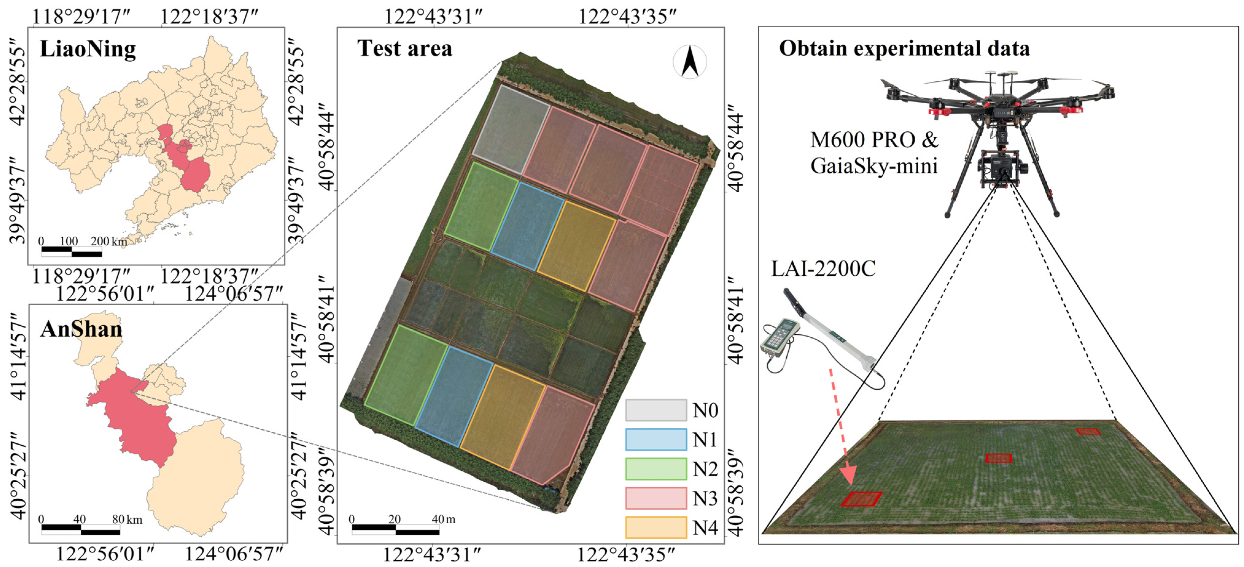
The experiment was conducted from June to September 2023 at the experimental field of the Precision Agriculture Aviation Research Base of Shenyang Agricultural University, Gengzhuang Town, Haicheng City, Anshan City, Liaoning Province, China (40°58′45″ N, 122°43′35″ E). The region is characterized by fertile soil, distinct seasons, and abundant rainfall, providing an ideal environment for rice cultivation. The rice cultivar used was ‘Shennong 9816’ (Shenyang, China). The layout of the experimental field is shown in Figure 1. A total of five nitrogen fertilizer gradients were set, namely, zero nitrogen fertilizer, low nitrogen fertilizer, medium nitrogen fertilizer, standard nitrogen fertilizer, and high nitrogen fertilizer, which were, respectively, recorded as N0, N1, N2, N3, and N4, among which N3 was 220.5 kg/ha. The fertilizer was applied in a base-tillering-panicle ratio of 5:3:2. The application rates for N1, N2, and N4 were set at −50%, −25%, and +25% of N3, respectively. All plots received consistent field management practices. The field sampling period was from the tillering stage to the heading stage of rice, with a sampling interval of 4 days. A total of 141 sets of UAV canopy spectra and corresponding LAI data were collected.

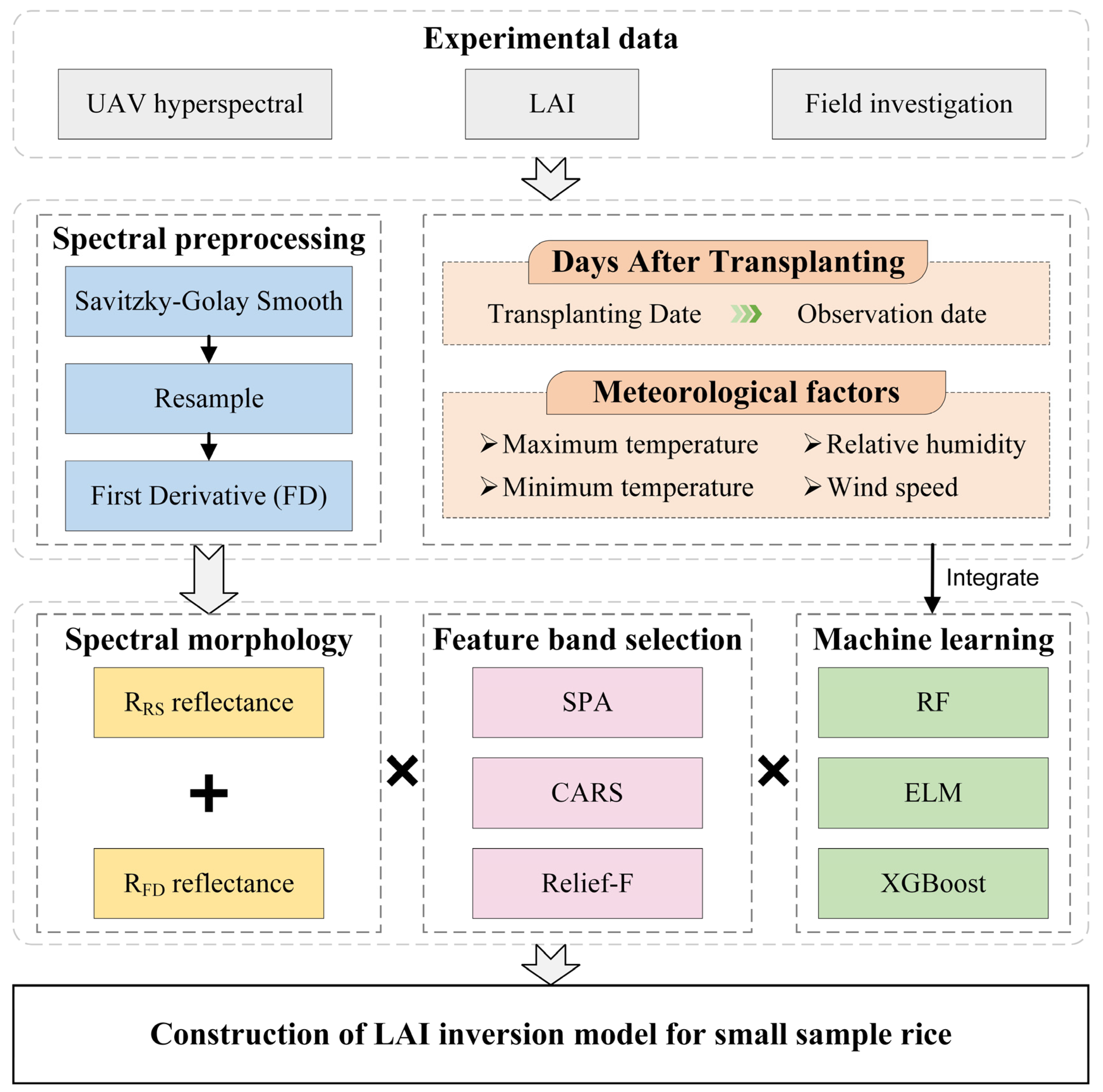
The overall technical route of this study is shown in Figure 2. Firstly, a three-level data preprocessing process, including Savitzky–Golay smooth denoising (R_SG), resampling (R_RS), and First derivative transformation (R_FD), is utilized to process the spectral data (R_UAV) collected by the UAV. The key feature bands in R_RS and R_FD are screened by combining three feature selection methods: Successive Projection Algorithm (SPA), Competitive Adaptive Reweighted Sampling (CARS), and Relevant Features (Relief-F). Meanwhile, DATaMF was introduced to construct the rice LAI inversion model based on three machine learning algorithms: Random Forests (RF), Extreme Learning Machine (ELM), and eXtreme Gradient Boosting (XGBoost), and the performance of the model was systematically evaluated and comparatively analyzed.

2.2. Data Acquisition

2.2.1. Acquisition of UAV-Based Canopy Hyperspectral Data

In this study, the M600 PRO hexacopter UAV from Shenzhen DJI Innovation Co., Ltd. (Shenzhen, China) was used as the remote sensing platform, and at the same time, the GaiaSky-mini built-in push-broom hyperspectral imaging system from Dualix Spectral Imaging Co., Ltd. (Wuxi, China) was equipped to collect the data of hyperspectral images on the canopy of the rice UAV. The UAV was operated at a flight altitude of 100 m. The hyperspectral imager has a spectral resolution of 3.5 nm, covering a range of 400–1000 nm with 170 effective bands. The spatial resolution was 7 cm, with a single image acquisition time of 15 s and a frame rate of 162 fps. All data were acquired between 10:00 and 14:00 local time. Prior to each flight, dark current and whiteboard corrections were performed. At the same time, a 1.5 m × 1.5 m diffuse reflector with a reflectivity of 60% was placed simultaneously in the rice canopy observation area for the correction of reflection data in the later stage. Based on the SpectraVIEW spectral processing software (Dualix Spectral Imaging, Wuxi, China), the collected hyperspectral images were preprocessed for lens, uniformity, reflectance, etc. The ENVI5.3 + IDL tool software (GeoScene Information Technology Co., Beijing, China) was used to extract the spectral reflectance data of the canopy layer of the rice UAV at the sampling points.

2.2.2. Acquisition of Rice Leaf Area Index (LAI) Data

In this study, the LAI-2200C plant canopy analyzer (Li-Cor, Inc., Lincoln, NE, USA) was used to measure the LAI of the rice canopy at ground level. The instrument determines LAI values by measuring radiation above and below the canopy using fisheye lens sensors. To ensure the reliability of the data, three measurement points were established in each test field. At each measurement point, three repeated measurements were carried out strictly in accordance with the instrument operation specifications, and the final average value was taken as the effective LAI value of the sampling area [18].

2.2.3. Acquisition and Organization of Data on Days After Transplantation and Meteorological Factors

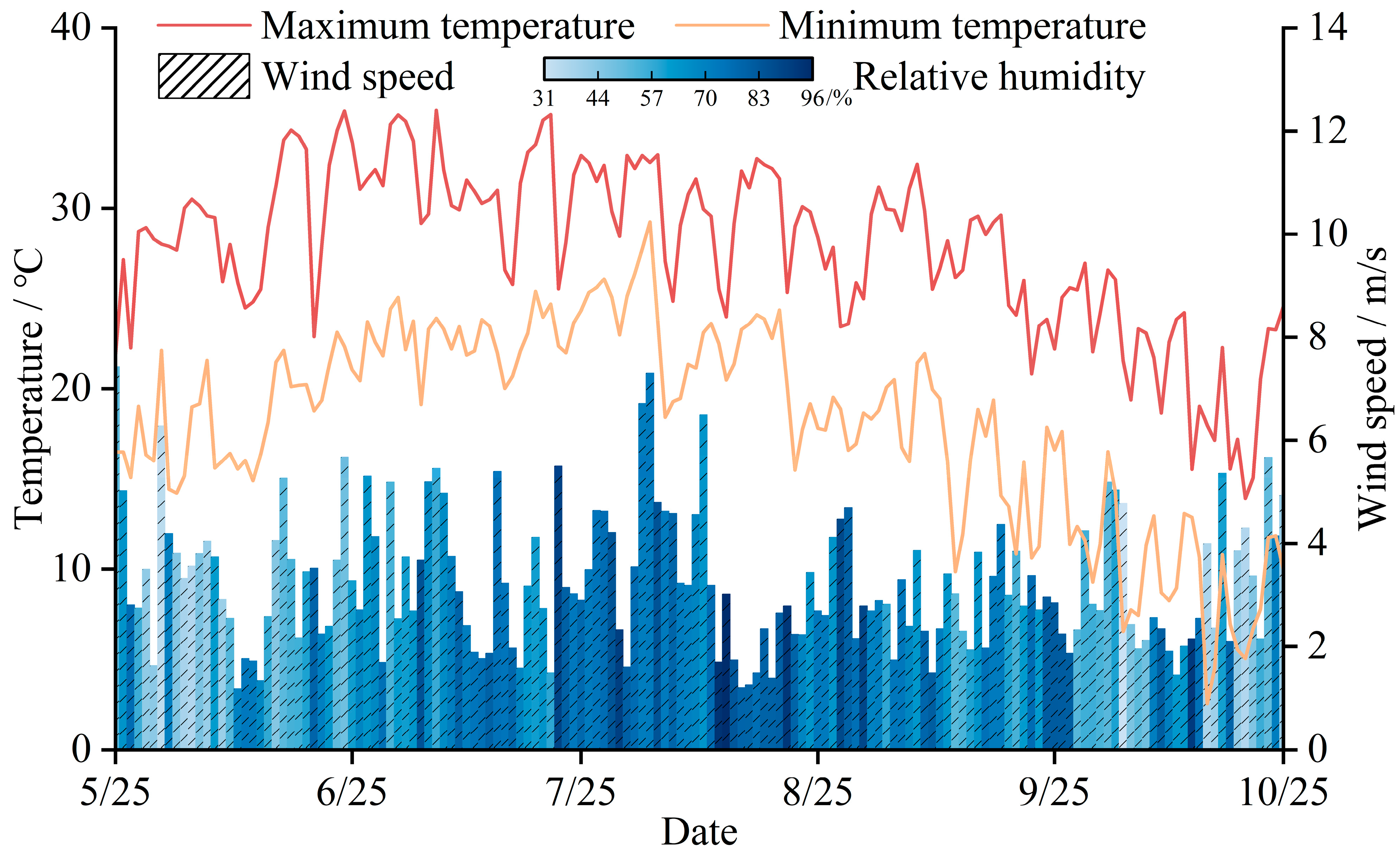
In this study, data of Days After Transplantation and Meteorological Factors (DATaMF) were collected. Among them, the number of days after transplanting is defined as the growth days of rice from the date of transplanting. It was primarily calculated manually based on the recorded transplanting date and the dates of experimental observations. Meteorological factors, including minimum temperature, maximum temperature, wind speed, and relative humidity, were obtained from the ERA5 hourly data on single levels from 1979 to present [19]. The daily data used in this study were derived from hourly data processed and organized by the WheatA system. The detailed statistical results of meteorological factors are shown in Figure 3.

2.3. Spectral Preprocessing

In the field of rice growth monitoring using UAV remote sensing, the accuracy of spectral data analysis is crucial. However, the collection of field spectral data is prone to interference from various environmental factors such as cloud cover, wind speed, and soil moisture content, resulting in a large amount of redundant noise information being mixed into the spectral curve and limiting the inversion accuracy of physical and chemical parameters of rice [20]. Therefore, in this study, Savitzky–Golay smoothing (R_SG) was applied to the UAV-collected spectral curves (R_UAV) using MATLAB R2024 [21].

In addition, the first derivative transformation represents the rate of change in the spectral curve and is one of the commonly used spectral transformation methods. It can enhance the spectral response characteristics to a certain extent [22,23,24], and its calculation formula is shown in Equation (1). Considering that the error in derivative calculation is directly related to the band interval $∆\lambda$, to ensure the calculation accuracy of derivative transformation, the spectral resolution of R_SG is resampled to a 1 nm interval (R_RS), and the first derivative transformation (R_FD) is performed on the spectral curve based on R_RS.

$${\mathrm{R}}_{\mathrm{FD}}\left({\lambda }_i\right)={\displaystyle \frac{d{\mathrm{R}}_{\mathrm{RS}}}{d\lambda }}\approx {\displaystyle \frac{{\mathrm{R}}_{\mathrm{RS}}\left({\lambda }_{i+1}\right)-{\mathrm{R}}_{\mathrm{RS}}\left({\lambda }_{i-1}\right)}{2∆\lambda }}$$

(1)

Among them, the ${\mathrm{R}}_{\mathrm{FD}}\left({\lambda }_i\right)$ represents the wavelength ${\lambda }_i$ reflectivity value after the first derivative transform, ${\mathrm{R}}_{\mathrm{RS}}\left({\lambda }_i\right)$ represents the wavelength ${\lambda }_i$ reflectivity, and $∆\lambda$ represents the adjacent wavelength interval.

2.4. Spectral Feature Extraction by Multi-Feature Band Selection Method

Considering that the spectral data obtained has a high dimension and strong correlation between bands, when dealing with the inversion problem in the small sample scenario, the computational complexity is relatively large, and it is prone to cause the “Hughes phenomenon” [25], which in turn affects the inversion accuracy of the physical and chemical parameters of rice. To improve computational efficiency and mitigate the interference of high-dimensional redundancy on feature selection, the spectral data of R_RS and R_FD are extracted at intervals of 5 nm before the selection of feature bands, reducing the spectral dimension.

In this study, three characteristic band selection methods, namely, SPA (Successive Projection Algorithm) [26], CARS (Competitive Adaptive Reweighted Sampling) [27] and Relief-F (Relevant Features) [28], were utilized—primarily implemented in MATLAB using the spa, carspls, and relief functions—to start from band independence, model contribution, and category separability, respectively, to achieve the characteristic band selection of multi-dimensional spectral data. SPA employs an iterative vector projection optimization approach to select band combinations with maximal information and minimal redundancy, making it suitable for handling strongly correlated spectral data [29]. CARS integrates an exponential decay function with adaptive reweighted sampling, emulating the “survival of the fittest” principle, which enhances model stability under small-sample conditions [30]. Relief-F is an instance-based filter feature selection method designed for multiclass problems [31]. It does not rely on a specific model and is relatively computationally efficient. Therefore, in this study, the above three methods were used to analyze the R_RS and R_FD at 5 nm intervals, and the characteristic band combinations that could effectively characterize the changes in rice LAI were screened out, providing key inputs for the subsequent construction of a small-sample hyperspectral inversion model of rice LAI.

2.5. Construction of Rice LAI Inversion Models Based on Different Machine Learning Algorithms

In order to systematically evaluate the impact of different machine learning algorithms on LAI inversion performance, this study selected three machine learning algorithms—Random Forests (RF) [32,33], Extreme Learning Machine (ELM) [34,35], and eXtreme Gradient Boosting (XGBoost) [36,37]—for constructing rice LAI inversion models. Prior to model construction, input data were normalized. Based on the experimental design, the input features were divided into two categories: one consisted of a subset of feature bands selected by feature selection methods from R_RS and R_FD; the other incorporated an extended feature set formed by adding DATaMF to the aforementioned inputs. By developing inversion models under these different feature combinations, this study aimed to capture the complex nonlinear relationships between spectra and rice LAI. Furthermore, to facilitate clearer comparison of inversion results across models, the R_RS, R_FD, R_RS-DATaMF, and R_FD-DATaMF datasets were split into training and testing sets in an 8:2 ratio, with consistent datasets ensured for the RF, ELM, and XGBoost models. The RF and ELM models were implemented in the MATLAB environment, primarily utilizing the built-in functions TreeBagger and elmtrain for model development, while XGBoost was implemented in Python 3.10.2 using the xgboost package 3.0.5.

2.6. Model Evaluation Method

In this study, the model performance was evaluated using the coefficient of determination (R²), Root Mean Square Error (RMSE), and Relative Prediction Deviation (RPD) as the evaluation indicators for the rice LAI inversion model [38,39], and the calculation formulas are shown in Equations (2)–(4). The size of R² is mainly used to evaluate the fitting effect of the inversion model. The closer it is to 1, the better the fitting effect. RMSE serves as an evaluation criterion for the degree of difference between the predicted values and the true values of the inversion model. The smaller the value, the higher the accuracy of the model. RPD assesses the stability of the inversion model by comparing the ratio of RMSE to the standard deviation of the true value. When RPD < 1.4, the reliability of the inversion model is insufficient. Conversely, the model has better stability.

$$R^2=1-{\displaystyle \frac{{\sum }_{j=1}^N{\left(y_{{real}_j}-{\widehat{y}}_{{pred}_j}\right)}^2}{{\sum }_{j=1}^N{\left(y_{{real}_j}-{\overline{y}}_{real}\right)}^2}}$$

(2)

$$\mathrm{RMSE}=\sqrt{{\displaystyle \frac{{\sum }_{j=1}^N{\left({\widehat{y}}_{{pred}_j}-y_{{real}_j}\right)}^2}{N}}}$$

(3)

$$\mathrm{RPD}={\displaystyle \frac{SD}{\mathrm{RMSE}}}$$

(4)

Among them, $y_{{real}_j}$ is the true value of the physicochemical parameter, ${\overline{y}}_{real}$ is the average value of the true value, ${\widehat{y}}_{{pred}_j}$ is the predicted value of the inversion model, $N$ is the total number of samples, and $SD$ is the standard deviation of the true value of the samples.

3. Results

3.1. Results of Spectral Pretreatment

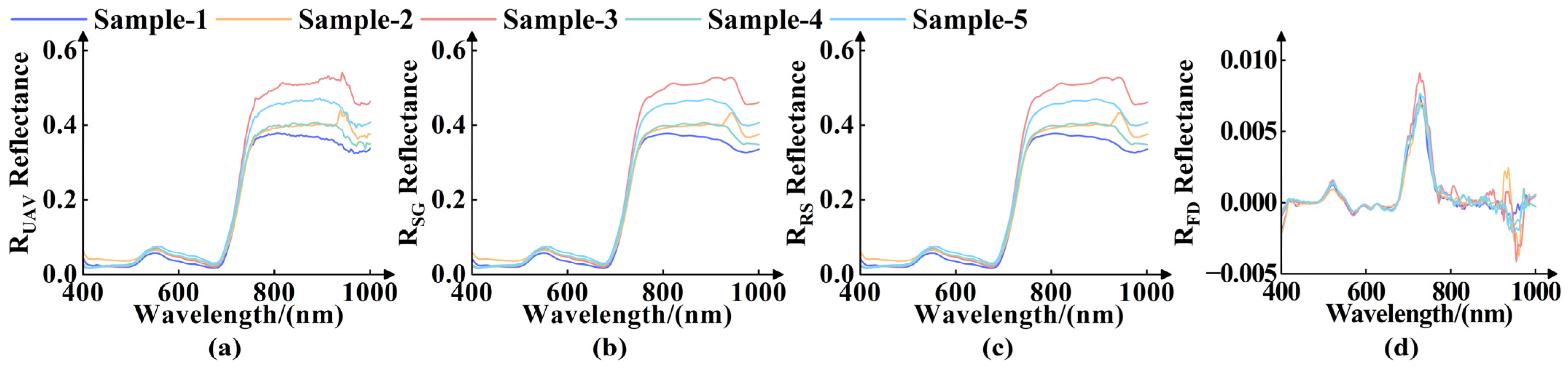
In this study, the acquired UAV spectral curves were preprocessed using the Savitzky–Golay smoothing, resampling, and first derivative transformation. The results are shown in Figure 4 (taking five samples as examples). Compared with Figure 4a, the Savitzky–Golay smoothing in Figure 4b significantly reduces the perturbation caused by moisture and environmental noise in the near-infrared region. It can be seen from Figure 4b,c that the spectral curve shape remains relatively stable after resampling. The result of the first derivative transformation is shown in Figure 4d. The spectral curve presents distinct peaks and troughs. That is, in the band region where the spectrum is relatively smooth and the rate of change is low in Figure 4c, the corresponding R_FD reflectance value approaches zero, forming a sharp and clear peak at the 720 nm band.

3.2. Spectral Feature Extraction Results Based on the Multi-Feature Band Selection Method

In this study, three feature selection methods, namely, SPA, CARS, and Relief-F, were used to extract the characteristic bands of LAI in the R_RS and R_FD spectra, respectively. The specific results are as follows:

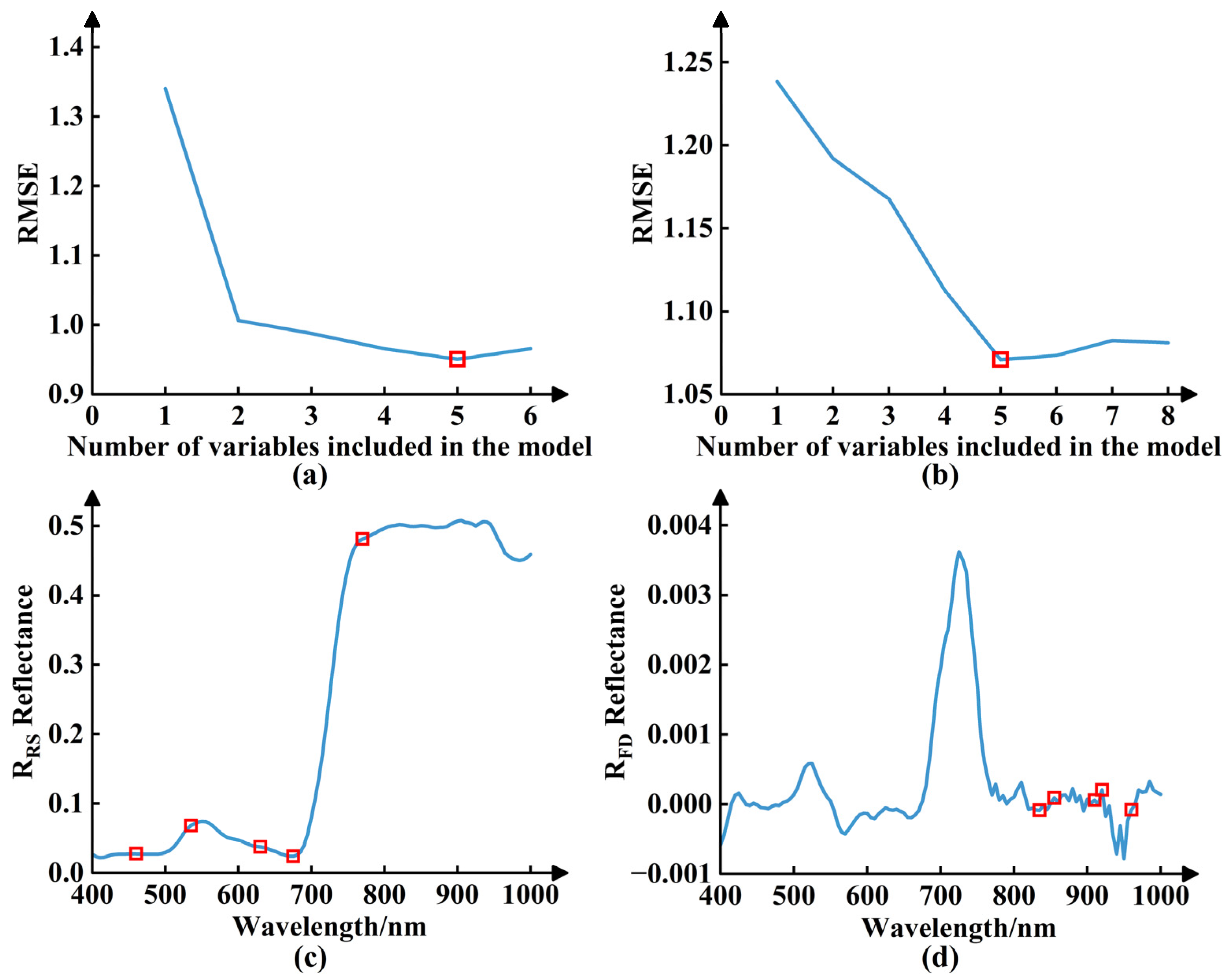
The feature bands selected by SPA are shown in Figure 5. It can be seen from Figure 5a,b that the overall trend of RMSE changes is roughly the same, first rapidly declining and then stabilizing. Moreover, the minimum RMSE is achieved when the number of variables is 5. The corresponding selected bands are indicated in Figure 5c,d. That is, five LAI characteristic bands were screened out from the R_RS and arranged in ascending order of the band sequence as 460, 535, 630, 675, and 770 nm, respectively. Five LAI characteristic bands were also screened out in the R_FD and arranged in ascending order of the band sequence as 835, 855, 910, 920, and 960 nm, respectively.

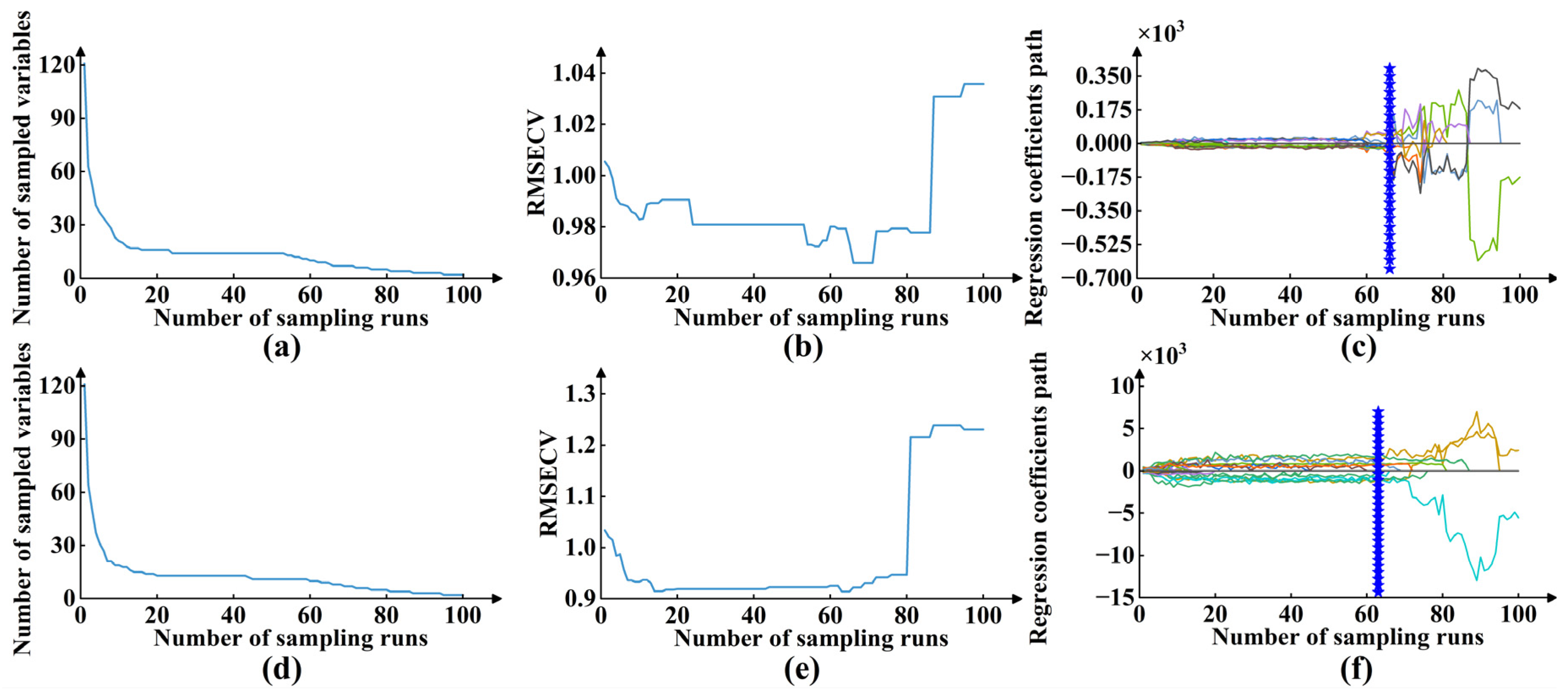
The feature bands selected by CARS are shown in Figure 6. It can be seen from the figure that as the number of iterations increases, the number of variables based on R_RS and R_FD feature selection represented in Figure 6a,d both decline rapidly and then stabilize. Their RMSECV values reach the minimum at the 66th and 63rd iterations, respectively, and the optimal iteration points are marked in Figure 6c,f. In this study, the CARS feature selection method was utilized to screen out seven LAI feature bands in R_RS. Arranged in ascending order of the band sequence, they were 685, 805, 810, 815, 820, 840, and 845 nm, respectively. Nine LAI characteristic bands were screened out from the R_FD and arranged in ascending order of the band sequence as 425, 665, 670, 755, 775, 810, 835, 910, and 985 nm.

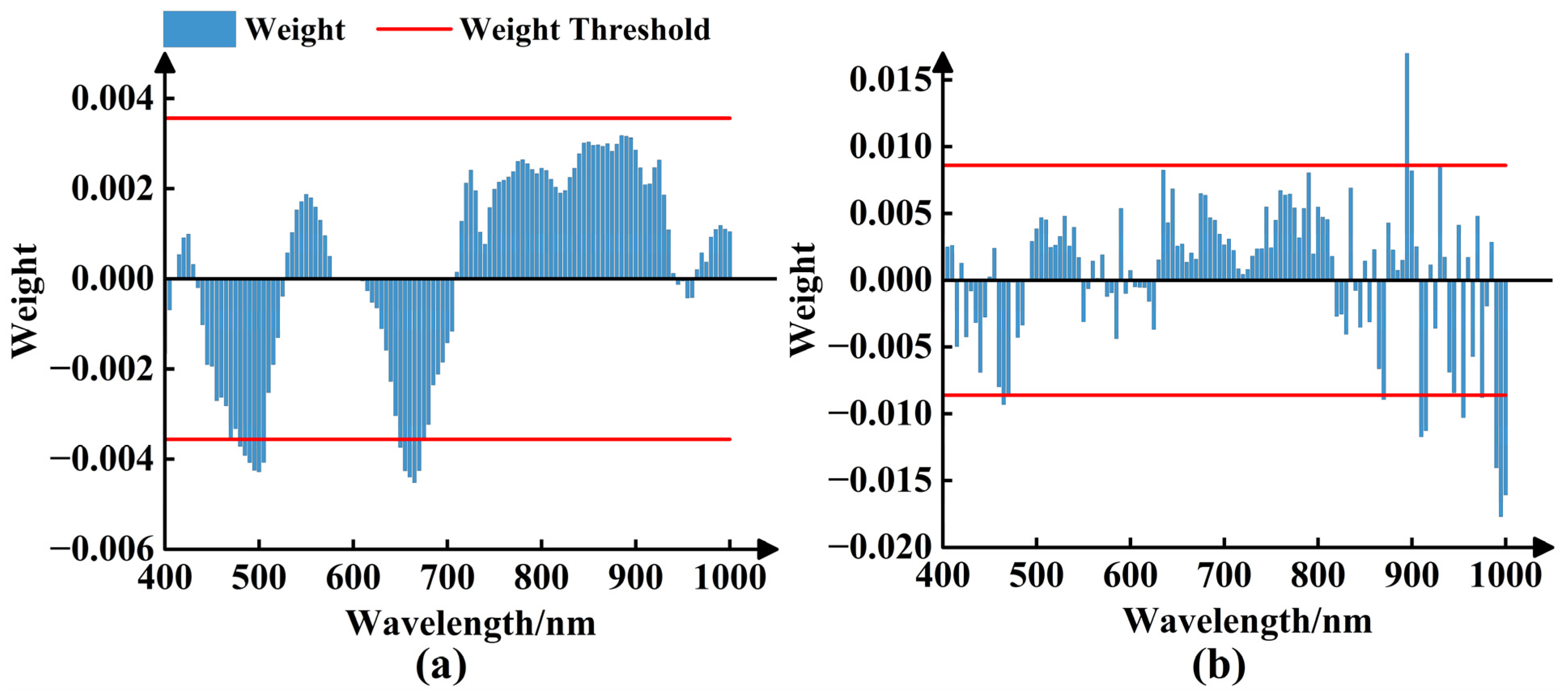
Relief-F assigns weights to features by comparing the categories of neighboring samples. The positive and negative values and their magnitudes, respectively, represent the correlation (positive and negative) between the spectral bands and LAI, as well as the strength of the correlation between the two. It then ranks them in importance and retains the top 10% of the characteristic bands with the highest weights. The band screening results are shown in Figure 7. The upper and lower red lines in the figure represent the weight thresholds, dividing the image into upper, middle, and lower parts. The positive and negative correlated feature bands selected are, respectively, located in the upper and lower parts of the figure. That is, in this study, twelve LAI characteristic bands were screened out in R_RS based on Relief-F, and they were arranged in ascending order of the band sequence as 480, 485, 490, 495, 500, 505, 650, 655, 660, 665, 670, and 675 nm. Twelve LAI characteristic bands were screened out from the R_FD and arranged in ascending order of the band sequence as 465, 470, 870, 895, 910, 915, 930, 955, 975, 990, 995, and 1000 nm.

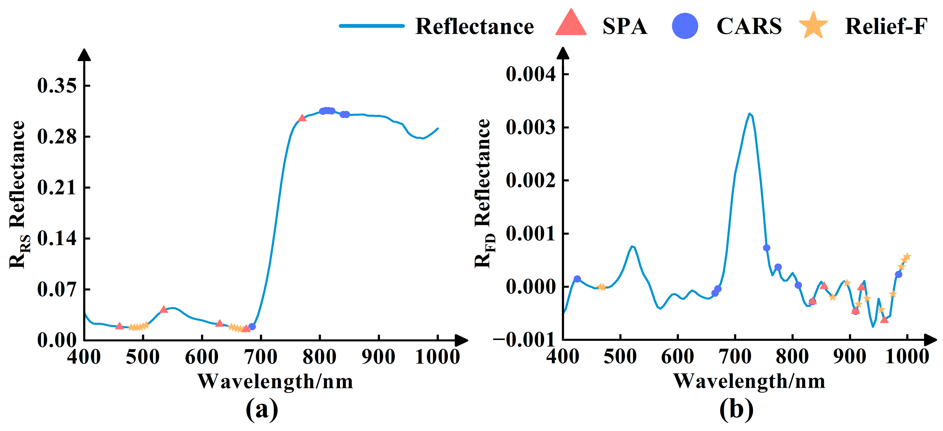
In summary, by comparing three different feature selection methods, namely, SPA, CARS, and Relief-F, this study found that they showed significant differences in R_RS and R_FD. The comparison results of the feature band screening are shown in Figure 8. In contrast, the SPA method can effectively capture the core spectral information of LAI inversion with very few bands. The screening results of the CARS method show obvious “cluster” characteristics, to a certain extent, retaining the synergy effect among continuous spectra. The screening results of the Relief-F method on R_RS are concentrated between 400 and 700 nm, while most of the screening results in R_FD are distributed between 800 and 1000 nm, indicating that the first derivative transformation can significantly enhance the spectral characteristics of the canopy structure in the near-infrared band.

3.3. Inversion Results of Rice LAI Models Based on Different Machine Learning Algorithms

3.3.1. Summary of Rice LAI Inversion Results Based on Different Machine Learning Algorithms

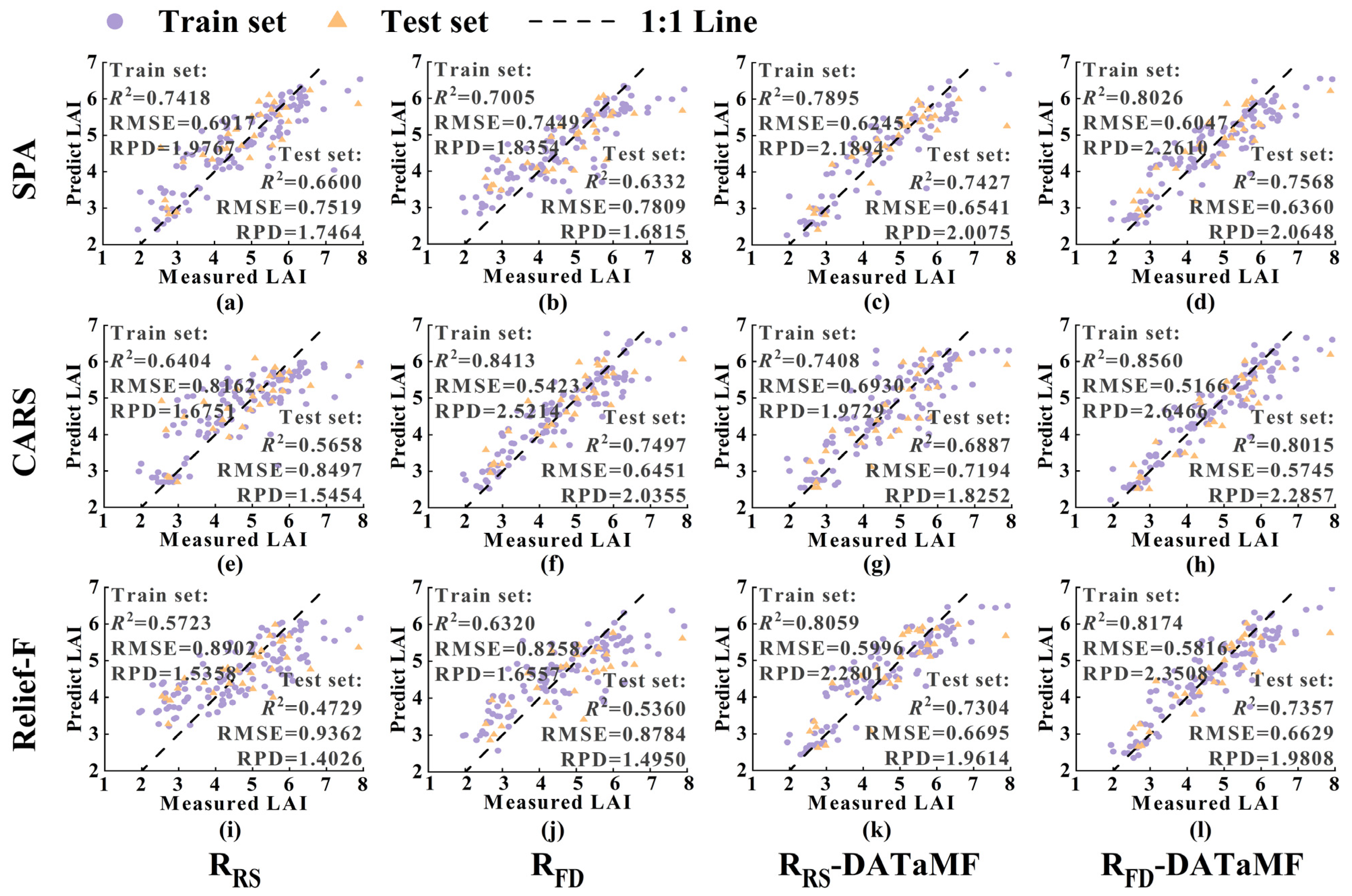
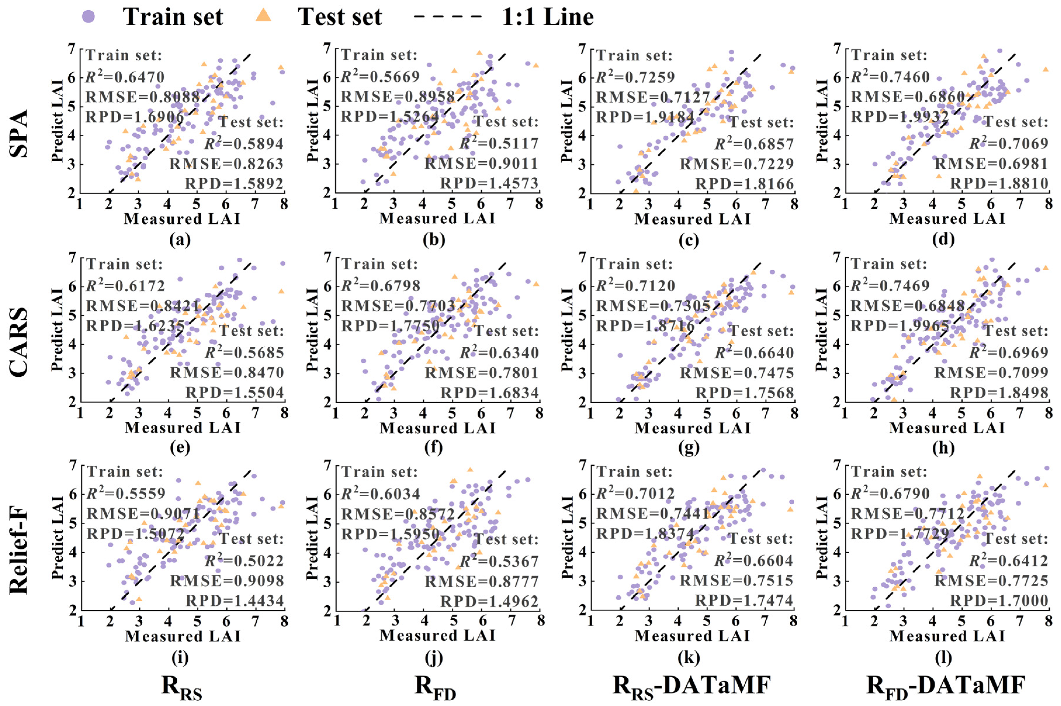
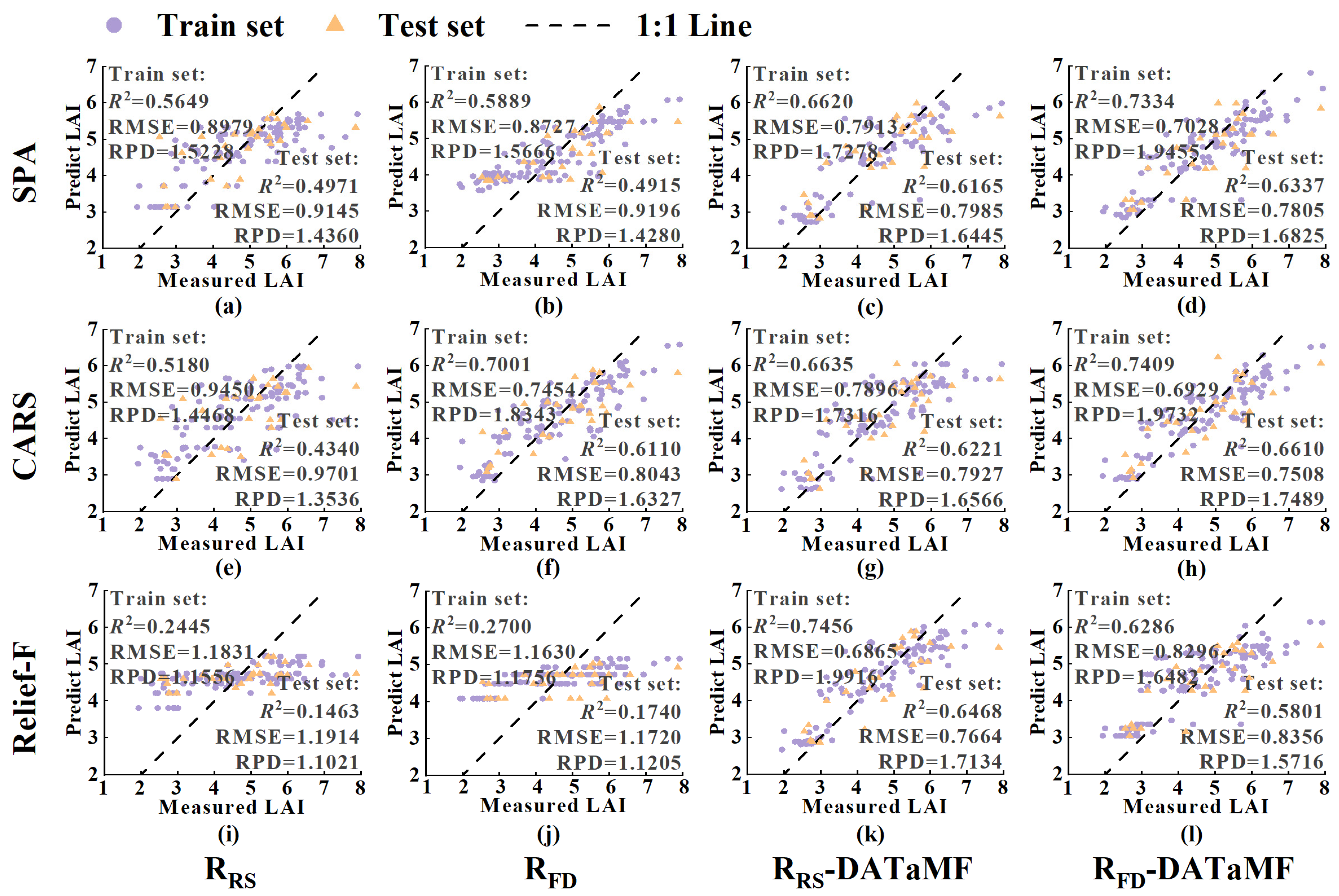
To systematically evaluate the impact of different input features and machine learning algorithms on the performance of rice LAI inversion, this study constructed LAI inversion models using RF, ELM, and XGBoost. The models were built using spectral data R_RS and R_FD processed by three feature selection methods (SPA, CARS, Relief-F), along with their fused versions with DATaMF (R_RS-DATaMF and R_FD-DATaMF). The inversion results of the top three optimal models under different machine learning algorithms are shown in

Table 1. Statistical performance comparison of the three best-performing rice LAI inversion models for different machine learning algorithms.

Machine Learning Algorithm	Input Features	Training Set			Test Set
		R2	RMSE	RPD	R2	RMSE	RPD
RF	CARS-RFD-DATaMF	0.8560	0.5166	2.6466	0.8015	0.5745	2.2857
	SPA-RFD-DATaMF	0.8026	0.6047	2.2610	0.7568	0.6360	2.0648
	CARS-RFD	0.8413	0.5423	2.5214	0.7497	0.6451	2.0355
ELM	SPA-RFD-DATaMF	0.7460	0.6860	1.9932	0.7069	0.6981	1.8810
	CARS-RFD-DATaMF	0.7469	0.6848	1.9965	0.6969	0.7099	1.8498
	SPA-RRS-DATaMF	0.7259	0.7127	1.9184	0.6857	0.7229	1.8166
XGBoost	CARS-RFD-DATaMF	0.7409	0.6929	1.9732	0.6610	0.7508	1.7489
	Relief-F-RRS-DATaMF	0.7456	0.6865	1.9916	0.6468	0.7664	1.7134
	SPA-RFD-DATaMF	0.7334	0.7028	1.9455	0.6337	0.7805	1.6825

, and the detailed fitting results of the models are shown in Figure 9, Figure 10 and Figure 11.

Overall, from the comprehensive inversion results in the figures, different spectral data preprocessing methods, feature selection algorithms, and the introduction of DATaMF significantly affected the performance of the LAI inversion models. Analyzing the nine inversion models in Table 1 from the perspective of feature selection methods reveals that only a few models were built based on feature bands selected by the Relief-F method. Furthermore, the inversion models built based on the CARS method generally outperformed those based on SPA. This indicates that the CARS method may have greater advantages in screening key features from the high-dimensional spectral data in this study.

A horizontal comparison of the three machine learning algorithms—RF, ELM, and XGBoost—showed that the inversion model built based on RF achieved the best fitting performance, with R², RMSE, and RPD values of 0.8015, 0.5745, and 2.2857, respectively, for the test set. In contrast, the best LAI inversion models under the ELM and XGBoost algorithms had test set R² values of 0.7069 and 0.6610, respectively, which were significantly lower than that of RF. This phenomenon preliminarily proves that when processing the fused data of spectrum and DATaMF, the RF algorithm may possess stronger anti-overfitting capabilities and a better ability to capture complex nonlinear relationships.

Additionally, another clear pattern emerged: among the top three inversion models for each of the RF, ELM, and XGBoost algorithms, the input features almost included the newly introduced DATaMF feature. This result indicates that introducing the DATaMF feature, which characterizes the rice growth process and meteorological data, has a significant positive incentive for improving the fitting performance of the LAI inversion model and substantially enhances the model’s explanatory power for the rice growth process.

3.3.2. Comprehensive Comparison of Inversion Performance of Rice LAI Models Based on Different Machine Learning Algorithms

To sum up, by comparing the results of Section 3.3.1 in this study, it can be known that the optimal LAI inversion model is RF-based CARS-R_FD-DATaMF, and the R², RMSE, and RPD of its training set are 0.8560, 0.5166, and 2.6466, respectively; the R², RMSE and RPD of the test set are 0.8015, 0.5745, and 2.2857, respectively. This study further provides a comprehensive analysis of the rice LAI inversion models from three perspectives: feature selection, machine learning algorithms, and the inclusion of DATaMF, as follows:

The average performance of models grouped by feature selection method is summarized in

Table 2. The training set results of LAI inversion models using different feature selection methods.

Performance Metrics	SPA		CARS		Relief-F
	With RRS	With RFD	With RRS	With RFD	With RRS	With RFD
R2	0.6885	0.6898	0.6487	0.7608	0.6042	0.6051
RMSE	0.7545	0.7511	0.8028	0.6587	0.8351	0.8380
RPD	1.8376	1.8547	1.7202	2.1245	1.7180	1.6997

and

Table 3. The test set results of LAI inversion models using different feature selection methods.

Performance Metrics	SPA		CARS		Relief-F
	With RRS	With RFD	With RRS	With RFD	With RRS	With RFD
R2	0.6319	0.6223	0.5905	0.6924	0.5265	0.5339
RMSE	0.7780	0.7860	0.8211	0.7380	0.8708	0.8665
RPD	1.7067	1.6992	1.6147	1.7901	1.5617	1.5607

. Among them, “With R_RS” represents the LAI inversion model constructed based on the two-input data of R_RS and R_RS-DATaMF. “With R_FD” represents the LAI inversion model constructed based on two types of input data: R_FD and R_FD-DatAMF. It can be seen that the characteristic bands based on the CARS method combined with R_FD screening exhibit the best fitting performance, and the inversion result of LAI is the best. Based on the above analysis, it can be known that the selection of feature selection methods needs to be combined with the actual requirements of the model and through specific research and analysis, which is consistent with the research conclusions of relevant scholars [40].

The average performance of models grouped by machine learning algorithms is summarized in

Table 4. The training set results of LAI inversion models using different machine learning algorithms.

Performance Metrics	RF		ELM		XGBoost
	With RRS	With RFD	With RRS	With RFD	With RRS	With RFD
R2	0.7151	0.7750	0.6598	0.6703	0.5664	0.6103
RMSE	0.7192	0.6360	0.7909	0.7775	0.8822	0.8344
RPD	1.9383	2.2118	1.7415	1.7765	1.5960	1.6906

and

Table 5. The test set results of LAI inversion models using different machine learning algorithms.

Performance Metrics	RF		ELM		XGBoost
	With RRS	With RFD	With RRS	With RFD	With RRS	With RFD
R2	0.6434	0.7021	0.6117	0.6212	0.4938	0.5252
RMSE	0.7635	0.6963	0.8008	0.7899	0.9056	0.8771
RPD	1.7481	1.9239	1.6506	1.6779	1.4844	1.5307

. From the results, whether “With R_RS” or “With R_FD”, RF achieved the best LAI inversion performance on both the training set and the test set. ELM’s performance is second, while XGBoost’s performance is relatively weak. This might be because RF can effectively reduce the model variance by constructing multiple decision trees and adopting the Bagging strategy. The random initialization weights of ELM may limit its full mining of complex nonlinear spectral features, while XGBoost, under a limited data scale, the mechanism of minimizing losses by constantly learning residuals is more susceptible to noise and outliers in the data. In conclusion, the rice LAI inversion model based on RF demonstrates superior robustness.

The average performance of models grouped by the inclusion of DATaMF is summarized in

Table 6. Results of the LAI inversion model training set before and after the introduction of DATaMF.

Performance Metrics	RF		ELM		XGBoost
	No DATaMF	DATaMF	No DATaMF	DATaMF	No DATaMF	DATaMF
R2	0.6880	0.8020	0.6117	0.7185	0.4811	0.6957
RMSE	0.7518	0.6033	0.8469	0.7216	0.9679	0.7488
RPD	1.8667	2.2835	1.6196	1.8983	1.4503	1.8363

and

Table 7. Results of the LAI inversion model test set before and after the introduction of DATaMF.

Performance Metrics	RF		ELM		XGBoost
	No DATaMF	DATaMF	No DATaMF	DATaMF	No DATaMF	DATaMF
R2	0.6029	0.7426	0.5571	0.6758	0.3923	0.6267
RMSE	0.8070	0.6527	0.8570	0.7337	0.9953	0.7874
RPD	1.6511	2.0209	1.5366	1.7919	1.3455	1.6696

. Among them, the LAI inversion models based on R_RS-DATaMF and R_FD-DATaMF are denoted as “DATaMF”, and the LAI inversion models based on R_RS and R_FD are denoted as “No DATaMF”. It can be seen that for the three machine learning algorithms of RF, ELM and XGBoost, the number of days after transplanting and meteorological factors, as the new feature sets introduced in this study, have both improved the robustness and accuracy of the rice LAI inversion model to a certain extent. Therefore, the introduction of DATaMF can provide new ideas for monitoring crop growth in dynamic environments.

4. Discussion

4.1. Analysis of the Results of Spectral Preprocessing and Characteristic Band Selection

This study implemented a three-stage preprocessing procedure comprising Savitzky–Golay smoothing (R_SG), resampling (R_RS), and first derivative transformation (R_FD). As can be seen from Figure 4a, R_UAV exhibits significant high-frequency fluctuations in the near-infrared region. This finding is consistent with the research results of Hong et al. [41], indicating that the process of collecting spectral data using UAVs is susceptible to unavoidable environmental factors such as leaf swaying caused by wind speed, cloud layer changes, and differences in soil background moisture [42]. The smoothed spectra R_SG effectively reduced noise while largely preserving the original spectral profile, thereby minimizing signal distortion and providing a more reliable basis for subsequent analysis. The effectiveness of this spectral smoothing method in the field of agricultural remote sensing has been widely verified by numerous scholars [43,44]. The calculation accuracy of the first derivative transformation depends on the uniformity and precision of the wavelength segment interval ($∆\lambda$) [45], which has been confirmed by scholars to be an effective spectral processing method [46]. Resampling the smoothed R_SG to a high-resolution interval of 1 nm can fundamentally reduce the computational error introduced by the band interval problem and further magnify the spectral details related to the physical and chemical parameters of rice.

As can be seen from the comparison of multi-feature selection results in Figure 8, there are significant differences in location and quantity among the three feature selection methods, namely SPA (Successive Projection Algorithm), CARS (Competitive Adaptive Reweighted Sampling), and Relief-F (Relevant Features). For example, SPA only selects spectral bands with low collinearity, resulting in relatively discrete selected bands, which is consistent with the findings of Li et al. [47]. Judging from the distribution of characteristic bands selected by CARS in R_RS and R_FD, the spectral features are distributed in different regions, corroborating the results of Wang et al. [48] that CARS can screen the band combinations with the greatest contribution to the model across the full band range. In contrast, the Relief-F method obtains spectral features containing more bands, and its selection results in R_RS and R_FD are concentrated in the visible light region and near-infrared region, respectively, showing a certain clustering phenomenon, which aligns with the conclusions of Ren et al. [49] regarding dimensionality reduction in hyperspectral images. From the results in Table 2 and Table 3, it can be seen that the reason why the inversion model constructed by CARS combined with R_FD can achieve the best fitting effect may be that R_FD amplifies the features of the near-infrared region, and the adaptive re-weighted sampling mechanism of CARS can effectively deal with the overfitting problem under small sample data. The results of this study are consistent with the findings of Liu et al. [50], that is, the feature selection strategy combined with derivative transformation performs better than the inversion using R_RS.

4.2. The Influence of Different Machine Learning Algorithms and the Introduction of DATaMF on the Performance of Rice LAI Inversion Models

This study systematically evaluated the LAI inversion performance of three machine learning algorithms, namely, Random Forests (RF), Extreme Learning Machine (ELM), and eXtreme Gradient Boosting (XGBoost), before and after the introduction of the Days After Transplantation and Meteorological Factors (DATaMF) after rice transplantation. The results in Table 4 and Table 5 show that, under the same input data, there are significant differences in the LAI fitting effects based on different machine learning algorithms. This phenomenon is similar to that observed by Zhang et al. [51] in estimating grassland aboveground biomass based on multiple machine learning algorithms. Among the inversion results of this study, RF demonstrated superior inversion performance. This might be because RF improves its generalization performance for small-sample data and high-dimensional features and is less affected by the noise and multicollinearity present in spectral data. This is consistent with the findings of Zhou et al. [52], that is, no inversion method is always optimal, but RF usually demonstrates a strong fitting ability.

One of the core innovations of this study is to input DATaMF as an additional new feature set along with the spectrum into the inversion model. The results in Table 6 and Table 7 indicate that the introduction of DATaMF can enhance the accuracy and robustness of the model regardless of the machine learning algorithm used. It is worth affirming that this conclusion is consistent with that of Zare et al. [53], who introduced weather data for crop yield prediction. This is mainly because LAI increases significantly from the tillering stage to the heading stage [54], and the number of days after transplanting is an effective data that can characterize the physiological stage differences in rice. This highly resembles the view of Graf et al. [55] that phenological information is an important support for agricultural decision-making. Secondly, meteorological conditions of high temperature and low humidity are prone to cause rice to curl. Strong wind conditions will increase the disturbance of the canopy structure, leading to spectral noise and subsequently affecting the canopy spectrum. In the study of Fan et al. [56] on estimating potato yield, the importance of environmental variables was also recognized, and these data were successfully used to achieve the most accurate potato yield estimation [57].

However, this study also has some limitations. The limited diversity of meteorological factors and rice varieties may limit the generalizability of the model. Secondly, the quantification of the contributions from meteorological factors and their interactions requires further in-depth analysis. Future research could be extended to multiple regions and varieties to further validate the model’s transferability.

5. Conclusions

In this study, to improve the accuracy of UAV hyperspectral inversion of rice LAI under the condition of small samples, we proposed an inversion method integrating Days After Transplanting and Meteorological Factors (DATaMF) data. By systematically comparing different spectral preprocessing schemes, feature selection algorithms, and machine learning models, the following main conclusions are drawn:

(1)

The three-level preprocessing procedure—comprising the Savitzky–Golay smoothing (R_SG), resampling (R_RS), and first derivative transformation (R_FD)—effectively eliminates environmental noise and enhances spectral features, thereby providing high-quality input for subsequent modeling. The spectral subset selected by Competitive Adaptive Reweighted Sampling (CARS) in combination with R_FD further improves the model’s performance in estimating rice LAI.

(2)

The introduction of the DATaMF feature set significantly enhances the accuracy and robustness of the LAI inversion model. Results indicate that after integrating DATaMF, the test set exhibits an average increase in R² of approximately 0.1643, an average decrease in RMSE of approximately 0.1618, and an average increase in RPD of 0.3164.

(3)

Among the three machine learning algorithms—RF, ELM, and XGBoost—the RF-based CARS-R_FD-DATaMF model achieves the best inversion performance, with test set R², RMSE, and RPD values of 0.8015, 0.5745, and 2.2857, respectively. This model is capable of meeting the requirements for precise and dynamic monitoring of LAI throughout the rice growth process.

References

1. Liu, Y.; Wang, B.; Tao, J.F.; Tian, S.J.; Sheng, Q.H.; Li, J.; Wang, S.W.; Liu, X.L.; He, H.L. Canopy structure dynamics constraints and time sequence alignment for improving retrieval of rice leaf area index from multi-temporal Sentinel-1 imagery. Comput. Electron. Agric. 2024, 227, 109658. [Google Scholar] [CrossRef] [Scilit]
2. Jin, Z.Y.; Liu, H.Z.; Cao, H.N.; Li, S.L.; Yu, F.H.; Xu, T.Y. Hyperspectral Remote Sensing Estimation of Rice Canopy LAI and LCC by UAV Coupled RTM and Machine Learning. Agriculture 2025, 15, 11. [Google Scholar] [CrossRef] [Scilit]
3. Yuan, W.S.; Meng, Y.; Li, Y.; Ji, Z.G.; Kong, Q.M.; Gao, R.; Su, Z.B. Research on rice leaf area index estimation based on fusion of texture and spectral information. Comput. Electron. Agric. 2023, 211, 108016. [Google Scholar] [CrossRef] [Scilit]
4. Wei, H.H.; Geng, X.Y.; Zhang, X.; Zhu, W.; Zhang, X.B.; Chen, Y.L.; Huo, Z.Y.; Zhou, G.S.; Meng, T.Y.; Dai, Q.G. Grain Yield, Biomass Accumulation, and Leaf Photosynthetic Characteristics of Rice under Combined Salinity-Drought Stress. Rice Sci. 2024, 31, 118–128. [Google Scholar] [CrossRef] [Scilit]
5. Wu, T.Z.; Zhang, Z.W.; Wang, Q.; Jin, W.J.; Meng, K.; Wang, C.; Yin, G.F.; Xu, B.D.; Shi, Z.H. Estimating rice leaf area index at multiple growth stages with Sentinel-2 data: An evaluation of different retrieval algorithms. Eur. J. Agron. 2024, 161, 127362. [Google Scholar] [CrossRef] [Scilit]
6. Du, R.Q.; Chen, J.Y.; Xiang, Y.Z.; Zhang, Z.T.; Yang, N.; Yang, X.Z.; Tang, Z.J.; Wang, H.; Wang, X.; Shi, H.Z.; et al. Incremental learning for crop growth parameters estimation and nitrogen diagnosis from hyperspectral data. Comput. Electron. Agric. 2023, 215, 108356. [Google Scholar] [CrossRef] [Scilit]
7. Yu, F.H.; Bai, J.C.; Jin, Z.Y.; Guo, Z.H.; Yang, J.X.; Chen, C.L. Combining the critical nitrogen concentration and machine learning algorithms to estimate nitrogen deficiency in rice from UAV hyperspectral data. J. Integr. Agric. 2023, 22, 1216–1229. [Google Scholar] [CrossRef] [Scilit]
8. Guo, A.T.; Ye, H.C.; Huang, W.J.; Qian, B.X.; Wang, J.J.; Lan, Y.B.; Wang, S.Z. Inversion of maize leaf area index from UAV hyperspectral and multispectral imagery. Comput. Electron. Agric. 2023, 212, 108020. [Google Scholar] [CrossRef] [Scilit]
9. Zhou, Y.X.; Li, X.J.; Chen, C.; Zhou, L.; Zhao, Y.Y.; Chen, J.J.; Tan, C.; Sun, J.Q.; Zhang, L.J.; Hu, M.C.; et al. Coupling the PROSAIL Model and Machine Learning Approach for Canopy Parameter Estimation of Moso Bamboo Forests from UAV Hyperspectral Data. Forests 2024, 15, 946. [Google Scholar] [CrossRef] [Scilit]
10. Li, J.T.; Wijewardane, N.K.; Ge, Y.F.; Shi, Y.Y. Improved chlorophyll and water content estimations at leaf level with a hybrid radiative transfer and machine learning model. Comput. Electron. Agric. 2023, 206, 107669. [Google Scholar] [CrossRef] [Scilit]
11. Kamal, M.; Phinn, S.; Johansen, K. Assessment of multi-resolution image data for mangrove leaf area index mapping. Remote Sens. Environ. 2016, 176, 242–254. [Google Scholar] [CrossRef] [Scilit]
12. Garofalo, S.P.; Ardito, F.; Sanitate, N.; De Carolis, G.; Ruggieri, S.; Giannico, V.; Rana, G.; Ferrara, R.M. Robustness of Actual Evapotranspiration Predicted by Random Forest Model Integrating Remote Sensing and Meteorological Information: Case of Watermelon (Citrullus lanatus, (Thunb.) Matsum. & Nakai, 1916). Water 2025, 17, 323. [Google Scholar] [CrossRef] [Scilit]
13. Duan, B.; Liu, Y.; Gong, Y.; Peng, Y.; Wu, X.; Zhu, R.; Fang, S. Remote estimation of rice LAI based on Fourier spectrum texture from UAV image. Plant Methods 2019, 15, 124. [Google Scholar] [CrossRef] [Scilit] [PubMed]
14. Liang, L.; Huang, T.; Di, L.P.; Geng, D.; Yan, J.; Wang, S.G.; Wang, L.J.; Li, L.; Chen, B.Q.; Kang, J.R. Influence of Different Bandwidths on LAI Estimation Using Vegetation Indices. IEEE J. Sel. Top. Appl. Earth Obs. Remote Sens. 2020, 13, 1494–1502. [Google Scholar] [CrossRef] [Scilit]
15. Kganyago, M.; Adjorlolo, C.; Mhangara, P.; Tsoeleng, L. Optical remote sensing of crop biophysical and biochemical parameters: An overview of advances in sensor technologies and machine learning algorithms for precision agriculture. Comput. Electron. Agric. 2024, 218, 108730. [Google Scholar] [CrossRef] [Scilit]
16. Qi, H.M.; Chen, A.; Yang, X.C.; Xing, X.Y. Estimation of crude protein content in natural pasture grass using unmanned aerial vehicle hyperspectral data. Comput. Electron. Agric. 2025, 229, 109714. [Google Scholar] [CrossRef] [Scilit]
17. Liu, K.; Zhou, Q.B.; Wu, W.B.; Xia, T.; Tang, H.J. Estimating the crop leaf area index using hyperspectral remote sensing. J. Integr. Agric. 2016, 15, 475–491. [Google Scholar] [CrossRef] [Scilit]
18. Li, S.L.; Jin, Z.Y.; Bai, J.C.; Xiang, S.; Xu, C.Y.; Yu, F.H. Research on fertilization decision method for rice tillering stage based on the coupling of UAV hyperspectral remote sensing and WOFOST. Front. Plant Sci. 2024, 15, 1405239. [Google Scholar] [CrossRef] [Scilit]
19. Hersbach, H.; Bell, B.; Berrisford, P.; Biavati, G.; Horányi, A.; Muñoz Sabater, J.; Nicolas, J.; Peubey, C.; Radu, R.; Rozum, I.; et al. ERA5 hourly data on single levels from 1940 to present. Copernic. Clim. Change Serv. C3S Clim. Data Store CDS 2023. [Google Scholar] [CrossRef]
20. Gao, C.R.; Li, H.; Wang, J.C.; Zhang, X.; Huang, K.M.; Song, X.Y.; Yang, W.D.; Feng, M.C.; Xiao, L.J.; Zhao, Y.; et al. Combined use of spectral resampling and machine learning algorithms to estimate soybean leaf chlorophyll. Comput. Electron. Agric. 2024, 218, 108675. [Google Scholar] [CrossRef] [Scilit]
21. Lu, B.; Liu, N.; Li, H.; Yang, K.; Hu, C.; Wang, X.; Li, Z.; Shen, Z.; Tang, X. Quantitative determination and characteristic wavelength selection of available nitrogen in coco-peat by NIR spectroscopy. Soil Tillage Res. 2019, 191, 266–274. [Google Scholar] [CrossRef] [Scilit]
22. Song, G.M.; Wang, Q.; Jin, J. Estimation of leaf photosynthetic capacity parameters using spectral indices developed from fractional-order derivatives. Comput. Electron. Agric. 2023, 212, 108068. [Google Scholar] [CrossRef] [Scilit]
23. Jin, J.; Wang, Q. Hyperspectral indices developed from the low order fractional derivative spectra can capture leaf dry matter content across a variety of species better. Agric. For. Meteorol. 2022, 322, 109007. [Google Scholar] [CrossRef] [Scilit]
24. Xiao, B.; Li, S.Z.; Dou, S.Q.; He, H.C.; Fu, B.L.; Zhang, T.X.; Sun, W.W.; Yang, Y.L.; Xiong, Y.K.; Shi, J.K.; et al. Comparison of leaf chlorophyll content retrieval performance of citrus using FOD and CWT methods with field-based full-spectrum hyperspectral reflectance data. Comput. Electron. Agric. 2024, 217, 108559. [Google Scholar] [CrossRef] [Scilit]
25. Hughes, G. On the mean accuracy of statistical pattern recognizers. IEEE Trans. Inf. Theory 1968, 14, 55–63. [Google Scholar] [CrossRef] [Scilit]
26. Zhang, B.Y.; Gu, L.M.; Dai, M.L.; Bao, X.Y.; Sun, Q.; Zhang, M.Z.; Qu, X.Z.; Li, Z.H.; Zhen, W.C.; Gu, X.H. Estimation of grain filling rate of winter wheat using leaf chlorophyll and LAI extracted from UAV images. Field Crops Res. 2024, 306, 109198. [Google Scholar] [CrossRef] [Scilit]
27. Zhou, X.F.; Sun, R.J.; Zhang, Z.J.; Song, Y.Y.; Jin, L.J.; Yuan, L. Improved Leaf Chlorophyll Content Estimation with Deep Learning and Feature Optimization Using Hyperspectral Measurements. Phyton-Int. J. Exp. Bot. 2025, 94, 503–519. [Google Scholar] [CrossRef] [Scilit]
28. Zhang, H.Y.; He, L.; Chen, Q.W.; Abdulraheem, M.I.; Ma, G.; Zhang, Y.F.; Gu, J.J.; Hu, J.D.; Wang, C.Y.; Feng, W. Multi-angular spectroscopic detection of winter wheat nitrogen fertilizer utilization status using integrated feature selection and machine learning. Comput. Electron. Agric. 2025, 231, 109916. [Google Scholar] [CrossRef] [Scilit]
29. Yan, K.T.; Song, X.B.; Yang, J.; Xiao, J.Q.; Xu, X.D.; Guo, J.; Zhu, H.Y.; Lan, Y.B.; Zhang, Y.L. Citrus huanglongbing detection: A hyperspectral data-driven model integrating feature band selection with machine learning algorithms. Crop Prot. 2025, 188, 107008. [Google Scholar] [CrossRef] [Scilit]
30. Wang, Z.L.; Huang, W.Q.; Li, J.B.; Liu, S.Q.; Fan, S.X. Assessment of protein content and insect infestation of maize seeds based on on-line near-infrared spectroscopy and machine learning. Comput. Electron. Agric. 2023, 211, 107969. [Google Scholar] [CrossRef] [Scilit]
31. Spolaôr, N.; Cherman, E.A.; Monard, M.C.; Lee, H.D. ReliefF for Multi-label Feature Selection. In Proceedings of the 2nd Brazilian Conference on Intelligent Systems (BRACIS), Fortaleza, Brazil, 19–24 October 2013; pp. 6–11. [Google Scholar]
32. Ihalainen, O.; Sandmann, T.; Rascher, U.; Mottus, M. Illumination correction for close-range hyperspectral images using spectral invariants and random forest regression. Remote Sens. Environ. 2024, 315, 114467. [Google Scholar] [CrossRef] [Scilit]
33. Guo, S.; Feng, Z.; Wang, P.; Chang, J.; Han, H.; Li, H.; Chen, C.; Du, W. Mapping and Classification of the Liaohe Estuary Wetland Based on the Combination of Object-Oriented and Temporal Features. IEEE Access 2024, 12, 60496–60512. [Google Scholar] [CrossRef] [Scilit]
34. Huang, G.B.; Zhu, Q.Y.; Siew, C.K. Extreme learning machine: Theory and applications. Neurocomputing 2006, 70, 489–501. [Google Scholar] [CrossRef] [Scilit]
35. Li, S.; Jin, Z.; Wang, N.; Guo, S.; Bai, J.; Yu, F.; Tian, M. Research on the optimal fertilization decision method for rice economy based on PROSAIL-WOFOST optimal coupling unit. Comput. Electron. Agric. 2025, 238, 110840. [Google Scholar] [CrossRef] [Scilit]
36. Ye, M.; Zhu, L.; Li, X.; Ke, Y.; Huang, Y.; Chen, B.; Yu, H.; Li, H.; Feng, H. Estimation of the soil arsenic concentration using a geographically weighted XGBoost model based on hyperspectral data. Sci. Total Environ. 2023, 858, 159798. [Google Scholar] [CrossRef] [Scilit]
37. Guan, Q.; Qiao, S.; Feng, S.; Du, W. Investigation of Peanut Leaf Spot Detection Using Superpixel Unmixing Technology for Hyperspectral UAV Images. Agriculture 2025, 15, 597. [Google Scholar] [CrossRef] [Scilit]
38. Xu, L.C.; Su, X.Y.; Wang, K.T.; Zhou, T.; Lu, C.H.; Niu, J.Q.; Jin, X.C.; Huang, J.Q.; Feng, H.L. Enhancing canopy nitrogen estimation in Torreya Grandis based on advanced SLIC-EVI and HMT-seCNN methods using hyperspectral UAV data. Comput. Electron. Agric. 2025, 231, 109977. [Google Scholar] [CrossRef] [Scilit]
39. Xiang, S.; Bai, J.C.; Jin, Z.Y.; Li, S.L.; Yu, F.H.; Xu, T.Y. PIOSL-5 With Nitrogen as an Independent Input Parameter and Accurate Estimation of Leaf Nitrogen. IEEE Trans. Geosci. Remote Sens. 2025, 63, 5513813. [Google Scholar] [CrossRef] [Scilit]
40. Bai, J.; Zhu, S.Y.; Hao, Y.C.; Li, X.Z.; Yang, C.B.; Wang, C.; Qiao, X.X.; Feng, M.C.; Xiao, L.J.; Song, X.Y.; et al. Comparative analysis of the effects of different dimensionality reduction algorithms on hyperspectral estimation of total nitrogen content in wheat soils. Eur. J. Agron. 2025, 168, 127660. [Google Scholar] [CrossRef] [Scilit]
41. Hong, Y.; Guo, L.; Chen, S.; Linderman, M.; Mouazen, A.M.; Yu, L.; Chen, Y.; Liu, Y.; Liu, Y.; Cheng, H.; et al. Exploring the potential of airborne hyperspectral image for estimating topsoil organic carbon: Effects of fractional-order derivative and optimal band combination algorithm. Geoderma 2020, 365, 114228. [Google Scholar] [CrossRef] [Scilit]
42. Gao, J.; Meng, B.; Liang, T.; Feng, Q.; Ge, J.; Yin, J.; Wu, C.; Cui, X.; Hou, M.; Liu, J.; et al. Modeling alpine grassland forage phosphorus based on hyperspectral remote sensing and a multi-factor machine learning algorithm in the east of Tibetan Plateau, China. ISPRS J. Photogramm. Remote Sens. 2019, 147, 104–117. [Google Scholar] [CrossRef] [Scilit]
43. Tan, J.; Ding, J.; Wang, Z.; Han, L.; Wang, X.; Li, Y.; Zhang, Z.; Meng, S.; Cai, W.; Hong, Y. Estimating soil salinity in mulched cotton fields using UAV-based hyperspectral remote sensing and a Seagull Optimization Algorithm-Enhanced Random Forest Model. Comput. Electron. Agric. 2024, 221, 109017. [Google Scholar] [CrossRef] [Scilit]
44. Yang, Z.; Tian, J.; Wang, Z.; Feng, K. Monitoring the photosynthetic performance of grape leaves using a hyperspectral-based machine learning model. Eur. J. Agron. 2022, 140, 126589. [Google Scholar] [CrossRef] [Scilit]
45. Tsai, F.; Philpot, W. Derivative Analysis of Hyperspectral Data. Remote Sens. Environ. 1998, 66, 41–51. [Google Scholar] [CrossRef] [Scilit]
46. Yu, Y.; Yu, H.; Li, X.; Zhang, L.; Sui, Y. Prediction of Potassium Content in Rice Leaves Based on Spectral Features and Random Forests. Agronomy 2023, 13, 2337. [Google Scholar] [CrossRef] [Scilit]
47. Song, L.; Wang, L.; Yang, Z.; He, L.; Feng, Z.; Duan, J.; Feng, W.; Guo, T. Comparison of algorithms for monitoring wheat powdery mildew using multi-angular remote sensing data. Crop J. 2022, 10, 1312–1322. [Google Scholar] [CrossRef] [Scilit]
48. Wang, Y.; Chen, S.; Hong, Y.; Hu, B.; Peng, J.; Shi, Z. A comparison of multiple deep learning methods for predicting soil organic carbon in Southern Xinjiang, China. Comput. Electron. Agric. 2023, 212, 108067. [Google Scholar] [CrossRef] [Scilit]
49. Ren, J.; Wang, R.; Liu, G.; Feng, R.; Wang, Y.; Wu, W. Partitioned Relief-F Method for Dimensionality Reduction of Hyperspectral Images. Remote Sens. 2020, 12, 1104. [Google Scholar] [CrossRef] [Scilit]
50. Liu, H.; Chen, J.Y.; Xiang, Y.Z.; Geng, H.S.; Yang, X.Z.; Yang, N.; Du, R.Q.; Wang, Y.; Zhang, Z.T.; Shi, L.S.; et al. Improving UAV hyperspectral monitoring accuracy of summer maize soil moisture content with an ensemble learning model fusing crop physiological spectral responses. Eur. J. Agron. 2024, 160, 127299. [Google Scholar] [CrossRef] [Scilit]
51. Zhang, R.; Feng, Q.; Zhang, Y.; Mai, J.; Liang, T. Estimation and trend analysis of grassland aboveground biomass on the Qinghai-Xizang Plateau based on machine learning. Ecol. Indic. 2025, 177, 113715. [Google Scholar] [CrossRef] [Scilit]
52. Zhou, X.J.; Liang, B.; He, J.N.; He, W. Accurate leaf area index estimation for Eucalyptus grandis using machine learning method with GF-6 WFV-A case study for Huangmian town, China. Front. For. Glob. Change 2024, 7, 1420533. [Google Scholar] [CrossRef] [Scilit]
53. Zare, H.; Viswanathan, M.; Weber, T.K.D.; Ingwersen, J.; Nowak, W.; Gayler, S.; Streck, T. Improving winter wheat yield prediction by accounting for weather and model parameter uncertainty while assimilating LAI and updating weather data within a crop model. Eur. J. Agron. 2024, 156, 127149. [Google Scholar] [CrossRef] [Scilit]
54. Fukuda, S.; Koba, K.; Okamura, M.; Watanabe, Y.; Hosoi, J.; Nakagomi, K.; Maeda, H.; Kondo, M.; Sugiura, D. Novel technique for non-destructive LAI estimation by continuous measurement of NIR and PAR in rice canopy. Field Crops Res. 2021, 263, 108070. [Google Scholar] [CrossRef] [Scilit]
55. Graf, L.V.; Merz, Q.N.; Walter, A.; Aasen, H. Insights from field phenotyping improve satellite remote sensing based in-season estimation of winter wheat growth and phenology. Remote Sens. Environ. 2023, 299, 113860. [Google Scholar] [CrossRef] [Scilit]
56. Fan, Y.; Liu, Y.; Yue, J.; Jin, X.; Chen, R.; Bian, M.; Ma, Y.; Yang, G.; Feng, H. Estimation of potato yield using a semi-mechanistic model developed by proximal remote sensing and environmental variables. Comput. Electron. Agric. 2024, 223, 109117. [Google Scholar] [CrossRef] [Scilit]
57. Yang, J.; Zhang, Y.-Z.; He, H.-H.; Li, Y.-C.; Chen, X.-R.; Bian, J.-M.; Jin, G.-H.; Li, X.-X.; Huang, S.-E. Current status and research advances of high-temperature hazards in rice. Ying Yong Sheng Tai Xue Bao J. Appl. Ecol. 2020, 31, 2817–2830. [Google Scholar] [CrossRef] [Scilit]
Figure 1. Schematic diagram of the study area location, nitrogen gradient experimental design, and data acquisition.
Agriculture 15 02335 g001
Figure 2. Technical flowchart for rice LAI inversion integrating DATaMF. Among them, the ‘+’ indicates that spectral morphology includes RRS (resampled reflectance) and RFD (first derivative transformation); the ‘×’ indicates that spectral morphology, Feature band selection, and Machine learning interact in combination.
Agriculture 15 02335 g002
Figure 3. Time series of meteorological factors during the experimental period. Among them, the temperature data corresponds to the left-axis scale, the wind speed data corresponds to the right-axis scale, and the relative humidity data corresponds to the shade of blue.
Agriculture 15 02335 g003
Figure 4. Preprocessing results of the spectral curve. (a) Spectral curves collected by UAV; (b) Savitzky–Golay smoothing results of spectral curves; (c) resampling results of the spectral curve; (d) the result of the first derivative transformation of the spectral curve.
Agriculture 15 02335 g004
Figure 5. The results of SPA band screening. (a,b) are, respectively, the relationship graphs between RMSE and the number of variables under RRS and RFD; the red boxes highlight the optimal number of variables, which corresponds to the minimum RMSE. (c,d) represent RRS, RFD and the selected characteristic bands, respectively; the red boxes mark the specific wavelengths identified as the most sensitive to LAI variations.
Agriculture 15 02335 g005
Figure 6. The results of CARS band screening. (a,d) are, respectively, the variation curves of the number of bands based on RRS and RFD; (b,e) are, respectively, the RMSECV variation curves based on RRS and RFD; (c,f) show the regression coefficient paths of each band derived from RRS and RFD, respectively. Each colored line traces the change in the regression coefficient of an individual wavelength variable throughout the algorithm’s iterations. The blue stars on the x-axis indicate the optimal iteration points where the RMSECV reaches its minimum value during the CARS feature selection process.
Agriculture 15 02335 g006
Figure 7. Relief-F band screening result graph. (a) represents the band weight values of RRS and the screening results; (b) represents the band weight values of the RFD and the screening results.
Agriculture 15 02335 g007
Figure 8. Comparison of multi-feature selection results. (a) The feature screening results based on RRS for SPA, CARS, and Relief-F; (b) feature screening results based on RFD for SPA, CARS, and Relief-F.
Agriculture 15 02335 g008
Figure 9. Results of rice LAI inversion based on the RF model under different input features. The feature selection method and the input data used for each subfigure are determined by the row and column labels of the overall figure.
Agriculture 15 02335 g009
Figure 10. Results of rice LAI inversion based on the ELM model under different input features. The feature selection method and the input data used for each subfigure are determined by the row and column labels of the overall figure.
Agriculture 15 02335 g010
Figure 11. Results of rice LAI inversion based on the XGBoost model under different input features. The feature selection method and the input data used for each subfigure are determined by the row and column labels of the overall figure.
Agriculture 15 02335 g011