Intelligent Path Tracking for Single-Track Agricultural Machinery Based on Variable Universe Fuzzy Control and PSO-SVR Steering Compensation

Abstract

Single-track electric agricultural chassis plays a vital role in autonomous navigation and driving operations in hilly and mountainous regions, where its path tracking performance directly affects the operational accuracy and stability. However, in complex farmland environments, traditional methods often suffer from frequent turning and large tracking errors due to variable path curvature, uneven terrain, and track slippage. To address these issues, this paper proposes a path tracking algorithm combining a segmented preview model with variable universe fuzzy control, enabling dynamic adjustment of the preview distance for better curvature adaptation. Additionally, a heading deviation prediction model based on Support Vector Regression (SVR) optimized by Particle Swarm Optimization (PSO) is introduced, and a steering angle compensation controller is designed to improve the turning accuracy. Simulation and field experiments show that, compared with fixed preview distance and fixed-universe fuzzy control methods, the proposed algorithm reduces the average number of turns per control cycle by 30.19% and 18.23% and decreases the average lateral error by 34.29% and 46.96%, respectively. These results confirm that the proposed method significantly enhances path tracking stability and accuracy in complex terrains, providing an effective solution for autonomous navigation of agricultural machinery.

1. Introduction

Single-track electric agricultural chassis holds great promise for crop production in hilly and mountainous regions due to its compact structure, large ground contact area, low soil pressure, small turning radius, and strong off-road capability. Implementing path tracking control for such agricultural machinery is essential for improving the operational efficiency and quality in these terrains while also reducing the labor intensity and operational costs [1,2,3].

At present, the Pure Pursuit algorithm is widely used in agricultural path tracking due to its simple structure and high computational efficiency [4,5]. Some studies have introduced the bicycle model into the kinematic modeling of tracked vehicles and realized steering control via PWM signals [6]. He et al. [7] developed a tracked peanut harvester equipped with a dual-PID preview controller, achieving an average deviation of 2.2 cm during straight-line motion at 2 km/h under sandy soil conditions. Qin et al. [8] proposed a state feedback-based differential steering control system, which demonstrated better performance than conventional single-side brake steering in various environments, improving both the turning accuracy and stability. Although such methods perform well in simulations, they still suffer from large tracking errors and reduced performance in real-world scenarios with high-curvature turning points, such as orchards. He et al. [9] proposed a “preview–tangent” local path tracking method based on a two-wheel differential model, which maintained tracking errors within 0.05 m in field experiments. However, traditional path tracking algorithms generally assume that the vehicle can execute the required steering angle accurately while neglecting slippage, ground friction, and other factors on unstructured terrains. These unmodeled disturbances may lead to steering execution errors, thereby causing system instability and cumulative tracking deviations [10]. Moreover, although robust control approaches, such as sliding mode variable structure control, offer certain adaptability, they require high model accuracy and careful parameter tuning [11]. Wang et al. [12] constructed a motion model for a tracked platform using an improved A-Star algorithm combined with Support Vector Regression (SVR) to predict the optimal theoretical speeds of the left and right tracks. The results demonstrated its feasibility for autonomous navigation in orchard environments.

As a key parameter in the Pure Pursuit algorithm, the preview distance has a significant impact on the path tracking accuracy [13]. Hu et al. [6] optimized the preview distance under different path curvature segments using a genetic algorithm, thereby improving tracking precision. Zhang et al. [14] employed a Particle Swarm Optimization (PSO) algorithm to dynamically adjust the preview distance, using lateral and heading errors as the fitness function, and improve the convergence speed by refining the inertia weight. Netto et al. [15] further suggested that the preview distance should vary with vehicle velocity and proposed a quadratic fitting model for adjustment. To address the issue of reduced tracking accuracy caused by varying curvature in autonomous navigation, Zhou et al. [16] proposed a fuzzy control-based path tracking method, which effectively met the operational demands of agricultural machinery under curved paths. Song et al. [17] adopted the Sparrow Search Algorithm (SSA) to construct a fitness function based on predicted deviation and searched for the optimal goal point; field experiments showed high adaptability to time-varying path curvature. Guan et al. [18] sought the optimal preview point by considering both the longitudinal look-ahead distance and lateral position. They used the Deep Deterministic Policy Gradient (DDPG) to train the optimal longitudinal preview distance, constructed a lateral error search region, and applied an evaluation function to determine the best prediction point. The results indicated a significant improvement in tracking accuracy under marginal curvature conditions. Zhou et al. [16] designed a fuzzy controller with three inputs and one output using lateral deviation, heading deviation, and the curvature of the preview path as the input variables. A control function was then constructed by combining pose deviation and preview path curvature to realize variable speed control. The results showed that the maximum lateral error was reduced by more than 50%, significantly improving the tracking accuracy under varying curvatures. Wang et al. [19] proposed a preview-based tracking algorithm and applied an improved sparrow search algorithm to adaptively solve for the preview distance. The results demonstrated that the number of turns per control cycle was reduced by up to 13.59%, and the error area was decreased by as much as 54.59%. Although the aforementioned methods have achieved certain effectiveness in specific scenarios, most of them fail to fully account for the coupling relationship between path curvature and the vehicle’s dynamic response. This limitation is particularly evident in hilly regions with frequent turning and significant terrain undulations, where control accuracy and system stability still require further improvement.

In summary, research on path tracking control for single-track electric agricultural chassis remains limited. The existing methods often exhibit shortcomings in adapting to path curvature, ensuring steering accuracy, and minimizing the number of turns. This study focuses on single-track electric agricultural chassis and proposes a path tracking algorithm that integrates a segmented preview model with variable universe fuzzy control. Additionally, a steering angle prediction compensator is developed based on Support Vector Regression (SVR), optimized by Particle Swarm Optimization (PSO), with the goal of reducing the turning frequency and enhancing the vehicle stability and tracking accuracy. The main contributions of this work are as follows: (1) the construction of a path tracking experimental platform and the development of an autonomous navigation control system; (2) the design of a segmented preview algorithm based on variable universe fuzzy control and a steering angle compensation controller using the SVR-PSO framework; and (3) the validation of the proposed algorithm’s effectiveness and robustness through both simulation and field experiments.

2. Experimental Equipment and Materials

2.1. Experimental Vehicle

The experimental platform employed in this study is a single-motor-driven tracked agricultural vehicle designed for operation in hilly terrains and small-field environments, as shown in Figure 1. This vehicle features a compact structure and is equipped with a tracked propulsion system that provides excellent terrain adaptability and obstacle-crossing capability, enabling stable performance under complex road conditions. The vehicle platform supports a modular assembly, allowing for flexible mounting of attachments such as spraying systems and weeding devices to perform a variety of agricultural tasks. It is also suitable for applications such as autonomous inspection in unmanned farms. The main technical specifications of the vehicle are listed in

Table 1. Technical specifications of the vehicle.

Parameter	Specification
Power system	Brushless DC motor
Rated motor power (kW)	24
Maximum motor shaft speed (RPM)	4000
Dimensions (mm)	700 (L) × 470 (H) × 360 (W)
Track width (mm)	100
Ground clearance (mm)	170
Turning radius (mm)	250
Maximum travel speed (km/h)	5

.

2.2. Steering System and Operating Principle

The vehicle’s steering and transmission system is primarily composed of a relay unit, electromagnetic clutches, a motor controller, and a brushless DC motor. As illustrated in Figure 2, the industrial PC controls the state of the electromagnetic clutches by operating the relay unit, thereby enabling the vehicle to move forward, stop, or steer. The motor driver regulates the vehicle’s speed and direction of motion, while the electromagnetic clutches control the turning and braking actions.

When the left clutch is disengaged and the right clutch is engaged, the left drive wheel is braked while the right drive wheel rotates, causing the vehicle to turn left. Conversely, when the left clutch is engaged and the right clutch is disengaged, the vehicle turns right. When both clutches are engaged, the vehicle moves forward; when both are disengaged, the vehicle stops.

In addition, the vehicle supports reverse motion. By controlling the motor driver to reverse the direction of rotation of the brushless DC motor, both tracks can be driven in the opposite direction simultaneously, thereby enabling backward movement. The engagement logic of the clutches remains the same as in forward driving, ensuring consistent control behavior.

This drive system features a simple structure and reliable control, offering advantages such as a small turning radius and suitability for confined operational areas, like small plots. It is also easy to implement in engineering applications [20]. However, since the steering control relies on the engagement and disengagement of clutches, the vehicle can only adjust its heading with a fixed turning radius. This necessitates frequent switching between left and right steering states during path tracking, resulting in a degree of motion discreteness. Such characteristics can affect the smoothness and continuity of path tracking, thereby placing higher demands on the control algorithm.

2.3. Navigation System

To enable autonomous path tracking control, the experimental platform was retrofitted with an automatic navigation system. This navigation system consists of three primary modules: external environment perception, control decision-making, and steering control.

The external environment perception module includes an RTK-GNSS and IMU integrated navigation unit capable of high-precision positioning. Differential signals are received via a DTU connected to the base station, allowing for accurate and continuous positioning even in lightly obstructed environments. The control decision-making module is based on an industrial PC, which receives and parses sensor data, executes the path tracking algorithm, and sends control commands to the steering and drive systems. The drive system comprises a relay unit, electromagnetic clutches, and a brushless DC motor. The hardware components involved in the navigation system are illustrated in Figure 2.

3. Path Tracking Algorithm Design

3.1. Kinematic Model of the Tracked Vehicle

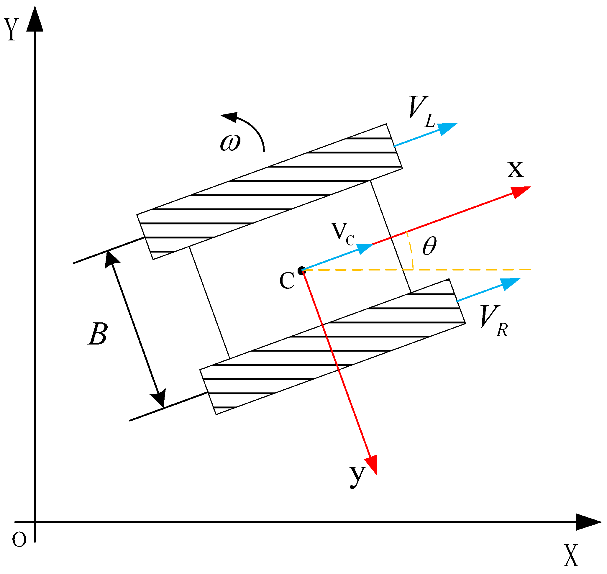
By analyzing the locomotion mechanism of a single-track vehicle, it is observed that during steering, the track on the braked side remains stationary, while the track on the unbraked side drives the vehicle to rotate. The turning center is located at the contact point of the braked track. This motion behavior can be simplified as a classical differential-drive system.

To facilitate kinematic modeling, the following assumptions are made in this study:

• The vehicle moves on a planar (two-dimensional) surface, with the vertical displacement neglected.
• The contact between the tracks and the ground is uniform, and no slippage occurs.
• The center of mass coincides with the geometric center of the vehicle.

Based on these assumptions, a kinematic model of the tracked vehicle is established in the navigation coordinate frame XOY, as illustrated in Figure 3.

To enhance clarity, the definitions of the key symbols used in this model are summarized in

Table 2. Description of the key symbols in the kinematic model.

Symbol	Description
(X, O, Y)	Global coordinate system fixed to the ground, used as the reference frame.
(x, C, y)	Vehicle coordinate system with origin at the center of mass.
C	Position of the vehicle’s center of mass.
B	Distance between the centers of the two tracks (in m).
VR	Velocity of the right track (in m·s−1).
VL	Velocity of the left track (in m·s−1).
VC	Velocity of the vehicle’s center of mass (in m·s−1).
θ	Angle between the vehicle’s x-axis and the global X-axis (rad), positive in the counterclockwise direction.
ω	Angular velocity of the vehicle around its center (in rad·s−1).

below.

According to the kinematic equations of the tracked vehicle, the following can be derived:

$$\left\{\begin{array}{c}\stackrel{·}{x}=V_C·\cos \theta \\ \stackrel{·}{y}=V_C·\sin \theta \\ \stackrel{·}{\theta }=\omega \end{array}\right.$$

(1)

The forward velocity V_C of the vehicle, defined as the linear velocity of the vehicle’s center of mass in the forward direction, is given as the average velocity of the two tracks:

$$V_C={\displaystyle \frac{V_R+V_L}{2}}$$

(2)

When the vehicle turns by braking one track, the angular velocity ω and turning radius R are determined by the track width B and the velocity difference between the two tracks. The turning center is located at the midpoint of the braked track:

$$R={\displaystyle \frac{{\mathrm{V}}_{\mathrm{C}}}{\omega }}={\displaystyle \frac{(V_L+V_R)B}{2(V_L-V_R)}}={\displaystyle \frac{B}{2}}$$

(3)

$$\omega ={\displaystyle \frac{V_R-V_L}{B}}$$

(4)

When the vehicle turns left, the left track is braked, i.e., V_L = 0, then:

$$\left\{\begin{array}{l}{\mathrm{V}}_{\mathrm{C}}={\displaystyle \frac{V_R+0}{2}}={\displaystyle \frac{V_R}{2}}\\ \omega ={\displaystyle \frac{V_R-0}{B}}={\displaystyle \frac{V_R}{B}}\end{array}\right.$$

(5)

When the vehicle turns right, the right track is braked, i.e., V_R = 0, then:

$$\left\{\begin{array}{l}{\mathrm{V}}_{\mathrm{C}}={\displaystyle \frac{V_L+0}{2}}={\displaystyle \frac{V_L}{2}}\\ \omega ={\displaystyle \frac{0-V_L}{B}}=-{\displaystyle \frac{V_L}{B}}\end{array}\right.$$

(6)

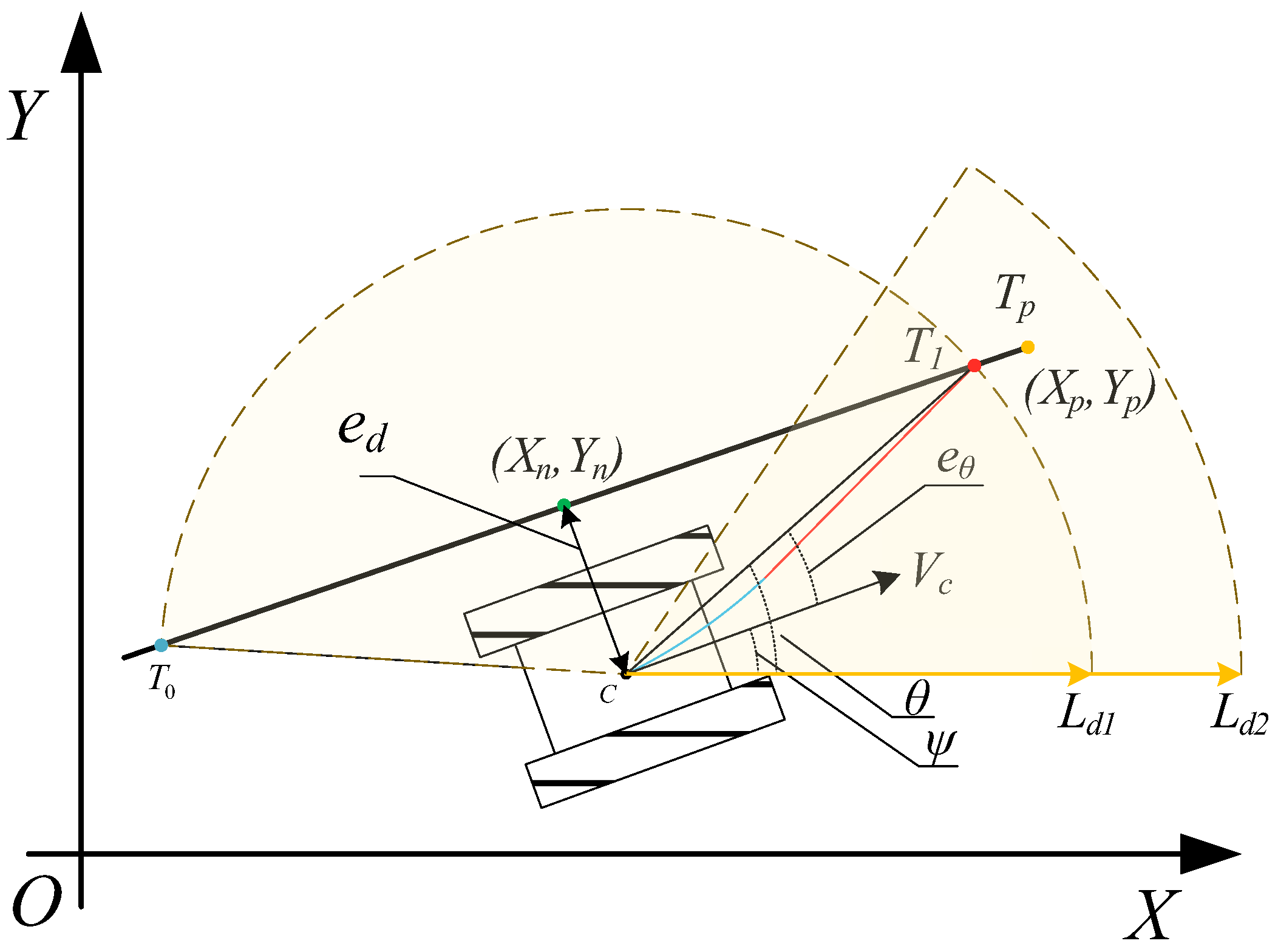
3.2. Segmented Preview Tracking Model

This study adopts a segmented preview tracking model, which divides the path tracking process into two stages: “steering adjustment” and “straight-line motion” (as shown in Figure 4), in order to accommodate the structural characteristic of fixed turning radius in single-track vehicles. The vehicle first utilizes its single-side braking steering mechanism to adjust its heading by calculating the heading deviation and determining the required turning angle, thereby aligning the vehicle toward the preview point. Subsequently, the vehicle moves along a straight path toward the preview point. Upon reaching it, the next preview point is computed and selected, and the process is repeated until the entire path is successfully tracked.

To realize path tracking control, it is necessary to perform real-time computation and updating of key parameters throughout the tracking process. The lateral deviation e_d represents the perpendicular distance between the vehicle’s current position and the target path, indicating the extent of lateral offset. To ensure computational accuracy, the lateral deviation is calculated based on the local direction of the path. By identifying the nearest index point (X_n, Y_n), the corresponding path segment (e.g., from (X_n−1, Y_n−1) to (X_n+1, Y_n+1)) is obtained, and the tangent direction of the path is calculated accordingly:

$${\theta }_{\mathrm{p}}=arctan2(Y_{\mathrm{n}+1}-Y_{\mathrm{n}-1},X_{\mathrm{n}+1}-X_{\mathrm{n}-1})$$

(7)

where θ_p denotes the local heading angle of the path.

Subsequently, the vehicle position vector $\overrightarrow{P}=\left(X-X_n, Y-Y_n\right)$ is projected onto the direction perpendicular to the path, and the lateral error of the vehicle is calculated as follows:

$$e_d=(X-X_n)sin{\theta }_{\mathrm{p}}-(Y-Y_n)cos{\theta }_p$$

(8)

Note: the sign of ed indicates the vehicle’s relative position with respect to the path; e_d > 0 means that the vehicle is on the left side of the path, while e_d < 0 means that it is on the right side.

The current preview point of the vehicle is determined based on the preview distance by calculating the Euclidean distance between the vehicle’s current position and the path points and searching for the point whose distance equals or is closest to the preview distance. However, the vehicle may sometimes select a point located behind its current position as the preview point (e.g., selecting point T₀ in Figure 4), which can lead to path tracking failure. Therefore, a forward-looking constraint must be introduced to ensure that the vehicle progresses along the forward direction of the path. Assuming the path consists of discrete points {(X_i, Y_i)} for i = 0, 1, 2, ⋯, N, a forward constraint is first imposed as follows:

• Find the nearest index point (X_n, Y_n) relative to the vehicle. Compute the Euclidean distance d_i between the vehicle’s current position (X, Y) and each path point.

$$d_{\mathrm{i}}=\sqrt{{(X_{\mathrm{i}}-X)}^2+{(Y_{\mathrm{i}}-Y)}^2}$$

(9)

2.

Identify the point corresponding to the minimum d_i as the nearest index point (X_n, Y_n), with the index value n (i.e., d_n = min(d_i)).

3.

Select the path point that satisfies the preview distance constraint while ensuring that its index satisfies I > n, thereby guaranteeing that the preview point is located ahead of the vehicle. The resulting point is defined as the current preview point.

Meanwhile, to ensure complete path tracking and avoid failures in the final segment caused by the inability to locate a preview point (i.e., (d_i < L_d2)), it is necessary to assign the endpoint of the planned path as the preview point when it falls within the current preview distance. In such cases, the endpoint T_p is taken as the vehicle’s preview tracking point, thereby ensuring complete path coverage.

After determining the preview point, the current heading deviation e_θ of the vehicle is calculated to guide the steering adjustment. The target heading angle θ is computed based on the vehicle’s current position (X, Y) and the coordinates of the preview point (X_T, Y_T) as follows:

$$\theta =arctan2({\mathrm{Y}}_T-Y,{\mathrm{X}}_T-X)$$

(10)

The heading deviation e_θ is defined as the difference between the target heading angle θ and the current heading angle ψ:

$$e_{\theta }=\theta -\psi$$

(11)

To avoid angular discontinuity, e_θ should be normalized to the interval [−π, π].

$$e_{\theta }=atan2(sin(\theta -\psi ),cos(\theta -\psi ))$$

(12)

Note: e_θ > 0 indicates that the vehicle needs to turn left, while e_θ < 0 indicates a right turn.

To provide a quantitative measure of the dynamic characteristics of the path, the average curvature of the forward path (within the preview range) is calculated. The path curvature k represents the degree of bending of the path and is mathematically defined as the rate of change of the tangent angle with respect to arc length at a given point on the curve. For circular arcs, where the curvature is constant, the curvature k is given by the following:

$$k={\displaystyle \frac{\delta }{s}}$$

(13)

Here, δ represents the central angle corresponding to the arc, and s is the arc length of the arc.

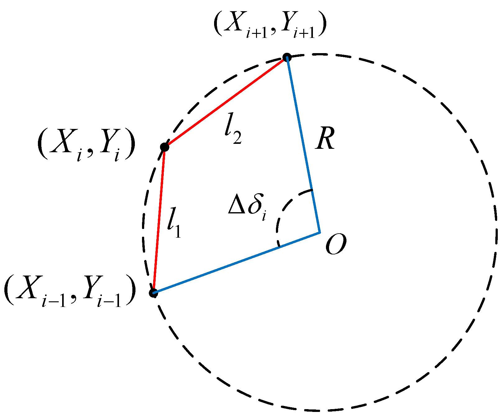
From the nearest point (X_n, Y_n) of the vehicle, a set of points within the preview distance L_d is selected along the direction of the path, denoted as (X_n+1, Y_n+1), …, (X_n+m, Y_n+m), where m is determined by the preview distance L_d. The curvature at each point on the path is estimated using the three-point method. As shown in Figure 5, three consecutive points (X_i−1, Y_i−1), (X_i, Y_i), and (X_i+1, Y_i+1) are selected. The central angle Δδ_i is approximated by the included angle between the two line segments:

$$\Delta {\delta }_i=arccos({\displaystyle \frac{\overrightarrow{v_1}\cdot \overrightarrow{v_2}}{\left|\overrightarrow{v_1}\right|\left|\overrightarrow{v_2}\right|}})$$

(14)

where $\overrightarrow{v_1}=(X_i-X_{i-1},{ Y}_i-Y_{i-1})$, $\overrightarrow{v_2}=(X_{i+1}-X_i,Y_{i+1}-Y_i)$

The arc length Δs_i is approximated based on the three-point arc assumption by taking the average of the lengths of the two segments:

$$\Delta s_i={\displaystyle \frac{\sqrt{{(X_i-X_{i-1})}^2+{(Y_i-Y_{i-1})}^2}+\sqrt{{(X_{i+1}-X_i)}^2+{(Y_{i+1}-Y)}^2}}{2}}$$

(15)

This approximation originates from a geometric simplification in curvature calculations. For a circular arc formed by three points, the true arc length is Δs_i = R·|Δδ_i|, where R is the arc radius. However, calculating R is computationally complex and difficult to obtain in real time. Therefore, the average of the two segment lengths, l₁ and l₂, is used to approximate the arc length. The resulting error is negligible for small angles, ensuring a balance between real-time performance and accuracy.

The curvature at a single point is given by the following:

$$k_{\mathrm{i}}={\displaystyle \frac{|\Delta {\delta }_i|}{\Delta s_i}}$$

(16)

The average curvature is calculated over the m points ahead as follows:

$$k={\displaystyle \frac{1}{m}}{\displaystyle \sum _{i=n}^{n+m-1}{k}_i}$$

(17)

To facilitate the interpretation of Figure 4, a summary of the associated variables and their definitions is provided in

Table 3. Symbol definitions related to the segmented preview tracking model in Figure 4.

Symbol	Description
(X, O, Y)	Global coordinate system fixed to the ground.
Ld1, Ld2	Preview distances (in m).
C	Center of mass of the vehicle.
Vc	Velocity direction of the center of mass (in m·s−1).
T1	Preview point of the tracked vehicle.
Tp	Endpoint of the path.
T0	Point located behind the vehicle.
ed	Lateral deviation of the vehicle (in m).
θ	Target heading angle (in rad).
ψ	Current heading angle of the vehicle (in rad).
eθ	Heading deviation (in rad).
blue line	Tracked vehicle’s turning trajectory.
red line	Straight-line tracking trajectory.
(Xn, Yn)	Point on the path closest to the vehicle.

.

3.3. Dynamic Adjustment Strategy for Preview Distance

In the preview tracking algorithm for tracked vehicles, the preview distance L_d is a key parameter that determines path tracking performance and turning behavior. However, a fixed preview distance often results in frequent turning or excessive tracking deviation under specific conditions, thereby affecting the smoothness of navigation and operational efficiency.

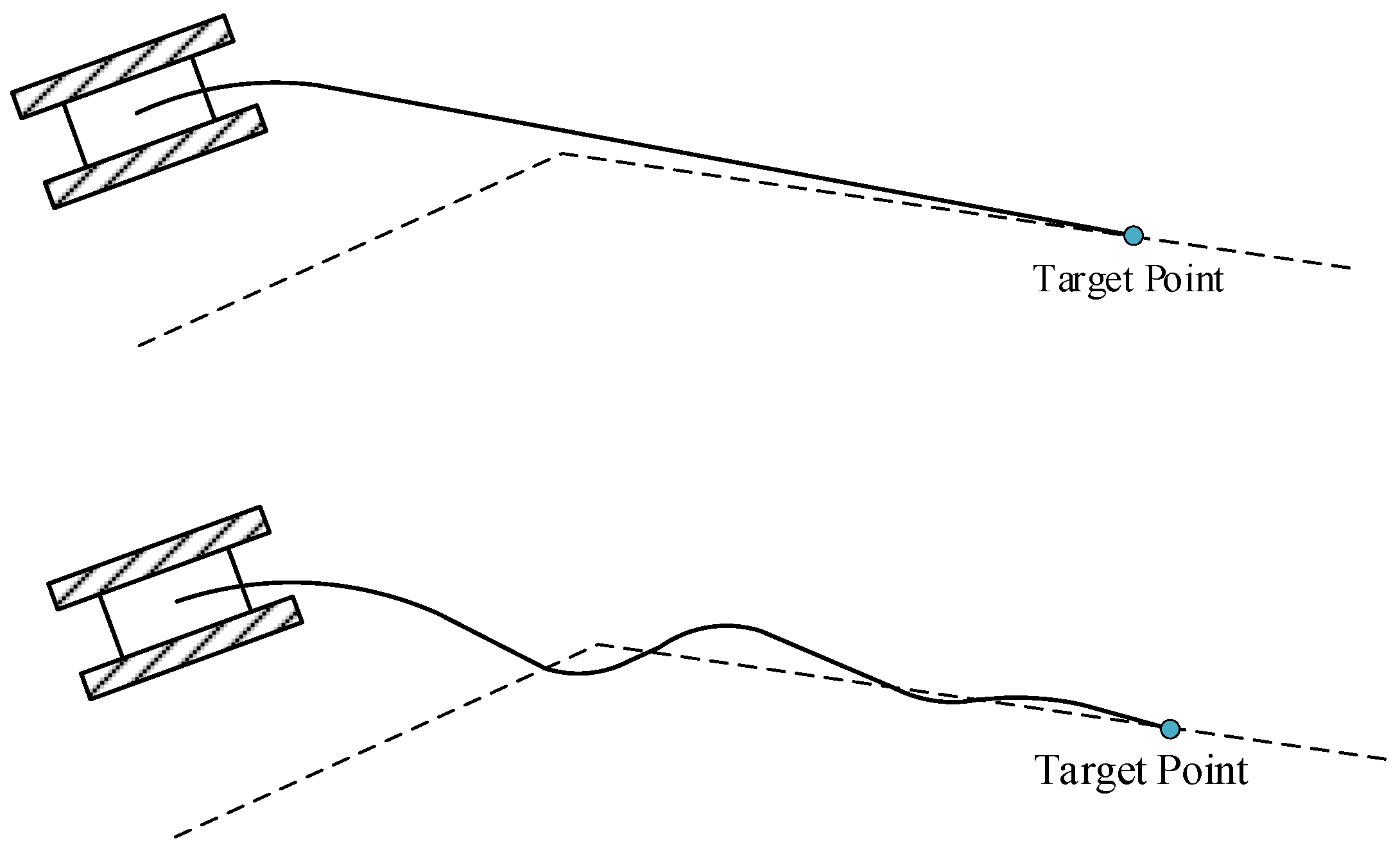
As shown in Figure 6, using a large preview distance may cause the vehicle to skip certain path segments, leading to path tracking failure. Conversely, a small preview distance can cause the vehicle to oscillate back and forth near the reference path. Therefore, to enhance the effectiveness of the preview tracking algorithm, it is essential to dynamically select an appropriate preview distance based on road information and vehicle state.

To ensure stable path tracking, the selection of the preview distance must also guarantee the stability of the tracking system [21]. When the reference path is fully followed, the system must remain in a stable state. The local stability of the nonlinear system under equilibrium conditions can be analyzed by linearizing the system around the equilibrium point.

Based on the geometric preview control model for tracked vehicles, the evolution of lateral error and heading error over time can be described by the following kinematic relationships:

$$\left\{\begin{array}{c}{\stackrel{·}{e}}_d=-v·e_{\theta }\\ {\stackrel{·}{e}}_{\theta }=v·\gamma \end{array}\right.$$

(18)

where e_d is the lateral deviation, e_θ is the heading deviation, v is the vehicle speed, T is the time constant, and γ is the vehicle rotation angle.

To ensure closed-loop stability, the controller applies a dynamic regulation rate to adjust γ based on the observed tracking errors. The adopted regulation law is given as follows:

$$\stackrel{·}{\gamma }={\displaystyle \frac{1}{T}}({\varphi }_{e_{\theta }}\cdot e_d+{\varphi }_{e_d}\cdot e_{\theta }+{\varphi }_{\gamma }\cdot \gamma -\gamma )$$

(19)

where Φ_eθ, Φ_ed, and Φ_γ are the linearization coefficients of the path tracking system.

Combining the above expressions, the closed-loop state-space system can be written as follows:

$$\left[\begin{array}{l}\stackrel{·}{e_d}\\ \stackrel{·}{e_{\theta }}\\ \stackrel{·}{\gamma }\end{array}\right]=\left[\begin{array}{ccc}0& -v& 0\\ 0& 0& v\\ {\displaystyle \frac{1}{T}}{\varphi }_{e_{\theta }}& {\displaystyle \frac{1}{T}}{\varphi }_{e_d}& {\displaystyle \frac{1}{T}}({\varphi }_{\gamma }-1)\end{array}\right]\left[\begin{array}{l}{e}_d\\ e_{\theta }\\ \gamma \end{array}\right]$$

(20)

The characteristic polynomial of the system is calculated as follows:

$$f(\lambda )={\lambda }^3-{\displaystyle \frac{1}{T}}({\varphi }_{\gamma }-1){\lambda }^2-{\displaystyle \frac{v}{T}}{\varphi }_{e_{\theta }}\lambda +{\displaystyle \frac{v^2}{T}}{\varphi }_{e_d}$$

(21)

Based on the Routh–Hurwitz stability criterion, the stability conditions of the system can be obtained as follows:

$$\left\{\begin{array}{l}{\varphi }_{\gamma }-1\le 0\\ {\varphi }_{e_{\theta }}\le 0\\ -({\varphi }_{\gamma }-1){\varphi }_{e_{\theta }}+Tv{\varphi }_{e_d}\le 0\end{array}\right.$$

(22)

If the above conditions are satisfied, the system is locally stable at the equilibrium point. Based on the stability conditions, the following expression is derived:

$$L_d\ge Tv$$

(23)

where L_d is the preview distance, T is the system response time, and v is the vehicle speed.

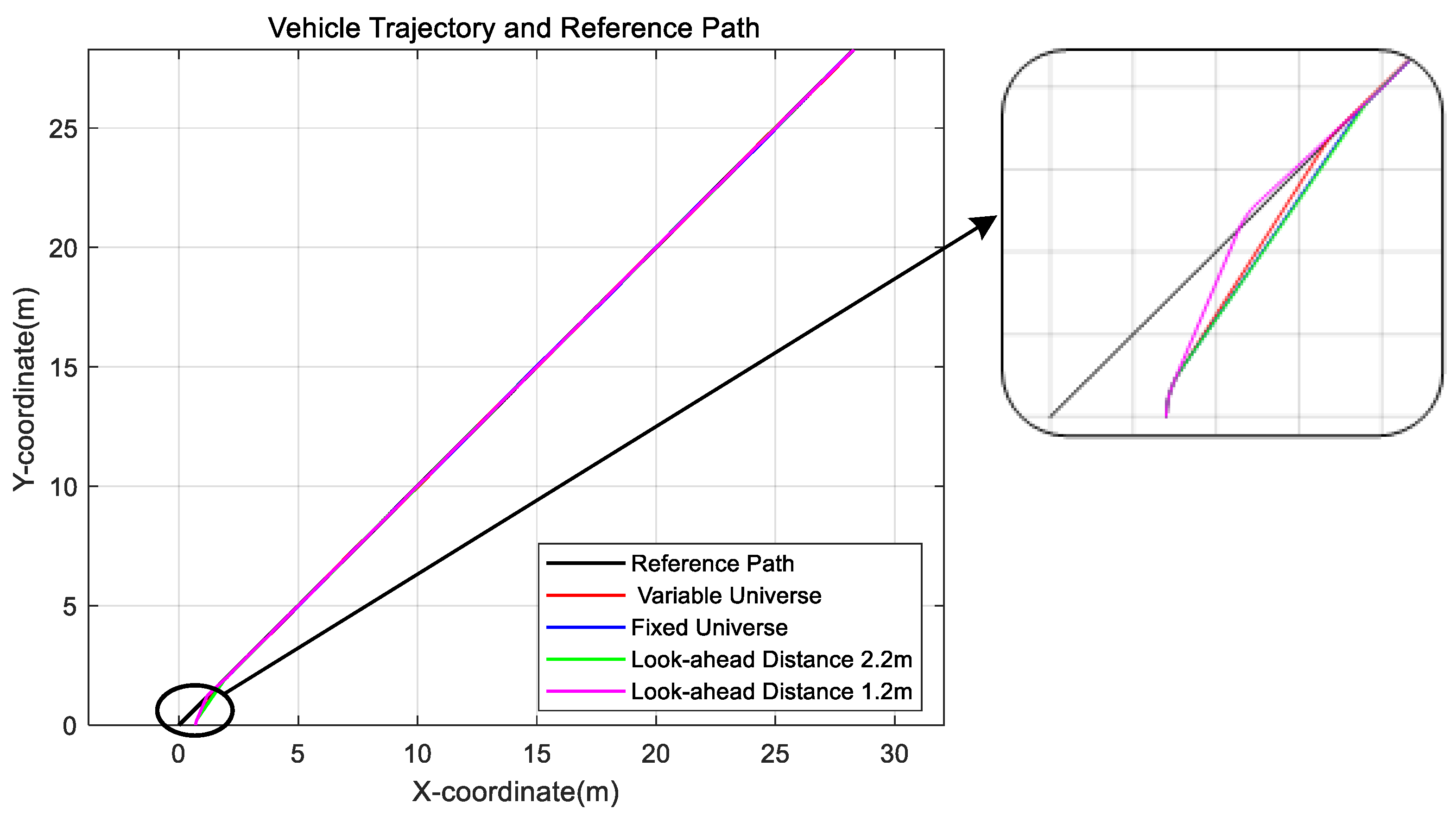
Through experimental analysis, the system response time of the vehicle was determined to be 0.6 s, and the vehicle speed was set to 2 m/s. As a result, the minimum preview distance was calculated to be 1.2 m, indicating that the system can remain stable when the preview distance satisfies L_d > 1.2 m.

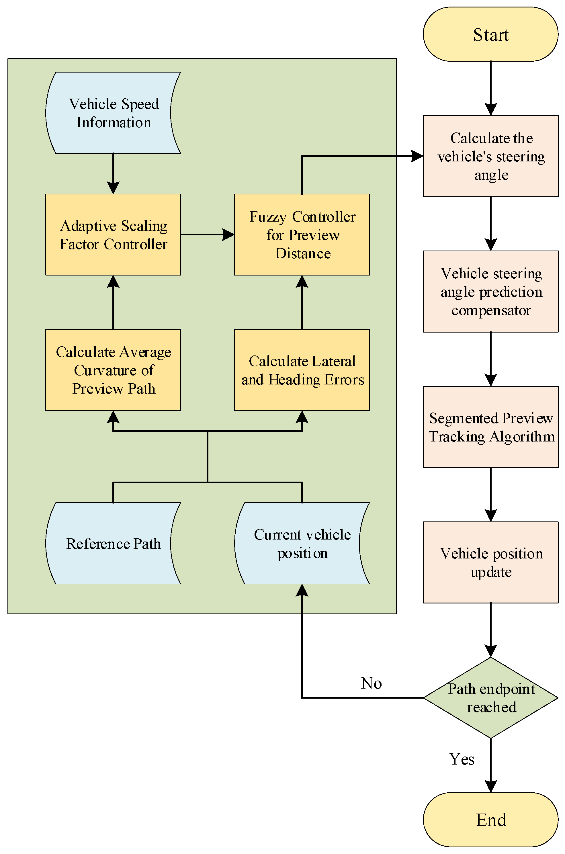
Secondly, this study designs a preview distance adjustment controller based on variable universe fuzzy control. The controller takes the average curvature k of the forward path and the vehicle speed v at a given moment as inputs to an adaptive scaling factor module, which calculates and outputs a universe scaling factor α. Subsequently, the variable universe fuzzy control module adjusts the input universe based on α and performs inference using the current lateral deviation and heading deviation to obtain the optimal preview distance at that moment. Finally, the calculated preview distance is passed into the segmented preview tracking module, which, together with the vehicle’s steering angle prediction compensator, achieves path tracking control.

The algorithm implementation flowchart is shown in Figure 7. The functions and roles of the key modules involved in the control algorithm, as shown in Figure 7, are summarized in

Table 4. Functional descriptions of modules used in the control algorithm (Figure 7).

Module/Block	Description
Vehicle Speed Information	Provides the vehicle’s current speed for use in adaptive scaling.
Adaptive Scaling Factor Controller	Computes the scaling factor based on average path curvature and speed.
Fuzzy Controller for Preview Distance	Infers optimal preview distance using lateral and heading errors.
PSO-SVR Steering Angle Compensator	Predicts and corrects heading deviation to improve steering accuracy.
Segmented Preview Tracking Algorithm	Computes the target heading and guides vehicle movement.
Vehicle Position Update	Updates vehicle state based on GNSS/IMU feedback and trajectory execution.

.

3.3.1. Design of the Variable Universe Fuzzy Controller

The essence of the variable universe fuzzy control lies in a dynamically pointwise-converging interpolation method. While keeping the original fuzzy rules of the controller unchanged, it adjusts the scaling factors online, thereby enabling the dynamic modification of the fuzzy universe [21].

For a dual-input single-output fuzzy preview tracking system, let the fuzzy universe of the input variables be defined as follows:

$$\left\{\begin{array}{c}{X}_1=[-E_1,E_1]\\ X_2=[-E_2,E_2]\end{array}\right.$$

(24)

and the fuzzy universe of the output variable as follows:

$$Y=[-U,U]$$

(25)

The adjusted fuzzy universes after applying the scaling factors are given by the following:

$$\left\{\begin{array}{c}{X}_1=[-\alpha E_1,\alpha E_1]\\ X_2=[-\alpha E_2,\alpha E_2]\\ Y=[-\alpha U,\alpha U]\end{array}\right.$$

(26)

where α is the universe scaling factor.

The ranges of the input and output fuzzy universes dynamically contract or expand according to the system’s real-time state, such as the average curvature k of the forward path and the vehicle speed v. Although the total number of fuzzy rules remains unchanged, when the universe contracts, the fuzzy partitions become finer, thereby increasing the number of effective rules and improving the control accuracy. Conversely, when the universe expands, the fuzzy partitions become coarser, reducing the number of effective rules while accommodating other control requirements. This mechanism enables the controller to apply more appropriate fuzzy rules during different control phases, thereby enhancing the system’s adaptability [22,23].

In this study, a dual-input single-output (DISO) fuzzy controller is designed with the objective of enabling the vehicle to follow a predefined trajectory. The initial parameters of the fuzzy controller, including the membership function ranges and rule base, were set based on control experience and standard fuzzy control principles. These parameters were subsequently fine-tuned through offline simulation experiments to enhance the tracking responsiveness and stability of the algorithm under various deviation conditions.

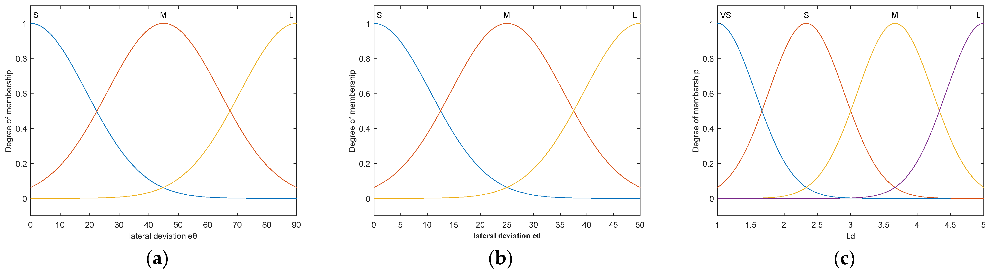
The input variables are the current lateral deviation e_d and the heading deviation e_θ, while the output variable is the preview distance L_d. Since the segmented preview tracking model divides the vehicle tracking into turning and execution phases, and the turning direction can be determined by the sign of the heading deviation, the design of the preview distance focuses more on the magnitude rather than the direction of the input errors. Therefore, the absolute values of the input parameters are used as inputs to the controller.

The basic universe of discourse for the input and output variables is defined as follows: e_d ∈ [0, 50] cm, e_θ ∈ [0, 90]°, and L_d ∈ [1, 5] m. The initial value of the scaling factor is set to 1, with its specific value to be determined through system tuning during operation. 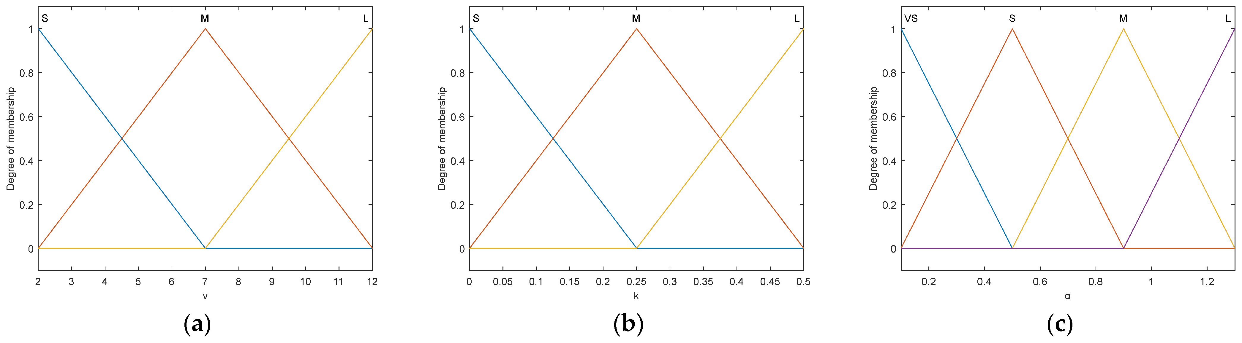The input variables are described using three levels of fuzzy linguistic terms: small (S), medium (M), and large (L); the output variable is defined using four levels: very small (VS), small (S), medium (M), and large (L). To ensure smoothness in the algorithm’s output, all membership functions are modeled using Gaussian membership functions. The membership functions of each variable are shown in Figure 8.

The mathematical expression is given by the following:

$$\mu (x)=e^{-{(x-c)}^2/2{\sigma }^2}$$

(27)

where μ_i is the membership degree, and α_i is the center value of the fuzzy set.

Reasonable fuzzy rules are established as follows: when both e_d and e_θ are large, the preview distance L_d should be reduced to quickly correct the error and improve the tracking accuracy. When e_d and e_θ are small, L_d should be increased to extend the straight-line distance and reduce unnecessary turning. The fuzzy control rules are listed in

Table 5. Variable universe fuzzy control rules.

ed	eθ
	S	M	L
S	L	M	VS
M	M	S	VS
L	VS	VS	VS

.

3.3.2. Design of the Adaptive Scaling Factor

Based on the concept of a variable universe, it is necessary to design a reasonable and effective scaling factor. Existing studies commonly adopt mathematical functions to compute the scaling factor, where its magnitude directly depends on the input variables. These function-based approaches have explicit mathematical models, allowing for fast computation and implementation within control systems. However, such methods often rely on empirically defined parameters [24], which are difficult to tune. Moreover, fixed mathematical formulations cannot fully capture the nonlinear and variable characteristics of complex systems, thereby affecting control accuracy. As a result, they may perform poorly under the diverse operating conditions of agricultural machinery. To enhance the adaptability of the system, this study adopts a fuzzy control approach for scaling factor adjustment. By applying fuzzy inference, the scaling factor is dynamically adjusted in real time based on the average curvature of the path ahead and the vehicle speed. This allows the fuzzy universe to contract more quickly when errors are large—thereby improving the system’s responsiveness—and to expand when errors are small, reducing unnecessary turns and improving the system’s stability.

The adaptive scaling factor controller is designed as a dual-input single-output fuzzy controller. The input variables are the average curvature k of the forward path and the vehicle speed v, while the output variable is the scaling factor α. The adaptive scaling factor controller consists of the following three main steps:

(1) Fuzzification. The fuzzy universe of input variable k is set to [0, 0.5] m⁻¹, and the fuzzy range of vehicle speed v is defined as [2, 12] km/h. Both input variables adopt three levels of fuzzy linguistic terms: small (S), medium (M), and large (L). The fuzzy universe of the output variable α is set to [0.1, 1.3], with four fuzzy linguistic terms: very small (VS), small (S), medium (M), and large (L). The membership functions of both input and output variables use triangular functions, which are computationally simple and suitable for real-time control. The general form is as follows: (μ(x) = max(0, 1 − |x − c|/b)), where c is the center, and b is the width. The membership functions are illustrated in Figure 9.

(2) Establishment of the fuzzy rule base. The design principle of the fuzzy rules for the adaptive scaling factor is as follows: When both k and v are large, a smaller scaling factor is applied to compress the universe, increase sensitivity to errors, and enhance the path tracking capability. When both k and v are small, a larger scaling factor (close to or slightly greater than 1) is used to appropriately expand the universe, reducing excessive adjustments and improving smoothness. When k is large but v is small, a moderately small scaling factor is used to improve the tracking accuracy while avoiding unnecessary sharp corrections. When k is small but v is large, a moderately large scaling factor is adopted to enhance the vehicle stability while maintaining the required tracking precision. The designed fuzzy rule base is shown in

Table 6. Fuzzy control rule table for the universe scaling factor.

K	V
	S	M	L
S	L	L	M
M	S	S	VS
L	VS	VS	VS

.

(3) Defuzzification and fuzzy inference. Fuzzy inference is performed using the Mamdani method. Based on the membership degrees of inputs k and v, the fuzzy rule base is used to compute the fuzzy output of α. The fuzzy output is then defuzzified using the centroid method to obtain a crisp value, calculated as follows: $\alpha =\sum ({\mu }_i·{\alpha }_i)/\sum {\mu }_i$, where μ_i is the membership degree, and α_i is the center value of the fuzzy set. Finally, the computed scaling factor is fed into the variable universe fuzzy controller and applied in the calculation of the vehicle’s preview distance.

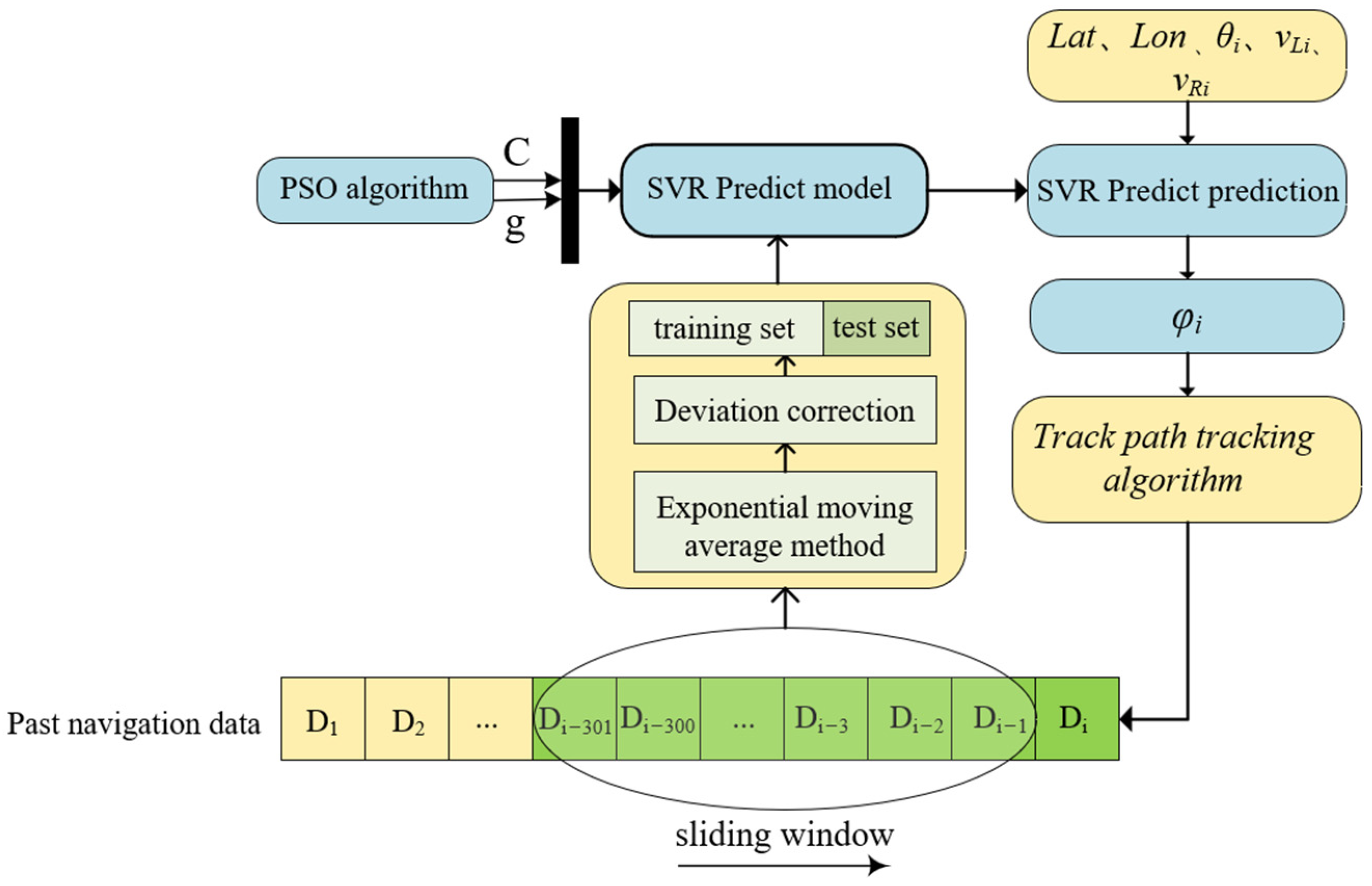
3.4. Vehicle Steering Angle Prediction and Compensation Based on SVR and PSO

Heading deviation refers to the difference between the current heading of the vehicle and the desired heading, which determines the vehicle’s turning direction and turning angle. In practical applications, however, due to factors such as muddy terrain and track slippage, the actual angular velocity during single-track steering tends to be discrete or exhibit nonlinear jumps. As a result, the control process shows discontinuous steering behavior, making it difficult to achieve precise control. This often leads to steady-state errors and an inability to maintain low lateral deviation [25]. Therefore, it is necessary to predict the vehicle’s heading deviation and compensate for the steering angle accordingly so that the vehicle can advance or delay steering actions as needed. Given the highly nonlinear disturbances present in complex farmland environments, it is challenging to develop an accurate model to estimate the actual heading deviation error. In this context, machine learning offers a feasible solution.

Support Vector Regression (SVR), as a nonlinear regression model based on the principle of structural risk minimization, demonstrates strong fitting capabilities for small-sample and high-dimensional data [26]. It can analyze and learn from actual observational data to infer and predict the vehicle’s state at the next moment. Based on the prediction results, compensation can be applied to certain parameter values to achieve more accurate tracking. Therefore, this study adopts the SVR algorithm to predict the vehicle’s heading at the next time step in real time based on the current heading deviation.

During navigation, due to muddy and uneven terrain, the vehicle’s navigation data D (including current GPS coordinates, heading angle, and track speed) exhibit continuous fluctuations, containing both sudden changes and noise. To mitigate the impact of noise and abrupt variations, this study employs the exponential moving average (EMA) method:

$$D_i=\left\{\begin{array}{ll}0& i=0\\ \beta D_{i-1}-(1-\beta ){\theta }_i& i\ge 1\end{array}\right.$$

(28)

where β is the weighting coefficient, which is set to 0.6 in order to enhance the stability of the algorithm and better handle sudden changes. D_i denotes the exponential moving average of the i-th sample, and θ_i represents the original value of the i-th sample. Each round of exponential smoothing is performed using 300 consecutive sampling points.

Considering that the exponential moving average may misestimate the true value due to insufficient initial data, resulting in a systematic bias, a bias correction formula is introduced for compensation:

$$D_i={\displaystyle \frac{D_i}{1-{\beta }^{\mathrm{i}}}}$$

(29)

SVR can be used to construct a nonlinear mapping relationship between input and output variables. Unlike traditional regression methods, SVR maps input samples into a high-dimensional space using a kernel function and determines the regression hyperplane based on the support vectors [27]. Its mathematical expression is given as follows:

$$f(x)={\displaystyle \sum _{i=1}^m({\stackrel{\wedge }{\alpha }}_i-{\alpha }_i)}\cdot k(x_i,x_j)+b$$

(30)

where $k\left(x_i,x_j\right)=\Phi {\left(x_i\right)}^T\Phi \left(x_i\right)$ is the kernel function.

During navigation, the 300 most recent navigation data points are processed using exponential moving averaging. The first 70% of the smoothed results are used as the training set, and the remaining 30% as the test set. The input features include vehicle position information, heading deviation, lateral deviation, and vehicle speed. The target output is the predicted heading deviation, which is used to guide steering control. To avoid falling into local optima and to improve the performance of the SVR model, this study introduces the Particle Swarm Optimization (PSO) algorithm to automatically optimize the key SVR parameters, including the penalty coefficient C and the kernel parameter g. In the PSO algorithm, each particle represents a candidate parameter pair (C, g), where C ∈ [0.1, 100] and g ∈ [0.1, 100]. The mean squared error (MSE) of the SVR is adopted as the fitness function in PSO, and the fitness of each particle is evaluated through cross-validation errors.

PSO dynamically updates each particle’s velocity and position by referring to its own historical best position and the current global best position of the entire swarm [28,29]. Through multiple iterations, the algorithm converges to an optimal set of parameters that minimizes the prediction error of the SVR model, thereby improving its prediction accuracy and generalization capability. In this study, the PSO hyperparameters—including population size, inertia weight, and learning factors—are empirically set to achieve a good balance between convergence speed and prediction performance.

The equations for updating the particle velocity and position are as follows:

$$\left\{\begin{array}{c}{v}_{i,d}(t+1)=\omega v_i+c_1{r}_1(P_{i,d}-x_{i,d}(t))+c_2{r}_2(P_{g,d}-x_{i,d}(t))\\ x_{i,d}(t+1)=x_{i,d}(t)+v_{i,d}(t+1)\end{array}\right.$$

(31)

Note: i is the index of the particle; t is the current iteration number; d is the dimension index of the search space (i.e., the d-th parameter); v_i,d(t) is the velocity of particle i in dimension d at iteration t; x_i,d(t) is the position (i.e., parameter value) of particle i in dimension d at iteration t; P_i,d is the historical best position of particle i in dimension d; P_g,d is the global best position found so far in dimension d; ω is the inertia weight, set to 1; c₁ and c₂ are learning factors, set to 1.5 and 1.7, respectively; and r₁ and r₂ are random numbers uniformly distributed in the interval [0, 1].

After training is completed, new navigation data are input into the trained SVR model, which uses the learned weights and bias to compute the predicted heading deviation of the vehicle. For clarity of representation, the heading deviation is denoted as φ.

To improve the prediction accuracy, this study employs the Mean Bias Error (MBE) to correct the prediction results. MBE measures the average deviation between the predicted heading deviation and the actual heading deviation. The calculation formula is as follows:

$$MBE={\displaystyle \frac{1}{n}}{\displaystyle \sum _{i=1}^n({\phi }_{{\alpha }_i}-{\phi }_{p_i})}$$

(32)

The predicted heading deviation after MBE correction is denoted as ${\phi }_{p_i}^{\prime }$, and its calculation formula is as follows:

$${\phi }_{p_i}^{\prime }=MBE+{\phi }_{p_i}$$

(33)

To further compensate for the heading deviation, a deviation compensation coefficient μ_ci is defined, and its expression is given as follows:

$${\mu }_{ci}={\displaystyle \frac{{\phi }_{e_{i-1}}-{\phi }_{e_i}}{{\phi }_{p_{i-1}}^{\prime }-{\phi }_{p_i}^{\prime }}}={\displaystyle \frac{\Delta {\phi }_e}{\Delta {\phi }_p^{\prime }}}$$

(34)

where φ_e is the expected heading deviation, and ${\phi }_p^{\prime }$ is the MBE-corrected predicted heading deviation.

The prediction error is defined as follows:

$${\phi }_{error,i}={\phi }_{e_i}-{\phi }_{p_i}^{\prime }$$

(35)

The corresponding compensation amount is calculated as follows:

$${\phi }_{c_i}={\mu }_{c_i}\cdot {\phi }_{error,i}$$

(36)

The final actual output heading deviation is as follows:

$${\phi }_i={\phi }_{c_i}+{\mu }_{c_i}\cdot {\phi }_{error,i}$$

(37)

By introducing the heading deviation compensation term to adjust the output of the controller, the heading deviation becomes more consistent with the actual steering behavior of the vehicle, thereby improving the path tracking accuracy of autonomous navigation. The flow of this feedback control algorithm is illustrated in Figure 10.

4. Experiments and Analysis

4.1. Simulation Experiments

To verify the effectiveness of the single-track autonomous navigation system based on variable universe fuzzy control, a simulation platform for single-side braking tracked vehicles was developed using MATLAB 2022b. This platform is used to conduct comparative evaluations against fixed preview distance and fixed-universe fuzzy control methods. In the simulation, the vehicle moves at a constant speed of 2 km/h, with a track width of B = 1 m. The target path is a 40 m straight line oriented at a 45° angle to the x-axis. A comparison of the simulated trajectories is shown in Figure 11, and the corresponding experimental data are provided in

Table 7. Simulation data for path alignment.

Preview Distance (m)/Control Method	Alignment Distance (m)	Number of Turns per Cycle	Average Lateral Error (cm)
2.2	2.0139	18	2.0637
1.2	1.0944	33	1.3160
Fixed-universe fuzzy control algorithm	1.9667	11	2.4727
Variable-universe fuzzy control algorithm (proposed)	1.7111	10	2.7514

.

The distance required for the vehicle to align with the reference path decreases as the preview distance decreases. However, this is accompanied by a significant increase in the number of turns within a control cycle. When the preview distance becomes too small, the vehicle may even deviate beyond the reference path. The algorithm proposed in this study appropriately reduces the fuzzy universe when the initial deviation is large, resulting in more responsive control and a shorter alignment distance. As shown in the table, the alignment distance is reduced by 12.99% compared to fixed-universe fuzzy control, and the number of turns per control cycle is reduced by 9.09%. This demonstrates that the proposed algorithm not only achieves rapid path alignment but also effectively reduces the number of turns during control cycles, thereby enhancing vehicle stability.

Although the proposed algorithm achieves a lower turning frequency, its average lateral error is slightly higher. This is attributed to the control strategy prioritizing rapid alignment in the initial stage while accepting slightly larger oscillations during steady-state tracking. Since the preview distance increases adaptively once the vehicle is aligned, minor lateral deviations tend to persist longer, especially in low-curvature segments. However, the resulting lateral deviation remains within an acceptable range and does not compromise the effectiveness or stability of the control algorithm.

To further verify the adaptability of the proposed path tracking control algorithm under different vehicle speeds and forward path curvature conditions, a test path was designed. The path includes three turning segments with curvatures of 0.2, 0.3, and 0.4, respectively, corresponding to semicircular curves, as well as four straight-line segments, each 40 m in length, simulating various operational conditions. The path tracking result is shown in Figure 12. It can be observed that the variable universe fuzzy control algorithm is capable of dynamically adjusting the preview distance when the path curvature changes, enabling effective path tracking. Compared to the fixed-universe fuzzy control method, the total number of turns over the entire path is reduced by 32.94%, and the average lateral deviation is reduced by 47.11%. Compared to the fixed preview distance method, the total number of turns over the full trajectory is reduced by 20.52%, and the average lateral deviation is reduced by 42.56%. Moreover, no distortion occurs in high-curvature path segments, indicating strong adaptability of the proposed method.

It should be noted that although the Variable Universe Fuzzy Control algorithm may exhibit denser steering actions in curved segments—as visually illustrated in Figure 12—this does not necessarily indicate a higher total number of turns. This phenomenon results from the algorithm’s adaptive behavior: it increases the turning frequency in high-curvature regions to minimize the lateral deviation while reducing unnecessary corrections in straight segments. Consequently, the overall number of turns over the entire trajectory is lower than that of the fixed-universe fuzzy control, as reflected in

Table 8. Comprehensive path simulation data.

Preview Distance/Control Method	Number of Turns	Average Lateral Error (cm)
2.2	85	4.4425
Fixed-universe fuzzy control algorithm	71	3.5682
Variable-universe fuzzy control algorithm (proposed)	57	2.3498

.

4.2. Field Experiments

To further validate the proposed path tracking algorithm, a field test was conducted on an open farmland path. The test site was located at the experimental field of Xihua University in Chengdu, China, with coordinates of longitude 103.9571° and latitude 30.7781°. The operating environment is shown in Figure 13, where uneven terrain and the presence of weeds can be observed. To evaluate the effectiveness of the designed vehicle steering angle prediction compensator, multiple reference points were set along the path. The vehicle was commanded to track these reference points sequentially at a speed of 2 km/h, and a comparative analysis was performed between the cases with and without the prediction compensator enabled. The results showed that the mean absolute heading angle deviation without the compensator was 10.06°, while with the compensator enabled, it was reduced to 3.78°, representing a 32.34% improvement. As illustrated in Figure 14, in the absence of the prediction compensator, the vehicle exhibited significant deviation from the reference points after turning, requiring multiple adjustments to realign with the path. In contrast, when the compensator was activated, the steering control was significantly more accurate, effectively reducing the need for repeated heading adjustments.

In addition, a gradually inward-curving path was designed in the field to verify the adaptability of the proposed path tracking algorithm to curvature variations. The field experiments were conducted to evaluate the overall tracking performance of the proposed algorithm in a continuous and realistic operating environment. To ensure stability and avoid unnecessary disturbances in the experimental data, no artificial lateral offset was introduced at the starting point.

The vehicle was tested three times under each of the three control strategies: variable-universe fuzzy control, fixed-universe fuzzy control, and fixed preview distance. The path tracking result of one representative trial is shown in Figure 15, while the distribution of lateral tracking errors is illustrated in Figure 16. The complete results from the three trials are summarized in

Table 9. Comparison of path tracking performance among different algorithms in three trials.

	Path Tracking Algorithm	Number of Turns per Cycle	Average Lateral Error (m)	Maximum Lateral Error (m)	Standard Deviation of Lateral Error (m)
Trial 1	Variable-universe (proposed)	142	0.0485	0.4266	0.0610
	Fixed-universe	173	0.0840	0.5790	0.0940
	Fixed preview distance	213	0.1070	0.4186	0.0790
Trial 2	Variable-universe (proposed)	153	0.0493	0.5140	0.0592
	Fixed-universe	178	0.0712	0.6584	0.0843
	Fixed preview distance	220	0.0894	0.5136	0.0814
Trial 3	Variable-universe (proposed)	149	0.0516	0.6120	0.0602
	Fixed-universe	191	0.0723	0.5123	0.0927
	Fixed preview distance	205	0.0853	0.4541	0.0876

.

To assess whether the differences in path tracking performance among the control methods were statistically significant, a significance analysis was conducted based on the data from three repeated field trials. One-way ANOVA and pairwise independent-sample t-tests were applied to key performance indicators [30], including the number of turns per control cycle, average lateral deviation, and its standard deviation. The results indicate that the proposed variable-universe fuzzy control method exhibited statistically significant improvements over the other two methods in multiple metrics (p < 0.05), demonstrating its superior tracking performance under complex terrain conditions. Significant differences are marked in

Table 10. Statistical comparison of overall path tracking performance among different algorithms (mean ± SEM).

Path Tracking Algorithm	Number of Turns per Cycle	Average Lateral Error (m)	Standard Deviation of Lateral Error (m)
Variable-universe (proposed)	148 ± 5.5 (*)	0.0498 ± 0.0016 (*)	0.0601 ± 0.0009 (*)
Fixed-universe	181 ± 9.0 (*)	0.0758 ± 0.0071 (*)	0.0903 ± 0.0042 (*)
Fixed preview distance	212 ± 7.6 (*)	0.0939 ± 0.0115 (*)	0.0827 ± 0.0043

Note: (*) indicates that the result differs significantly from other control methods (p < 0.05) based on one-way ANOVA and independent-sample t-tests conducted over three repeated field trials.

using superscript symbols.

Due to the presence of uneven terrain, lateral deviations exhibited some oscillations. However, the proposed algorithm still maintained good stability. As shown in the data in Table 10, the number of turns per control cycle was reduced by 30.19% and 18.23% compared to the fixed preview distance and fixed-universe fuzzy control methods, respectively. The average lateral deviation was reduced by 34.29% and 46.96%, respectively.

5. Discussion

To better clarify the technical innovation and engineering feasibility of this study, a comparative analysis is conducted against representative existing methods, and the applicability of the proposed approach in complex environments is further explored.

Jaramillo-Martínez et al. [31] proposed a reinforcement learning-based path planning method that combines Deep Q-Learning with a Lyapunov-based path tracking controller for autonomous mobile robots (AMRs). This method improves the trajectory smoothness and reduces the number of turns through a carefully designed reward function. Although it performs well in minimizing path length and turning frequency, its heavy reliance on discrete grid modeling and large-scale training iterations limits its adaptability to real-time variations and nonlinear disturbances commonly found in unstructured agricultural environments.

Compared with reinforcement learning-based methods, the approach proposed in this study offers advantages such as interpretable control behavior, high computational efficiency, and deployment-friendliness on embedded platforms. Specifically, the variable universe fuzzy controller adopts Gaussian membership functions and a three-level linguistic classification, maintaining a compact rule base (typically 3 × 3 or 3 × 4). The inference and defuzzification process can be implemented using lookup tables and multiply–accumulate operations, making it well-suited for deployment on low- to mid-end microcontrollers (MCUs) using fixed-point or integer operations. It can operate stably under sampling rates of 100–200 Hz without noticeable delay.

Meanwhile, the SVR-based compensation module adopts a sliding window update strategy with one-step-ahead prediction and offline PSO optimization of parameters, which avoids the need for online kernel learning or complex regression matrix solutions. Once deployed, the model only requires evaluating a small number of kernel functions (e.g., RBF) and computing their linear combination. In our experiments, the input dimension was around 4–5, with fewer than 50 support vectors, and the inference time per prediction was less than 2 ms—demonstrating stable real-time performance on embedded Linux platforms, such as ARM A53. These features make the method particularly suitable for resource-constrained agricultural platforms [32].

Pérez-Juárez et al. [33] developed a fuzzy PID-based trajectory tracking controller for wheeled robots operating in virtual environments. Their fuzzy system symmetrically adjusts PID parameters to achieve good error convergence and control robustness. While this method demonstrates certain adaptive capabilities, it is tailored for continuous control in holonomic systems and is not suitable for the nonholonomic tracked vehicles considered in this study, which use unilateral braking and exhibit a fixed turning radius. To bridge this gap, our work introduces a preview point segmentation model based on tracked vehicle dynamics, along with a PSO-optimized SVR-based yaw compensation strategy that significantly enhances turning accuracy and path tracking continuity.

In addition, considering that agricultural machinery often operates under challenging conditions—such as high travel speeds, steep slopes, loose gravel, and irregular terrain—existing control methods require further improvements in environmental adaptability. At higher speeds, vehicle response delays and increased inertia demand more responsive preview distance estimation and real-time error prediction. Therefore, future work may incorporate speed-segmented control strategies or dynamically weighted fuzzy compensation mechanisms to enhance responsiveness and accuracy under high-speed scenarios.

Furthermore, in environments with severe terrain disturbances—such as loose soil, gravel roads, or inclined fields—tracked vehicles may experience slipping, sinking, or fluctuating traction, which can exacerbate the deviation between the model and actual behavior. To improve the system’s robustness under such conditions, future work can consider integrating multi-source sensor information (e.g., IMU, terrain adhesion estimation), incorporating terrain factors into the fuzzy inference system, or introducing disturbance observers and hybrid neuro-fuzzy networks for real-time modeling and compensation of nonlinear interferences.

Overall, the proposed method has demonstrated strong adaptability and control performance under current speeds and typical hilly terrains. Future extensions toward higher speeds, stronger disturbances, and more diverse field conditions may focus on adaptive fuzzy rule expansion, terrain-aware disturbance modeling, and integration with predictive control to further improve the system’s intelligent decision-making and control capabilities in complex agricultural environments.

6. Conclusions

This study focuses on the path tracking problem of single-track electric agricultural chassis in farmland environments. Based on preview tracking, a variable-universe fuzzy control method was employed to dynamically adjust the preview distance. This approach effectively reduces the number of turns during tracking and enhances the system’s stability. In addition, a vehicle steering angle prediction compensator was developed using a combination of Support Vector Regression (SVR) and Particle Swarm Optimization (PSO), enabling precise control of turning maneuvers for single-track agricultural vehicles and reducing steady-state errors. Comprehensive path tracking experiments were conducted in field conditions. The results showed that, compared with fixed preview distance and fixed-universe fuzzy control methods, the proposed algorithm reduced the average number of turns by 30.19% and 18.23% and decreased the average lateral error by 34.29% and 46.96%, respectively, thus verifying the effectiveness of the proposed approach. The following conclusions are drawn:

(1) A universe scaling factor fuzzy controller and a preview distance fuzzy controller were designed. The average path curvature k and vehicle speed v were used as inputs to compute the universe scaling factor α. The current lateral deviation e_d and heading deviation e_θ were then input into the controller, with the fuzzy universe adjusted dynamically based on α to determine the preview distance L_d. This approach enables the preview distance to be adaptively adjusted according to environmental information, thereby reducing the number of turns per control cycle.

(2) The PSO-SVR method was employed to predict the vehicle’s heading deviation and to compensate for the steering angle, which effectively improved the vehicle’s turning control capability under external environmental disturbances, thereby reducing the path tracking error of agricultural equipment. Additionally, this method enables real-time adjustment based on navigation information, allowing the system to rapidly adapt to different operating environments.

In future work, the proposed algorithm will be further enhanced to improve its adaptability to complex and slippery farmland environments. Additionally, specific issues related to single-track turning—such as severe soil disruption and soil accumulation caused by excessive turning of one track—will be considered in the path tracking algorithm design to improve the environmental adaptability of agricultural equipment.