Article

Maximum Entropy Niche-Based Modeling for Predicting the Potential Suitable Habitats of a Traditional Medicinal Plant (Rheum nanum) in Asia under Climate Change Conditions

1
Humanities and Social Sciences, Jiangsu University of Science and Technology, Zhenjiang 212000, China
2
School of Surveying and Land Information Engineering, Henan Polytechnic University, Jiaozuo 454000, China
3
College of Forestry, Northwest Agriculture and Forestry University, Xianyang 712100, China
4
Institute of Soil and Water Conservation, Chinese Academy of Sciences and Ministry of Water Resources, Xianyang 712100, China
5
Institute of Soil and Water Conservation, Northwest Agriculture and Forestry University, Xianyang 712100, China
*
Author to whom correspondence should be addressed.
These authors contributed equally to this work.
Agriculture 2022, 12(5), 610; https://doi.org/10.3390/agriculture12050610
Submission received: 15 April 2022 / Accepted: 22 April 2022 / Published: 26 April 2022
(This article belongs to the Special Issue Modeling the Adaptations of Agricultural Production to Climate Change)

Abstract

:
Rheum nanum, a perennial herb, is a famous traditional Chinese medicinal plant that has great value in modern medicine. In order to determine the potential distribution of R. nanum in Asia, we specifically developed the potential distribution maps for three periods (current, 2050s: 2041–2060, and 2070s: 2061–2080) using MaxEnt and ArcGIS, and these were based on the current and future climate data under two climate scenarios (RCP2.6 and RCP6.0). To predict the potential impacts of global warming, we measured the area of suitable habitats, habitat suitability changes, and habitat core changes. We found that bio16 (i.e., the precipitation of the wettest quarter) and bio1 (i.e., the annual mean temperature) were the most important climate factors that influenced the distribution of R. nanum. The areas of high suitable habitats (HH) and middle suitable habitats (MH) in the current period were 156,284.7 ± 0.99 km2 and 361,875.0 ± 3.61 km2, respectively. The areas of HH and MH in 2070RCP6.0 were 27,309.0 ± 0.35 km2 and 123,750 ± 2.36 km2, respectively. The ranges of 82.0–90.3° E, 43.8–46.5° N were the mostly degraded areas of the 2050s and 2070s, and RCP6.0 had a larger decrease in habitable area than that found in RCP2.6. All the HH cores shifted south, and the shift distance of HH in 2070RCP6.0 was 115.65 km. This study provides a feasible approach for efficiently utilizing low-number occurrences, and presents an important attempt at predicting the potential distribution of species based on a small sample size. This may improve our understanding of the impacts of global warming on plant distribution and could be useful for relevant agricultural decision-making.

1. Introduction

In China, Rheum L. plants are traditional medicines distributed in the Greater Khingan Range, the Taihang Mountains region, the Qinling Mountains region, the Daba Mountains region, west of the Yunnan–Guizhou Plateau, and the Qinghai-Tibet Plateau [1,2,3]. At present, studies on Rheum L. plants mainly focus on its functional extracts [4,5,6,7,8]. As one of the most heat-tolerant and drought-tolerant species of Rheum L. plants [1], Rheum nanum Siev. ex Pall has been found in Mongolia, Kazakhstan, Russia, and China (i.e., Xinjiang, Gansu, and Inner Mongolia), which mainly inhabit hillsides, valleys, and gravel lands below 1000 m [9]. The latest study showed that chrysophanol, an active constituent of R. nanum, has been effective for obesity and may cure certain skin disorders such as acne vulgaris [10]. Emodin, another active constituent of R. nanum, has suppressed the growth and the invasion of colorectal cancer [11] and has been used to cure acute kidney injury [12]. Previous studies have shown that precipitation and temperature are the dominate factors affecting the geographic distribution of Rheum L. plants [1,3]. R. nanum extracts have played an important role in modern medicine; however, to the best of our knowledge, the exact geographic distribution and the suitable habitats of this ancient medicine remain unexplored.
With the development of computer technology, it has become possible to predict the distribution pattern of the species’ niche by using occurrence data and associated environmental variables [13] with the help of species distribution models (SDMs). According to their dependence of occurrence data, SDMs can be roughly divided in two groups: occurrence-absence data groups (e.g., generalized additive models, generalized linear models, generalized boosting models) and occurrence-data-only groups (e.g., domain model, ecological niche-factor analysis model) [14,15]. The occurrence-data-only models typically have greater advantages as the absence data are usually difficult to collect in the real world, especially for poorly known species [16]. Among various occurrence-data-only SDMs, the maximum entropy model (MaxEnt) [17] has been used extensively because of its strong statistical foundation (i.e., high accuracy and robustness [14,18,19,20,21]) and ability to simulate ecological relationships [22]. Until now, MaxEnt has had a wide range of applications with relevant predictions [23,24,25,26,27,28,29]. Moreover, MaxEnt has better performance for species with a small sample size [16], especially for those species with typically little occurrence records [30].
Over the past 100 years, the global average temperature has risen by 0.6 °C [31,32]. By the end of this century, with a maximum increase of 2.6–4.8 °C in global average temperature [33], global precipitation will increase by approximately 31% [34]. Throughout the evolutionary history of diverse species [31,35], climate change has had significant impacts on the spatial distribution patterns of organisms [32,36]. Global warming has also been confirmed to have the ability to change species’ survival [35] and conservation situations both spatially and temporally [37,38]. With the growing concern of global warming and its potential effects, there have been many useful studies on ecological modeling and conservations using multiple factors and methods [39]. In sub-Saharan Africa, under future climate scenarios, rice production will experience relevant losses in different regions [40]. For alpine plant communities in mountain ecosystems, elevation-dependent warming presents additional challenges and may result in the extinction of cold-adapted flora species [41,42]. In addition, the herbaceous and woody species in mountain basins and the Taklamakan Desert are more sensitive to climate change than plant species in meadows and steppe regions [36]. For Stipa purpurea, a perennial herbaceous plant widespread throughout the Tibetan Plateau, its number of suitable habitats is expected to increase from 1990 to 2050 [27]. Both the herbaceous species and dwarf shrubs will shift upwards in the alpine tundra region of the Changbai Mountains [43]. Hence, it is expected that the possible biogeographic patterns of R. nanum could change with global warming. Based on the effects of increasing temperatures on the global distribution of flora species, we developed two hypotheses: (1) high suitable habitats of R. nanum will increase and move northward; (2) the higher emission scenario may cause a larger increase in the habitat area of R. nanum than the lower emission scenario. The aim of this study was to predict the potential distribution of R. nanum in Asia under climate change and to verify our two hypotheses.

2. Materials and Methods

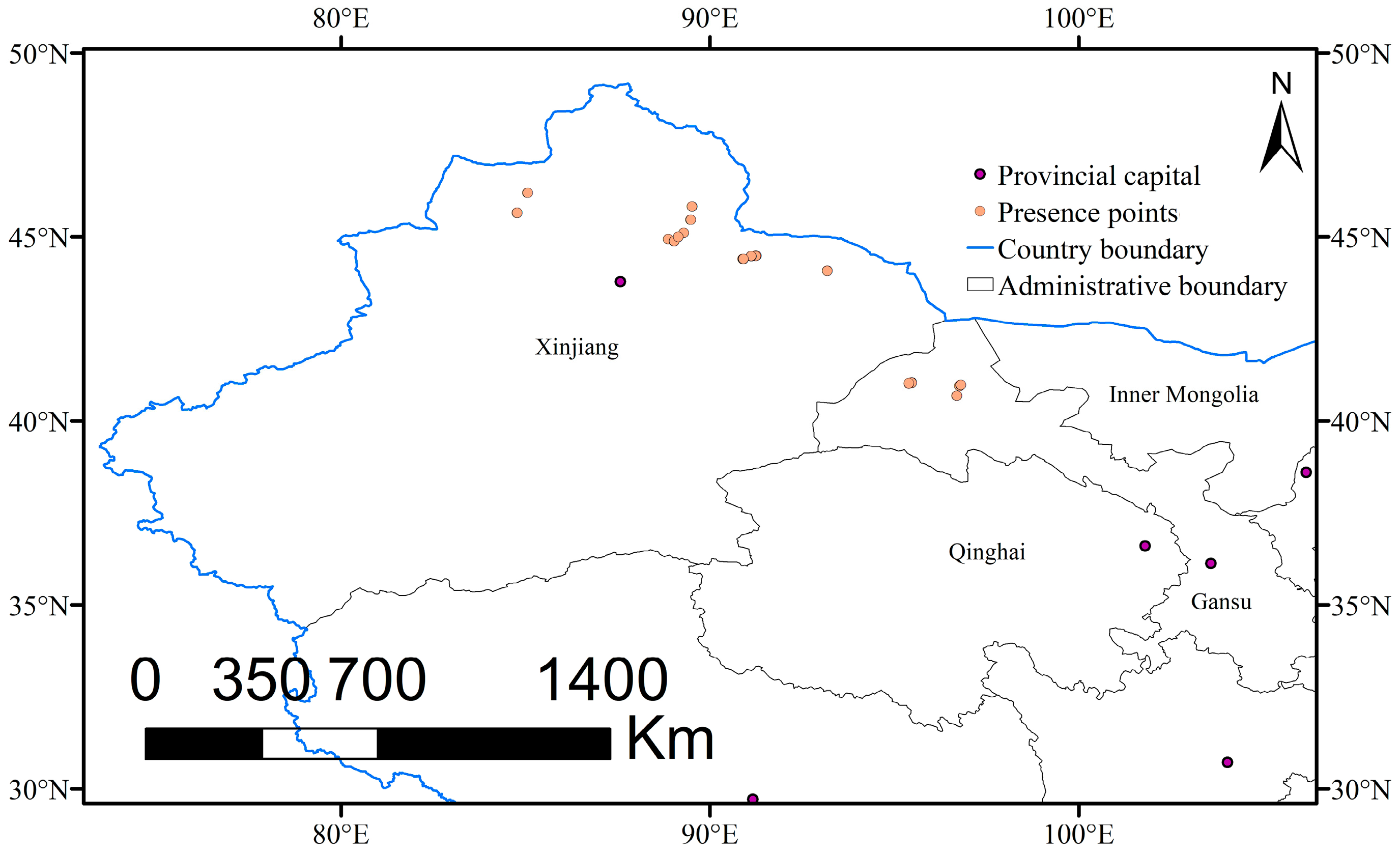
2.1. Occurrence Data and Study Area

The study area range was 70.9–136.5° N, 17.8–55.5° E in Asia. We initially selected 58 region names with relevant habitat descriptions (e.g., text, photo, or GPS points) from online resources (http://www.cvh.ac.cn/ accessed on 21 April 2022, http://www.cfh.ac.cn/ accessed on 21 April 2022 and http://www.plantphoto.cn/ accessed on 29 June 2016) and the published literature [1,3]. At an approximate position, we conducted a two-and-a-half year (2016–2018) field survey in north and northwest China, and collected 246 occurrence data with GPS. To improve the accuracy of prediction and reduce overfitting [44], SDMs toolbox version 2.4 for ArcGIS 10.2 was used to rarefy the occurrence data. Since the resolution of environmental variables used in the MaxEnt model was 2.5 arc-minutes (approximately 5 km), to ensure that each variable grid covered, at most, one occurrence point, we filtered the occurrence data with a buffer distance of 5 km and finally selected 16 occurrence points (Figure 1) for the MaxEnt model. The occurrence points are usually divided into two types according to their usage: the training sample layer and the test sample layer. The rarefied sample size was too small and the widely used method of setting “random test percentages” (i.e., 20–30% of occurrence data [45,46]) would further reduce the sample size. Therefore, to overcome the limitations of a small sample size, we decided to set the 16 occurrence points (i.e., a 5 km buffer) as the training sample layer, and also sought other occurrence points that differed from the training samples as the test sample layer. We rarified the 246 occurrence data again with a 1 km buffer, and then obtained 27 points, which covered the 16 occurrence points (i.e., a 5 km buffer) previously selected. After removing the 16 samples from the 27 newly acquired samples (i.e., a 1 km buffer), we obtained 11 sample points that could be set as the test sample layer for the MaxEnt model.

2.2. Environmental Variables

Nineteen climate variables (2.5 arc-minutes resolution, Table S1) for the current (1970–2000) and future (2050s: 2041–2060 and 2070s: 2061–2080) periods were downloaded from the WorldClim version 1.4 dataset (https://www.worldclim.org accessed on 21 April 2022). The current climate data are interpolations from the observed data, and the future climate data are projections from the Intergovernmental Panel on Climate Change (IPCC [47]) Fifth Assessment Reports (AR5). The future projection data has four “representative concentration pathways” (RCPs. 2.6, 4.5, 6.0, and 8.5 [48]) and examines four possible future radiative forcing levels (2.6, 4.5, 6.0, and 8.5 W/m2 [46]). The emission scenarios consider the potential impacts of policies on future greenhouse gas emissions and provide more scientific descriptions of possible future climate changes [17,49]. Among them, RCP2.6 is the lowest emission scenario (i.e., the most optimistic case) with ~490 parts per million (ppm) CO2 concentrations until 2100, RCP4.5 and RCP6.0 are middle of the road (i.e., the more optimistic case, ~650 ppm and 850 ppm, respectively), and RCP8.5 is the highest emission scenario (i.e., the worst case, ~1370 ppm, https://www.carbonbrief.org accessed on 21 April 2022). RCP2.6 is the only case that could generally limit the global mean temperature increase below 2 °C by 2100 [49], because previous studies have indicated that without proper control, the CO2 concentrations will likely reach 560 ppm (double the pre-industrial level) and 800 ppm by 2060 and 2080, respectively [50]. Hence, in this study, we chose RCP2.6 and RCP6.0 of the Beijing Climate Center–Climate System Model version 1.1 (BCC–CSM 1.1 [51,52]) as the future climate change scenarios.

2.3. Model Processing and Evaluation

For SDMs, rare samples may lead to an imperfect match between the environmental variables and the occurrence data, which brings great difficulties to model evaluation and easily leads to model overfitting [53]. To our knowledge, MaxEnt is one of the few models that perform well in small sample simulations [16,53]. Over the past two decades, MaxEnt, an occurrence-data-only machine-learning program [54], has had extremely extensive procedures on predicting the potential distribution of species [44,55]. Previous studies indicates that 15 might be the minimum number of occurrence points for ecological niche modeling [16]. For Asian species which have >15 available occurrences, the MaxEnt model may provide a broad spectrum of predictions [16]. Moreover, the jackknife test reflects the contributions and the importance of environmental factors in the MaxEnt model [56,57,58]. The area under the curve (AUC) value, based on the receiver-operating characteristic (ROC), ranges from 0 to 1 and reflects the accuracy of the MaxEnt model’s prediction [14,56,59]. Values of 0.8–0.9 indicate a good prediction while values of 0.9–1.0 represent an excellent prediction [17,32,54].
We converted 19 bioclimate environmental variables (bio1–bio19) to ASCII format using Toolbox of ArcGIS 10.2, and then imported the file along with the species occurrence data (in ASCII format) into MaxEnt 3.4.1 for pre-selection. Based on the default settings, we set 16 occurrence data (i.e., at 5 km) as the model training dataset and 11 occurrence data (i.e., at 1 km) as the model testing dataset. A correlation analysis (r > 0.8) was conducted to avoid the potential over-fitting [60,61] of environmental variables, and we obtained two factors (more details in [62]): the annual mean temperature (bio1) and the annual precipitation (bio12). In order to measure the contribution and importance of the 19 variables, we conducted a pre-selection with a set of 1000 iterations, a jackknife test, and an analysis of the response curves, and used default values for other settings. According to the pre-selection result (Table S1), the precipitation of the wettest quarter (bio16) and bio1 contributed to the model the most. Previous studies have indicated that, for Rheum L. plants, seasonal precipitation and relevant temperature during the growth period (March to September [9], and March to May for some species in extreme conditions) are the key factors affecting its spatial distribution [1,2,3]. Hence, after comprehensively considering the results of the correlation analysis, the pre-selection, and the possible environmental needs of R. nanum, we finally chose 6 bioclimatic factors (Table 1) as the environmental layers of the MaxEnt in this study. To improve the projection accuracy and reduce uncertainty, we launched the MaxEnt with the previous settings and ran it 10 times (i.e., 10 “replicates” with basic settings). We calculated the contributions and importance of the 6 factors (Table 1) with Excel and the obtained raster layers in ASCII format were then imported into ArcGIS for further analysis.
We defined the logistic threshold of “balance training omission, predicted area, and threshold value” as TH, and divided the obtained float raster maps into four classes using the reclassify tool [54,55]: UH (unsuitable habitat, 0–TH), LH (low suitable habitat, TH–0.3), MH (middle suitable habitat, 0.3–0.6), and HH (high suitable habitat, 0.6–1.0). The area of suitable habitats as well as habitat maps showing the increases and decreases in habitat range were measured using a raster calculator tool. The cores of habitats and range shifts of habitats were calculated by the zonal geometry (i.e., by calculating the area and centroid of the input raster or feature zone data using a specific zone field, which must be an integer field) and the mean center tool (i.e., by identifying the geographic center for a set of features with case field and weight field, which determine the rank and weight value, respectively; the rank represents the suitability classes, and the weight represents the floating value of MaxEnt.). To quantify the level of increase and decrease in habitat suitability, we defined UH, LH, MH, and HH as 1, 2, 3, and 4, respectively. The raster calculator tool of ArcGIS was used to test and compare the changes in habitat suitability over two periods. The changes in the habitat suitability degree of −1, −2, and −3, respectively, represent a slight, moderate, and dramatic decrease, while +1, +2, and +3, respectively, represent a slight, moderate, and dramatic increase. In addition, we chose the ratio of the area corresponding to the habitat suitability change degree and the total area of suitability change (i.e., increase or decrease) to quantify the changes in habitat suitability.

3. Results

3.1. Contributions and Importance of Environmental Variable in the MaxEnt Model

The mean AUC value of the training data was 0.992 ± 0.003 (Figure S1a), indicating that MaxEnt had excellent prediction performance. The Jackknife importance test showed that the mean value of the regularized training gain of the six factors was 3.127 (Figure S1b,c). When the environmental variables were used in isolation, bio16 (i.e., the precipitation of the wettest quarter) had the highest gain of 1.825, bio1 (i.e., the annual mean temperature) had the second highest gain of 1.455, and bio14 (i.e., the precipitation of the driest month) had the lowest gain of 0.291. Moreover, bio1 (2.751) had the largest decrease in gains when it was omitted, followed by bio16 (3.021) and bio15 (3.047) (Figure S1c).
The MaxEnt model results showed that the variable that contributed the most was bio16 (55.9%), followed by bio1 (13.9%) and bio14 (9.7%); the most important factor in the MaxEnt model was bio1 (54.1%), and the second and third most important factors were bio16 (20.0%) and bio19 (i.e., the precipitation of the coldest quarter, 13.4%), respectively.

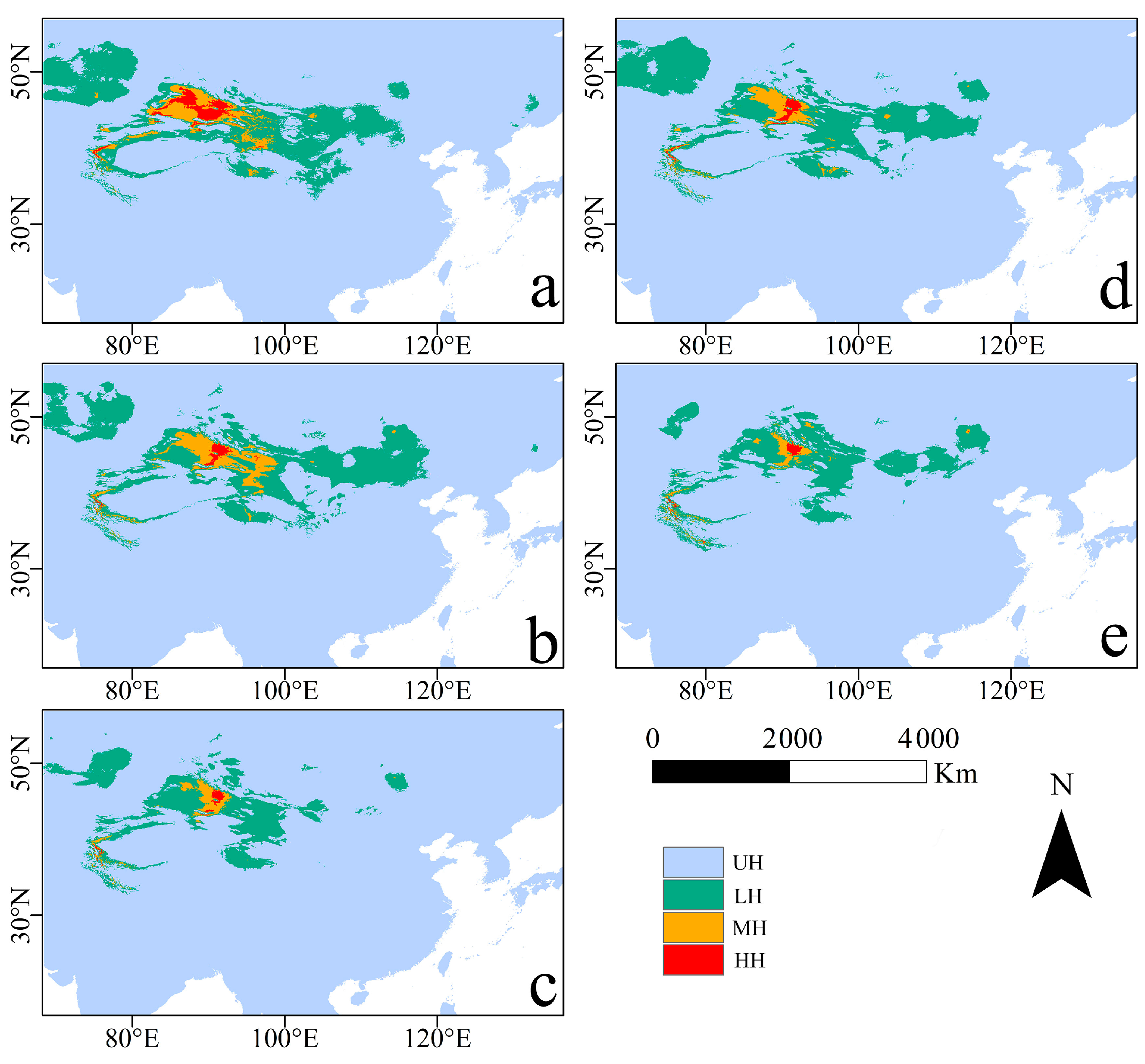
3.2. Potential Geographic Distribution and Suitable Habitat Area of R. nanum

Under the RCP2.6 and RCP6.0 scenarios, R. nanum’s potential geographic distribution of suitable habitats over the three periods (current, 2050s and 2070s) modeled by MaxEnt was visualized by ArcGIS (Figure 2). The distribution maps showed that, under current climate conditions, the range of MH was bounded at 81.7–97.3° E, 39.4–48.6° N, and the range of HH was bounded at 82.4–93.4° E, 42.5–47.9° N.
The areas of MH and HH were 361,875.0 ± 3.61 km2 and 156,284.7 ± 0.99 km2 in the current climate conditions, respectively (Figure 3). The area of suitable habitats (LH, MH, and HH) under the RCP6.0 scenario was smaller than that under the RCP2.6 scenario, in both the 2050s and the 2070s. Under the RCP2.6 scenario and the RCP6.0 scenario, the area of MH in the 2070s would be 225,972.2 ± 3.12 km2 and 123,750 ± 2.36 km2, respectively, while that of the HH in the 2070s would be 48,194.4 ± 0.54 km2 and 27,309.0 ± 0.35 km2. For MH, the area that was reduced the most was 2070RCP60 (65.80%), followed by 2050RCP60 (62.15%) and 2070RCP26 (37.56%) (Figure 2 and Table S2). For HH, the area that was reduced the most was 2070RCP60 (128,975.7 km2, 82.53%), followed by 2050RCP60 (128,368.1 km2, 82.14%), 2050RCP26 (110,920.1 km2, 70.97%), and 2070RCP26 (108,090.3 km2, 69.16%) (Figure 3 and Table S2).

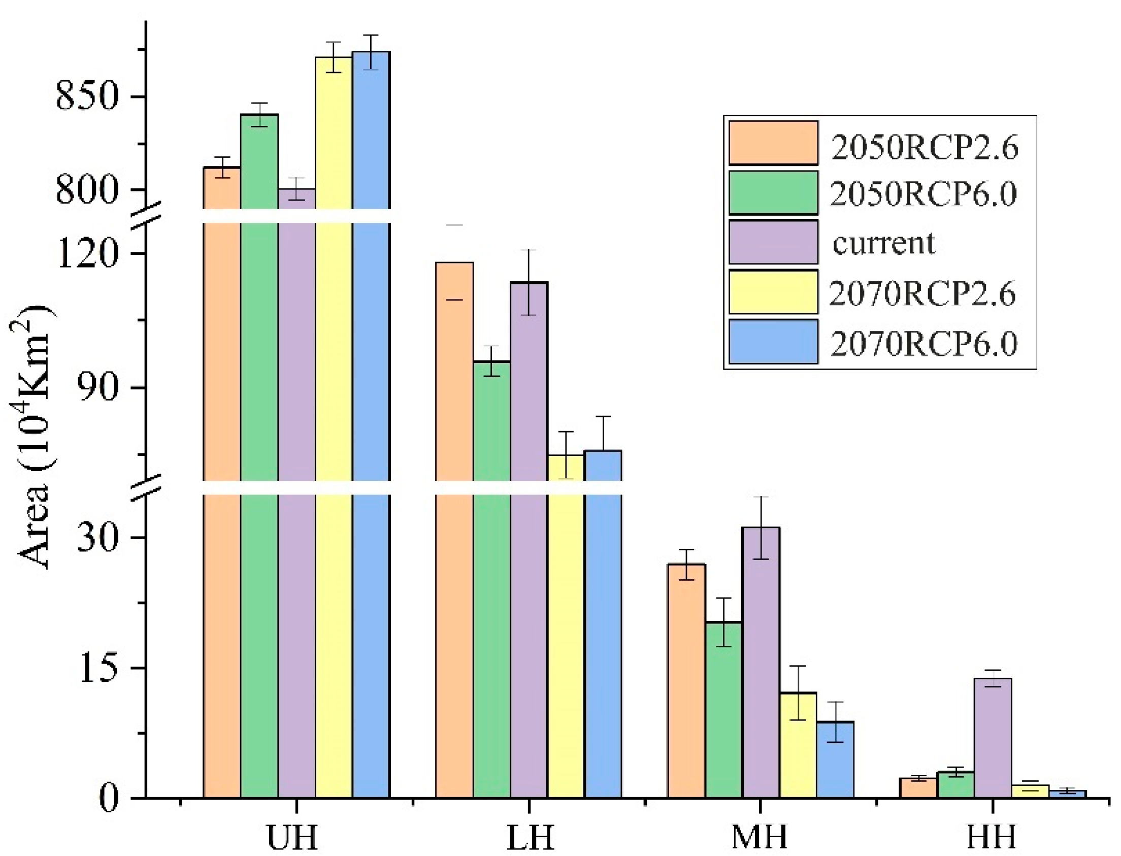
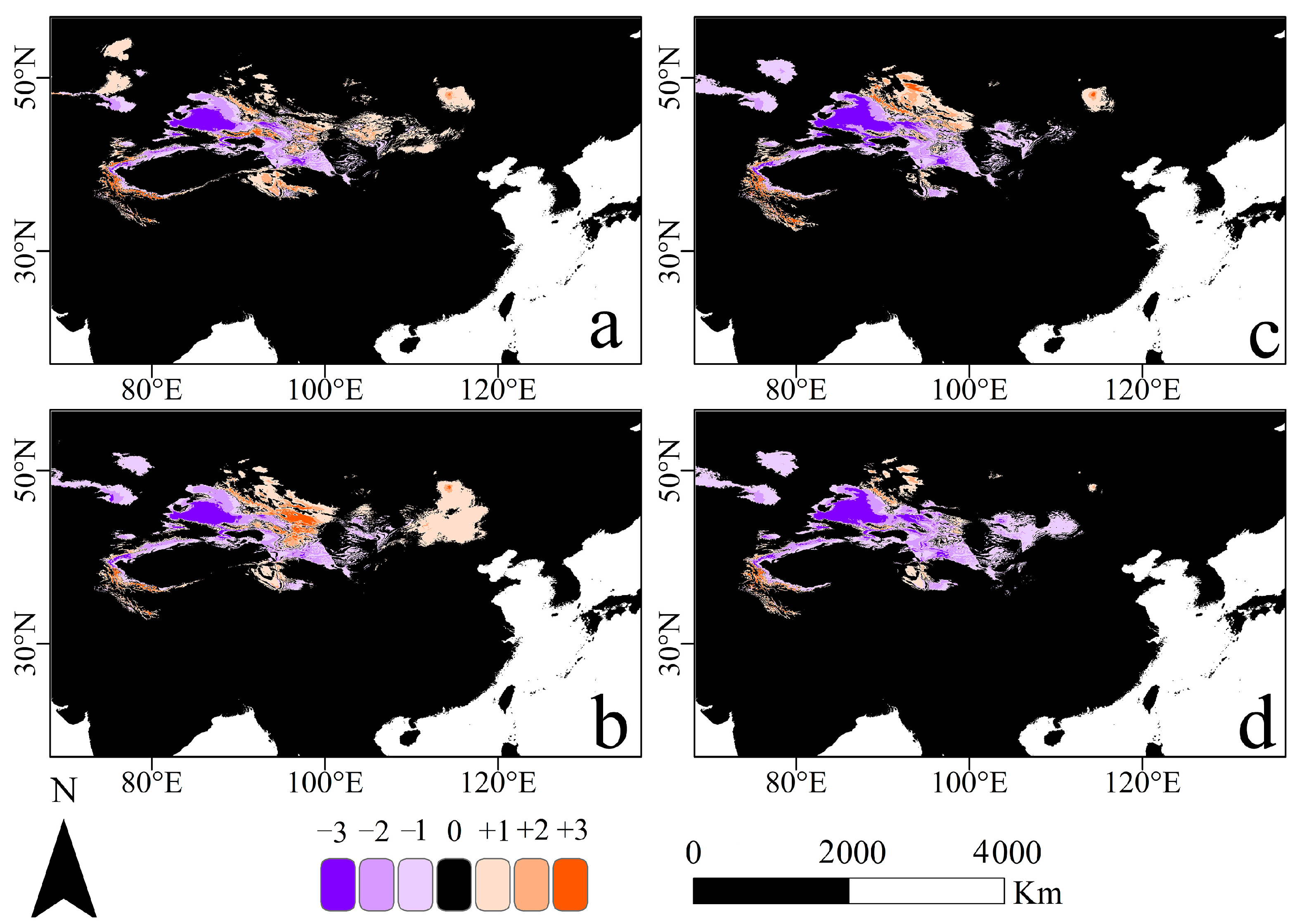
3.3. Changes of Potential Suitable Habitats in the Future Distribution Pattern

Environment variables have a significant influence on the distribution of R. nanum. The increase and decrease maps (Figure 4) described the changes in their potential suitable habitats for three periods (current, 2050s, and 2070s). The predicted maps showed that, under the RCP2.6 scenario, the habitat suitability drastically decreased in the ranges of 81.6–89.6° E, 43.6–46.8° N (Figure 4a) and 82.0–90.3° E, 43.8–46.5° N (Figure 4b) in 2070–current and 2050–current period, respectively; under the RCP6.0 scenario, the drastically decreased area of habitat suitability in 2070–current period was at 81.9–91.9° E, 42.1–48.3° N (Figure 4c), while that of 2050–current period was at 81.9–90.6° E, 43.6–48.1° N (Figure 4d). Under the RCP2.6 and RCP6.0 scenarios, the changes in habitat suitability were varied by different degrees: a larger proportion of suitability change was found between adjacent levels (e.g., MH and HH), and a smaller proportion of change was found between further apart habitat levels (e.g., LH and HH). The change range of habitat suitability at −1 and +1 was 51.84–59.31% and 65.64–76.91%, while that of −3 and +3 was 14.82–18.63% and 4.55–7.37%, respectively (Figure 4 and Table S3). Among all conditions of the 2050s and the 2070s, compared with the current distribution pattern, RCP6.0 led to a larger change in the ratio of −1 than RCP2.6, and led to a smaller change in +1 (Table S3).

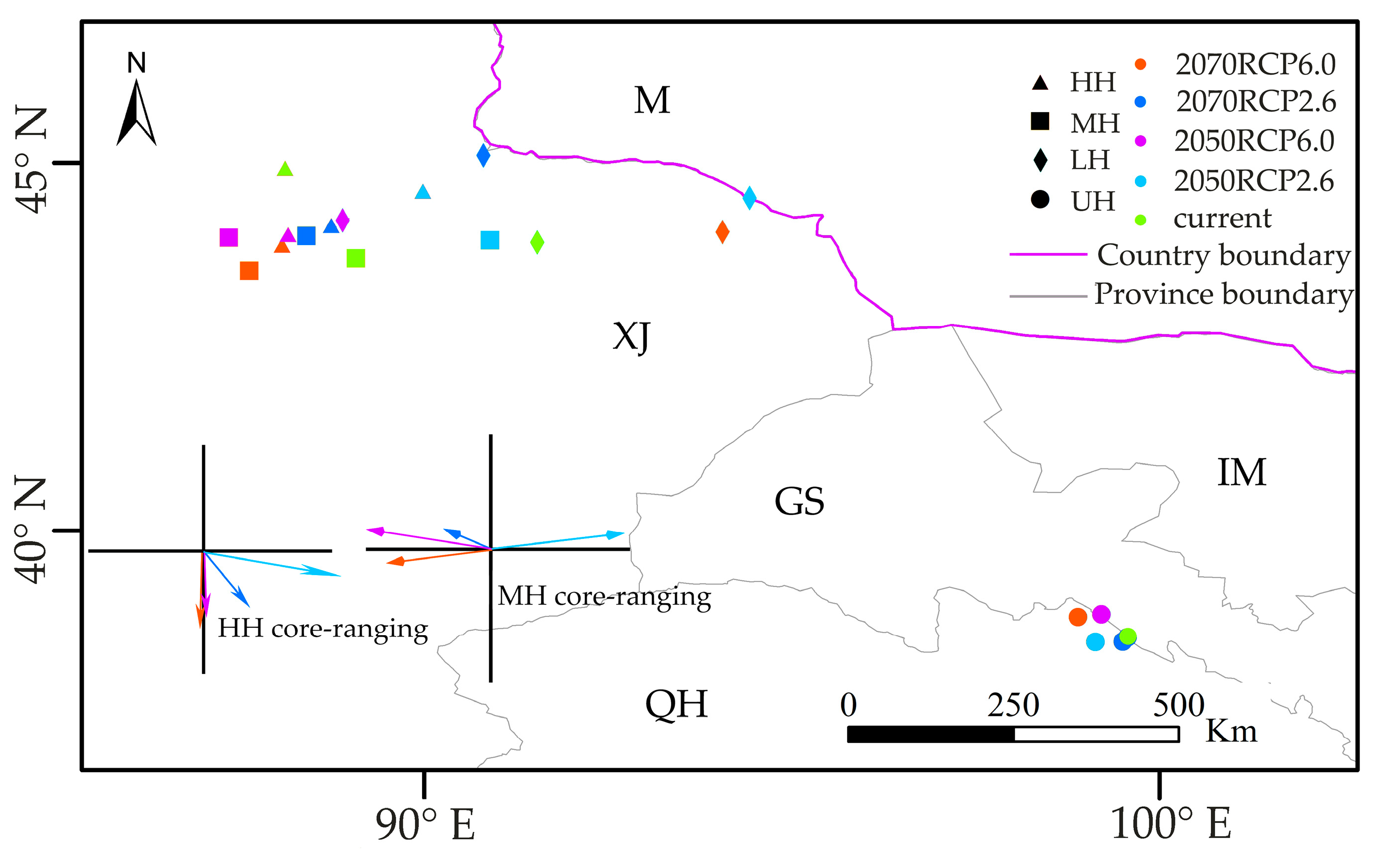
3.4. Range Shifts of Suitable Habitat Cores under Two Climate Scenarios

Under the RCP2.6 and RCP6.0 scenarios, all cores of R. nanum’s UH were located in the area of 98.7–99.6° E, 38.3–39.0° N, the border of Gansu (GS) and Qinghai (QH), and did not have significant changes for three periods (current, 2050s, and 2070s) (Figure 5). However, the cores of LH, MH, and HH in future periods (i.e., 2050s and 2070s) had significant changes under RCP2.6 and RCP6.0, compared with their current distribution. Notably, under the RCP2.6 and the RCP6.0 scenarios, all cores of LH, MH, and HH in the 2050s and the 2070s were located in Xinjiang (XJ), China (Figure 5). Compared to the habitat range of MH in the current period, in the west–east direction, the MH cores of 2050RCP60, 2070RCP26, and 2070RCP60 shifted toward the west, while the MH core of 2050RCP26 moved east; in the north–south direction, except for 2070RCP60, the MH range of 2050RCP60, 2070RCP26, and 2050RCP26 shifted toward the north (Figure 5). The shift distances of MH cores between the current distribution and that of 2070RCP60, 2070RCP26, 2050RCP60, and 2050RCP26 were 118.68 km, 63.52 km, 142.73 km, and 148.49 km, respectively. Compared to the core of HH in the current distribution, all cores of HH shifted toward the south under the RCP2.6 and the RCP6.0 future scenarios (Figure 5). Compared with the range of HH in the current distribution, the cores of HH shifted by 100.18 km and 115.65 km in 2050RCP60 and 2070RCP60, respectively.

4. Discussion

4.1. Effects of Climate Change on Suitable Habitat Range

Our simulation of the potential distribution of R. nanum in the current period, the 2050s, and the 2070s had an accurate performance (AUC > 0.9), and the results indicated that R. nanum’s distribution was largely influenced by three precipitation factors (i.e., bio14, bio16, and bio19) and one temperature factor (bio1). For flora species, precipitation affects soil moisture and infiltration [15] and plays a key role in determining the distribution of plants. Moreover, under the growing pressure of changing environments, an increase in temperature [34] has resulted in a reduction in precipitation in Himachal Pradesh, and has impacted the productivity of agricultural crops [63]. In this study, we compared the range changes of the potential suitable habitat of three periods (i.e., current, 2050s, and 2070s) under two climate scenarios (i.e., RCP2.6 and RCP6.0) to quantify the impacts of temperature increase on the potential distribution of R. nanum. Compared to the current distribution, almost every suitable habitat (LH, MH, and HH) under RCP2.6 and RCP6.0 scenarios would decrease by different degrees in the future except for LH (increase of 2.58%) and MH (increase of 2.32%) under the 2050RCP2.6 scenario (Figure 3 and Table S2). We believe that, under the 2050RCP2.6 scenario, the unbalanced changes of suitable habitats (e.g., for MH, the degraded area from HH could not offset the newly added suitable habitats from UH) may be responsible for the increase of LH and MH. The comparison of the potential distribution maps of the 2050s and the 2070s (Figure 4 and Table S2) revealed that, compared to the RCP2.6 scenario, RCP6.0 led to a greater reduction in the area of suitable habitats (LH, MH, and HH), which was contrary to previous studies [27] and our former hypotheses. The ecosystems of arid and semi-arid regions are too sensitive to global warming [64], and we believe that this may be the cause of this opposite result.
As the optimal habitat of R. nanum, the range of HH was predicted to shift south in the future, as compared to its current range. This result is contrary to the moving direction of the other species in previous studies [27,65]. We inferred that species in arid and semi-arid lands may have different survival strategies [36] when facing global warming, as compared to species in other ecosystems [26], and this may have caused the opposite range shifts. Murray et al. [66] suggested that species with a limited distribution always have a narrow ecological tolerance, and that even slight climate changes may affect their distribution patterns. In addition to the poleward shift, the cores of HH also shifted to higher altitudes with complex terrain (Figure S2), which was consistent with our original hypothesis. Previous studies have also indicated that species would shift poleward and upward to adapt to climate changes [67,68,69]. However, the poleward migration is essentially the same strategy as the high-elevation migration. For species with little elevation change in their typical habitats, range shifts north would provide an environment similar to their previous habitat in terms of temperature, and species could also shift to a colder environment by increasing living elevation by a small range [65]. Notably, unlike the simple horizon or elevation shift shown on maps, species’ range shifts in nature are typically a combination of two migration strategies [67].
With a continued increase in greenhouse gas emissions [48], the higher-emission scenario (RCP6.0) had higher rates of temperature increases than those found in the lower-emission scenario (RCP2.6). Until the end of this century, MH and HH had further range shifts in RCP6.0 than in RCP2.6. One possible reason was that, as an arid and semi-arid species [36], R. nanum is highly sensitive to climate changes (e.g., temperature and precipitation). Notably, the geometric comparison of the suitable habitat range maps of the three periods under the two climate scenarios indicated that the HH range of 2050RCP26, 2050RCP60, 2070RCP26, and 2070RCP60 were all included in the HH area in the present day (Figure 2). In addition, the global temperature and mountain ranges largely led to the range shifts of plant species [68]. Therefore, combined with the range of suitable habitats and their range shifts, we assumed that the irregular shrinkage of their suitable habitats may be the main reason behind the range shifts in the future. For insight into the essentials of species range shifts, quantifying and evaluating the importance and contribution of the irregular shrinkage of their habitats should be a focus in future studies.

4.2. Conservation of Species in Ecologically Fragile Areas

The complex terrains of the high mountains in Asia, such as the Kunlun Mountains, the Altai Mountains, the Qilian Mountains, and the Tianshan–Pamir–Hindu Kush–Karakoram mountain ranges, have created a large region with relatively stable arid and semi-arid environments [70]. Previous studies have also proven that the valleys and the rivers of the Hengduan Mountains have provided refuge for plants to survive and evolve in the Last Interglacial and the Last Glacial Maximum [71]. For the habitat suitability of R. nanum, the drastically increased range was commonly bounded by 74.1–81.4° E and 36.0–37.6° N while the drastically decreased range was commonly bounded by 81.6–89.6° E and 43.6–46.8° N (Figure 4). We speculate that the mountain regions of Central Asia provide a relatively stable habitat for R. nanum to survive, and previous studies have provided some consistent clues [27,70,71]. Under two climate scenarios of the 2050s and the 2070s, the decreased range of habitat suitability coincides with the major distribution range (MH and HH) of R. nanum under current climate conditions (Figure 2a and Figure 4). We support the belief that the ecosystems in arid and semi-arid regions are relatively fragile and sensitive to environmental changes [36], and believe that temperature and corresponding precipitation changes [34,35] may be the dominant factors causing the decrease in R. nanum’s habitat suitability in Central Asia. The growing pressure of potential evaporation caused by the increasing global warming will accelerate the decrease in soil moisture [72], which may trigger severe droughts [36] with increasing frequency in arid and semi-arid regions. The severe drought stress could lead to low richness patterns of plant species [73], which would likely offer less opportunities [74] for the adaption and distribution of species in this region.
The variations (e.g., seasonality changes) in environmental factors (i.e., temperature and precipitation [41]) have an obvious effect on flora plants in arid and semi-arid areas. Compared with the herbaceous species distributed in this region, the living strategies (e.g., deeper root systems [36]) of woody species play an important role in ensuring survival. However, they also limit the speciation during their life history and may reduce their potential distribution range [75]. In terms of the decrease in the habitat suitability and irregular shrinkage of habitat range of R. nanum, compared to species with similar habitats, we cannot state with certainty whether this is an individualistic response [41] by the species to climate change. When it comes to conservation, for R. nanum and other plants with medicinal properties [48], we hold the opinion that appropriate human intervention is necessary. Since the extinction of species due to severe climate change is most likely to occur in sensitive and fragile ecosystems (e.g., the Taklamakan Desert [36]), it is recommended that protection areas [76] are set up with suitable habitats for target species in order to prevent excessive digging [77] and illegal trade [48]. Additionally, to ensure the management and protection of agricultural crops of economic value, regular collection of field germplasm resources and corresponding artificial cultures are also necessary and deserve special attention.

4.3. Dominant Environmental Factors and Limitations in Predicting Species-Distribution Ranges

Our study succeeded in predicting the geographic distribution of species living in arid and semi-arid regions. Objectively speaking, however, our results had several limitations. Firstly, MaxEnt’s niche simulation of the target species is based on the premise that the species would be extensively present in the sites where their environmental conditions (i.e., temperature and precipitation) have maximum similarity to the sites of known occurrence data [59,62,78]. Some geographic barriers (e.g., monsoons, mountains, and rivers) that affect the distribution ranges of species are typically ignored [20]. Secondly, we only obtained a few occurrence data in this study, and the prediction did not consider more relative environment factors (i.e., soil category, light, terrain). For more accurate predictions, future studies should consider as many relevant factors (e.g., abiotic and biotic factors) as possible and integrate them with more adaptable algorithms [53]. Thirdly, we predicted the potential distribution of R. nanum using MaxEnt alone. However, previous studies have shown that crosslinked models have had a higher prediction accuracy compared to a single model [68]. In addition, as an important complement and confirmation of our work, studies of the Last Glacial Maximum [45] and the Mid-Holocene will further refine species’ response theory to climate change.

5. Conclusions

In this study, with the help of ArcGIS and the MaxEnt model, we successfully predicted R. nanum’s potential distribution and evaluated suitable habitats in the current period, the 2050s, and the 2070s under the RCP2.6 and RCP6.0 scenarios based upon the relevant environmental factors (i.e., temperature and precipitation). In contrast to the simulation of other species with abundant occurrence data, we categorized the selected occurrence data into the test layer and training layer manually, and realized MaxEnt’s effective utilization of our small sample size. Our results suggest that the potential distribution habitat of R. nanum’s range was 81.7–97.3° E and 39.4–48.6° N in the current period. The key environmental factors that affected the distribution of R. nanum were bio1 and bio16. Under the two climate scenarios, the areas of suitable habitats (i.e., LH, MH, and HH) had different degrees of decreasing in both the 2050s and the 2070s, and RCP6.0 led to larger habitat range reductions than those found with RCP2.6. Moreover, the suitable habitats for R. nanum will shift toward the south with different distances in the future. In particular, we found that the irregular shrinkage of suitable habitats may be an ignored reason that led to the movement of habitat cores. To prevent the illegal digging and trade of agricultural crops with economic value, it is feasible to establish protection areas and management standards. We believe our study can provide a vital reference for the habitat simulation of species with a small sample size, and may provide supports for species conservation in arid and semi-arid regions.

Supplementary Materials

The following supporting information can be downloaded at: https://www.mdpi.com/article/10.3390/agriculture12050610/s1, Figure S1: The curves of the MaxEnt model (a) and bio-climate factors (b) and Jackknife test results (c); Figure S2: The terrain remote sensing image (300 km) of high suitable habitat cores; Table S1: Contribution of environmental variables used in MaxEnt; Table S2: Area changes of suitable habitats in different climate scenarios; Table S3: The area (104 km2) and ratio (%) of habitat suitability change at different period interval situations.

Author Contributions

W.X. designed the study, collected occurrence data, and wrote the main body of the manuscript; W.X., S.Z. and T.Y. drew the map, tables, and figures; J.J. and J.C. acquired the funding and revised the manuscript and figures. All authors have read and agreed to the published version of the manuscript.

Funding

This study was financially supported by the Key Research and Development Program of Shaanxi Province (2021NY-006), Natural Science Foundation of China (31601987), China Agriculture Research System (CARS-34), Doctoral Fund of Henan Polytechnic University (B2019-4), and Deployment Program of the Chinese Academy of Sciences (KJZD-EW-TZ-G10).

Acknowledgments

We thank the national and international organizations that provided data and associated software for this work. The authors are indebted to Yixian Chen, Hanqi Liu, and Kai Jin for their kind help with ArcGIS operation and data processing. Junru Wang assisted in confirming species’ Latin names. During the two and a half years of fieldwork, Weiwei Ren and numerous anonymous and kind individuals helped collect the species’ field occurrence data. Moreover, we would like to thank Shuo Wang for her suggestions on the color selection of the full-text Figures. Importantly, the spiritual support of Runzhi Mao was the indispensable base for the completion of this work. We also thank the anonymous reviewers who made many important suggestions for improving the paper and others who contributed to the improvement of this manuscript.

Conflicts of Interest

The authors declare no conflict of interest.

References

  1. Xie, Z. Ecogeographical distribution of the species from Rheum.L (polygonaceae) in China. In Proceedings of the Third National Symposium on the Conservation and Sustainable Use of Biological Diversity, Kunming, China, 11−13 December 1998. [Google Scholar]
  2. Zhu, R. The Survey of Rhubarb Resources in Guyuan Country and Its Geographical Distribution. Master’s Thesis, Lanzhou University, Lanzhou, China, 2011. [Google Scholar]
  3. Zhe, W. A Study on the Pharmacophylogeny of the Rheum L. in China. Ph.D. Thesis, Chinese Academy of Medical Scienses & Peking Union Medical College, Beijing, China, 2011. [Google Scholar]
  4. Shang, X.-F.; Zhao, Z.-M.; Li, J.-C.; Yang, G.-Z.; Liu, Y.-Q.; Dai, L.-X.; Zhang, Z.-J.; Yang, Z.-G.; Miao, X.-L.; Yang, C.-J.; et al. Insecticidal and antifungal activities of Rheum palmatum L. anthraquinones and structurally related compounds. Ind. Crops Prod. 2019, 137, 508–520. [Google Scholar] [CrossRef]
  5. Yuan, S.; Jian, T.; Li, W.; Huang, Y. Extraction process optimization and activity assays of antioxidative substances from Rheum officinale. J. Food Meas. Charact. 2019, 14, 176–184. [Google Scholar] [CrossRef]
  6. Zhang, Q.; Hu, F.; Guo, F.; Zhou, Q.; Xiang, H.; Shang, D. Emodin attenuates adenosine triphosphate-induced pancreatic ductal cell injury in vitro via the inhibition of the P2X7/NLRP3 signaling pathway. Oncol. Rep. 2019, 42, 1589–1597. [Google Scholar] [CrossRef] [PubMed]
  7. Kalkan, S.; Otag, M.R.; Engin, M.S. Physicochemical and bioactive properties of edible methylcellulose films containing Rheum ribes L. extract. Food Chem. 2020, 307, 125524. [Google Scholar] [CrossRef]
  8. Qin, T.; Wu, L.; Hua, Q.; Song, Z.; Pan, Y.; Liu, T. Prediction of the mechanisms of action of Shenkang in chronic kidney disease: A network pharmacology study and experimental validation. J. Ethnopharmacol. 2020, 246, 112128. [Google Scholar] [CrossRef]
  9. Li, A.; Gao, Z.; Mao, Z. (Eds.) Flora of China; Science Press: Beijing, China, 1998; Volume 25. [Google Scholar]
  10. Kwon, H.C.; Kim, T.Y.; Lee, C.M.; Lee, K.S.; Lee, K.K. Active compound chrysophanol of Cassia tora seeds suppresses heat-induced lipogenesis via inactivation of JNK/p38 MAPK signaling in human sebocytes. Lipids Health 2019, 18, 135. [Google Scholar] [CrossRef] [Green Version]
  11. Dai, G.; Ding, K.; Cao, Q.; Xu, T.; He, F.; Liu, S.; Ju, W. Emodin suppresses growth and invasion of colorectal cancer cells by inhibiting VEGFR2. Eur. J. Pharmacol. 2019, 859, 172525. [Google Scholar] [CrossRef]
  12. Sun, J.; Luo, J.-W.; Yao, W.-J.; Luo, X.-T.; Wei, Y.-H. Effect of emodin on gut microbiota of rats with acute kidney failure. China J. Chin. Mater. Med. 2019, 44, 758–764. [Google Scholar] [CrossRef]
  13. Guo, Y.; Li, X.; Zhao, Z.; Wei, H.; Gao, B.; Gu, W. Prediction of the potential geographic distribution of the ectomycorrhizal mushroom Tricholoma matsutake under multiple climate change scenarios. Sci. Rep. 2017, 7, 46221. [Google Scholar] [CrossRef] [Green Version]
  14. Phillips, S.J.; Anderson, R.P.; Schapire, R.E. Maximum entropy modeling of species geographic distributions. Ecol. Model. 2006, 190, 231–259. [Google Scholar] [CrossRef] [Green Version]
  15. Abolmaali, S.M.-R.; Tarkesh, M.; Bashari, H. MaxEnt modeling for predicting suitable habitats and identifying the effects of climate change on a threatened species, Daphne mucronata, in central Iran. Ecol. Inform. 2018, 43, 116–123. [Google Scholar] [CrossRef]
  16. Papes, M.; Gaubert, P. Modelling ecological niches from low numbers of occurrences: Assessment of the conservation status of poorly known viverrids (Mammalia, Carnivora) across two continents. Divers. Distrib. 2007, 13, 890–902. [Google Scholar] [CrossRef]
  17. Tang, J.; Cheng, Y.; Luo, L.; Zhang, L.; Jiang, X. Maxent-based prediction of overwintering areas of Loxostege sticticalis in China under different climate changes scenarios. Acta Ecol. Sin. 2017, 37, 4852–4863. [Google Scholar] [CrossRef]
  18. Araujo, M.B.; Pearson, R.G.; Thuiller, W.; Erhard, M. Validation of species-climate impact models under climate change. Glob. Chang. Biol. 2005, 11, 1504–1513. [Google Scholar] [CrossRef] [Green Version]
  19. Peterson, A.T. Uses and Requirements of Ecological Niche Models and Related Distributional Models. Biodivers. Inform. 2006, 3, 59–72. [Google Scholar] [CrossRef] [Green Version]
  20. Phillips, S.J.; Dudik, M. Modeling of species distributions with Maxent: New extensions and a comprehensive evaluation. Ecography 2008, 31, 161–175. [Google Scholar] [CrossRef]
  21. Guisan, A.; Zimmermann, N.E. Predictive habitat distribution models in ecology. Ecol. Model. 2000, 135, 147–186. [Google Scholar] [CrossRef]
  22. Elith, J.; Graham, C.H.; Anderson, R.P.; Dudik, M.; Ferrier, S.; Guisan, A.; Hijmans, R.J.; Huettmann, F.; Leathwick, J.R.; Lehmann, A.; et al. Novel methods improve prediction of species’ distributions from occurrence data. Ecography 2006, 29, 129–151. [Google Scholar] [CrossRef] [Green Version]
  23. Garcia, K.; Lasco, R.; Ines, A.; Lyon, B.; Pulhin, F. Predicting geographic distribution and habitat suitability due to climate change of selected threatened forest tree species in the. Philippines. Appl. Geogr. 2013, 44, 12–22. [Google Scholar] [CrossRef]
  24. Illoldi-Rangel, P.; Sanchez-Cordero, V.; Peterson, A.T. Predicting distributions of Mexican mammals using ecological niche modeling. J. Mammal. 2004, 85, 658–662. [Google Scholar] [CrossRef] [Green Version]
  25. Remya, K.; Ramachandran, A.; Jayakumar, S. Predicting the current and future suitable habitat distribution of Myristica dactyloides Gaertn. using MaxEnt model in the Eastern Ghats, India. Ecol. Eng. 2015, 82, 184–188. [Google Scholar] [CrossRef]
  26. Zhang, K.; Yao, L.; Meng, J.; Tao, J. Maxent modeling for predicting the potential geographical distribution of two peony species under climate change. Sci. Total Environ. 2018, 634, 1326–1334. [Google Scholar] [CrossRef] [PubMed]
  27. Ma, B.; Sun, J. Predicting the distribution of Stipa purpurea across the Tibetan Plateau via the MaxEnt model. BMC Ecol. 2018, 18, 10. [Google Scholar] [CrossRef] [PubMed] [Green Version]
  28. Ciss, M.; Biteye, B.; Fall, A.G.; Fall, M.; Gahn, M.C.B.; Leroux, L.; Apolloni, A. Ecological niche modelling to estimate the distribution of Culicoides, potential vectors of bluetongue virus in Senegal. BMC Ecol. 2019, 19, 45. [Google Scholar] [CrossRef] [Green Version]
  29. Guo, Y.L.; Li, X.; Zhao, Z.F.; Nawaz, Z. Predicting the impacts of climate change, soils and vegetation types on the geographic distribution of Polyporus umbellatus in China. Sci. Total Environ. 2019, 648, 1–11. [Google Scholar] [CrossRef] [PubMed]
  30. Qin, A.; Liu, B.; Guo, Q.; Bussmann, R.W.; Ma, F.; Jian, Z.; Xu, G.; Pei, S. Maxent modeling for predicting impacts of climate change on the potential distribution of Thuja sutchuenensis Franch., an extremely endangered conifer from southwestern China. Glob. Ecol. Conserv. 2017, 10, 139–146. [Google Scholar] [CrossRef]
  31. Root, T.L.; Price, J.T.; Hall, K.R.; Schneider, S.H.; Rosenzweig, C.; Pounds, J.A. Fingerprints of global warming on wild animals and plants. Nature 2003, 421, 57–60. [Google Scholar] [CrossRef] [PubMed]
  32. Xu, W.; Jin, J.; Cheng, J. Predicting the Potential Geographic Distribution and Habitat Suitability of Two Economic Forest Trees on the Loess Plateau, China. Forests 2021, 12, 747. [Google Scholar] [CrossRef]
  33. Xu, X.; Zhang, H.; Yue, J.; Xie, T.; Xu, Y.; Tian, Y. Predicting Shifts in the Suitable Climatic Distribution of Walnut (Juglans regia L.) in China: Maximum Entropy Model Paves the Way to Forest Management. Forests 2018, 9, 103. [Google Scholar] [CrossRef] [Green Version]
  34. Bracegirdle, T.J.; Krinner, G.; Tonelli, M.; Haumann, F.A.; Naughten, K.A.; Rackow, T.; Roach, L.A.; Wainer, I. Twenty first century changes in Antarctic and Southern Ocean surface climate in CMIP6. Atmos. Sci. Lett. 2020, 14, e984. [Google Scholar] [CrossRef]
  35. Kellermann, V.; van Heerwaarden, B. Terrestrial insects and climate change: Adaptive responses in key traits. Physiol. Entomol. 2019, 44, 99–115. [Google Scholar] [CrossRef] [Green Version]
  36. Sun, Y.; Sun, Y.; Yao, S.R.; Akram, M.A.; Hu, W.G.; Dong, L.W.; Li, H.L.; Wei, M.H.; Gong, H.Y.; Xie, S.B.; et al. Impact of climate change on plant species richness across drylands in China: From past to present and into the future. Ecol. Indic. 2021, 132, 108288. [Google Scholar] [CrossRef]
  37. Sun, J.; Qin, X.; Yang, J. The response of vegetation dynamics of the different alpine grassland types to temperature and precipitation on the Tibetan Plateau. Environ. Monit. Assess. 2016, 188, 20. [Google Scholar] [CrossRef] [PubMed] [Green Version]
  38. Hughes, L. Biological consequences of global warming: Is the signal already apparent? Trends Ecol. Evol. 2000, 15, 56–61. [Google Scholar] [CrossRef]
  39. Piao, S.L.; Liu, Q.; Chen, A.P.; Janssens, I.A.; Fu, Y.S.; Dai, J.H.; Liu, L.L.; Lian, X.; Shen, M.G.; Zhu, X.L. Plant phenology and global climate change: Current progresses and challenges. Glob. Chang. Biol. 2019, 25, 1922–1940. [Google Scholar] [CrossRef]
  40. Iannella, M.; De Simone, W.; D’Alessandro, P.; Biondi, M. Climate change favours connectivity between virus-bearing pest and rice cultivations in sub-Saharan Africa, depressing local economies. Peerj 2021, 9, e12387. [Google Scholar] [CrossRef]
  41. Alexander, J.M.; Chalmandrier, L.; Lenoir, J.; Burgess, T.I.; Essl, F.; Haider, S.; Kueffer, C.; McDougall, K.; Milbau, A.; Nunez, M.A.; et al. Lags in the response of mountain plant communities to climate change. Glob. Chang. Biol. 2018, 24, 563–579. [Google Scholar] [CrossRef]
  42. Pepin, N.; Bradley, R.S.; Diaz, H.F.; Baraer, M.; Caceres, E.B.; Forsythe, N.; Fowler, H.; Greenwood, G.; Hashmi, M.Z.; Liu, X.D.; et al. Elevation-dependent warming in mountain regions of the world. Nat. Clim. Chang. 2015, 5, 424–430. [Google Scholar] [CrossRef] [Green Version]
  43. Wang, L.; Wang, W.J.; Wu, Z.F.; Du, H.B.; Zong, S.W.; Ma, S. Potential Distribution Shifts of Plant Species under Climate Change in Changbai Mountains, China. Forests 2019, 10, 498. [Google Scholar] [CrossRef] [Green Version]
  44. Shankhwar, R.; Bhandari, M.S.; Meena, R.K.; Shekhar, C.; Pandey, V.V.; Saxena, J.; Kant, R.; Barthwal, S.; Naithani, H.B.; Pandey, S.; et al. Potential eco-distribution mapping of Myrica esculenta in northwestern Himalayas. Ecol. Eng. 2019, 128, 98–111. [Google Scholar] [CrossRef]
  45. Wang, S.; Xu, X.; Shrestha, N.; Zimmermann, N.E.; Wang, Z. Response of spatial vegetation distribution in China to climate changes since the Last Glacial Maximum (LGM). PLoS ONE 2017, 12, e0175742. [Google Scholar] [CrossRef] [PubMed] [Green Version]
  46. Wu, Y.M.; Shen, X.L.; Tong, L.; Lei, F.W.; Zhang, Z.X. Impact of Past and Future Climate Change on the Potential Distribution of an Endangered Montane Shrub Lonicera oblata and Its Conservation Implications. Forests 2021, 12, 125. [Google Scholar] [CrossRef]
  47. Tian, B.J.; Dong, X.Y. The Double-ITCZ Bias in CMIP3, CMIP5, and CMIP6 Models Based on Annual Mean Precipitation. Geophys. Res. Lett. 2020, 47, 11. [Google Scholar] [CrossRef] [Green Version]
  48. Shrestha, B.; Tsiftsis, S.; Chapagain, D.J.; Khadka, C.; Bhattarai, P.; Kayastha Shrestha, N.; Alicja Kolanowska, M.; Kindlmann, P. Suitability of Habitats in Nepal for Dactylorhiza hatagirea Now and under Predicted Future Changes in Climate. Plants 2021, 10, 467. [Google Scholar] [CrossRef]
  49. van Vuuren, D.P.; Stehfest, E.; den Elzen, M.G.J.; Kram, T.; van Vliet, J.; Deetman, S.; Isaac, M.; Goldewijk, K.K.; Hof, A.; Beltran, A.M.; et al. RCP2.6: Exploring the possibility to keep global mean temperature increase below 2 degrees C. Clim. Chang. 2011, 109, 95–116. [Google Scholar] [CrossRef]
  50. O’Neill, B.C.; Tebaldi, C.; van Vuuren, D.P.; Eyring, V.; Friedlingstein, P.; Hurtt, G.; Knutti, R.; Kriegler, E.; Lamarque, J.F.; Lowe, J.; et al. The Scenario Model Intercomparison Project (ScenarioMIP) for CMIP6. Geosci. Model Dev. 2016, 9, 3461–3482. [Google Scholar] [CrossRef] [Green Version]
  51. Rana, S.K.; Rana, H.K.; Ghimire, S.K.; Shrestha, K.K.; Ranjitkar, S. Predicting the impact of climate change on the distribution of two threatened Himalayan medicinal plants of Liliaceae in Nepal. J. Mt. Sci. 2017, 14, 558–570. [Google Scholar] [CrossRef]
  52. Xin, X.G.; Zhang, L.; Zhang, J.; Wu, T.W.; Fang, Y.J. Climate Change Projections over East Asia with BCC_CSM1.1 Climate Model under RCP Scenarios. J. Meteorol. Soc. Jpn. 2013, 91, 413–429. [Google Scholar] [CrossRef] [Green Version]
  53. Breiner, F.T.; Guisan, A.; Bergamini, A.; Nobis, M.P. Overcoming limitations of modelling rare species by using ensembles of small models. Methods Ecol. Evol. 2015, 6, 1210–1218. [Google Scholar] [CrossRef]
  54. Hu, X.; Wu, F.; Guo, W.; Liu, N. Identification of Potential Cultivation Region fie Santalum album in China by the MaxEnt Ecologic Niche Model. Sci. Silvae Sin. 2014, 50, 27–33. [Google Scholar] [CrossRef]
  55. Fu, G.Q.; Xu, X.Y.; Ma, J.P.; Xu, M.S.; Jiang, L.; Ding, A.Q. Responses of Haloxylon ammodendron potential geographical distribution to the hydrothermal conditions under MaxEnt model. Pratacult. Sci. 2016, 33, 2173–2179. [Google Scholar] [CrossRef]
  56. Elith, J.; Phillips, S.J.; Hastie, T.; Dudik, M.; Chee, Y.E.; Yates, C.J. A statistical explanation of MaxEnt for ecologists. Divers. Distrib. 2011, 17, 43–57. [Google Scholar] [CrossRef]
  57. Lv, W.; Li, Z.; Wu, X.; Ni, W.; Qv, W. Maximum Entropy Niche-Based Modeling (Maxent) of Potential Geographical Distributions of Lobesia Botrana (Lepidoptera: Tortricidae) in China; Springer: Berlin/Heidelberg, Germany, 2012. [Google Scholar]
  58. Hernandez, P.A.; Graham, C.H.; Master, L.L.; Albert, D.L. The effect of sample size and species characteristics on performance of different species distribution modeling methods. Ecography 2006, 29, 773–785. [Google Scholar] [CrossRef]
  59. Guisan, A.; Graham, C.H.; Elith, J.; Huettmann, F.; Distri, N.S. Sensitivity of predictive species distribution models to change in grain size. Divers. Distrib. 2007, 13, 332–340. [Google Scholar] [CrossRef]
  60. Graham, M.H. Confronting multicollinearity in ecological multiple regression. Ecology 2003, 84, 2809–2815. [Google Scholar] [CrossRef] [Green Version]
  61. Vaughan, I.P.; Ormerod, S.J. The Continuing Challenges of Testing Species Distribution Models. J. Appl. Ecol. 2005, 42, 720–730. [Google Scholar] [CrossRef]
  62. Xu, W.; Sun, H.; Jin, J.; Cheng, J. Predicting the Potential Distribution of Apple Canker Pathogen (Valsa mali) in China under Climate Change. Forests 2020, 11, 1126. [Google Scholar] [CrossRef]
  63. Rana, R.S.; Singh, M.; Pathania, R.; Upadhyay, S.K.; Kalia, V. Impact of changes in climatic conditions on temperate fruit production of Himachal Pradesh. Mausam 2017, 68, 655–662. [Google Scholar] [CrossRef]
  64. Yan, X.; Zhang, Q.; Yan, X.; Wang, S.; Ren, X.; Zhao, F. An Overview of Distribution Characteristics and Formation Mechanisms in Global Arid Areas. Adv. Earth Sci. 2019, 34, 826–841. [Google Scholar] [CrossRef]
  65. Ribeiro, M.M.; Roque, N.; Ribeiro, S.; Gavinhos, C.; Castanheira, I.; Quinta-Nova, L.; Albuquerque, T.; Gerassis, S. Bioclimatic modeling in the Last Glacial Maximum, Mid-Holocene and facing future climatic changes in the strawberry tree (Arbutus unedo L.). PLoS ONE 2019, 14, 15. [Google Scholar] [CrossRef] [Green Version]
  66. Murray, K.A.; Rosauer, D.; McCallum, H.; Skerratt, L.F. Integrating species traits with extrinsic threats: Closing the gap between predicting and preventing species declines. Proc. Biol. Sci. 2011, 278, 1515–1523. [Google Scholar] [CrossRef] [Green Version]
  67. Lenoir, J.; Gegout, J.C.; Marquet, P.A.; de Ruffray, P.; Brisse, H. A Significant Upward Shift in Plant Species Optimum Elevation During the 20th Century. Science 2008, 320, 1768–1771. [Google Scholar] [CrossRef] [PubMed]
  68. Yu, F.Y.; Wang, T.J.; Groen, T.A.; Skidmore, A.K.; Yang, X.F.; Ma, K.P.; Wu, Z.F. Climate and land use changes will degrade the distribution of Rhododendrons in China. Sci. Total Environ. 2019, 659, 515–528. [Google Scholar] [CrossRef] [PubMed]
  69. Chen, I.C.; Hill, J.K.; Ohlemuller, R.; Roy, D.B.; Thomas, C.D. Rapid Range Shifts of Species Associated with High Levels of Climate Warming. Science 2011, 333, 1024–1026. [Google Scholar] [CrossRef] [PubMed]
  70. Li, J.; McCarthy, T.M.; Wang, H.; Weckworth, B.V.; Schaller, G.B.; Mishra, C.; Lu, Z.; Beissinger, S.R. Climate refugia of snow leopards in High Asia. Biol. Conserv. 2016, 203, 188–196. [Google Scholar] [CrossRef]
  71. Hu, Z.-j.; Zhang, Y.-l.; Yu, H.-b. Simulation of Stipa purpurea disttibution pattern on Tibetan Plateau based on MaxEnt model. Chin. J. Appl. Ecol. 2015, 26, 505–511. [Google Scholar] [CrossRef]
  72. Sato, T.; Kimura, F.; Kitoh, A. Projection of global warming onto regional precipitation over Mongolia using a regional climate model. J. Hydrol. 2007, 333, 144–154. [Google Scholar] [CrossRef]
  73. Brown, S.C.; Wigley, T.M.L.; Otto-Bliesner, B.L.; Rahbek, C.; Fordham, D.A. Persistent Quaternary climate refugia are hospices for biodiversity in the Anthropocene. Nat. Clim. Change 2020, 10, 244–248. [Google Scholar] [CrossRef]
  74. Ron, R.; Fragman-Sapir, O.; Kadmon, R. The role of species pools in determining species diversity in spatially heterogeneous communities. J. Ecol. 2018, 106, 1023–1032. [Google Scholar] [CrossRef]
  75. Albuquerque, F.S.; Olalla-Tarraga, M.A.; Montoya, D.; Rodriguez, M.A. Environmental determinants of woody and herb plant species richness patterns in Great Britain. Ecoscience 2011, 18, 394–401. [Google Scholar] [CrossRef]
  76. Kaky, E.; Gilbert, F. Using species distribution models to assess the importance of Egypt’s protected areas for the conservation of medicinal plants. J. Arid. Environ. 2016, 135, 140–146. [Google Scholar] [CrossRef] [Green Version]
  77. Bhattarai, P.; Pandey, B.; Gautam, R.K.; Chhetri, R. Ecology and Conservation Status of Threatened Orchid Dactylorhiza hatagirea (D. Don) Soo in Manaslu Conservation Area, Central Nepal. Am. J. Plant Sci. 2014, 5, 3483–3491. [Google Scholar] [CrossRef] [Green Version]
  78. Guisan, A.; Thuiller, W. Predicting species distribution: Offering more than simple habitat models. Ecol. Lett. 2005, 8, 993–1009. [Google Scholar] [CrossRef] [PubMed]
Figure 1. Occurrence data of Rheum nanum in China.
Agriculture 12 00610 g001
Figure 2. Potential suitable habitat maps of the current period, 2050s, and 2070s: (a) current; (b) 2050RCP2.6; (c) 2050RCP6.0; (d) 2070RCP2.6; (e) 2070RCP6.0. UH, LH, MH, and HH represent unsuitable habitat, low suitable habitat, middle suitable habitat, and high suitable habitat, respectively.
Agriculture 12 00610 g002
Figure 3. The area of potential suitable habitats over three periods (current, 2050s, and 2070s) under RCP2.6 and RCP6.0 scenarios. UH, LH, MH, and HH represent unsuitable habitat, low suitable habitat, middle suitable habitat, and high suitable habitat, respectively.
Agriculture 12 00610 g003
Figure 4. The increase and decrease maps of suitable habitats area: (a,b) RCP2.6 scenario; (c,d) RCP6.0 scenario; (a,c) 2070–current; (b,d) 2050–current. Zero represents no change of suitability, negative numbers represent a decrease in habitat suitability, and positive numbers represent an increase in habitat suitability. The degree of habitat suitability changes increases from −1 to −3 and +1 to +3.
Agriculture 12 00610 g004
Figure 5. Range shifts of four habitats under RCP2.6 and RCP6.0 scenarios. Lines with color show the direction and distance of core change from current (start of line) to specific time (end of arrow) in MH and HH, and the color of the line depicts the specific time. UH: unsuitable habitat; LH: low suitable habitat; MH: middle suitable habitat; HH: high suitable habitat; M: Mongolia; IM: Inner Mongolia; XJ: Xinjiang; GS: Gansu; QH: Qinghai.
Agriculture 12 00610 g005
Table 1. Environmental variables used for MaxEnt modeling.
CodeBioclimatic DataUnitContribution (%)Importance (%)
bio1Annual mean temperature°C13.9 ± 0.854.1 ± 2.7
bio9Mean temperature of driest quarter°C7.4 ± 0.63.1 ± 0.6
bio14Precipitation of driest monthmm9.7 ± 1.80.1 ± 0.1
bio15Precipitation seasonality 6.2 ± 1.19.3 ± 2.1
bio16Precipitation of wettest quartermm55.9 ± 2.120.0 ± 5.3
bio19Precipitation of coldest quartermm6.9 ± 2.213.4 ± 2.6
Publisher’s Note: MDPI stays neutral with regard to jurisdictional claims in published maps and institutional affiliations.

