Article

Improving Winter Wheat Yield Forecasting Based on Multi-Source Data and Machine Learning

1
Key Laboratory of Land Surface Pattern and Simulation, Institute of Geographic Sciences and Natural Resources Research, CAS, Beijing 100101, China
2
College of Resources and Environment, University of Chinese Academy of Sciences, Beijing 100049, China
3
Natural Resources Institute Finland (Luke), 00790 Helsinki, Finland
4
Barley Research Department, Field Crops Research Institute, Agricultural Research Center, Giza 583121, Egypt
5
Medicinal and Aromatic Plants Department, Horticulture Research Institute, Agricultural Research Center, Giza 583121, Egypt
*
Author to whom correspondence should be addressed.
Agriculture 2022, 12(5), 571; https://doi.org/10.3390/agriculture12050571
Submission received: 21 March 2022 / Revised: 15 April 2022 / Accepted: 16 April 2022 / Published: 19 April 2022
(This article belongs to the Special Issue Modeling the Adaptations of Agricultural Production to Climate Change)

Abstract

:
To meet the challenges of climate change, population growth, and an increasing food demand, an accurate, timely and dynamic yield estimation of regional and global crop yield is critical to food trade and policy-making. In this study, a machine learning method (Random Forest, RF) was used to estimate winter wheat yield in China from 2014 to 2018 by integrating satellite data, climate data, and geographic information. The results show that the yield estimation accuracy of RF is higher than that of the multiple linear regression method. The yield estimation accuracy can be significantly improved by using climate data and geographic information. According to the model results, the estimation accuracy of winter wheat yield increases dramatically and then flattens out over months; it approached the maximum in March, with R2 and RMSE reaching 0.87 and 488.59 kg/ha, respectively; this model can achieve a better yield forecasting at a large scale two months in advance.

1. Introduction

As the world’s largest producer and consumer of wheat [1], China faces great challenges of food security. Winter wheat production, one of the most important summer grain production of China [2], stagnated in 56% of China from 1961 to 2008 [3]. Therefore, a timely and an accurate winter wheat yield forecasting in China is of great importance for food trade and policymakers. Recently, there has been increasing research on winter wheat yield estimation where the yield prediction models are based on the physiological and the ecological processes of crops. These have been developed constantly, such as WOFOST [4], DSSAT [5], APSIM [6], STICS [7], and MONICA [8]. Such models mostly simulate daily crop development, growth, and yield formation as well as climate variables that are used as the main inputs to describe environmental conditions during the period of crop growth. However, the growth state of crops is not only affected by abiotic factors (growth environment) but also by biological factors (such as plant diseases) [9,10,11]. Therefore, using climate data alone may not be sufficient to estimate yield. Meanwhile, due to the high spatial heterogeneity of crop varieties, farmer management policies, and environments, there is significant uncertainty in the practical application of the model on a large scale [12,13].
Satellite remote sensing can continuously monitor crop growth across various spectral bands and provide useful additional information for crop yield estimations [14,15,16]. In the past decades, remote sensing monitoring technology has been successfully applied to crop yield estimations [17,18]. Such research was mostly about the empirical relationship between vegetation indexes (VIs), which is based on visible light and near infrared (e.g., NDVI data, are important in the models of crop yield estimation [19,20,21,22], radiation data EVI, GCVI) [23,24,25,26], and observed yield [27]. EVI, which is sensitive to a higher canopy leaf area index and less affected by the atmospheric aerosol, is most commonly used in crop yield estimation. However, VIs are based on greenness and not sensitive to the physiological changes of vegetation caused by meteorological factors such as temperature, vapor pressure, and absorbed radiation. In recent years, extensive studies have shown [28,29,30,31] that sun-induced chlorophyll fluorescence (SIF) can directly reflect the respiration of crops, respond timely and accurately to environmental stress, and it is directly related to biomass [32,33,34,35]. Currently some studies use SIF directly to estimate crop yield and to obtain better results at the field scale than the vegetation index [29,36,37,38]. It has been shown that the yield estimation accuracy of crop models based on climate data and on satellite data is generally better than that of the models based on data alone [39,40,41]. Water-supply-related variables (such as precipitation), temperature-related variables (such as maximum temperature), and water-demand-related variables (such as potential evapotranspiration), among all climate are also important variables for crop growth simulation [42]. Recognizing that various satellite products have common overlapping and complementary information is conducive to yield estimation [43]. However, better combining satellite data with other environmental factors in crop yield estimation needs to be further studied [44]. It is also unclear how multi-source climate data (i.e., climate and satellite data) promote the formation of the final yield estimation models and how their contributions to the models vary with the growing season. Furthermore, more and more approaches based on machine learning (ML) or deep learning are applied to agricultural applications, such as crop type classification [45,46], disease prediction [47], crop growth monitoring [48], and yield estimation [49,50,51,52]. Frausto-Solis [53] estimated the yield of many kinds of crops based on data of daily minimum and maximum temperature, and precipitation by using the decision tree (DT), while Jeong [54] used climate data to estimate the yields of wheat and corn and other crops in the world and some regions based on RF. At present, the research on the estimation of winter wheat yield in China based on RF are mostly concentrated in the North China Plain, such as Anhui Province, Henan Province, and so on [54,55,56].
To avoid the randomness of an individual model, this paper used multiple linear regression (MLR), a most common method for forecasting, and random forest (RF), a typical machine learning method, to build a crop yield estimation model in which the crop growth environment, agricultural policies, and spatial heterogeneity of yield are considered. This model combines the spatial information data, the climate data, and the satellite data. This paper aims to understand the relationship between different input elements and crop yield and to compare the effects of different input data combinations and time series data of different growth periods on the model’s performance. Besides, this paper intends to unravel and to quantify the contributions of climate and satellite data on growing seasons to the crop yield estimation. This study mainly used EVI and SIF to find out whether satellite data can improve climate-based yield estimation methods on a large scale and also to explore whether SIF still maintains the advantage of the sensitive capture of photosynthetic activity of crops on a large scale [57,58].

2. Materials and Methods

2.1. Study Area

As the target area in this study, the winter wheat planting areas in China (Figure 1) are mainly in the North China Plain and also include the winter wheat planting area in ten provinces—Inner Mongolia, Shandong, Hubei, Chongqing, Sichuan, Guizhou, Yunnan, Shaanxi, Gansu, and Qinghai—and two autonomous regions: Ningxia and Xinjiang. It is thus clear that the study area is widely distributed and the proportion of planting areas in other provinces are relatively small. Winter wheat in China is generally sown at the end of September or at the beginning of October, and it is harvested by the middle of June of the following year [59]. Generally, irrigation and fertilization are available in these areas. In this study, January to June is defined as the major growth period of winter wheat on which the analysis and the modeling are focused in view of the effect of cold and frost injury on crops in January [60].

2.2. Data and Preprocessing

2.2.1. Dataset

The study uses data on crop yield, planting area, satellite data, climate data, and spatial information (Table 1). The multi-source data collected in the study have various temporal and spatial resolutions. Therefore, firstly the raster data were resampled to a spatial resolution of 1 km and the climate and satellite data are unified into monthly interval. Then, monthly climate and satellite are aggregated at prefecture-level by using the crop map generated.
Crop yield and planting area: the winter wheat yield of prefecture-level cities from 2014 to 2018 (unit: kg/ha) was collected from local agricultural statistical yearbooks. Based on the previous work, winter wheat planting distribution of China at 1 km resolution from 2000 to 2015 are identified [61] (https://doi.org/10.6084/m9.figshare.8313530 (accessed on 21 August 2019)). The main planting areas of crops remain almost unchanged in a short period, therefore in this study the data of 2014 is used to represent the winter wheat planting distribution in China from 2014 to 2018.
Satellite data: satellite data includes EVI (MOD13C2 V6) (https://search.earthdata.nasa.gov (accessed on 1 February 2000)) and SIF reanalysis datasets (GOSIF) of OCO-2 satellite (http://data.globalecology.unh.edu (accessed on 27 November 2019)). Compared with the normalized vegetation index (NDVI), EVI is closely related to biomass and crop yield [62], and it can better represent the leaf and the chlorophyll content of crop canopy; GOSIF is a reanalysis dataset based on SIF data derived from OCO-2, MODIS data, and climate data. Compared with SIF data with coarse resolution and calculated directly from OCO-2, GOSIF has a better spatio-temporal resolution (0.05°, 8 days), continuous global coverage, and longer records.
Climate data: a total of 10 climate variables are collected from CRU_TS 4.04 (Climatic Research Unit Timeseries 4.04) series and CMFD (The China Meteorological Forcing Dataset) series (Table 1). The CRU_TS series is based on the record analysis of more than 4000 independent weather stations and it is gridded at a resolution of 0.5 × 0.5°, including monthly precipitation, daily maximum and minimum temperatures, cloud cover, and other variables covering the terrestrial region of the earth from 1901 to 2020. The CMFD dataset, with a spatial resolution of 0.1 × 0.1°, mainly includes precipitation per 3 h, surface radiation, wind speed, air specific humidity, and other variables covering 1979 to 2018.
Geographical basic data: the crops growth status and growth environment have spatial heterogeneity. Studies have indicated that crop yields in neighboring counties are usually similar in a certain year. The spatial autocorrelation can be explained by coding geographical coordinates (lat, lon) in feature space [62,63]. In this study, all data, including EVI, SIF, climate variables, and geographical coding, are covered by the raster data of winter wheat distribution and they were collected to prefecture-level cities with an average value.

2.2.2. Data Preprocessing

Selecting input variables was indispensable before machine learning and linear regression, which can not only reduce the input dimension, i.e., integrating expert knowledge to select the most appropriate input but also quantify the correlation between different potential independent variables and dependent variables to help to explain the results of machine learning algorithms. Based on previous studies on the relation between climate and crop yield [19,20,21,22], ten climate variables were selected for the study. To facilitate variable selection and interpretation, the best variable combinations of yield estimation were chosen without wasting information. Firstly, the 10 climate variables were divided into four groups according to prior knowledge: (1) water-supply-related, including precipitation (pre), wet day frequency (wet), and air specific humidity (shum); (2) temperature-related, including near-surface average temperature (tmp), near-surface temperature minimum (tmn), and near-surface temperature maximum (tmx); (3) water-demand-related, including potential evapotranspiration (pet) and vapor pressure (vap); and (4) radiation-related, including surface downward shortwave radiation (srad) and surface downward longwave radiation (lrad). The correlation analysis was carried out based on the mean value of the variables of the growing season (January–June) to eliminate the influence of the seasonal cycle. This study selected appropriate dependent variable inputs from the climate variables based on the following criteria: 1) selecting the variables which have the maximum absolute correlation with the yield in each group; and 2) selecting the variables whose value of correlation with the previously selected climate variables in the same group is not greater than 0.5.

2.3. Research Methods

2.3.1. Multiple Linear Regression

Multiple linear regression (MLR) is one of the most widely used methods of crop yield estimation, and it is easy to use. Based on the principle of Ordinary Least Square (OLS) and the stepwise regression method, the independent variables were selected with significant effects and they constructed the optimal regression model for winter wheat yield estimation by using the climate, satellite, and space information data. The yield estimation model is calculated by Equation (1)
Y = a 1 x 1 + a 2 x 2 + a 3 x 3 a n x n + β + ε
where Y represents the winter wheat yield of prefecture-level cities; x1…xn represent different independent variable factors used to predict Y; a1…an represent partial regression coefficient; β is a random variable and a constant term; and ε represents random error. The criterion for the stepwise regression model to pass the significance test is that the equation of linear relation model passes the F test and all the coefficients of the equation passes the t test.

2.3.2. Random Forest

Random Forest (RF) is an integrated learning technology, which classifies or regresses by combining a group of CART decision trees. Due to the introduction of randomness, RF is not prone to over-fitting, and it has good learning stability [56]. In this paper, the scikit-learn, an ML library of Python, is used to develop the RF model, which includes three steps: (1) normalizing all the selected variables and yield and randomly dividing the whole data set into training data with 70% and test data with 30% [64,65]; (2) for the training data set only, optimizing the key parameters of each model based on the highest R2 and the lowest RMSE by ten-fold cross-verification; and (3) conducting the “leave one year out” experiment from 2014 to 2018, and R2 and RMSE are used to evaluate the performance and generalization of the model. Considering the climate data, satellite data, and spatial information, this study counts the yield data of 187 out of 385 prefecture-level cities in China from 2014 to 2018.

2.4. Experiment Design

Two groups of experiments were designed (Figure 2) to answer the research questions raised in this paper. The purpose of the first group of experiments was to explore the effect of different input combinations on crop yield estimation models and to compare the potential of SIF in crop yield estimation. There are 11 data input combinations for the experiment, namely: (1) only SIF; (2) only EVI; (3) only climate; (4) SIF combined with spatial information; (5) EVI combined with spatial information; (6) climate combined with spatial information; (7) SIF combined with climate; (8) EVI combined with climate; (9) SIF combined with climate and spatial information; (10) EVI combined with climate and spatial information; and (11) SIF combined with EVI, climate, and spatial information. To assess the practicality of these models, based on the most suitable selected input, we recursively performed hindcasting for each year from 2014 to 2018 to evaluate whether the models can be promoted in different years; for example, the data for 2014–2017 was collected as training data to predict winter wheat yield in 2018. Certainly, future data cannot be used to predict current data. However, more verification samples can be provided for these hypotheses to increase the understanding of the model’s performance. The RMSE (root mean square error) and R2 (determination coefficient) between the predicted yield and the actual yield of winter wheat were calculated to verify the accuracy of the model.
The second group of experiments explored the effect of time series data on yield estimation models and the contribution of climate data and satellite data to crop yield prediction at different growth stages. In this experiment, the location information was not added since by default the spatial information of crops remained unchanged in this study in the short term. In the experiments, the climate and the satellite data were added and compared the change of R2 and RMSE based on two methods of modeling to evaluate the change of performance of winter wheat estimation models. During the growing season (January–June), the input data of all months were used to predict winter wheat yield. The experiments were based on the three input combinations (namely climate, satellite, as well as climate and satellite). According to the experiment results, the added value of climate or satellite data to the estimation model in any period can be determined, and through different methods and input combinations the time for the model to achieve the best performance of estimation can be tested.

3. Results

3.1. Selection of Climate Variables Combination

Figure 3 shows the correlation analysis results of 10 climate variables, which demonstrated that water-supply-related variables (shum, pre, and wet) are all positively correlated with yield, while tmx and tmp among the temperature-related variables are negatively correlated with yield. Among the water-demand-related variables, pet is negatively correlated with yield, while vap is positively correlated with yield. Among radiation-related variables, srad is negatively correlated with yield, and lrad is positively correlated with yield. To select appropriate variables from each group as the input of yield estimation, 5 out of 10 climate variables are selected according to the method in Section 2.4, namely wet, tmx, pet, srad, and vap.

3.2. The Influence of Different Input Data Combinations on the Simulation of the Model

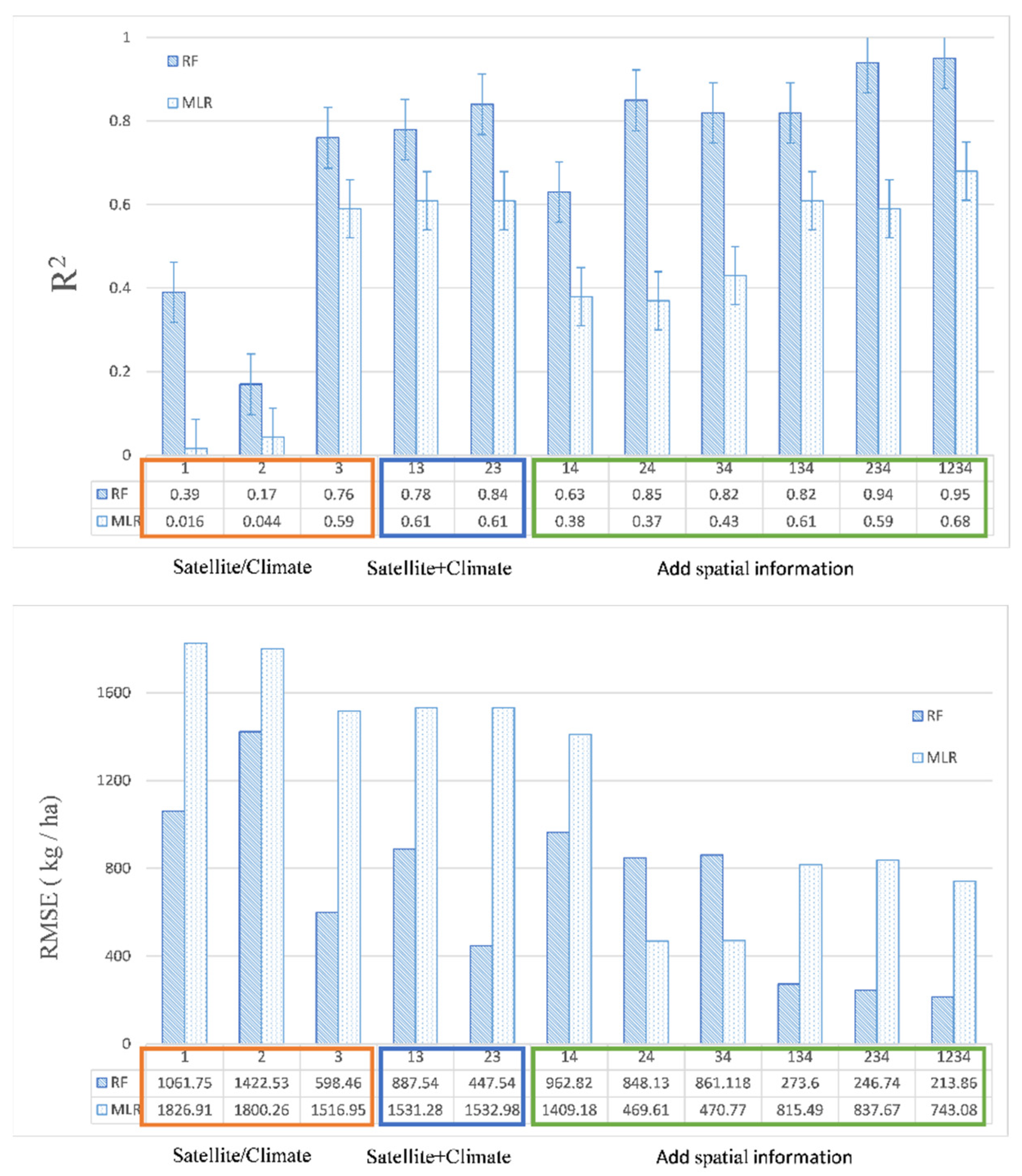
The results of the first group of experiments given in (Figure 4) that two models have the following similar characteristics with different combinations of data inputs: in the single data, the yield estimation performance of climate data is better. It may be because the climate variables can better simulate the growing environment of crops. There is an obvious spatial pattern of winter wheat yield at the prefecture scale, which indicates that the addition of spatial information is helpful to improve the prediction accuracy of the model. A better simulated result of yield is obtained by combining satellite data, climate data, and spatial information (MLR: R2~0.68; RF: R2~0.95). What is noteworthy is that on a monthly scale, compared with the addition of EVI, that of SIF does not significantly improve the yield estimation accuracy. The estimation effect of RF by combining SIF with other environmental factors is even lower than that of EVI. The result indicates that at the seasonal and the prefecture scale, SIF cannot provide much additional information that is different from EVI in crop yield estimation, and it shows no advantages of yield estimation on the small scale in the field. This may be related to the low signal-to-noise ratio, coarse resolution, and complex extraction algorithm of SIF [38]. However, the resolution of the SIF dataset used in this study (0.05°) has been improved compared with previous datasets (0.5~1°) [38]. Yet, the performance of the model remains the same, indicating that the downscale SIF dataset based on statistical methods alone cannot significantly enhance the effect of seasonal-scale crop yield estimation, which is consistent with Lindsey [66].

3.3. Comparison of Yield Estimation Performance of the Model

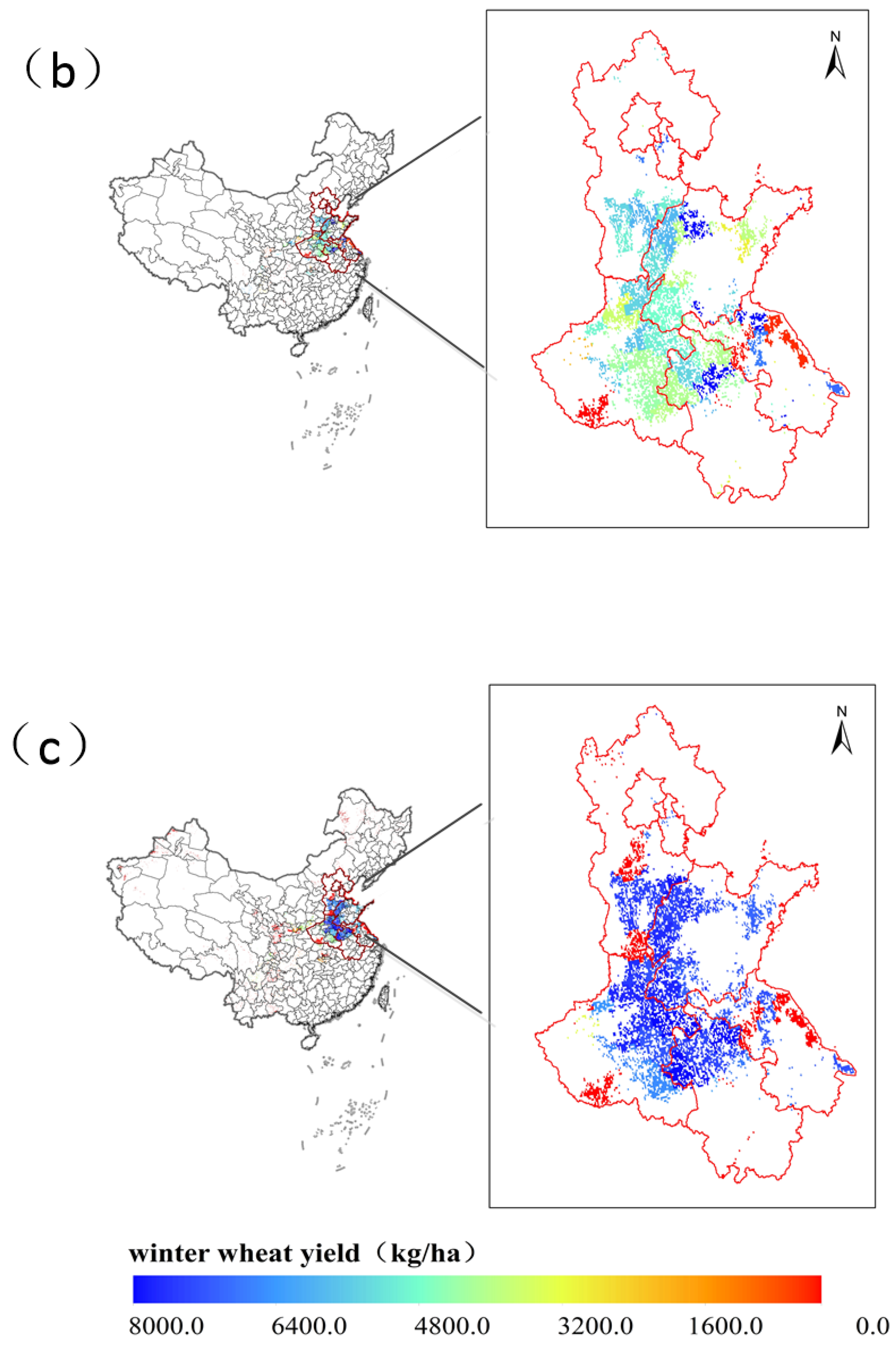
The results show that the yield estimation performance of RF is generally higher than that of MLR, which may be because the relationships between crop yield and variables are mostly nonlinear while nonlinear methods capture these relationships better than linear methods. Besides comparing the performance and generalization of the models, we conduct a “leave-one-year-out” experiment to verify the extrapolation potential of the models, which is establishing models based on all data and the crop yields in four out of five years and then separately verifying the estimated yield result of the year left. The result is shown in Table 2 in which each row represents the model performance of one year. The RMSE and R2 between the estimated and the actual yield of winter wheat are compared. The results show that R2 and RMSE are fairly stable in each year of winter wheat yield estimation at the prefecture scale, except for 2015. For example, the spatial distribution of yield prediction of 2014 based on two models (Figure 5) shows that RF can well reflect the spatial difference of winter wheat yield, especially in the North China Plain, in addition to having a high potential of yield estimation. In 2014, the errors of RF are mainly in Henan Province, while MLR generally underestimates the crop yield in high-yield areas, and the errors are concentrated in Henan, Hebei, and Shandong provinces.

3.4. The Influence of Time Series Data on the Simulation Ability of the Model

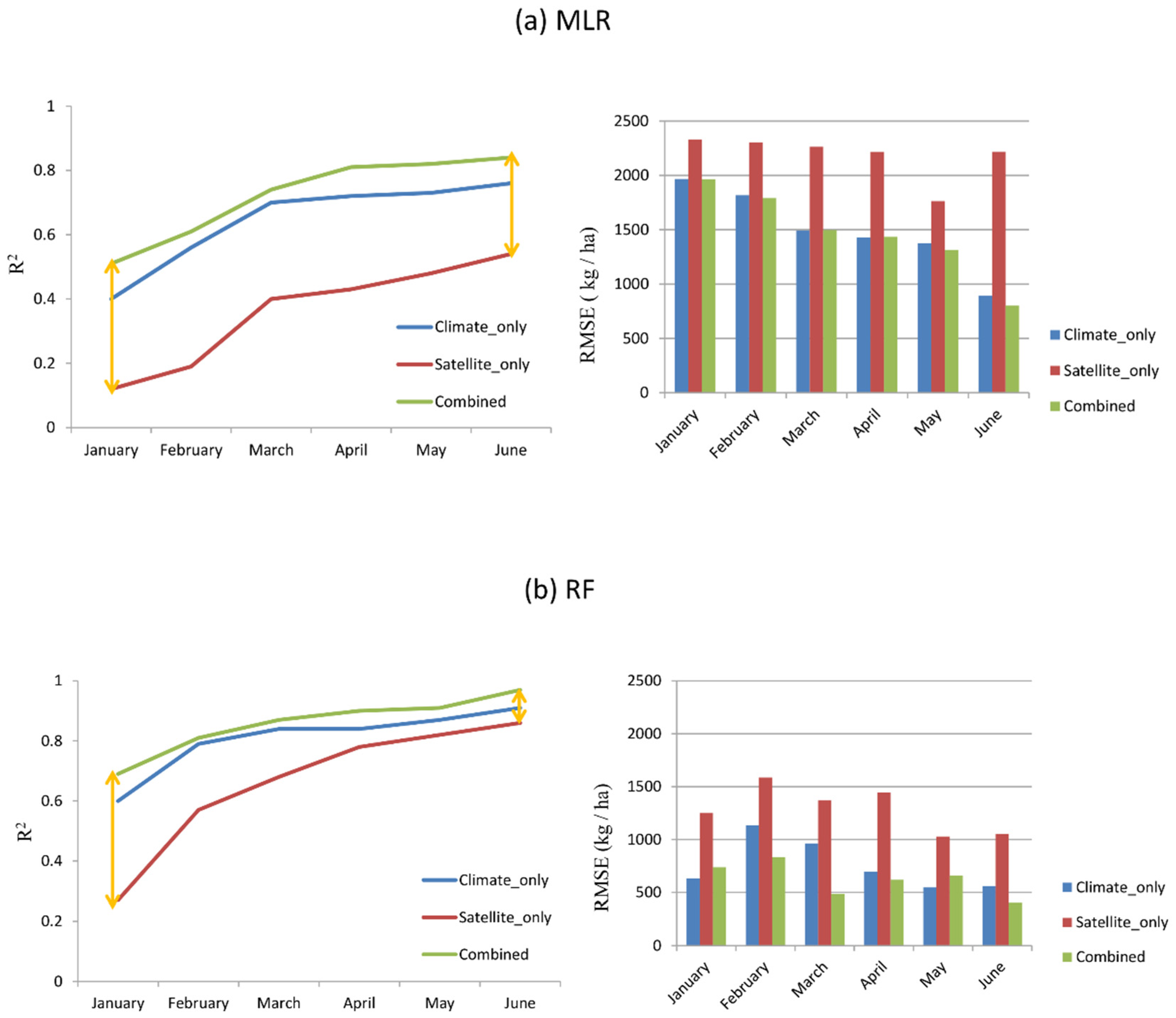
Since SIF has no advantage in large-scale yield estimation, EVI is used as an example in this experiment. The results (Figure 6) illustrate that the two models have the following similar characteristics: (1) for any particular inputs, the yield estimation accuracy of the model increases rapidly with the increase of acquired data and the growth rate slows down and gradually reaches saturation at a later stage of the growing season; (2) the combination can significantly improve the performance of the yield estimation model which can be significantly improved through combining climate data with satellite data, and climate data plays an essential role in the model. However, there are significant differences in the trajectory of model prediction performance produced by different inputs. With only satellite data as inputs, the model generally starts from very poor performance (R2~0.1–0.2), and then it improves relatively by much (R2~0.4–0.5), while with only climate data and combined data as inputs, the model starts with relatively good performance (R2~0.4–0.6) and has a small increase during the growing season. To understand more clearly the effect of multi-resource data on the model, we assume that climate and satellite data have independent and overlapping contributions to the yield estimation model. We quantify the contributions of data from different sources. For example, the independent influence of climate data on the model is the difference between the combination R2 and satellite R2. The results indicate that (Figure 7) climate data always play a vital role in the performance of the model. With the advance of the growing season, the proportion of overlapping information becomes higher, and the contribution of climate data to the model decreases gradually. The results depict that satellite data gradually absorbs climate information as time goes by. In addition, models with only climate data and only satellite data can generally achieve a high simulation performance in May, while the performance of those with multi-source data can generally get close to the maximum in March (RF) and April (MLR). Therefore, the combination of multi-source data can achieve a high estimation accuracy of the crop yield one or two months in advance.

4. Discussion

The results show the effects of different input combinations on yield estimation accuracy, and different yield estimation models have similar results. During the whole crop growing season, climate data always provide important information for crop yield estimation, which is consistent with the previous conclusions [20,21,22]. The performance of two yield estimation models with satellite data has been significantly improved, which is consistent with the view of Guan et al., who indicate that satellite data can provide for crop growth additional information different from climate data [43]. It is worth noting that the addition of SIF in the regional range does not significantly improve the yield estimation accuracy of the model in this case. Compared with EVI, SIF has no significant advantage in performance of yield estimation. It has not provided much additional information to the yield estimation model. It agrees with previous research results on whether SIF has an advantage in capturing crop growth state on the regional scale [38,66], which may be related to the coarse resolution and the complex extraction algorithm and thus more uncertainties of SIF. Random Forest can better predict crop yield. This is consistent with the literature [39], as both temperature and precipitation have a nonlinear response to yield [67,68]; and the nonlinear yield estimation model was more in line with the actual situation.
As time goes on in the growing season, the amount of the input satellite and the climate data increases, and the changes of yield estimation accuracy of different models show a similarity. In accordance with the previous conclusions [38], in the early stage of crop growth climate data play an important role in the model, the satellite gradually absorbs crop growth information, and the yield estimation accuracy of the model increases significantly, while the yield estimation accuracy reaches the maximum in the late stage of growth. It is worth noting that the time when the estimation accuracy reaches the maximum varies slightly between estimation models. While in the regression model the accuracy of yield estimation peaks only one month before harvest, RF achieves a high performance of the yield prediction two months in advance.
The winter wheat planting areas are widely distributed in China, with obvious spatial differences. The main planting areas of winter wheat are in the North China Plain, about 15,309.1 kha. Most of the previous studies have not considered the situation of Inner Mongolia, Ningxia, Xinjiang, and other regions, which accounts for approximately 27.4 percent of the total winter wheat planting area in China. This study establishes models of yield estimation at the national scale with consideration of the spatial heterogeneity of winter wheat yield by adding extra basic geographic data. The results show that adding spatial information data can improve the yield estimation accuracy of models [3] and it is helpful to establish a unified model on a large scale.
In this paper, RF and MLR are used to build yield estimation models of winter wheat in China, which avoids the randomness of single model analysis. However, due to the availability of data, the research is mainly on the prediction of crop yield at the prefecture scale. Furthermore, the spatial resolution of the satellite data used is relatively coarse, which leads to small training samples, and it limits the ability of machine learning methods [38,64,69]. The newly launched satellite provides a variety of data (such as EVI, SIF, and climate variables) and it has a higher spatiotemporal resolution (such as Landsat, Sentinel, and Fluorescence EXplorer) [70,71,72], which can provide the potential for future improvement. Besides, although the machine learning model performs well in the yield estimation in the prefecture, the process-based explanation is limited, which weakens the traceability and the interpretability of the model. How to better combine the process-based model with machine learning algorithm to realize more efficiently the extrapolation beyond the training conditions [54,69] and special migration can be investigated in the future. This is to improve the crop yield estimation of models in areas where there are not enough historical yield records, such as Africa [44]. At the same time, some key factors have not been considered in this study, such as biological factors other than those captured by satellite, namely soil characteristics [26,40], which will also help to explain more yield variability. In addition, due to the data limitation of the spatial distribution of winter wheat, the spatial distribution of winter wheat from 2014 to 2018 was represented by 2014 data in this paper, which may also lead to errors in the statistics of remote sensing data. For future research, it is suggested that the crop interannual spatial distribution information data should be generated from satellite data to reduce potential errors.

5. Conclusions

To avoid the randomness of a single model, this study conducts yield estimation of winter wheat in China at the prefecture scale based on a MLR model and a RF model combining climate data, satellite data, and spatial information. The effects of different input combinations and time-series data on the performance of the model have been discussed. The main conclusions are as follows:
(1)
By decomposing and quantifying the contribution of satellite data and climate data to the model’s performance in different growth periods, we find that satellite data can gradually capture the changes of crop growth and with accumulation of information can absorb part of the climate data. Spatial information and climate data have made a unique contribution to the yield forecasting of winter wheat in the whole growing season.
(2)
By comparing the satellite data from two sources (i.e., SIF and EVI), it was found that the downsized SIF products do not perform better than EVI on the yield forecasting at the prefecture scale in China, which may be largely owing to the low signal-to-noise ratio of SIF products and the difficulty of extraction algorithm.
(3)
By comparing the extrapolation and the spatial generalization ability of two models, RF can generally better capture the spatiotemporal heterogeneity of crop growth and thus is expected to better understand the impact of meteorology on agricultural production.
This study demonstrated a new scalable, simple, and inexpensive framework in estimating winter wheat yields over a wide range of areas based on publicly available data, which is applicable to other crops and geographical environments.

Author Contributions

S.Z. led the project and developed the framework; F.T. and S.Z. conceptualized and designed this research strategy; Y.S. carried out the field work and was responsible for data processing and manuscript writing; S.Z., R.A. and A.A. revised the manuscript. All authors have read and agreed to the published version of the manuscript.

Funding

This study was supported by the National Key Research and Development Program of China (Project No. 2016YFD0300201) and the National Science Foundation of China (Project No. 41801078).

Institutional Review Board Statement

Not applicable.

Informed Consent Statement

Not applicable.

Data Availability Statement

The data presented in this study are available on request from the authors.

Conflicts of Interest

The authors declare no conflict of interest.

References

  1. Wei, L. Spatial-temporal evolution of Wheat production in China and its influencing factors. Chin. J. Agric. Resour. Reg. Plan. 2019, 40, 49–57. [Google Scholar]
  2. Huang, J.; Tian, L.; Liang, S.; Ma, H.; Becker-Reshef, I.; Huang, Y.; Su, W.; Zhang, X.; Zhu, D.; Wu, W. Improving winter wheat yield estimation by assimilation of the leaf area index from Landsat TM and MODIS data into the WOFOST model. Agric. For. Meteorol. 2015, 204, 106–121. [Google Scholar] [CrossRef] [Green Version]
  3. Chen, Y.; Zhang, Z.; Tao, F.; Wang, P.; Wei, X. Spatio-temporal patterns of winter wheat yield potential and yield gap during the past three decades in North China. Field Crops Res. 2017, 206, 11–20. [Google Scholar] [CrossRef]
  4. Van Diepen, C.V.; Wolf, J.V.; Van Keulen, H.; Rappoldt, C. WOFOST: A simulation model of crop production. Soil Use Manag. 2010, 5, 16–24. [Google Scholar] [CrossRef]
  5. Jones, J.W.; Hoogenboom, G.; Porter, C.H.; Boote, K.J.; Batchelor, W.D.; Hunt, L.A.; Wilkens, P.W.; Singh, U.; Gijsman, A.J.; Ritchie, J.T. The DSSAT cropping system model. Eur. J. Agron. 2003, 18, 235–265. [Google Scholar] [CrossRef]
  6. Keating, B.A.; Carberry, P.S.; Hammer, G.L.; Probert, M.E.; Smith, C.J. An overview of APSIM, a model designed for farming systems simulation. Eur. J. Agron. 2003, 18, 267–288. [Google Scholar] [CrossRef] [Green Version]
  7. Brisson, N.; Gate, P.; Lorgeou, J.; Nicoullaud, B.; Justes, E. STICS: A generic model for simulating cropsand their water and nitrogen balances.II. Model validation for wheat and maize. Agronomie 2002, 22, 69–92. [Google Scholar] [CrossRef]
  8. Nendel, C.; Berg, M.; Kersebaum, K.C.; Mirschel, W.; Specka, X.; Wegehenkel, M.; Wenkel, K.O.; Wieland, R. The MONICA model: Testing predictability for crop growth, soil moisture and nitrogen dynamics. Ecol. Model. 2011, 222, 1614–1625. [Google Scholar] [CrossRef]
  9. Hatfield, J.L.; Gitelson, A.A.; Schepers, J.S.; Walthall, C.L. Application of Spectral Remote Sensing for Agronomic Decisions. Agron. J. 2008, 100, S-117–S-131. [Google Scholar] [CrossRef] [Green Version]
  10. Mahlein, A.K.; Oerke, E.C.; Steiner, U.; Dehne, H.W. Recent advances in sensing plant diseases for precision crop protection. Eur. J. Plant Pathol. 2012, 133, 197–209. [Google Scholar] [CrossRef]
  11. Lichtenthaler, H.K. Vegetation Stress: An Introduction to the Stress Concept in Plants. J. Plant Physiol. 1996, 148, 4–14. [Google Scholar] [CrossRef]
  12. Ginaldi, F.; Bajocco, S.; Bregaglio, S.; Cappelli, G. Spatializing Crop Models for Sustainable Agriculture; Springer International Publishing: Cham, Switzerland, 2019; pp. 599–619. [Google Scholar]
  13. Kamir, E.; Waldner, F.; Hochman, Z. Estimating wheat yields in Australia using climate records, satellite image time series and machine learning methods. ISPRS J. Photogramm. Remote Sens. 2020, 160, 124–135. [Google Scholar] [CrossRef]
  14. Anderson, M.C.; Hain, C.; Otkin, J.; Zhan, X.; Mo, K.; Svoboda, M.; Wardlow, B.; Pimstein, A. An Intercomparison of Drought Indicators Based on Thermal Remote Sensing and NLDAS-2 Simulations with U.S. Drought Monitor Classifications. J. Hydrometeorol. 2013, 14, 1035–1056. [Google Scholar] [CrossRef]
  15. Rodriguez, D.; Sadras, V.O.; Christensen, L.K.; Belford, R. Spatial assessment of the physiological status of wheat crops as affected by water and nitrogen supply using infrared thermal imagery. Aust. J. Agric. Res. 2005, 56, 983–993. [Google Scholar] [CrossRef]
  16. Zhang, L.; Qiao, N.; Huang, C.; Wang, S. Monitoring Drought Effects on Vegetation Productivity Using Satellite Solar-Induced Chlorophyll Fluorescence. Remote Sens. 2019, 11, 378. [Google Scholar] [CrossRef] [Green Version]
  17. Doraiswamy, P.C.; Hatfield, J.L.; Jackson, T.J.; Akhmedov, B.; Prueger, J.; Stern, A. Crop condition and yield simulations using Landsat and MODIS. Remote Sens. Environ. 2004, 92, 548–559. [Google Scholar] [CrossRef]
  18. Huang, J.; Ma, H.; Wei, S.; Zhang, X.; Wu, W. Jointly Assimilating MODIS LAI and et Products into the SWAP Model for Winter Wheat Yield Estimation. IEEE J. Sel. Top. Appl. Earth Obs. Remote Sens. 2015, 8, 4060–4071. [Google Scholar] [CrossRef]
  19. Fitzpatrick, E. Estimates of pan evaporation from mean maximum temperature and vapour pressure. J. Appl. Meteorol. 1963, 2, 780–792. [Google Scholar] [CrossRef] [Green Version]
  20. Fitzpatrick, E.A.; Nix, H.A. A model for simulating soil water regime in alternating fallow-crop systems. Agric. Meteorol. 1969, 6, 303–319. [Google Scholar] [CrossRef]
  21. Gouache, D.; Bouchon, A.-S.; Jouanneau, E.; Le Bris, X. Agrometeorological analysis and prediction of wheat yield at the departmental level in France. Agric. For. Meteorol. 2015, 209, 1–10. [Google Scholar] [CrossRef]
  22. Landau, S.; Mitchell, R.A.C.; Barnett, V.; Colls, J.J.; Craigon, J.; Payne, R.W. A parsimonious, multiple-regression model of wheat yield response to environment. Agric. For. Meteorol. 2000, 101, 151–166. [Google Scholar] [CrossRef]
  23. Hui, Q. Assessment of Net Primary Productivity (NPP) of Vegetation in North China Plain Using MODIS Remote Sensing Information; Jilin University: Changchun, China, 2004. [Google Scholar]
  24. Guo, Y.S.; Liu, Q.S.; Liu, G.H.; Huang, C. Extraction of main crop planting information based on MODIS Time series NDVI. J. Nat. Resour. 2017, 32, 1808–1818. [Google Scholar]
  25. Holzman, M.E.; Rivas, R.; Piccolo, M.C. Estimating soil moisture and the relationship with crop yield using surface temperature and vegetation index. Int. J. Appl. Earth Obs. Geoinf. 2014, 28, 181–192. [Google Scholar] [CrossRef]
  26. Potgieter, A.B.; Lawson, K.; Huete, A.R. Determining crop acreage estimates for specific winter crops using shape attributes from sequential MODIS imagery. Int. J. Appl. Earth Obs. Geoinf. 2013, 23, 254–263. [Google Scholar] [CrossRef]
  27. Cao, J.; Zhang, Z.; Tao, F.; Zhang, L.; Luo, Y.; Zhang, J.; Han, J.; Xie, J. Integrating Multi-Source Data for Rice Yield Prediction across China using Machine Learning and Deep Learning Approaches. Agric. For. Meteorol. 2021, 297, 108275. [Google Scholar] [CrossRef]
  28. Yongguang, Z. Passive Remote Sensing of Chlorophyll Fluorescence in Plants and Its Application; Zhejiang University: Zhejiang, China, 2006. [Google Scholar]
  29. Guan, K.; Berry, J.A.; Zhang, Y.; Joiner, J.; Guanter, L.; Badgley, G.; Lobell, D.B. Improving the monitoring of crop productivity using spaceborne solar-induced fluorescence. Glob. Chang. Biol. 2016, 22, 716–726. [Google Scholar] [CrossRef] [PubMed]
  30. Guanter, L.; Zhang, Y.; Jung, M.; Joiner, J.; Voigt, M.; Berry, J.A.; Frankenberg, C.; Huete, A.R.; Zarco-Tejada, P.; Lee, J.E.; et al. Global and time-resolved monitoring of crop photosynthesis with chlorophyll fluorescence. Proc. Natl. Acad. Sci. USA 2014, 111, E1327–E1333. [Google Scholar] [CrossRef] [Green Version]
  31. Zhang, Y.; Guanter, L.; Berry, J.A.; Joiner, J.; van der Tol, C.; Huete, A.; Gitelson, A.; Voigt, M.; Köhler, P. Estimation of Vegetation Photosynthetic Capacity from Space-Based Measurements of Chlorophyll Fluorescence for Terrestrial Biosphere Models. Glob. Change Biol. 2014, 20, 3727–3742. [Google Scholar] [CrossRef] [Green Version]
  32. Berry, J.; Frankenberg, C.; Wennberg, P. New Methods for Measurements of Photosynthesis from Space. 2013. Available online: https://authors.library.caltech.edu/92893/ (accessed on 1 April 2013).
  33. Frankenberg, C.; Fisher, J.B.; Worden, J.; Badgley, G.; Saatchi, S.S.; Lee, J.E.; Toon, G.C.; Butz, A.; Jung, M.; Kuze, A.; et al. New global observations of the terrestrial carbon cycle from GOSAT: Patterns of plant fluorescence with gross primary productivity. Geophys. Res. Lett. 2011, 38, 17. [Google Scholar] [CrossRef] [Green Version]
  34. Zhang, Y.; Guanter, L.; Joiner, J.; Song, L.; Guan, K. Spatially-explicit monitoring of crop photosynthetic capacity through the use of space-based chlorophyll fluorescence data. Remote Sens. Environ. 2018, 210, 362–374. [Google Scholar] [CrossRef]
  35. Zhou, H.; Wu, D.; Lin, Y. The relationship between solar-induced fluorescence and gross primary productivity under different growth conditions: Global analysis using satellite and biogeochemical model data. Int. J. Remote Sens. 2020, 41, 7660–7679. [Google Scholar] [CrossRef]
  36. Somkuti, P.; Bosch, H.; Feng, L.; Palmer, P.; Parker, R.J.; Quaife, T. A new space-borne perspective of crop productivity variations over the US Corn Belt. Agric. For. Meteorol. 2020, 281, 107826. [Google Scholar] [CrossRef]
  37. Wei, J.; Tang, X.; Gu, Q.; Wang, M.; Ma, M.; Han, X. Using Solar-Induced Chlorophyll Fluorescence Observed by OCO-2 to Predict Autumn Crop Production in China. Remote Sens. 2019, 11, 1715. [Google Scholar] [CrossRef] [Green Version]
  38. Cai, Y.; Guan, K.; Lobell, D.; Potgieter, A.B.; Wang, S.; Peng, J.; Xu, T.; Asseng, S.; Zhang, Y.; You, L.; et al. Integrating satellite and climate data to predict wheat yield in Australia using machine learning approaches. Agric. For. Meteorol. 2019, 274, 144–159. [Google Scholar] [CrossRef]
  39. Franch, B.; Vermote, E.F.; Becker-Reshef, I.; Claverie, M.; Huang, J.; Zhang, J.; Justice, C.; Sobrino, J.A. Improving the timeliness of winter wheat production forecast in the United States of America, Ukraine and China using MODIS data and NCAR Growing Degree Day information. Remote Sens. Environ. 2015, 161, 131–148. [Google Scholar] [CrossRef]
  40. Newlands, N.K.; Zamar, D.S.; Kouadio, L.A.; Zhang, Y.; Chipanshi, A.; Potgieter, A.; Toure, S.; Hill, H.S. An integrated, probabilistic model for improved seasonal forecasting of agrictural crop yield under environmental uncertainty. Front. Environ. Sci. 2014, 2, 7–8. [Google Scholar] [CrossRef] [Green Version]
  41. Balaghi, R.; Tychon, B.; Eerens, H.; Jlibene, M. Empirical regression models using NDVI, rainfall and temperature data for the early prediction of wheat grain yields in Morocco. Int. J. Appl. Earth Obs. Geoinf. 2008, 10, 438–452. [Google Scholar] [CrossRef] [Green Version]
  42. Tao, F.; Zhang, Z.; Liu, J.; Yokozawa, M. Modelling the impacts of weather and climate variability on crop productivity over a large area: A new super-ensemble-based probabilistic projection. Agric. For. Meteorol. 2009, 149, 1266–1278. [Google Scholar] [CrossRef]
  43. Guan, K.; Wu, J.; Kimball, J.S.; Anderson, M.C.; Frolking, S.; Li, B.; Hain, C.R.; Lobe, D.B. The shared and unique values of optical, fluorescence, thermal and microwave satellite data for estimating large-scale crop yields. Remote Sens. Environ. 2017, 199, 333–349. [Google Scholar] [CrossRef] [Green Version]
  44. Jiang, H.; Hu, H.; Zhong, R.; Xu, J.; Xu, J.; Huang, J.; Wang, S.; Ying, Y.; Lin, T. A deep learning approach to conflating heterogeneous geospatial data for corn yield estimation: A case study of the US Corn Belt at the county level. Glob. Change Biol. 2020, 26, 1754–1766. [Google Scholar] [CrossRef]
  45. Cai, Y.; Guan, K.; Peng, J.; Wang, S.; Seifert, C.; Wardlow, B.; Li, Z. A high-performance and in-season classification system of field-level crop types using time-series Landsat data and a machine learning approach. Remote Sens. Environ. 2018, 210, 35–47. [Google Scholar] [CrossRef]
  46. Kussul, N.; Lavreniuk, M.; Skakun, S.; Shelestov, A. Deep Learning Classification of Land Cover and Crop Types Using Remote Sensing Data. IEEE Geosci. Remote Sens. Lett. 2017, 14, 778–782. [Google Scholar] [CrossRef]
  47. Miotto, R.; Li, L.; Dudley, J.T. Deep Learning to Predict Patient Future Diseases from the Electronic Health Records. In European Conference on Information Retrieval, Padua, Italy, 20–23 March 2016; Springer International Publishing: Cham, Switzerland, 2016. [Google Scholar]
  48. Wolanin, A.; Camps-Valls, G.; Gómez-Chova, L.; Mateo-García, G.; van der Tol, C.; Zhang, Y.; Guanter, L. Estimating crop primary productivity with Sentinel-2 and Landsat 8 using machine learning methods trained with radiative transfer simulations. Remote Sens. Environ. 2019, 225, 441–457. [Google Scholar] [CrossRef]
  49. Khaki, S.; Wang, L. Crop yield prediction using deep neural networks. Front. Plant Sci. 2019, 10, 621. [Google Scholar] [CrossRef] [PubMed] [Green Version]
  50. Kuwata, K.; Shibasaki, R. Estimating crop yields with deep learning and remotely sensed data. In Proceedings of the 2015 IEEE International Geoscience and Remote Sensing Symposium (IGARSS), Milan, Italy, 26–31 July 2015. [Google Scholar]
  51. Yang, Q.; Shi, L.; Han, J.; Zha, Y.; Zhu, P. Deep convolutional neural networks for rice grain yield estimation at the ripening stage using UAV-based remotely sensed images. Field Crops Res. 2019, 235, 142–153. [Google Scholar] [CrossRef]
  52. Johnson, D.M. An assessment of pre- and within-season remotely sensed variables for forecasting corn and soybean yields in the United States. Remote Sens. Environ. 2014, 141, 116–128. [Google Scholar] [CrossRef]
  53. Frausto-Solis, J.; Gonzalez-Sanchez, A.; Larre, M. A New Method for Optimal Cropping Pattern. In Mexican International Conference on Artificial Intelligence; Springer: Berlin/Heidelberg, Germany, 2009. [Google Scholar]
  54. Cao, J.; Zhang, Z.; Tao, F.; Zhang, L.; Luo, Y.; Han, J.; Li, Z. Identifying the contributions of multi-source data for winter wheat yield prediction in China. Remote Sens. 2020, 12, 750. [Google Scholar] [CrossRef] [Green Version]
  55. Xinhua, Y.; Weiqing, Z.; Zaichun, Z.; Xubao, D.; Zhaozhi, Z. Multi-scale winter wheat yield estimation based on remote sensing and crop growth model. Spectrosc. Spectr. Anal. 2021, 41, 2205–2211. [Google Scholar]
  56. Ying, L.; Huaiyong, S. Study on optimal time window and influencing factors of winter wheat yield prediction in Henan Province based on stochastic forest algorithm. J. Triticeae Crops 2020, 40, 874–880. [Google Scholar]
  57. Sun, Y.; Fu, R.; Dickinson, R.; Joiner, J.; Frankenberg, C.; Gu, L.; Xia, Y.; Fernando, N. Drought onset mechanisms revealed by satellite solar-induced chlorophyll fluorescence: Insights from two contrasting extreme events. J. Geophys. Res. Biogeosciences 2015, 120, 2427–2440. [Google Scholar] [CrossRef]
  58. Joiner, J.; Guanter, L.; Lindstrot, R.; Voigt, M.; Vasilkov, A.P.; Middleton, E.M.; Huemmrich, K.F.; Yoshida, Y.; Frankenberg, C. Global monitoring of terrestrial chlorophyll fluorescence from moderate-spectral-resolution near-infrared satellite measurements: Methodology, simulations, and application to GOME-2. Atmos. Meas. Tech. 2013, 6, 2803–2823. [Google Scholar] [CrossRef] [Green Version]
  59. Chen, Y.; Zhang, Z.; Tao, F. Improving regional winter wheat yield estimation through assimilation of phenology and leaf area index from remote sensing data. Eur. J. Agron. 2018, 101, 163–173. [Google Scholar] [CrossRef]
  60. Tao, F.; Xiao, D.; Zhang, S.; Zhang, Z.; Rötter, R.P. Wheat yield benefited from increases in minimum temperature in the Huang-Huai-Hai Plain of China in the past three decades. Agric. For. Meteorol. 2017, 239, 1–14. [Google Scholar] [CrossRef] [Green Version]
  61. Luo, Y.; Zhang, Z.; Chen, Y.; Li, Z.; Tao, F. ChinaCropPhen1km: A high-resolution crop phenological dataset for three staple crops in China during 2000–2015 based on leaf area index (LAI) products. Earth Syst. Sci. Data 2020, 12, 197–214. [Google Scholar] [CrossRef] [Green Version]
  62. Ma, Y.; Kang, Y.; Ozdogan, M.; Zhang, Z. County-Level Corn Yield Prediction Using Deep Transfer Learning [Z]. 2019: B54D-02. Available online: https://ui.adsabs.harvard.edu/abs/2019AGUFM.B54D..02M/abstract (accessed on 4 December 2019).
  63. You, J.; Li, X.; Low, M.; Lobell, D.; Ermon, S. Deep gaussian process for crop yield prediction based on remote sensing data. In Proceedings of the Thirty First AAAI conference on artificial intelligence, San Francisco, CA, USA, 4–9 February 2017; Springer International Publishing: Cham, Switzerland, 2017. [Google Scholar]
  64. Cao, J.; Zhang, Z.; Wang, C.; Liu, J.; Zhang, L. Susceptibility assessment of landslides triggered by earthquakes in the Western Sichuan Plateau. CATENA 2019, 175, 63–76. [Google Scholar] [CrossRef]
  65. Youssef, A.M.; Pourghasemi, H.R.; Pourtaghi, Z.S.; Al-Katheeri, M.M. Landslide susceptibility mapping using random forest, boosted regression tree, classification and regression tree, and general linear models and comparison of their performance at Wadi Tayyah Basin, Asir Region, Saudi Arabia. Landslides 2016, 13, 839–856. [Google Scholar] [CrossRef]
  66. Sloat, L.L.; Lin, M.; Butler, E.E.; Johnson, D.; Holbrook, N.M.; Huybers, P.J.; Lee, J.-E.; Mueller, N.D. Evaluating the benefits of chlorophyll fluorescence for in-season crop productivity forecasting. Remote Sens. Environ. 2021, 260, 112478. [Google Scholar] [CrossRef]
  67. Alvarez, R. Predicting average regional yield and production of wheat in the Argentine Pampas by an artificial neural network approach. Eur. J. Agron. 2009, 30, 70–77. [Google Scholar] [CrossRef]
  68. Stockle, C.O.; Donatelli, M.; Nelson, R. CropSyst, a cropping systems simulation model. Eur. J. Agron. 2003, 18, 289–307. [Google Scholar] [CrossRef]
  69. Zhang, L.; Zhang, Z.; Luo, Y.; Cao, J.; Tao, F. Combining Optical, Fluorescence, Thermal Satellite, and Environmental Data to Predict County-Level Maize Yield in China Using Machine Learning Approaches. Remote Sens. 2020, 12, 21. [Google Scholar] [CrossRef] [Green Version]
  70. Guanter, L.; Aben, I.; Tol, P.; Krijger, J.M.; Hollstein, A.; Köhler, P.; Damm, A.; Joiner, J.; Frankenberg, C.; Landgraf, J. Potential of the TROPOspheric Monitoring Instrument (TROPOMI) onboard the Sentinel-5 Precursor for the monitoring of terrestrial chlorophyll fluorescence. Atmos. Meas. Tech. 2015, 8, 1337–1352. [Google Scholar] [CrossRef] [Green Version]
  71. Stark, H.R.; Moller, H.L.; Courrèges-Lacoste, G.B.; Koopman, R.; Mezzasoma, S.; Veihelmann, B. The Sentinel-4 Mission and its implementation. In ESA Living Planet Symposium; Springer International Publishing: Cham, Switzerland, 2013. [Google Scholar]
  72. Drusch, M.; Moreno, J.; Del Bello, U.; Franco, R.; Goulas, Y.; Huth, A.; Kraft, S.; Middleton, E.; Miglietta, F.; Mohammed, G.; et al. The FLuorescence EXplorer Mission Concept-ESA’s Earth Explorer 8. IEEE Trans. Geosci. Remote Sens. 2016, 55, 1273–1284. [Google Scholar] [CrossRef]
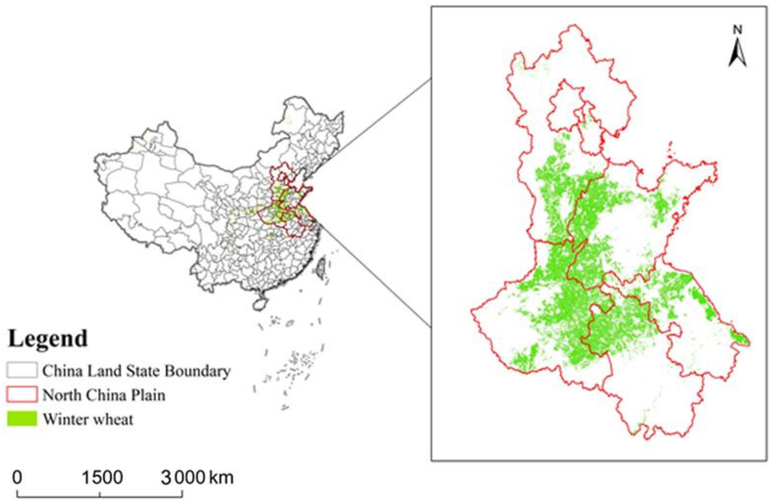
Figure 1. Winter wheat growing area in China.
Agriculture 12 00571 g001
Figure 2. Experimental flow chart (Related parameter description: Location represents spatial information, including latitude and longitude; a1…an represent partial regression coefficient; β is a random variable and a constant term; ε represents random error; Jan is short for January; Feb is short for February).
Agriculture 12 00571 g002
Figure 3. Correlations among the 10 climate variables and correlations between each climate variable and yield.
Agriculture 12 00571 g003
Figure 4. The model performance (predicted R2, RMSE) of two methods using different combinations of inputs for the whole growing season, each number representing a different input combination, which can be expressed as 1: SIF, 2: EVI, 3: Climate, 4: Location, 13: SIF + Climate, 23: EVI + Climate, 14: SIF + Location, 24: EVI + Location, 34: Climate + Location, 134: SIF + Climate + Location, 234: EVI + Climate + Location, 1234: SIF + EVI + Climate + Location.
Agriculture 12 00571 g004
Figure 5. Spatial pattern of winter wheat yield forecast in 2014: (a) RF, (b) MLR, (c) actual yield.
Agriculture 12 00571 g005aAgriculture 12 00571 g005b
Figure 6. Cumulative input effect on the model performance. In each set of figures, the left figure represents the changing trend of R2 with the increase of inputs; the figure on the right shows the changing trend of RMSE.
Agriculture 12 00571 g006
Figure 7. Independent and overlapping contributions of satellite and climate data to the model: (a) MLR, (b) RF.
Agriculture 12 00571 g007
Table 1. Details of dataset.
CategoryVariable(s)Temporal ResolutionSpatial Resolution
Crop yield and area Winter wheat yield
Winter wheat area
yearlyprefecture-level
SatelliteEVI, SIFmonthly0.05 degree
Climate
Spatial information
Precipitation (pre); wet day frequency (wet); near-surface average temperature (tmp); near-surface temperature minimum (tmn); near-surface temperature maximum (tmx); potential evapotranspiration (pet); vapour pressure (vap); air specific humidity (shum); surface downward shortwave radiation (srad); surface downward longwave radiation (lrad)
latitude (lat); longitude (lon)
monthly0.5 degree, 0.1 degree
Table 2. The validation results of “leave one-year out” experiment.
YearMLRRF
R2RMSE (kg/ha)R2RMSE (kg/ha)
20140.741100.920.91363.15
20150.611250.060.82529.11
20160.82964.750.87441.01
20170.771306.900.89491.89
20180.711527.230.83501.43
Median0.731229.970.85465.32
Publisher’s Note: MDPI stays neutral with regard to jurisdictional claims in published maps and institutional affiliations.