Micro-Investment by Tanzanian Smallholders’ in Drip Irrigation Kits for Vegetable Production to Improve Livelihoods: Lessons Learned and a Way Forward

Abstract

Food security in sub-Saharan Africa is one of the major issues confronting the continent. Innovative use of fresh water, the world’s scarcest food production resource, is vital for family-run small-holder agricultural systems, which supply up to 80% of the world’s food. Agriculture employs 70% of Tanzania’s rural population and supplies 95% of the country’s food. The goal was to measure the impact of smart drip irrigation kits on smallholder farmers’ resilience and rural poverty in Tanzania. A household survey was conducted using an exploratory sequential design in four districts (Babati, Hai, Kasulu, and Kilosa) in Tanzania. A total of 383 respondents (Micro-investing (MI) farmers, n = 195; control, n = 187) were randomly selected from a pool of 3444 farmers. Partial budgeting and enterprise economic analysis were used for the calculation of gross margins, and multivariate analysis was used for poverty analysis. Gross margin analysis showed that communities using drip-irrigated vegetable farming are more profitable. Partial budgeting analysis showed that micro-irrigation increased the revenue generation for most vegetable varieties. However, multivariate analysis was unable to confirm that household poverty was markedly reduced through the adoption of this technology. Half of the MI farmers could afford an education for their children due to the extra income generated from MI. This investment strategy has the potential to improve smallholder livelihoods and resilience to climate change.

1. Introduction

Food security is one of the main challenges for sub-Saharan African countries, where the population is expected to more than double by 2050 [1]. Food requirements are expected to increase 3-fold in this time frame. Global political and climate factors challenge farmers to remain productive and maintain the integrity of supply chains, as well as the affordability of food across the region. Innovative approaches for use of the world’s most limited resource for food production, fresh water, are critical for the future viability of family-operated pro-poor small-holder farming systems, which provide up to 80% of the world’s food [2].

Agriculture is the backbone of the Tanzanian economy, accounting for 25.8% of Tanzania’s GDP and driving the livelihoods of more than 70% of the rural population, while generating 40% of export earnings [3] and producing 95% of the country’s domestic food [4]. Tanzania’s population (approx. 59 million) is growing, and over 14 million Tanzanians live below the poverty line with few options for earning a living [5]. While severe climate affects the fragility of production systems, about 99% of Tanzania’s crops are dependent on rainfall and only 1% are irrigated [6]. The dependence on rain for agriculture emphasizes the significance of efficient and targeted water utilization for agricultural production. Drip irrigation systems make optimal use of water [7]. Drip irrigation provides a slow, even distribution of low-pressure water to the soil and plants via plastic tubing placed at the root zone of the plants. It provides an alternative to sprinkler or furrow irrigation systems. Drip irrigation can be adjusted to meet the needs of crops requiring different watering rates.

Despite the importance of agriculture for livelihood and overall development in Tanzania, the sector is characterized by smallholder subsistence farming with low productivity, over-dependence on unreliable rain-fed agriculture, and limited access to essential resources, such as seeds and fertilizers, and to contemporary technology. In addition, research-extension-farmer linkages are fragmented and often do not exist. Smallholder farming practices are now dominated, more than ever, by severe climate influences and environmental degradation [8,9,10]. The recent COVID-19 pandemic has also exacerbated vulnerabilities, especially in sectors that rely on global demand and exports (e.g., tourism and agriculture), with the current economic outlook looking uncertain [11].

Smallholders face numerous challenges along the supply chain, including pests and diseases, poor transportation and crop storage infrastructure, limited packaging and processing capacity, lack of access to technology, unfavorable financing terms, poor marketing systems, and weak quality control systems [4]. Crop production in Tanzania is centered around a few key food crops: maize, cassava, rice, potatoes (sweet and Irish), bananas, sorghum, and sugar cane [4]. The main cash crops are cashew nuts, coffee, cotton, sisal, tea, and tobacco [12].

Tanzanian supply chains are characterized by long distances between markets and producers, poor road conditions, and limited market information, which hinder the efficient flow of staple crops and vegetables from surplus-producing areas, where prices are lowest, to urban and deficit markets, where prices are high [13]. Nearly two-thirds of Tanzanian smallholder farmers sell their produce at the farm gate with very low profit margins to avoid high transportation costs to distant markets [14].

Although Tanzania currently produces sufficient food to feed its population, the poorest and most marginalized households have limited access [15]. The average cost per day for a healthy diet is USD 2.33, which is well beyond the financial means of many Tanzanians [16,17]. Chronic malnutrition rates are above average for the region, with 34% of children under five being stunted. Anemia is prevalent in children and women of reproductive age, while the incidence of obesity is increasing [15].

Improving the commercial viability of smallholder farms to alleviate domestic food shortages is vital. This study focused on investigating the viability of micro-investment in affordable drip irrigation technologies by smallholder farmers to grow vegetables.

Using this approach, farmers invest (micro-investment) in the drip irrigation kits, comprising a drip irrigation system along with the provision of seeds, fertilizers, pesticides, and ongoing technical advice for all household members throughout the growing season. The Norwegian Church Aid (NCA) has initiated this intervention by providing the drip irrigation kits to the smallholders who are responsible for repaying the cost after the crop is harvested and sold. This approach was replicated across several farmer groups to allow for specialization of crops and the opportunity to aggregate produce to establish more effective marketing opportunities.

The micro-investment kits are a market-based solution for poverty reduction, characterized as “initiatives that use the market economy to engage low-income people as clients and offering them socially good items at affordable costs” [18]. The design and content of these kits focus on resilience to climate change.

We hypothesize that the implementation of micro-investment in drip irrigation kits for vegetable production will increase the efficiency of water utilization, resulting in higher crop yields and financial returns that will improve the livelihoods of farmers and alleviate their poverty. The focus on vegetables relates to their short production season and high consumption at the local level, thus providing a ready market for any increase in production while improving the nutritional quality of the domestic food basket. The need to focus on vegetable production by smallholder farmers in sub-Saharan Africa and, more particularly, Tanzania, to improve their livelihoods is based on the intransigence of governments in the region to formulate policies to invest in agrarian reforms designed to stabilize domestic production in the face of increasing threats from climate change and world-wide political insurrection.

2. Materials and Methods

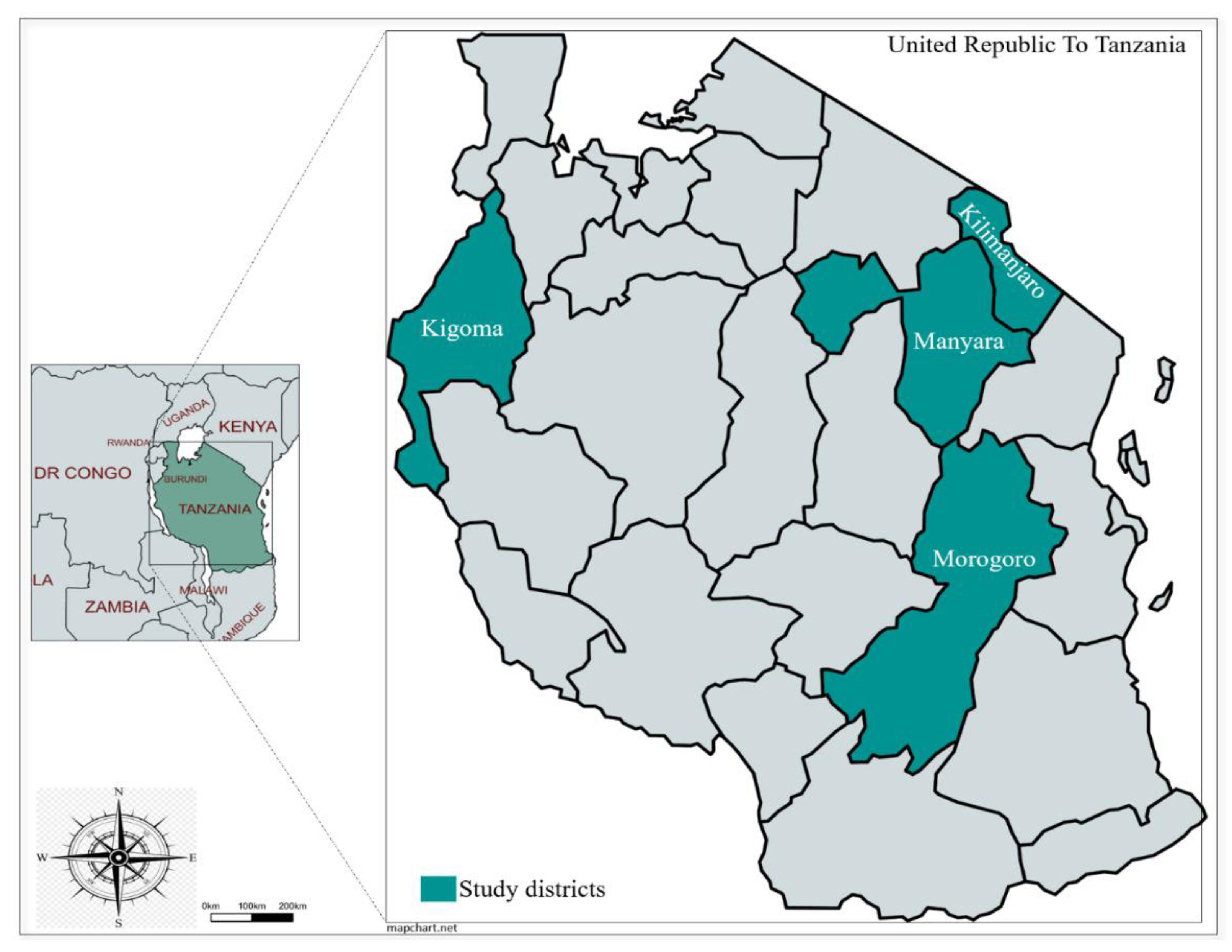
2.1. Study Design and Data Collection

A mixed-methods approach was used to generate a broad and comprehensive understanding of the impact of MI interventions. Quantitative research was implemented to understand broad patterns, while qualitative research was used to sample the experiences, attitudes, and perspectives of the farmers engaged in the program [19]. This study adopted an exploratory sequential design. This allows for a comparison between the population which has benefitted from the MI-initiative and a control group, leading to an assessment of the impact of the intervention. The statistical analysis warranted some further explanation, and qualitative interviews were conducted to explore possible reasons for the differences we found.

A cross-sectional survey was carried out in four districts (

Table 1. Distribution of sample size, micro-investing (MI) and control farmers, across four districts in Tanzania.

District	Region	MI Farmers	Control Farmers
Babati	Manyara	50	50
Hai	Kilimanjaro	51	47
Kasulu	Kigoma	50	45
Kilosa	Morogoro	45	45
Total		196	187

, Figure 1) between February–March 2021. In each study district, a closed-ended questionnaire was given to ~50 MI-farmers investing in vegetable kits (MI farmers) and ~50 control group farmers (control farmers) without MI. To maintain a balance between two groups, the number was set at a minimum of 50 farmers per group per district. The farmers were selected using a single-step cluster sampling method from a pool of 3444 registered farmers [20].

Survey: The survey consisted of questions relating to costs, economic profitability, re-investment, and poverty, based on concepts such as gender and asset ownership. The socio-economic characteristics of each group were similar in each district. The survey was pre-tested prior to data collection to assess language, content, and clarity and was revised accordingly.

The study districts were chosen to ensure socioeconomic and geographic equality of representation. In addition, NCA has started the MI-initiatives only in the study districts. The livelihood strategies for the population in these regions primarily revolve around agriculture. Data collection was carried out by NCA field staff in Tanzania, and an introduction to the questionnaire and training was provided prior to data collection.

2.2. Data Analysis

Three types of analysis were used for this study, namely, gross margin analysis, partial budgetting for economics, and multivariate analysis for poverty analysis.

Economics of Enterprises

Gross margin (GM) per bed (one bed is 15 m long, 1 m wide, and 30 cm high. The beds were spaced 50 cm away from each other and a minimum of 1.5 m away from the fence. Sunken beds were recommended during dry periods and raised during rainy periods) for both MI and control group vegetable farmers was calculated as “enterprise” income (i.e., each vegetable crop sale in 2021) less variable costs on a per bed basis [21]. Sale price, revenue, total variable cost (TVC), and GM amounts are presented in Tanzanian Shillings (TSh), where 1 USD = 2330 TSh & 1 TSh = 0.00043 USD (approximately). Yield was calculated as per bed per season. Since the sample population (MI and control) consists of pro-poor smallholder farmers, fixed costs were not calculated and were assumed to be the same for both groups. The break even value for price and yield for each enterprise commodity was calculated by the following formula:

Break even price: Total variable cost/net yield

Break even yield = Total variable cost/output price

Farmers who purchased MI kits were expected to increase their production and, thus, profitability. However, profitability may change depending on local conditions and production systems. Partial budgeting is often the appropriate way to analyze changes involving interactions between the production of different commodities within the same enterprise (crops/vegetables) [22]. It provides a formal and consistent method for calculating the expected change in profit from a proposed change in the farm business. It compares the profitability of one alternative, typically what is currently practiced traditionally, with a proposed single alternative. Throughout the discussion of the partial budgeting, the emphasis will be on changes in revenue and expenses. The result is the expected change in profit [22].

2.3. Statistical Analysis to Determine the Impact of MI on Poverty Reduction

The economic benefits accruing from the use of MI interventions can be equated with a level of poverty reduction and improved livelihoods. As a result, determining the impact of MI intervention on poverty reduction was critical. Given the multidimensional and complex nature of poverty reduction, a set of variables commonly used to measure poverty alleviation was used. These food security indicators have been validated previously and are commonly used by organizations such as FAO and the World Food Program [16,23,24,25].

Gender equality and women’s empowerment are considered essential for poverty reduction. Women’s empowerment is often defined as the “expansion in people’s ability to make strategic choices in a context where this ability was previously being denied to them” [26]. Lack of decision-making power is considered an important contributor to women’s disempowerment in agriculture and therefore is an important indicator of women’s role in control of resources [27,28]. Thus, we have used the Women’s Autonomy Index as an indicator of women’s empowerment and inequality.

SPSS was used to transform and analyze the data. The analysis was carried out in the following manner:

• Independent sample t-tests were used to compare the MI and control farmers to test for differences in the dependent variables.
• Variables for which significant differences between the MI and control farmers were apparent were analyzed further using multiple linear regression while controlling for several explanatory factors. Explanatory factors are characteristics of the sample that could potentially explain the differences seen in the dependent variables (poverty index, asset ownership index, sanitation/WASH, food consumption score, reduced coping strategies index, methods of adequate food provision, and women’s autonomy index). The following explanatory factors were included in the regression modeling: gender, age, education level, household size, market distance, farm size, livestock ownership, and ownership of farming machinery.

Statistical significance was set at α = 0.5 for all statistical tests. All the indicators are defined below:

• Poverty index: A composite index created to measure poverty at the household level. The index is constructed of nine verifiable indicators (such as household size, education, housing, cooking fuel, assets, crop farming, and livestock ownership). The score ranges from 0 (most likely below a poverty line) to 87 (least likely below a poverty line).
• Asset ownership index [29]: A proxy measure for the economic well-being of a household. The index is based on the ownership of select durable goods (table, bed, TV, mobile phone, radio, bicycle, etc.). Owned goods are summed into one composite variable, with a value between 0 (no assets) and 19.
• Sanitation/WASH [30]: A composite variable based on access to safe drinking water distanced no more than 30 min away (roundtrip, including queuing) and access to improved sanitation facilities. The variable value is between 0 (no access to safe drinking water and improved sanitation facilities) and 2 (access to both).
• Food Consumption Score (FCS) [31]: A complex indicator of household (HH) food security considering dietary diversity, food frequency, and the relative nutritional importance of different food groups. It is calculated using the household’s frequency of consumption of different foods in a seven-day period. Each food group is assigned a weight reflecting its nutrient density. The household’s food consumption status is based on the following thresholds: 0–21: Poor; 21.5–35: Borderline; >35: Acceptable.
• Reduced Coping Strategies Index (rCSI) [32]: Indirectly captures food security by measuring the frequency and severity of coping behaviors adopted by households during food shortages. Each strategy (limiting portion sizes, reducing the number of mealtimes, borrowing food, relying on relatives, relying on cheaper food, and restricting consumption) is given a different weighting. The higher the sum, the lower the food security.
• Months of Adequate Household Food Provision (MAHFP) [33]: Measures the duration of a period during the last year where the household was able to access sufficient food to meet their needs. This is used as a proxy measure of household food access.
• Women’s Autonomy Index (WAI) [30]: Measures the women’s autonomy manifested through key dimensions (access to income, mobility, and freedom of expression). The value ranges between 0–1, where 1 is the highest autonomy.

3. Results and Discussion

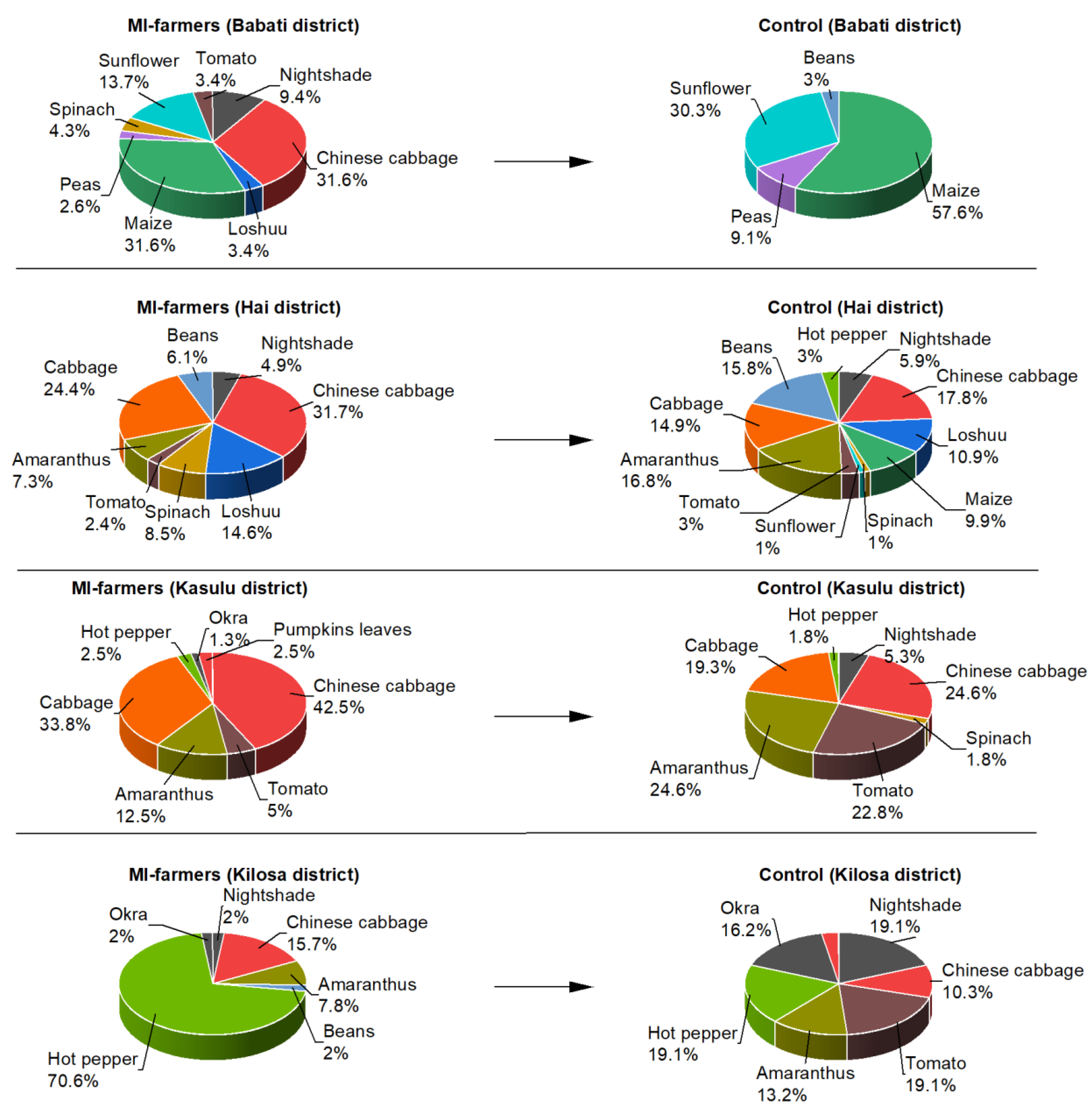
3.1. Demographic and Socioeconomic Data

There were a few significant differences between the two groups when the means for the four study sites were compared. Firstly, the mean household size was higher in the MI group (5.77 vs. 5.21, p = 0.012). A higher number of females was also found in the MI group (70.4% vs. 56.7%, p = 0.007). This is perhaps not surprising, given that women were a key target group of the MI program. Lastly, MI farmers produced more food crops (2.41 vs. 1.93, p = <0.001).

The vegetables grown by the farmers in the sample included Chinese cabbage, cabbage, African eggplant, African nightshade, tomato, hot pepper, and pawpaw, while the most commonly owned livestock were cattle and chickens. Most respondents reported owning their land, and only a small portion rented land. The average distance to the nearest reliable market was 2.21 km for the MI farmers and 1.83 km for the control farmers in all four districts. Of note was the large distance to the nearest market in the Kilosa district (registered = 4.40 and control = 4.20 km) compared to the other study sites.

Since the main target groups for the MI intervention were the poorest small-holders, women, and youth, it was important to report the distribution of MI farmers by gender and age.

Table 2. Demographic, socioeconomic, and farm characteristics of the MI farmers and the control farmers in the different study districts.

	MI Farmers					Control Farmers a					p-Value
	Babati	Hai	Kasulu	Kilosa	Total	Babati	Hai	Kasulu	Kilosa	Total
Mean age (M ± SD)	44.16	42.02	38.66	43.40	42.03	39.10	35.77	45.87	38.98	39.67	0.088
	(12.26)	(10.21)	(14.17)	(9.82)	(11.88)	(15.74)	(7.83)	(12.14)	(12.52)	(13.14)
Gender (%)											0.007 **
Male	48.0	17.6	30.0	22.8	29.6	38.0	66.0	15.6	51.1	42.8
Female	52.0	82.4	70.0	77.8	70.4	62.0	34.0	84.4	48.9	56.7
Mean household size (M ± SD)	6.37	4.84	6.36	5.53	5.77	5.28	4.17	6.49	4.91	5.21	0.012 *
	(2.03)	(2.03)	(2.44)	(1.78)	(2.17)	(2.11)	(1.85)	(2.26)	(2.02)	(2.21) *
Education (%)											0.166
Illiterate	14.0	0	6.0	2.2	5.6	10.0	0	15.6	0	6.4
Primary	58.0	64.7	64.0	71.1	54.1	64.0	53.2	77.8	62.2	64.2
Secondary	16.0	25.5	18.0	20.0	30.1	18.0	34.0	4.4	26.7	20.9
University/College	12.0	7.8	12.0	6.7	9.7	8.0	12.8	2.2	11.1	8.6
Farm size, acers b (M ± SD)	4.66	1.99	3.81	1.16	2.94	4.85	2.15	3.23	0.74	2.80 (4.50)	0.744
	(6.88)	(1.99)	(4.19)	(1.27)	(4.42)	(7.36)	(2.89)	(2.25)	(1.32)
Market distance, km (M ± SD)	2.43	1.18	1.21	4.42	2.21	1.01	1.07	1.57	4.40	1.83
	(3.20)	(0.67)	(0.58)	(5.08)	(3.15)	(1.12)	(1.50)	(0.51)	(5.25)	(2.81)
Food crop production (no. of crops produced) (M ± SD)	3.86	2.10	2.26	1.27	2.41	1.80	2.32	1.51	2.04	1.93	<0.001 ***
	(1.83)	(0.81)	(1.41)	(0.75)	(1.58)	(1.11)	(0.91)	(0.59)	(0.88)	(0.93)
Livestock ownership (%)	94.0	37.3	54.0	70.5	63.3	88.0	31.9	64.4	71.1	64.2	0.906
Access to farming machinery (yes/no) (%)	6.0	0	0	22.2	6.6	4.0	2.1	0	20.0	6.4	0.932

^a. Six control farmers did not engage in crop farming, but owned livestock. ^b. includes owned and rented land. *, ** and *** denote statistical significance at p < 0.05, p < 0.01, and p < 0.001 levels, respectively.

provides this information for the MI and control farmers. The proportion (%) of MI and control farmers growing crops is shown in Figure 2.

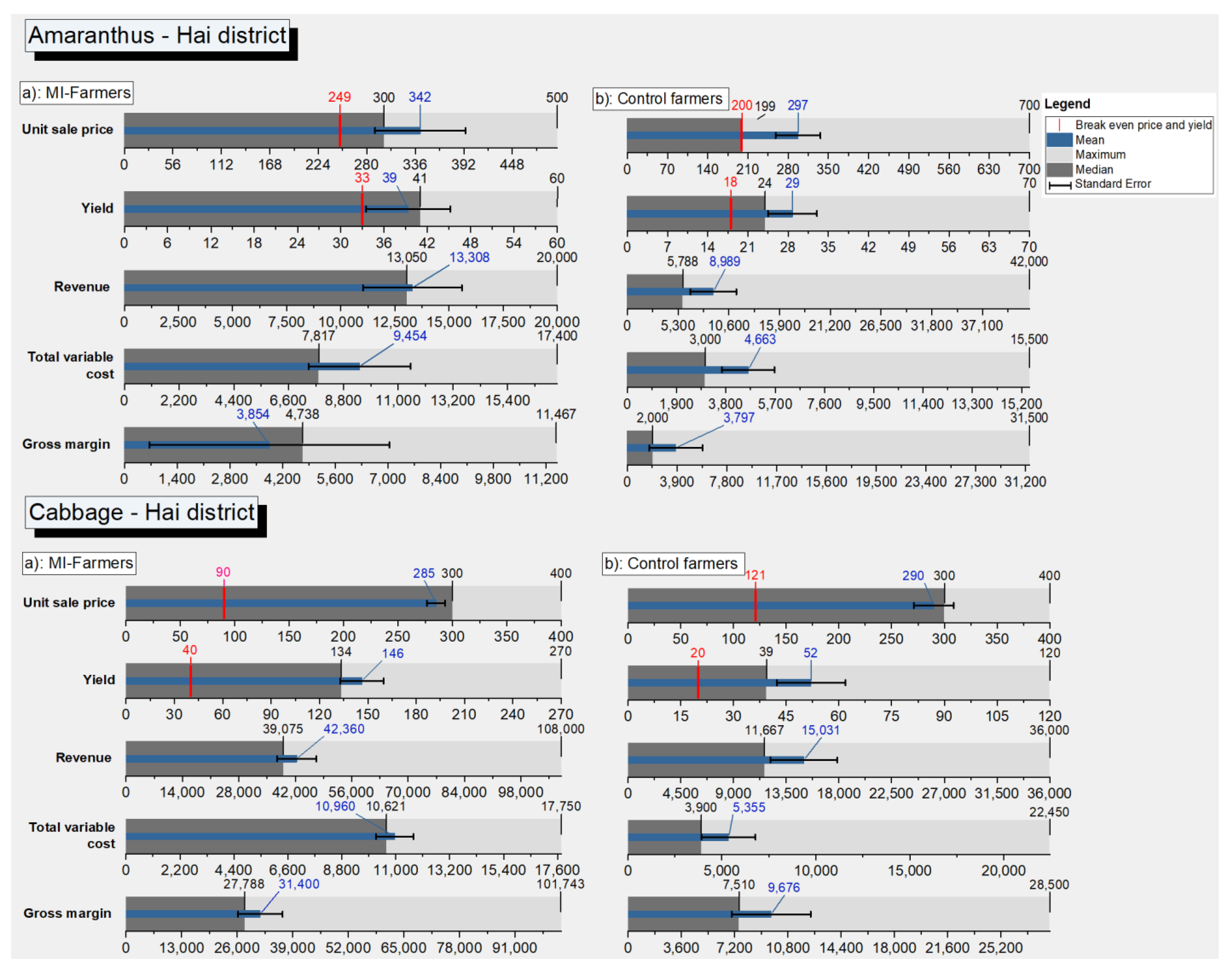
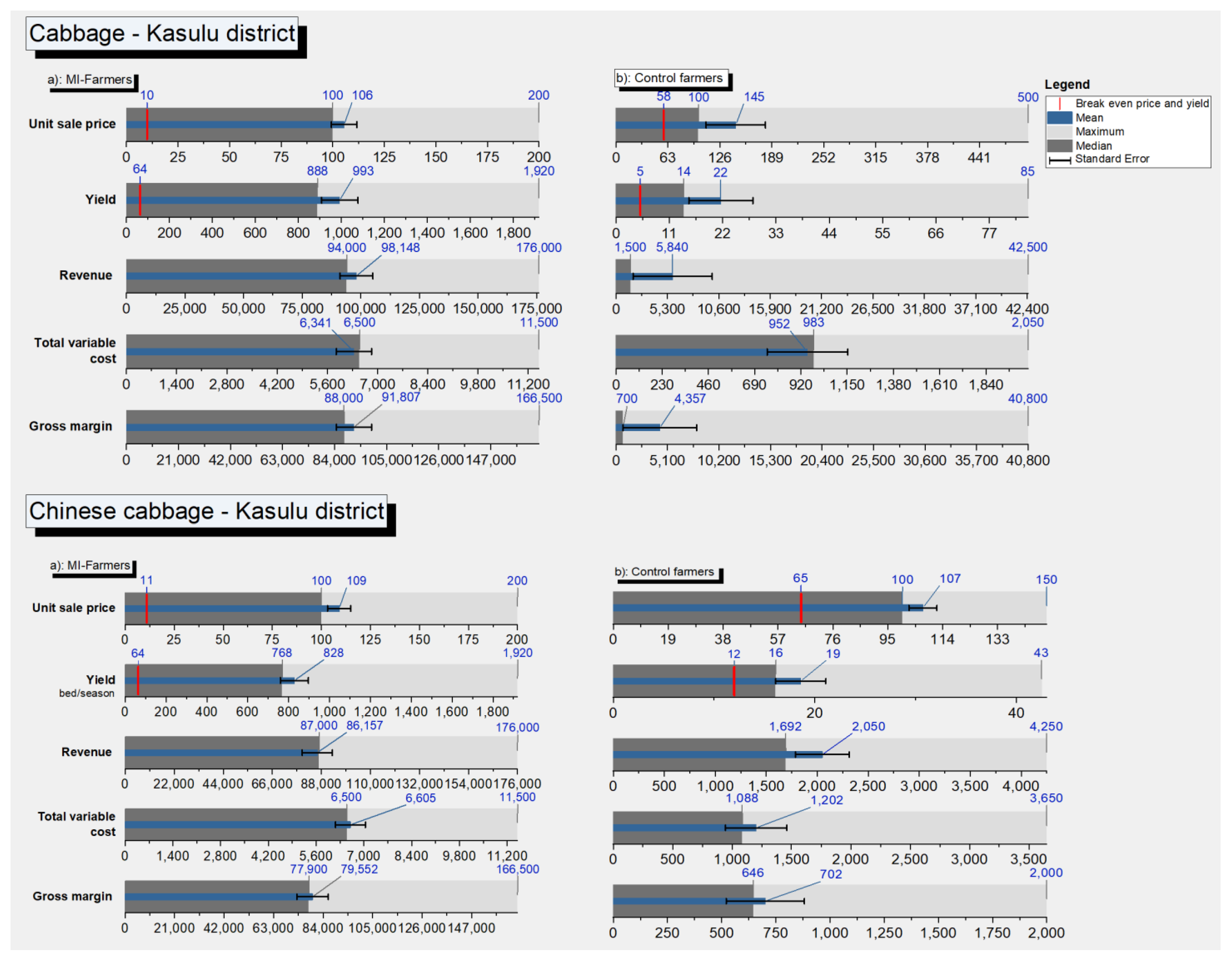
3.2. Economic Analysis—Partial Budgeting

3.2.1. Economic Assessment of Specific Districts and Vegetables

The net yield, sale price, total variable cost (TVC), revenue, and gross margin (GM) per bed were calculated for both MI and control farmers in the Hai district (growing Amaranthus, cabbage, and Loshuu), Kasulu district (growing Amaranthus, cabbage, Chinese cabbage, and tomatoes), and Kilosa district (growing Amaranthus, Chinese cabbage, hot peppers, and pawpaw) (Figure 3, Figure 4, Figure 5, Figure 6, Figure 7 and Figure 8). The comparison in terms of income from vegetable production between MI and control farmers was not possible for the Babati district since control farmers only grew cash crops (Figure 2) while MI farmers were only growing vegetables. Figure 3, Figure 4, Figure 5, Figure 6, Figure 7 and Figure 8 show the enterprise comparison of MI and control farmers across the three districts.

3.2.2. Hai District Farmers Economic Analysis

The values for unit sale price, yield, revenue, TVC, and GM were greater for MI than for control farmers for all commodities (Amaranthus, cabbage, and Loshuu) except for cabbage, where both MI and control farmers earned the same unit sale price. Figure 3 and Figure 4 show a detailed comparison of unit break-even price and yield, selling price, yield, revenue, TVC, and GM.

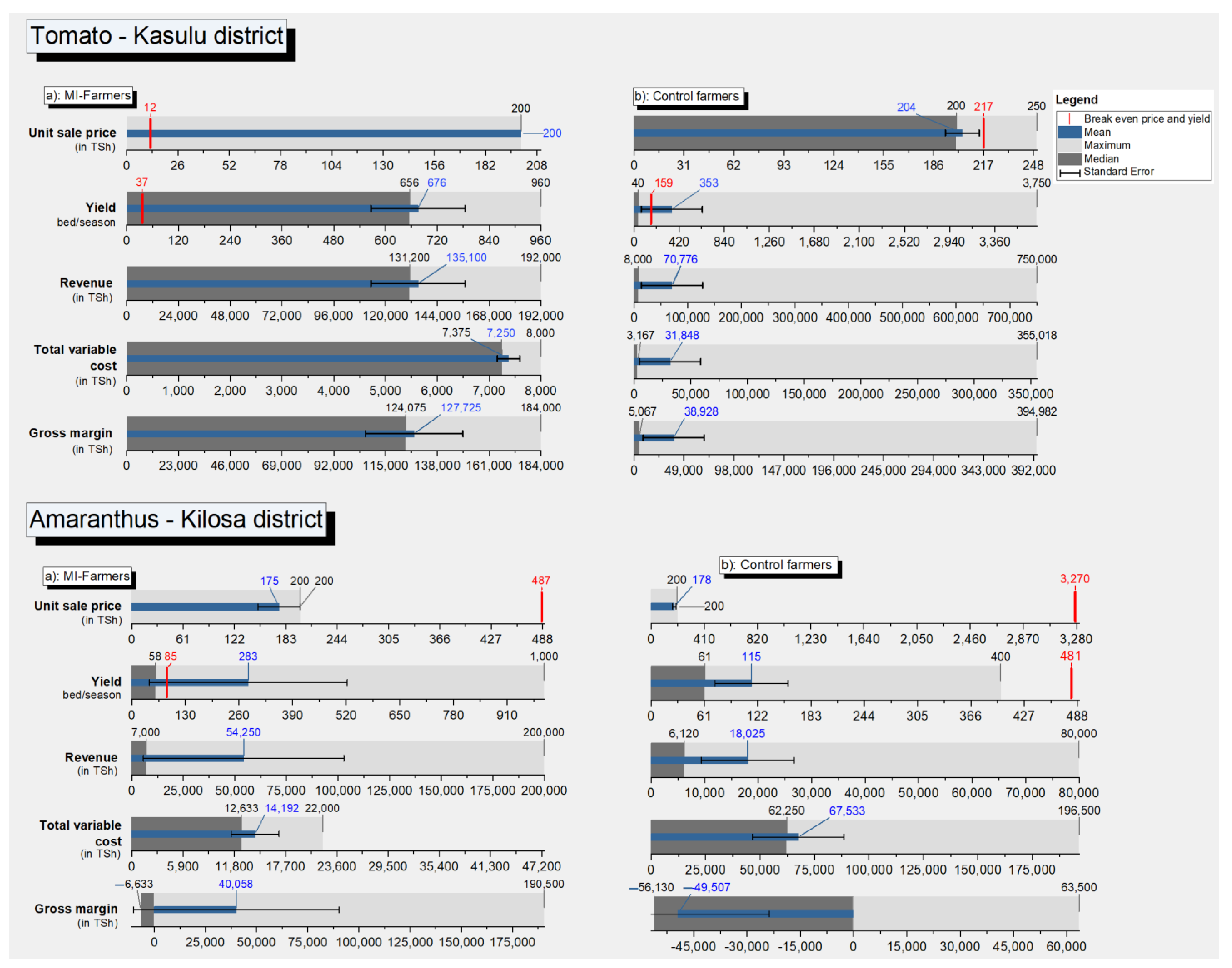
3.2.3. Kasulu District Farmers Economic Analysis

MI farmers achieved greater values for yield, revenue, TVC, and GM than control farmers did. However, when compared to the control farmers, MI farmers received a lower unit sale price for cabbage and an equivalent sale price for Chinese cabbage and tomatoes. Figure 4, Figure 5 and Figure 6 show a detailed comparison of unit break-even price and yield, selling price, yield, revenue, TVC, and GM.

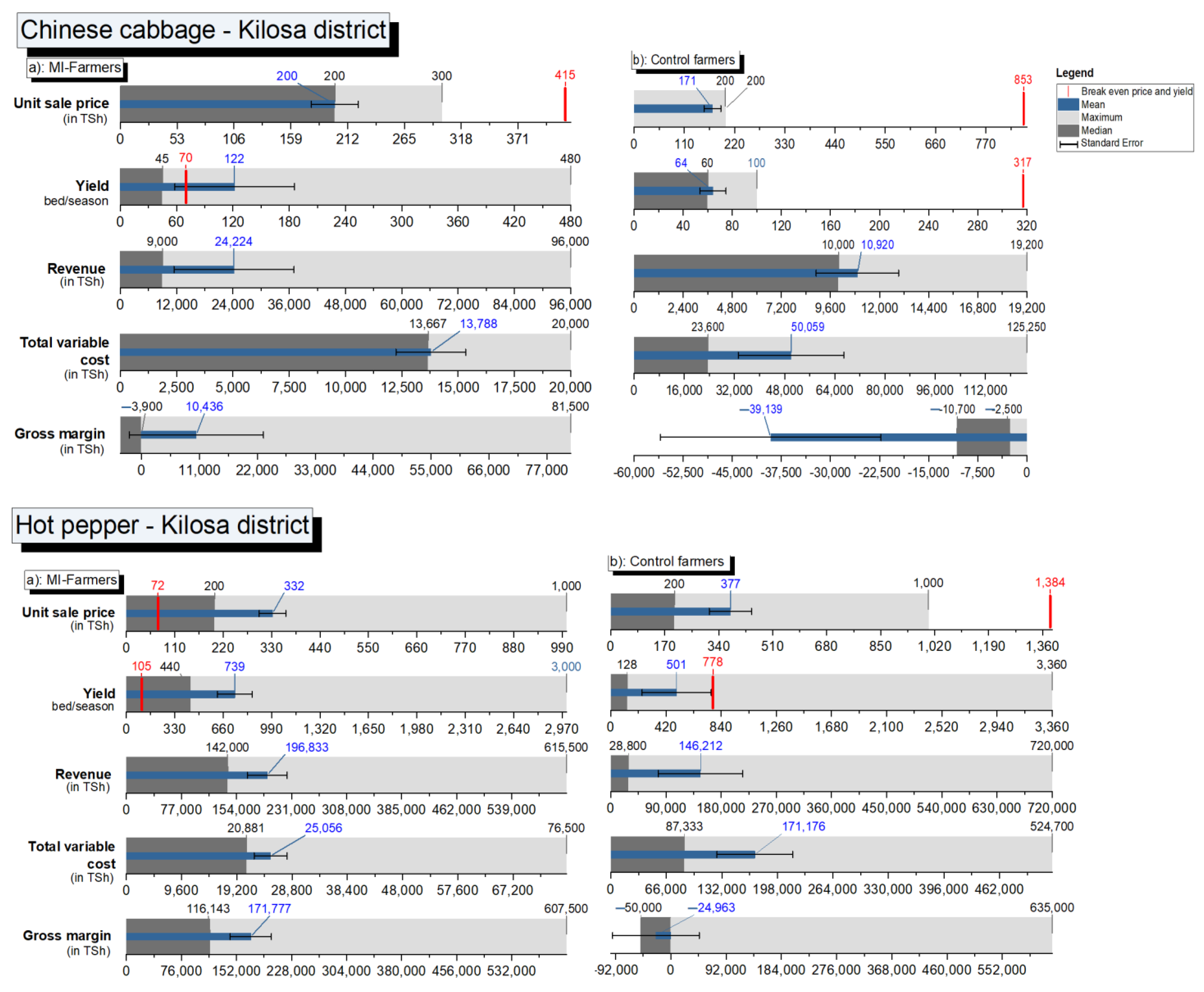
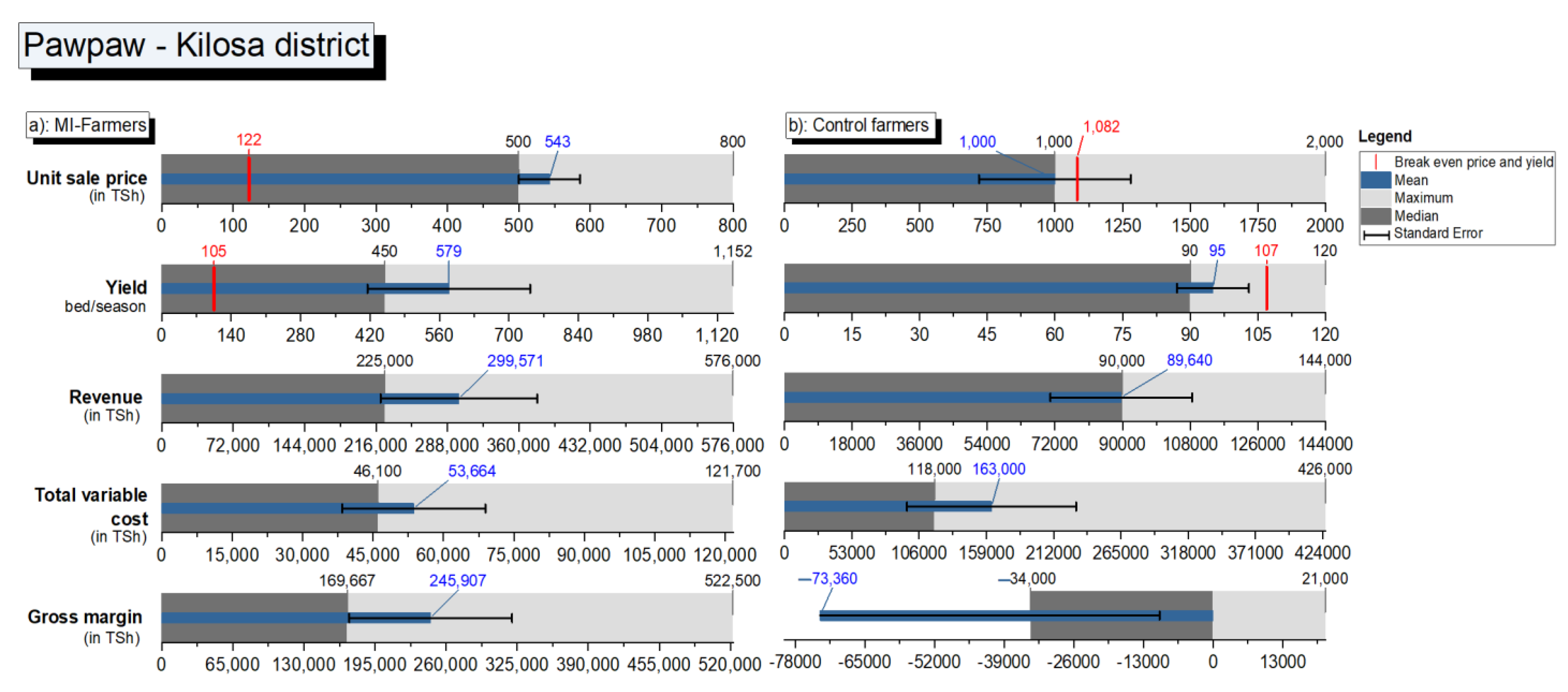
3.2.4. Kilosa District Farmers Economic Analysis

MI farmers had higher yields, revenue, and GM values than control farmers. However, the unit sale price gained by MI farmers was comparable to the control farmers for Amaranthus and was lower for hot peppers and pawpaw. When compared to MI farmers who do not hire any labor, most control farmers reported hiring labor for farm operations, which boosted their TVC. Figure 6, Figure 7 and Figure 8 show a detailed comparison of unit break-even price and yield, selling price, yield, revenue, TVC, and GM.

Although greater yields and unit sales prices resulted in higher GMs, TVC was higher for control farmers in the Kilosa area, resulting in negative GMs. Higher yields were recorded for MI farmers across all districts and commodities, but unit pricing impacted the GMs for vegetables in the Kilosa district especially.

The results of gross margin analysis showed that vegetable yield has increased, as reported by other studies [34]. Increased yield with efficient water use (less evaporation) helps improve smallholder livelihoods. However, a higher per unit price is vital to increase the overall gross margin for the produce. Therefore, collective action is vital for gaining proper market access for smallholder produce [35].

Micro-investing (MI) and control farmer comparison growing Amaranthus and cabbage in the Hai district (Figure 3):

Amaranthus: The average net yield for MI farmers was higher (mean: 39 vs. 29 bunches/bed). The mean sale price per bunch was slightly higher for the MI farmers (342 vs. 297 TSh/bunch). The break even price (TSh/bunch) and yield (bunches/bed/season) for the MI and control farmers were 249 vs. 200 and 33 vs. 18, respectively. The average revenue per bed was higher (13,308 TSh/bed/season) for the MI farmers compared with the control farmers (8989 TSh/bed/season). On an average, total variable cost per bed was higher for the registered farmers (9454 vs. 4663 TSh/bed/season) compared to control farmers. The average value of gross margin/bed calculated for the registered farmers was slightly higher (3854 vs. 3797 TSH/bed). In conclusion, comparing average values with control farmers, registered farmers have gained a slightly higher net yield per bed season, a slightly higher sale price, higher revenue, and also higher variable costs, resulting in a similar gross margin (3854 vs. 3797 TSh/bed/season) for the enterprise.

Cabbage: The average net yield for MI farmers was higher (mean: 146 vs. 52 bunches/bed/season). However, there was not a big difference in the mean sale price per bucket for the MI and control farmers (285 vs. 290 TSh/bunch). The break even price (TSh/bucket) and yield (kg/bed/season) for the MI and control farmers were 90 vs. 121 and 40 vs. 20, respectively. The average revenue per bed was higher (42,360 TSh/bed/season) for the MI farmers compared with the control farmers (15,031 TSh/bed/season). On average, total variable cost per bed was higher for the registered farmers (10,960 vs. 5355 TSh/bed/season) compared to control farmers. The average value of gross margin/bed calculated for the registered farmers was significantly higher (31,400 vs. 9676 TSH/bed). In conclusion, comparing average values with control farmers, registered farmers have gained a significantly higher yield, although at a lower sale price, resulting in a higher average gross margin for the enterprise.

Micro-investing (MI) and control farmer comparison growing Loshuu in Hai district and Amaranthus in Kasulu district (Figure 4):

Loshuu: The average net yield for MI farmers was higher (mean: 201 vs. 93 bunches/bed). The mean sale price per bunch was higher for the MI farmers (388 vs. 327 TSh/bunch). The break-even price (TSh/bunch) and yield (bunches/bed/season) for the MI and control farmers were 78 vs. 161 and 35 vs. 35, respectively. The average revenue per bed was higher (84,079 TSh/bed/season) for the MI farmers compared with the control farmers (32,275 TSh/bed/season). On average, the total variable cost per bed was slightly higher for the registered farmers (12,990 vs. 11,179 TSh/bed/season) compared to the control farmers. The average value of gross margin/bed calculated for the registered farmers was significantly higher (71,089 vs. 21,096 TSH/bed). In conclusion, comparing average values with control farmers, registered farmers have achieved a higher net yield per bed season, a slightly higher sale price, higher revenue, and also slightly higher variable costs, resulting in a high gross margin for the enterprise.

Amaranthus: The average net yield for MI farmers was significantly higher (mean: 555 vs. 27 bunches/bed/season). The mean sale price per bunch was higher for the MI farmers (165 vs. 114 TSh/bunch) compared with the control farmers. The break-even price (TSh/bucket) and yield (kg/bed/season) for the MI and control farmers were 10 vs. 57 and 31 vs. 15, respectively. The average revenue per bed was significantly higher (89,330 TSh/bed/season) for the MI farmers compared with the control farmers (3007 TSh/bed/season). On average, the total variable cost per bed was higher for the registered farmers (4800 vs. 1498 TSh/bed/season) compared to the control farmers. The average value of gross margin/bed calculated for the registered farmers was significantly higher (84,530 vs. 1293 TSH/bed). In conclusion, registered farmers have gained significantly higher yield and sale price than control farmers, resulting in a higher average gross margin for the enterprise.

Micro-investing (MI) and control farmer comparison growing cabbage and Chinese cabbage in the Kasulu district (Figure 5):

Cabbage: The average net yield for MI farmers was higher (mean: 993 vs. 22 bunches/bed). The mean sale price per bunch was lower for the MI farmers (106 vs. 145 TSh/bunch). The break even price (TSh/bunch) and yield (bunches/bed/season) for the MI and control farmers were 10 vs. 58 and 64 vs. 5, respectively. The average revenue per bed was much higher (98,148 TSh/bed/season) for the MI farmers compared with the control farmers (5840 TSh/bed/season). On average, total variable cost per bed was higher for the registered farmers (6341 vs. 952 TSh/bed/season) compared to control farmers. The average value of gross margin/bed calculated for the registered farmers was significantly higher (91,807 vs. 4357 TSH/bed). In conclusion, comparing average values with control farmers, registered farmers have gained a higher net yield per bed season, but at a lower sale price, higher revenue, and also slightly higher variable costs, resulting in a high gross margin for the enterprise.

Chinese cabbage: The average net yield for MI farmers was significantly higher (mean: 828 vs. 19 bunches/bed/season). The mean sale price per bunch was similar for the MI farmers (109 vs. 107 TSh/bunch) compared with control farmers. The break even price (TSh/bucket) and yield (kg/bed/season) for the MI and control farmers were 11 vs. 65 and 64 vs. 12, respectively. The average revenue per bed was significantly higher (86,157 TSh/bed/season) for the MI farmers compared with the control farmers (2050 TSh/bed/season). On average, total variable cost per bed was higher for the registered farmers (6605 vs. 1202 TSh/bed/season) compared to control farmers. The average value of gross margin/bed calculated for the registered farmers was significantly higher (79,552 vs. 702 TSH/bed). In conclusion, comparing average values with control farmers, registered farmers have gained a significantly higher yield, although similar sale price, compared with control farmers, resulting in a higher average gross margin for the enterprise

Micro-investing (MI) and control farmer comparison growing tomatoes in the Kasulu district and Amaranthus in the Kilosa district (Figure 6):

Tomato: The average net yield for MI farmers was higher (mean: 676 vs. 353 bunches/bed). The mean sale price per bunch was similar for the MI farmers (200 vs. 204 TSh/bunch). The break-even price (TSh/bunch) and yield (bunches/bed/season) for the MI and control farmers were 12 vs. 217 and 37 vs. 159, respectively. The average revenue per bed was much higher (135,100 TSh/bed/season) for the MI farmers compared with the control farmers (14,174 TSh/bed/season). On average, total variable cost per bed was higher for the MI farmers (7375 vs. 4917 TSh/bed/season) compared to the control farmers. The average value of gross margin/bed calculated for the registered farmers was significantly higher (127,725 vs. 9257s TSH/bed). Although the cost was higher for the MI farmers, significantly higher yields were reported by the MI farmers compared to the control farmers, which benefited the MI farmers. In conclusion, registered farmers have gained a higher net yield per bed season but a similar sale price and higher revenue than control farmers. Yet, they incurred slightly higher variable costs, resulting in a high gross margin for the enterprise.

Amaranthus: The average net yield for MI farmers was significantly higher (mean: 283 vs. 115 bunches/bed/season). The mean sale price per bunch was similar for the MI farmers (175 vs. 178 TSh/bunch) compared with the control farmers. The break even price (TSh/bucket) and yield (kg/bed/season) for the MI and control farmers were 487 vs. 3270 and 85 vs. 481, respectively. The average revenue per bed was significantly higher (54,250 TSh/bed/season) for the MI farmers compared with the control farmers (18,025 TSh/bed/season). On average, total variable cost per bed was lower for the registered farmers (14,192 vs. 67,533 TSh/bed/season) compared to control farmers due to higher contractual labor costs for the control farmers. The average value of gross margin/bed calculated for the registered farmers was significantly higher (40,058 vs. −49,507 TSH/bed). In conclusion, registered farmers have gained a significantly higher yield, although at a similar sale price, compared with control farmers, resulting in a higher average gross margin for the enterprise.

Micro-investing (MI) and control farmer comparison growing Chinese cabbage and hot peppers in the Kilosa district (Figure 7):

Chinese cabbage: The average net yield for MI farmers was higher (mean: 122 vs. 64 bunches/bed). The mean sale price per bunch was higher for the MI farmers (200 vs. 171 TSh/bunch). The break even price (TSh/bunch) and yield (bunches/bed/season) for the MI and control farmers were 415 vs. 853 and 70 vs. 317, respectively. The average revenue per bed was much higher (24,224 TSh/bed/season) for the MI farmers compared with the control farmers (10,920 TSh/bed/season). On average, the total variable cost per bed was lower for the MI farmers (13,788 vs. 50,059 TSh/bed/season) compared to the control farmers due to the higher cost of water purchased and contractual labor at the farms. The average value of gross margin/bed calculated for the registered farmers was significantly higher (10,436 vs. −39,139 TSH/bed). In conclusion, comparing average values with the control farmers, registered farmers have gained a higher net yield per bed season, but a similar sale price and higher revenue, and also slightly higher variable costs, resulting in a high gross margin for the enterprise.

Hot pepper: The average net yield for MI farmers was significantly higher (mean: 739 vs. 501 buckets/bed/season). The mean sale price per bunch was lower for the MI farmers (332 vs. 377 TSh/bucket) compared with control farmers. The break even price (TSh/bucket) and yield (kg/bed/season) for the MI and control farmers were 72 vs. 1384 and 105 vs. 778, respectively. The average revenue per bed was significantly higher (196,833 TSh/bed/seasson) for the MI farmers compared with the control farmers (146,212 TSh/bed/season). On average, total variable cost per bed was lower for the registered farmers (25,056 vs. 171,176 TSh/bed/season) compared to control farmers due to higher contractual labor costs for the control farmers. The average value of gross margin/bed calculated for the registered farmers was significantly higher (171,777 vs. −24,963 TSH/bed). In conclusion, comparing average values with control farmers, registered farmers have gained significantly higher yields, although at lower sale prices, compared with control farmers, resulting in a higher average gross margin for the enterprises.

Micro-investing (MI) and control farmer comparison growing pawpaw in the Kilosa district (Figure 8):

Pawpaw: The average net yield for MI farmers was higher (mean: 579 vs. 95 pieces/bed). The mean sale price per bunch was lower for the MI farmers (543 vs. 1000 TSh/piece). The break-even price (TSh/piece) and yield (pieces/bed/season) for the MI and control farmers were 122 vs. 1082 and 105 vs. 107, respectively. The average revenue per bed was much higher (299,571 TSh/bed/season) for the MI farmers compared with the control farmers (89,640 TSh/bed/season). On an average, total variable cost per bed was lower for the MI farmers (53,664 vs. 163,000 TSh/bed/season) compared to control farmers due to the higher cost of water purchased and the contractual labor at the farms. The average value of gross margin/bed calculated for the registered farmers was significantly higher (245,907 vs. −73,360 TSH/bed). Thus, registered farmers have gained a higher net yield per bed per season, but a lower sale price, higher revenue, and also slightly higher variable costs, resulting in a high gross margin for their enterprises relative to the controls.

3.2.5. Partial Budgeting

The economic data from the MI and control farmers were compared using partial budgeting analysis. The values of various vegetables from the Hai (Amaranthus, cabbage, and Loshuu), Kasulu (Amaranthus, cabbage, Chinese cabbage, and tomatoes), and Kilosa districts (Amaranthus, Chinese cabbage, hot peppers, and pawpaw) are presented in

Table 3. Partial budgeting analysis of selected vegetables grown by both MI and control group farmers (in Tanzanian shilling) in three study districts in Tanzania. (Numbers are in 1000 TSh).

Effect of Veggie-Kits on Farm Profitability, Compared with Traditional Practices (Registered vs. Control) in Three Study Districts
Districts	Hai			Kasulu				Kilosa
Vegetables	Amaranthus	Cabbage	Loshuu	Amaranthus	Cabbage	Chinese Cabbage	Tomato	Amaranthus	Chinese Cabbage	Hot Pepper	Pawpaw
Added income due to change
Increased income	4.3	27.3	51.8	86.3	92.3	84.1	120.9	36.2	13.3	50.6	209.9
Added costs due to change
Added cost product total	4.7	5.6	1.8	1.4	5.3	5.4	2.4
Reduced costs due to change
Reduced cost per season								53.3	36.2	146.1	46.3
Reduced income due to change
Reduced income
Increase in Net Income	4.3	27.3	51.8	86.3	92.3	84.1	120.9	89.5	49.5	196.7	256.2
Decrease in Net Income	4.7	5.6	1.8	1.4	5.3	5.4	2.4	0	0	0	0
Change in Net Income	−0.4	21.7	49.9	84.8	86.9	78.7	118.4	89.5	49.5	196.7	256.2

.

MI farmers recorded a positive change in net income (Table 3) except for the Amaranthus in the Hai district. The reason for this loss was higher TVC (cost of fertilizer, chemicals, seeds, and water purchased). The crop yields of MI farmers were higher than those of the control farmers (39 vs. 29 bunches per bed). The detailed explanation of all costs (added or reduced) and incomes (gained or lost) due to the micro-investment in drip irrigation is shown in Table 3.

3.2.6. Irrigation Methods Used and Distance to Nearest Market

The difficulty of engaging with appropriate control groups to determine the effect of the irrigation intervention is highlighted by these findings. In many cases, including our study, control farmers adopted the same techniques as the MI farmers. Control farmers also had less distance to transport produce to the nearest market (1.83 (±SD 2.81) vs. 2.21 (±SD 3.15) km). Most MI farmers (85%) reported that buyers collected farm produce at the farm gate.

3.3. Effect of MI on Poverty Reduction, Gender and Food Security

This section presents the results from the statistical analysis of the impact of MI on poverty.

Table 4. Mean differences in poverty indicators between registered and control group farmers.

Indicators	Registered	Control	p-Value
	M (±SD)
Poverty Index—High value desirable (0–87)	41.98 (15.39)	44.80 (16.88)	0.089
Asset Ownership—High value desirable (0–19)	6.73 (3.12)	6.27 (2.95)	0.16
Sanitation—High value desirable (Range: 0–2)	1.33 (0.69)	1.22 (0.74)	0.15
Food Consumption Score (FCS)—High value desirable (0–122) 1	60.77 (17.77)	61.69 (18.09)	0.62
Reduced Coping Strategies Index (rCSI)—Low value desirable (0–56)	9.52 (9.25)	8.96 (10.28)	0.58
Months of Adequate Household Food provision (MAHFP)—High value desirable (Range: 0–12)	10.04 (1.91)	9.85 (2.61)	0.44
Women’s Autonomy Index (WAI)—High value desirable (Range: 0–1)	0.60 (0.26)	0.53 (0.27)	0.04 *

Note: Figures are means with standard deviation in parenthesis; * denote statistical significance at p < 0.05 levels. ¹ >35 is considered acceptable according to the World Food Program.

shows the mean differences between poverty indicators, including food security of the MI and control households. Overall, for all districts, there was no significant (p = 0.05) difference between MI and control farmers for the poverty index utilized, for asset ownership, sanitation, food consumption score, the reduction in coping strategies index, and months of adequate household food provision (Table 4). However, the Women’s Autonomy Index (WAI) was significantly higher (p = 0.05) for the MI farmers.

It is important to note that during qualitative interviews, half of the respondents (MI-farmers) noted that they have used their increased income for school-related expenditures (e.g., books, uniforms, and bus fares). While more qualitative data are needed to evaluate the impact of this investment in irrigation on poverty reduction, it is possible that the intervention may lead to a long-term positive impact on the household budget and on poverty reduction.

The use of improved sanitary facilities and safe access to drinking water are important determinants of health. The only significant difference in sanitation facilities was found in Kasulu, where the usage of improved facilities and access to safe drinking water was significantly higher for the MI farmers compared with the control farmers.

Food insecurity: It is an important indicator of poverty. When individuals living in poverty improve their family income, they can increase their spending on additional food items. As such, improvements in a household’s food security are important indicators of poverty reduction. However, no significant differences in food security indicators (Food Consumption Score, FCS) were recorded between control and MI farmers (60.77 vs. 61.69). However, it is important to note that these values exceed the WFP defined acceptable threshold (<35).

For the Reduced Coping Strategies Index (rCSI) indicator, where a low score is desirable, the results are mixed. In Babati, control farmers engage in negative coping strategies, as defined by the rCSI, significantly more than MI farmers (p = 0.006). However, in Kasulu, the results show that MI farmers engage less frequently in negative coping strategies (p = 0.001). In Hai and Kilosa, no significant differences were found between the control and MI farmers. Similar results were found regarding the Months of Adequate Household Food Provision (MAHFP) indicators, in which MI farmers in Babati recorded longer periods of adequate household food provisioning (p = 0.028), while in Kasulu, the result was the opposite (p = 0.002). Again, no significant differences were found between the control and MI farmers in Hai and Kilosa. The details are provided in Appendix A. Several respondents indicated in interviews that they have experienced an increase in food production since they joined the program and therefore have extra food for storage purposes. This element of food security is not adequately covered by any of the indicators studied through this evaluation.

Nutritional diversity is another important indicator of food security. The data presented in

Table 5. Difference in food group consumption—MI and control group—mean number of days in a week when household members consumed a particular food group.

	MI-Farmers	Control	p-Value
	M (±SD)	M (±SD)
Cereals	6.59 (1.18)	6.50 (1.55)	0.538
Pulses	4.55 (1.96)	4.97 (2.01)	0.122
Vegetables	5.71 (1.80)	5.54 (1.91)	0.309
Fruit	3.58 (2.48)	3.30 (2.59)	0.280
Meat, fish, eggs	2.07 (1.69)	2.13 (1.94)	0.756
Dairy products	2.69 (2.48)	2.77 (2.73)	0.764
Sugar and honey	4.74 (2.81)	4.70 (2.92)	0.904
Oil, fats, butter	5.83 (2.11)	6.00 (2.19)	0.437

indicates whether there are significant differences in the consumption of food groups between the control and MI farmers. For both groups, there was a low consumption of fruit, meat, fish, eggs, and dairy, which means that the study participants consumed a diet that was based highly on starchy foods, carbohydrates, pulses, and vegetables. The data indicate that there are no significant differences in the consumption of cereals, vegetables, meat, fish, and eggs between the control and MI farmers across all districts.

Other farmers indicated in interviews that they were able to start farming livestock as well as buy additional land and diversify their crop production from their increased profit. This may lead to long-term positive impacts on food security.

A breakdown of the rCSI variable is provided in

Table 6. Food security in MI and control households, measured using Reduced Coping Strategies Index (rCSI).

		MI-Farmers	Control	p-Value
In the past seven days, how many days has your household had to…		M (±SD)
…rely on less preferred and/or less expensive food	All districts	3.01 (2.43)	2.61 (2.48)	0.115
	Babati	4.50 (2.58)	4.98 (2.54)	0.351
	Hai	0.90 (1.08)	0.68 (1.20)	0.340
	Kasulu	3.22 (2.43)	1.57 (1.81)	<0.001 ***
	Kilosa	3.51 (1.96)	3.02 (1.55)	0.193
…borrow food, or rely on help from a friend or relative	All districts	0.88 (1.26)	0.58 (1.33)	0.016 *
	Babati	0.78 (1.08)	0.84 (1.41)	0.811
	Hai	0.02 (0.14)	0.06 (0.32)	0.375
	Kasulu	1.48 (1.53)	0.30 (0.83)	<0.001 ***
	Kilosa	1.29 (1.31)	1.11 (1.30)	0.520
…limit portion size at mealtimes	All districts	1.04 (1.49)	1.22 (1.83)	0.279
	Babati	0.78 (1.43)	1.96 (2.60)	0.006 **
	Hai	0	0.13 (0.65)	0.183
	Kasulu	1.42 (1.77)	0.82 (1.19)	0.060
	Kilosa	2.07 (1.18)	1.93 (1.48)	0.638
…restrict consumption by an adult in order for small children to eat	All districts	0.78 (1.31)	0.96 (1.76)	0.251
	Babati	0.52 (1.27)	1.68 (2.54)	0.005 **
	Hai	0	0.06 (0.44)	0.323
	Kasulu	1.04 (1.60)	0.75 (1.30)	0.342
	Kilosa	1.64 (1.13)	1.29 (1.53)	0.214
…reduce the number of meals eaten in a day	Babati	1.38 (1.82)	1.12 (1.71)	0.153
	Hai	1.12 (1.90)	1.50 (2.16)	0.353
	Kasulu	0.06 (0.24)	0.09 (0.58)	0.768
	Kilosa	2.50 (2.03)	1.20 (2.00)	0.002 **
		1.93 (1.45)	1.71 (1.16)	0.425

Note: Figures are means with standard deviation in parenthesis; *, ** and *** denote statistical significance at p < 0.05, p < 0.01, and p < 0.001 levels, respectively.

. Relying on less preferred and/or less expensive food was the most common coping strategy for both MI and control households. Again, the results are mixed (Table 6). In Kasulu, MI households rely on negative coping strategies significantly more often than control households. In contrast, in the Babati district, the control group engaged significantly more often in two of the negative coping strategies, such as limiting portion sizes at mealtimes and restricting consumption by an adult to allow small children to eat.

The mean comparison tests only provide evidence of a significant relationship, and it is important to note that causality cannot be assumed, and the significant differences could be the result of one or more confounding variables. Results from the multivariate analysis were to some extent consistent with the bivariable findings.

Table 7. The impact of MI program participation as a determinant of poverty over all study sites.

	Progress Out of Poverty INDEX (β)	Asset Index (β)	Food Consumption Score (β)	Reduced Coping Strategies Index (β)	Months of Adequate Household Food Provisioning (β)
Micro-investing	−0.046	0.060	−0.007	0.038	0.031
(registered = 1)
Gender	−0.086	−0.044	−0.099	0.019	0.063
(female = 1)
Age	0.031	0.055	−0.026	−0.154 **	0.064
Education	0.276 ***	0.366 ***	0.163 **	−0.168 **	0.115 *
Household members	−0.400 ***	−0.127 *	−0.070	0.116 *	−0.079
Distance to market	−0.071	−0.040	−0.157 **	0.048	−0.124 *
Farm size	0.001	0.035	0.151 **	−0.060	0.079
Livestock ownership	−0.021	−0.012	0.051	0.158 **	−0.127 *
(yes = 1)
Farm machinery	0.113 *	0.170 ***	0.048	−0.015	0.109 *
(yes = 1)
R2	0.315	0.202	0.110	0.088	0.073
Adjusted R2	0.298	0.181	0.087	0.065	0.049

Note: *, **, and *** denote statistical significance at p < 0.05, p < 0.01, and p < 0.001 levels, respectively; (=1) represents dummy variable and coefficients represent change of dummy variable from 0 to 1.

presents the results of simple linear regression (all districts combined, appendix A has per district analysis), which allows us to draw conclusions relating to how much of the variance in the dependent variable (poverty indicators in this case) can be clarified by the explanatory variables, which include participation in the MI program. The results for each district are presented in Appendix A. In the modelling, the WASH indicator is not included as it does not meet the basic assumptions required for regression modelling. The coefficients (β) provide information on the strength and direction of the relationship, and they indicate how many units the dependent variables will change when the explanatory variables change by one unit. The coefficient is a measure of the effect size. A positive coefficient indicates that the variables move in the same direction, so when the explanatory variables increase or decrease, the dependent variables will do the same. Statistically significant explanatory factors allow the development of conclusions about how changes in these variables are associated with changes in the dependent variable.

The R2 and adjusted R2 illustrate how much of the variance in the dependent variable can be clarified by the explanatory variables in the model. The adjusted R2 statistic corrects this value to provide a better estimate, considering if you have overfitted the model by including too many explanatory variables. The R2 values are relatively low in this study (Table 7), which is a common occurrence when studying complex real-world phenomena such as poverty, gender, and food security. This means that several other factors influence poverty in the study sites.

In all the study sites combined, participation in the MI program was not associated with any of the poverty indicators. When studying specific results at a particular study site, we can observe certain mixed results concerning the impact of the MI program on the poverty indicators. In the Babati district, the results indicated a positive and significant association between MI and the MAHFP indicator (β = 0.260, p = 0.025), which suggested that investing in drip irrigation kits may contribute to longer periods of adequate household food provisioning. In Hai, the MI program had a positive and significant impact on asset ownership (β = 0.298, p = 0.020). This implies that investment will likely lead to an increase in the ability of households to purchase more assets. In Kasulu, MI had a positive and significant predictor of rCSI (β = 0.461, p ≤ 0.001), which suggested that households investing in MI kits used negative coping strategies more frequently. In the case of MAHFP in Kasulu, MI had a negative and significant effect (β = −0.367, p = 0.001), suggesting that households of MI farmers experienced fewer months of adequate food provisioning compared to control farmers.

The Women’s Autonomy Index was not included in this analysis due to limited data.

3.4. Key Findings from Multivariate Analysis

Most of the coefficients are small and non-significant, suggesting that MI and control farmers experienced similar levels of poverty levels assessed using the variables used in this study. However, there was no baseline data for either group on poverty to provide an accurate comparison with their present status. In addition, the possibility of MI program spill over effects cannot be ruled out. There were, however, some exceptions despite the similarities between the MI and control farmers:

• In Babati, the results suggested that investing in MI kits may have led to increased months of adequate household food provisioning.
• In Hai, being registered in the MI program would have likely strengthened the ability of households to purchase more assets.
• In Kasulu, registration in the MI program was associated with more frequent and significant use of negative coping strategies and fewer months of adequate household food provisioning.

3.5. The Impact of Length of Time Being Registered in MI Program on Poverty Variables

To further explore the impact of the MI program, the MI farmers participating for a period of over 12 months were compared with those who had been part of the program for less than 12 months (

Table 8. Mean differences in poverty indicators between farmers registered for <12 months and >12 months (Babati, n = 36; Hai, n = 20; Kasulu, n = 50).

Indicator	Districts	<12 Months M (±SD)	>12 Months M (±SD)	p-Value
Poverty Index High value desirable (0–87)	Mean all	38.40 (16.06)	38.66 (14.84)	0.932
	Babati	39.79 (15.80)	37.04 (14.20)	0.609
	Hai	54.81 (9.47)	55.25 (8.81)	0.934
	Kasulu	27.62 (9.45)	37.39 (14.24)	0.006 **
Asset Ownership High value desirable (0–19)	Mean all	5.95 (3.54)	6.22 (2.40)	0.646
	Babati	6.15 (3.68)	5.74 (2.25)	0.675
	Hai	55.25 (8.81)	9.00 (1.83)	0.397
	Kasulu	3.55 (1.87)	6.22 (2.39)	<0.001 ***
Sanitation High value desirable (Range: 0–2)	Mean all	0.87 (0.67)	1.33 (0.66)	<0.001 ***
	Babati	0.58 (67)	1.26 (0.62)	0.005 **
	Hai	1.38 (0.50)	1.25 (0.50)	0.660
	Kasulu	0.70 (0.61)	1.41 (0.73)	<0.001 ***
Food Consumption Score (FCS) High value desirable (0–122) 1	Mean all	61.29 (19.27)	62.02 (15.94)	0.832
	Babati	71.15 (24.45)	68.67 (17.07)	0.732
	Hai	72.72 (10.52)	69.13 (7.24)	0.530
	Kasulu	1.25 (1.50)	54.13 (12.10)	0.235
Reduced Coping Strategies Index (rCSI) Low value desirable (0–56)	Mean all	10.35(10.55)	8.60 (7.42)	0.329
	Babati	9.39 (8.04)	8.83 (5.85)	0.812
	Hai	1.18 (0.98)	1.25 (1.50)	0.941
	Kasulu	16.26 (10.80)	9.65 (8.78)	0.021 *
Months of Adequate Household Food Provision (MAHFP) High value desirable (Range: 0–12)	Mean all	10.32 (1.80)	9.88 (2.09)	0.246
	Babati	9.69 (2.32)	9.60 (2.54)	0.923
	Hai	11.43 (0.96)	11.75 (0.50)	0.544
	Kasulu	9.96(1.65)	9.83 (1.62)	0.769
Women’s Autonomy Index (WAI) High value desirable (Range: 0–1)
	Babati	0.58 (0.25)	0.62 (26)	0.651
	Hai	0.57 (0.30)	0.52 (0.23)	0.841
	Kasulu	0.53 (0.29)	0.57 (0.20)	0.256

Note: Figures are means with standard deviation in parenthesis; *, ** and *** denote statistical significance at p < 0.05, p < 0.01, and p < 0.001 levels, respectively. ¹ >35 is considered acceptable according to the World Food Programme.

). There were some significant differences. In Kasulu, farmers were afflicted by a significantly higher poverty index, suggesting that MI farmers were less likely to fall into poverty if they had participated in the program for more than 12 months. Similarly, registered farmers participating for more than 12 months owning more assets than those involved for shorter periods. In Kasulu, farmers involved for the longer duration adopted fewer negative coping strategies, as defined by the rCSI variable. Comparable farmers in Babati and Kasulu also had significantly better access to sanitation facilities and safe drinking water. The MI program therefore had the largest impact on poverty reduction in Kasulu for farmers who had been registered for over 12 months.

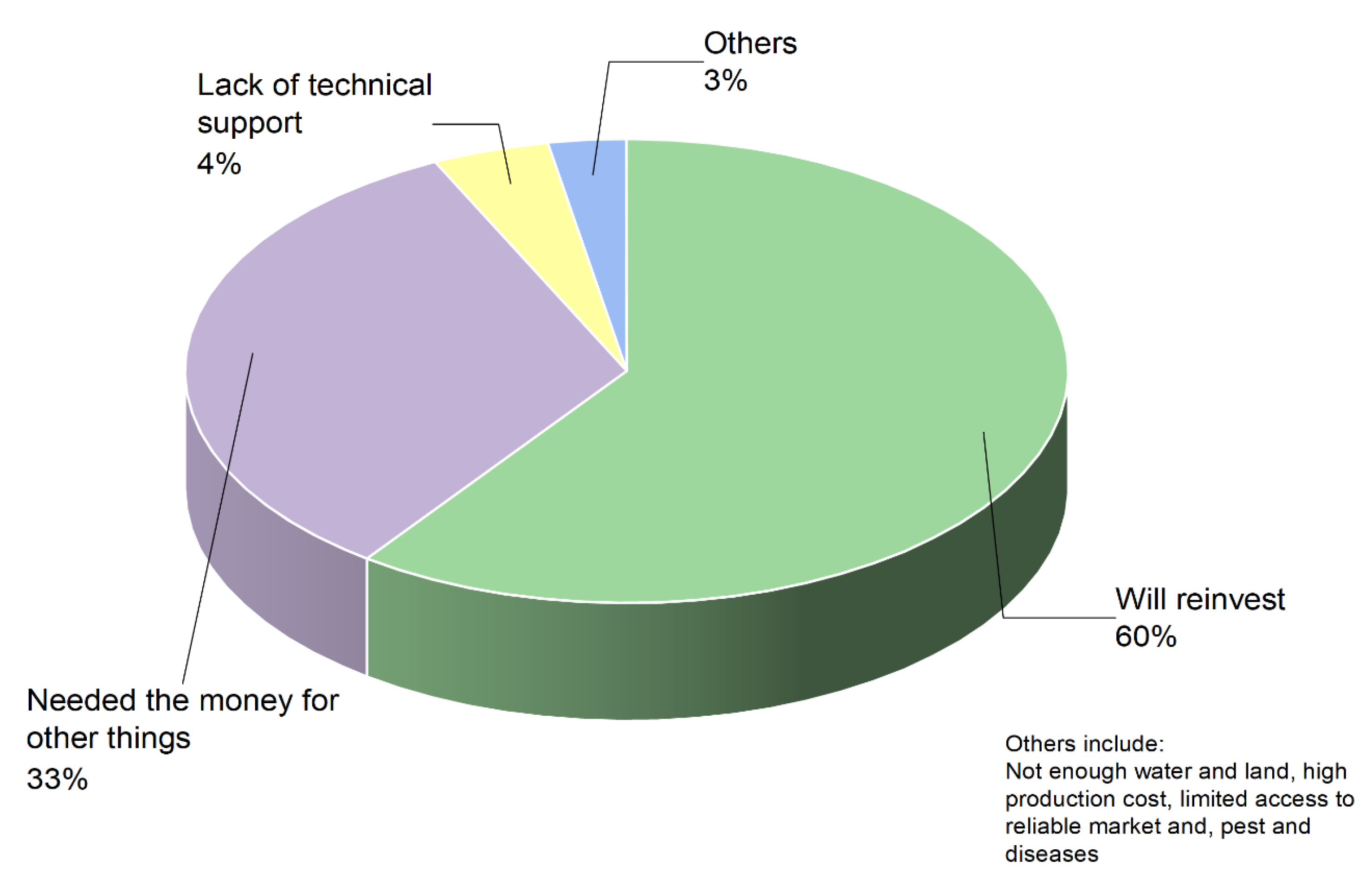
3.6. Key Factors Affecting Decision to Re-Invest

For the program’s viability and growth, it is important to examine the proportion of farmers who had re-invested income and the factors that have influenced their decisions not to reinvest. Importantly, sixty percent of MI farmers decided to reinvest in additional kits, with an increase in profit most frequently cited as the reason. The most common reason for not reinvesting (33%) was their need to use the income for other purposes, such as education, household assets, health care, or other urgent requirements. A small number (4%) of the respondents reported a lack of technical support for agriculture, while 3 percent mentioned a lack of access to water and land, high production costs, limited access to reliable markets, and pest and disease problems as reasons for not reinvesting their additional earnings (Figure 9).

3.7. The Impact of the Implementation of the MI Program on Poverty

Although the MI program led to increased income, it did not necessarily translate into poverty reduction as defined by the poverty indicators. There were several plausible reasons for this. Firstly, the implementation of MI technology impacted to a variable extent on different households, and the socio-economic position of the household before investing in MI kits played an important role in determining the impacts. As the main target group of the program were poor households, it was likely that MI improved the livelihoods of many farmers, but to similar levels as the control farmers, since a number within this group also adopted the technology once they became familiar with it.

Since the average length of time for participation in the program was 12 months, it was likely that positive outcomes would accrue over a longer period: thus the impact of the program needs to be reassessed some years later.

According to the findings of this study, MI interventions increased vegetable yields, and when combined with higher market prices for their commodities, farmers have improved their livelihoods. More than 60% (Figure 9) of smallholder farmers were willing to reinvest in purchasing additional drip irrigation kits to boost their production. Our results emphasize the relevance of markets as a major aspect of this intervention. However, it is not guaranteed that these farmers will continue to experience high yields throughout the year because the soil nutrient analysis was absent, and nutrient-deficient soils will not be able to offer similar high yields. Several studies from the region have highlighted the importance of soil quality and analysis [36,37,38]. As a result, NCA and other implementing partners should consider soil analysis as part of their MI-intervention to help mitigate risk.

4. Limitations

The results of this study must be understood considering several important limitations.

For the poverty analysis, the cross-sectional design of this evaluation represented a key limitation. Collecting data, at one point in time, did not allow for more than a snapshot of a particular group at that time point. Since income generated from the micro-investment in drip irrigation can be used for various purposes by the farmers, the translation of such income into poverty reduction might take time, and repeated surveys over time may help to provide a more accurate estimate of poverty reduction.

5. Conclusions

• The MI initiative using drip irrigation has the potential to improve the livelihoods of smallholder farmers by increasing their farm yield and income. However, the increased income can be used in different ways, including asset building, child education, and loan repayment, all of which contribute to improving the livelihoods of farming communities.
• MI as an intervention for income generation is more effective when combined with initiatives that build market links that assure reasonable product prices. Thus, stakeholders (such as NCA) should consider better market linkages to gain a good price for smallholders’ produce.
• Farm enterprises that generate a variety of products, including crops, vegetables, and livestock farming, become more sustainable and resilient to adverse climatic effects. Improved extension and market linkages for all farm activities, as well as the provision of drip irrigation kits, have the potential to increase farm profitability and, as a result, provide a way out of poverty for smallholders.
• Assessment of the impact of drip irrigation technology over several growth seasons will provide a more accurate estimate of its value in utilizing the most important resource for successful cropping, namely the world’s ever dwindling supply of fresh water.

References

1. Tusting, L.S.; Bisanzio, D.; Alabaster, G.; Cameron, E.; Cibulskis, R.; Davies, M.; Flaxman, S.; Gibson, H.S.; Knudsen, J.; Mbogo, C. Mapping changes in housing in sub-Saharan Africa from 2000 to 2015. Nature 2019, 568, 391–394. [Google Scholar] [CrossRef] [PubMed] [Green Version]
2. Lowder, S.K.; Skoet, J.; Raney, T. The number, size, and distribution of farms, smallholder farms, and family farms worldwide. World Dev. 2016, 87, 16–29. [Google Scholar] [CrossRef] [Green Version]
3. Maliki, M.A.; Pauline, N.M. Living and Responding to Climatic Stresses: Perspectives from Smallholder Farmers in Hanang’ District, Tanzania. Environ. Manag. 2022, 1–14. [Google Scholar] [CrossRef] [PubMed]
4. FAO. The United Republic of Tanzania Resilience Strategy 2019–2022; Food and Agriculture Organization of the United Nations: Rome, Italy, 2019; Available online: http://www.fao.org/3/ca4805en/ca4805en.pdf (accessed on 23 August 2021).
5. World Bank Group. Poverty & Equity Brief, Sub-Saharan Africa, Tanzania; World Bank Group: Washington, DC, USA, 2020; Available online: https://databankfiles.worldbank.org/data/download/poverty/33EF03BB-9722-4AE2-ABC7-AA2972D68AFE/Global_POVEQ_TZA.pdf (accessed on 31 August 2022).
6. IFPRI. International Food Policy Research Institute (IFPRI) and Datawheel. 2017. Available online: https://dataafrica.io/profile/united-republic-of-tanzania (accessed on 24 August 2022).
7. Biswas, S.; Akanda, A.; Rahman, M.; Hossain, M. Effect of drip irrigation and mulching on yield, water-use efficiency and economics of tomato. Plant Soil Environ. 2016, 61, 97–102. [Google Scholar]
8. Enfors, E.; Gordon, L. Analysing resilience in dryland agro-ecosystems: A case study of the Makanya catchment in Tanzania over the past 50 years. Land Degrad. Dev. 2007, 18, 680–696. [Google Scholar] [CrossRef]
9. Müller, C.; Cramer, W.; Hare, W.L.; Lotze-Campen, H. Climate change risks for African agriculture. Proc. Natl. Acad. Sci. USA 2011, 108, 4313–4315. [Google Scholar] [CrossRef] [PubMed] [Green Version]
10. Enfors, E.I.; Gordon, L.J. Dealing with drought: The challenge of using water system technologies to break dryland poverty traps. Glob. Environ. Chang. 2008, 18, 607–616. [Google Scholar] [CrossRef]
11. World Bank. The World Bank in Tanzania–Overview; World Bank Group: Washington, DC, USA, 2020; Available online: https://www.worldbank.org/en/country/tanzania/overview (accessed on 27 March 2022).
12. Zagst, L. Socio-Economic Survey CARE-MICCA Pilot Project in the United Republic of Tanzania: Final Report; United Nations Food and Agricultural Program: Rome, Italy, 2012; p. 178. [Google Scholar]
13. World Health Organization. The State of Food Security and Nutrition in the World 2020: Transforming Food Systems for Affordable Healthy Diets; Food & Agriculture Organization: Rome, Italy, 2020; Volume 2020. [Google Scholar]
14. Mkenda, B.K.; Van Campenhout, B. Estimating Transaction Costs in Tanzanian Supply Chains; International Growth Centre (IGC): London, UK, 2011; Available online: https://www.theigc.org/wp-content/uploads/2011/11/Mkenda-Van-Campenhout-2011-Working-Paper.pdf (accessed on 27 March 2022).
15. WFP. Food Consumption Analysis Calculation and Use of the Food Consumption Score in Food Security Analysis; World Food Programme: Rome, Italy, 2008; Available online: https://documents.wfp.org/stellent/groups/public/documents/manual_guide_proced/wfp197216.pdf (accessed on 22 August 2022).
16. FAO. The State of Food Security and Nutrition in the World; Transforming Food Systems for Affordable Healthy Diets; Food and Agriculture Organization of the United Nations: Rome, Italy, 2018; Available online: http://www.fao.org/3/i9553en/i9553en.pdf (accessed on 12 January 2022).
17. Herforth, A.; Bai, Y.; Venkat, A.; Mahrt, K.; Ebel, A.; Masters, W.A. Cost and Affordability of Healthy Diets Across and within Countries: Background Paper for the State of Food Security and Nutrition in the World 2020. FAO Agricultural Development Economics Technical Study No. 9; Food & Agriculture Organization: Rome, Italy, 2020; Volume 9. [Google Scholar]
18. Kubzansky, M.; Cooper, A.; Barbary, V. Promise and Progress: Market-Based Solutions to Poverty in Africa; Monitor Group: Cambridge, MA, USA, 2011. [Google Scholar]
19. Scheyvens, R. Development Fieldwork: A Practical Guide; Sage: New York, NY, USA, 2014. [Google Scholar]
20. Sharma, G. Pros and cons of different sampling techniques. Int. J. Appl. Res. 2017, 3, 749–752. [Google Scholar]
21. Malcolm, L. Farm Management analysis: A core discipline, simple sums, sophisticated thinking. Aust. Farm Bus. Manag. J. 2004, 1, 45–55. [Google Scholar]
22. Edwards, W.; Duffy, P.; Kay, R. Farm Management; McGraw-Hill Higher Education: New York, NY, USA, 2015. [Google Scholar]
23. GHI. Global Hunger Index (GHI). 2020. Available online: https://www.globalhungerindex.org/tanzania.html (accessed on 21 November 2021).
24. Oxford Poverty & Human Development Initiative (OPHI) & United Nations Development Program (UNDP). Global Multideimensional Poverty Index 2020: Chartering Pathways Out of Multidimensional Poverty: Achieving the SDGs; OPHI: Oxford, UK; UNDP: New York, NY, USA, 2020; Available online: http://hdr.undp.org/sites/default/files/2020_mpi_report_en.pdf (accessed on 2 December 2021).
25. UNDP. Human Development Report 2019: Beyond Income, Beyond Averages, Beyond Todays: Inequalities in Human Development in the 21st Century; United Nations Development Program: New York, NY, USA, 2019; Available online: http://hdr.undp.org/sites/default/files/hdr2019.pdf (accessed on 12 December 2021).
26. Kabeer, N. Resources, agency, achievements: Reflections on the measurement of women’s empowerment. Dev. Chang. 1999, 30, 435–464. [Google Scholar] [CrossRef]
27. Alkire, S.; Meinzen-Dick, R.; Peterman, A.; Quisumbing, A.; Seymour, G.; Vaz, A. The women’s empowerment in agriculture index. World Dev. 2013, 52, 71–91. [Google Scholar] [CrossRef] [Green Version]
28. Malapit, H.; Quisumbing, A.; Meinzen-Dick, R.; Seymour, G.; Martinez, E.M.; Heckert, J.; Rubin, D.; Vaz, A.; Yount, K.M.; Phase, G.A.A.P. Development of the project-level Women’s Empowerment in Agriculture Index (pro-WEAI). World Dev. 2019, 122, 675–692. [Google Scholar] [CrossRef] [PubMed]
29. Doss, C.; Kovarik, C.; Peterman, A.; Quisumbing, A.; Van Den Bold, M. Gender inequalities in ownership and control of land in Africa: Myth and reality. Agr. Econ.-Blackwell 2015, 46, 403–434. [Google Scholar] [CrossRef]
30. IndiKit. Women’s Autonomy Index. 2021. Available online: https://www.indikit.net/indicator/327-women-s-autonomy-index (accessed on 28 August 2022).
31. WFP. Meta Data for the Food Consumption Score (FCS) Indicator; World Food Programme: Rome, Italy, 2015; Available online: https://www.wfp.org/publications/meta-data-food-consumption-score-fcs-indicator (accessed on 27 March 2022).
32. Maxwell, D.; Caldwell, R. The Coping Strategies Index Field Methods Manual, 2nd ed.; World Food Programme: Rome, Italy, 2008; Available online: https://documents.wfp.org/stellent/groups/public/documents/manual_guide_proced/wfp211058.pdf (accessed on 27 March 2022).
33. Bilinsky, P.; Anne, S. Months of Adequate Household Food Provisioning (MAHFP) for Measurement of Household Food Access: Indicator Guide (v.4); USAID FHI 360/Food and Nutrition Technical Assistance: Washington, DC, USA, 2010; Available online: https://www.fantaproject.org/monitoring-and-evaluation/mahfp (accessed on 27 March 2022).
34. Ayars, J.; Fulton, A.; Taylor, B. Subsurface drip irrigation in California—Here to stay? Agric. Water Manag. 2015, 157, 39–47. [Google Scholar] [CrossRef]
35. Markelova, H.; Meinzen-Dick, R.; Hellin, J.; Dohrn, S. Collective action for smallholder market access. Food Policy 2009, 34, 1–7. [Google Scholar] [CrossRef] [Green Version]
36. Snapp, S.S. Soil nutrient status of smallholder farms in Malawi. Commun. Soil Sci. Plant Anal. 1998, 29, 2571–2588. [Google Scholar] [CrossRef]
37. Nyamasoka-Magonziwa, B.; Vanek, S.J.; Ojiem, J.O.; Fonte, S.J. A soil tool kit to evaluate soil properties and monitor soil health changes in smallholder farming contexts. Geoderma 2020, 376, 114539. [Google Scholar] [CrossRef]
38. Mowo, J.G.; Janssen, B.H.; Oenema, O.; German, L.A.; Mrema, J.P.; Shemdoe, R.S. Soil fertility evaluation and management by smallholder farmer communities in northern Tanzania. Agric. Ecosyst. Environ. 2006, 116, 47–59. [Google Scholar] [CrossRef]
Figure 1. Map of Tanzania: the study districts are highlighted in green.
Agriculture 12 01732 g001
Figure 2. Micro-investing (MI) and control farmers (%) producing crops and vegetables in all four study districts in Tanzania.
Agriculture 12 01732 g002
Figure 3. Enterprise comparison of MI farmers (a) and control farmers (b) growing Amaranthus and cabbage in the Hai district. Price, revenue, total variable cost (TVC), and gross margin (GM) amounts are presented in Tanzanian Shilling (TSh), where 1 USD = 2330 TSh and 1 TSh = 0.00043 USD. Yield is calculated as per bed per season. Standard error of mean is presented as error bars for each bar graph.
Agriculture 12 01732 g003
Figure 4. Enterprise comparison of MI farmers (a) and control farmers (b) growing Loshuu (Hai district) and Amaranthus (Kasulu district). Price, revenue, total variable cost (TVC), and gross margin (GM) amounts are presented in Tanzanian Shilling (TSh), where 1 USD = 2330 TSh and 1 TSh = 0.00043 USD. Yield is calculated as per bed per season. Standard error of mean is presented as error bars for each bar graph.
Agriculture 12 01732 g004
Figure 5. Enterprise comparison of MI farmers (a) and control farmers (b) growing cabbage and Chinese cabbage in the Kasulu district. Price, revenue, total variable cost (TVC), and gross margin (GM) amounts are presented in Tanzanian Shilling (TSh), where 1 USD = 2330 TSh and 1 TSh = 0.00043 USD. Yield is calculated as per bed per season. Standard error of mean is presented as error bars for each bar graph.
Agriculture 12 01732 g005
Figure 6. Enterprise comparison of MI farmers (a) and control farmers (b) growing tomatoes (Kasulu district) and Amaranthus (Kilosa district). Price, revenue, total variable cost (TVC), and gross margin (GM) amounts are presented in Tanzanian Shilling (TSh), where 1 USD = 2330 TSh and 1 TSh = 0.00043 USD. Yield is calculated as per bed per season. Standard error of mean is presented as error bars for each bar graph.
Agriculture 12 01732 g006
Figure 7. Enterprise comparison of MI farmers (a) and control farmers (b) growing Chinese cabbage and hot peppers in the Kilosa district. Price, revenue, total variable cost (TVC), and gross margin (GM) amounts are presented in Tanzanian Shilling (TSh), where 1 USD = 2330 TSh and 1 TSh = 0.00043 USD. Yield is calculated as per bed per season. Standard error of mean is presented as error bars for each bar graph.
Agriculture 12 01732 g007
Figure 8. Enterprise comparison of MI farmers (a) and control farmers (b) growing pawpaw in the Kilosa district. Price, revenue, total variable cost (TVC), and gross margin (GM) amounts are presented in Tanzanian Shilling (TSh), where 1 USD = 2330 TSh and 1 TSh = 0.00043 USD. Yield is calculated as per bed per season. Standard error of mean is presented as error bars for each bar graph.
Agriculture 12 01732 g008
Figure 9. A comparison of MI farmers who reinvested in the vegetable kits and most common reasons for not reinvesting in vegetable kits.
Agriculture 12 01732 g009