Defect Detection using Power Spectrum of Torsional Waves in Guided-Wave Inspection of Pipelines

Abstract

Ultrasonic Guided-wave (UGW) testing of pipelines allows long-range assessment of pipe integrity from a single point of inspection. This technology uses a number of arrays of transducers separated by a distance from each other to generate a single axisymmetric (torsional) wave mode. The location of anomalies in the pipe is determined by inspectors using the received signal. Guided-waves are multimodal and dispersive. In practical tests, nonaxisymmetric waves are also received due to the nonideal testing conditions, such as presence of variable transfer function of transducers. These waves are considered as the main source of noise in the guided-wave inspection of pipelines. In this paper, we propose a method to exploit the differences in the power spectrum of the torsional wave and flexural waves, in order to detect the torsional wave, leading to the defect location. The method is based on a sliding moving window, where in each iteration the signals are normalised and their power spectra are calculated. Each power spectrum is compared with the previously known spectrum of excitation sequence. Five binary conditions are defined; all of these need to be met in order for a window to be marked as defect signal. This method is validated using a synthesised test case generated by a Finite Element Model (FEM) as well as real test data gathered from laboratory trials. In laboratory trials, three different pipes with defects sizes of 4%, 3% and 2% cross-sectional area (CSA) material loss were evaluated. In order to find the optimum frequency, the varying excitation frequency of 30 to 50 kHz (in steps of 2 kHz) were used. The results demonstrate the capability of this algorithm in detecting torsional waves with low signal-to-noise ratio (SNR) without requiring any change in the excitation sequence. This can help inspectors by validating the frequency response of the received sequence and give more confidence in the detection of defects in guided-wave testing of pipelines.

1. Introduction

Pipelines are the main means of transferring oil and gas. They are usually installed in hostile locations and must be inspected to avoid failures that would be harmful to the environment. Ultrasonic guided-wave (UGW) enables long-range inspection of pipelines from one single test point. For example, the UGW technique in pulse-echo mode can enable inspections of up to 50 m (in normal testing conditions); hence, it is cost efficient in the inspection of large structures. The received signals are inspected in time-domain where inspectors spot anomalies in the data based on their local signal-to-noise ratio (SNR). In any region where the envelope of the signal has higher energy than the regional noise level, an anomaly is reported which can indicate a defect or a feature of the pipe [1,2,3]. UGWs are multimodal: for each excitation frequency, multiple wave modes are transmitted and received. In the inspection, the goal is to achieve a pure axisymmetric wave, but due to the imperfect testing conditions [4,5], nonaxisymmetric waves will also be received. This is the main source of the coherent noise in the inspection. To allow ease of inspection, many researchers have applied digital signal processing methods that use the differences in these wave modes to either detect the axisymmetric wave or filter the nonaxisymmetric waves to increase the SNR of the received anomalies. One of the widely used techniques in the signal processing of guided-waves is the work of Wilcox et al. [6], which uses previously calculated dispersion curves in order to compensate for the effect of dispersion for the wave mode of interest in a certain propagation distance. In 2013, Zeng et al. [7] used the basis of the dispersion compensation technique and introduced a novel method to design waveforms in order to precompensate for a certain propagation distance.

Pulse compression is another approach that has been previously investigated in the literature. Instead of exciting a narrowband sine wave sequence, pulse compression uses a known coded sequence and processes the received signal by applying match-filtering in order to detect the known sequence. One of the initial attempts of testing pulse compression in the guided-wave was done by Rodriguez et al. [8,9], where chirp sequences were excited using air-coupled piezoelectric transducer in order to generate Lamb waves in aluminum plates. Higher SNR and peak values for the signals of interests were achieved in the experiments; however, the effect of dispersion was not considered, and therefore a decrease in signal amplitude was expected. In 2010, they published another paper using the same system where the phase modulation based on Golay codes were used where the enhancement of 21 dB in SNR using a 16-bit Golay code was achieved compared to the conventional pulse transmission. Mehmet et al. [10,11], introduced an iterative dispersion compensation for removing the dispersion effect of guided-wave propagation. Most recently, Malo et al. [12] developed a two-dimensional compressed pulse analysis in order to enhance the achieved SNR of each wave mode. In the pulse compression approaches, the results are always a trade-off between the spatial resolution and SNR, as having a result with higher propagation energy and δ-like correlation means that the signal duration must be increased. Furthermore, the transfer function of the excitation system can affect the accuracy of the coded waveforms. These two factors indicate that the initial waveform design and the accuracy of inspection using this method depend on the testing conditions.

On the other hand, other approaches have also been reported in the literature where narrowband sine waves were used as excitation sequence. Kamran et al. investigated split-spectrum processing [13,14,15], where the time-domain signal is decomposed into multiple signals in different frequency bands, and then recombined in time-domain in order to remove the coherent noise. In their most recent work [15], it was reported that using the optimum filter parameters and polarity thresholding method for recombination, the SNR of defects with sizes as small as 2% cross-sectional area (CSA) could be improved significantly. Nonetheless, the technique depends on various parameters which can depend on the pipes’ characteristics. Another recently developed method is the spectral subtraction, investigated by Duan et al. [16]. In this method, the noise signature is calculated using a small section of the retrieved signal where no real pipe feature exists. Afterwards, this signal is subtracted from the total signal using a sliding window where a significant reduction of coherent noise level could be achieved. Nonetheless, achieving noise signature in the practical inspection of pipelines is difficult as the location of defects and even pipe features might be unknown.

Guided-waves are dispersive and multimodal [17]. Depending on the excitation frequency, multiple wave modes can be generated at the point of excitation. Guided-wave modes are categorised based on their displacement patterns (mode shapes) within the structure. Three main families of waves exist in pipes, which are longitudinal, torsional and flexural. Longitudinal and torsional waves are axisymmetric waves, while flexural waves are nonaxisymmetric. The popular nomenclature used for them are in the format of X (n,m), where X can be replaced by the letters L for longitudinal, T for torsional and F for flexural waves; n shows the harmonic variations of displacement and stress around the circumference and m represents the order of existence of the wave mode [18]. In general inspection, the practice is to generate a single pure axisymmetric wave which tends to ease the interpretation of results. However, variations in the transducers’ transfer function and their placement will cause the flexural waves to be received; furthermore, wave mode conversion also causes flexural waves to be received [5,17,18,19].

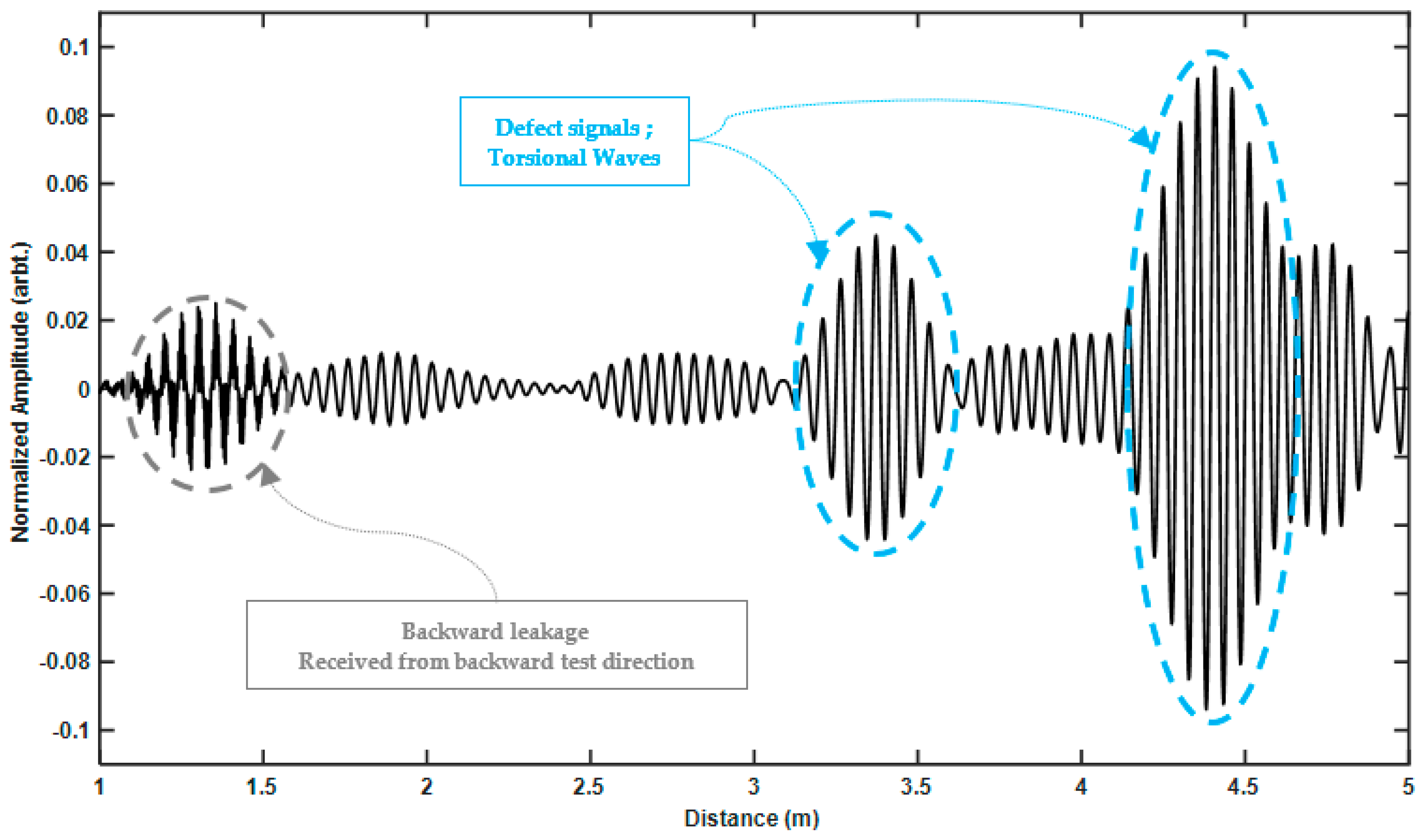
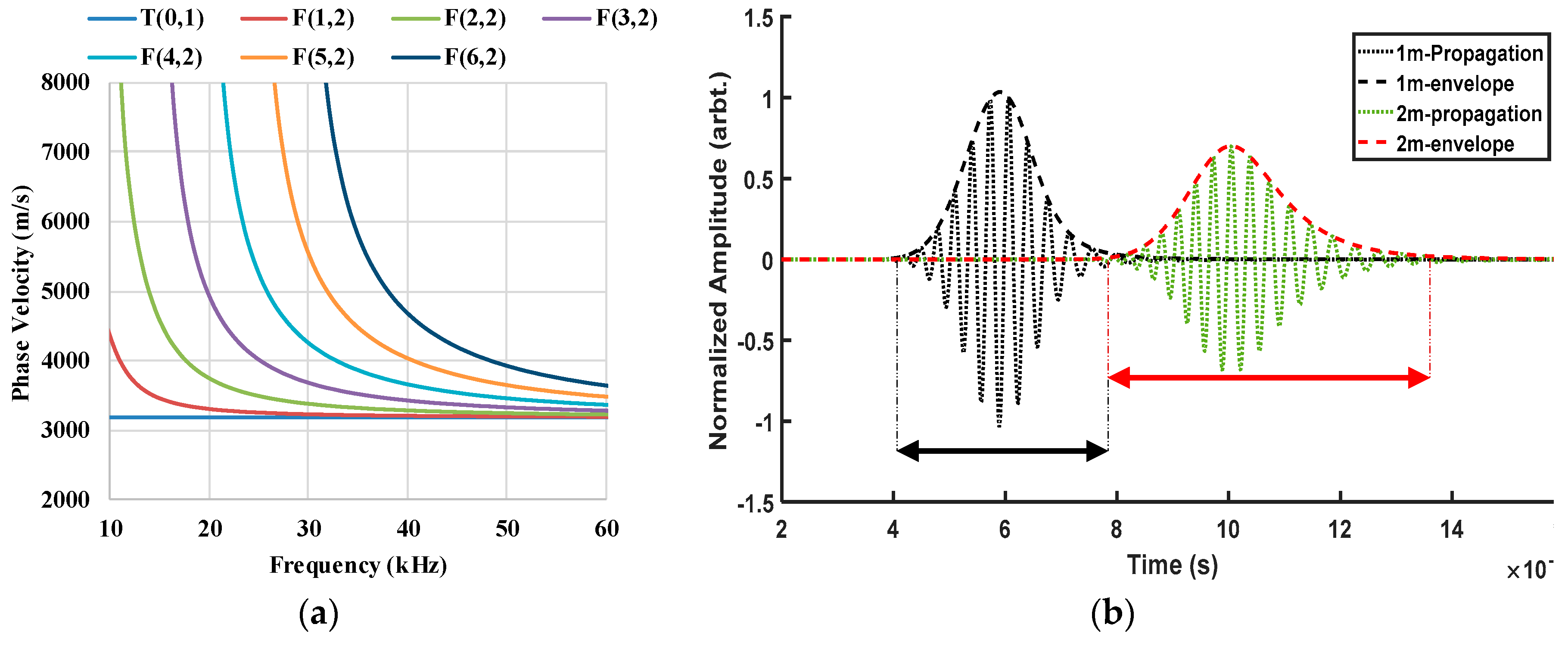
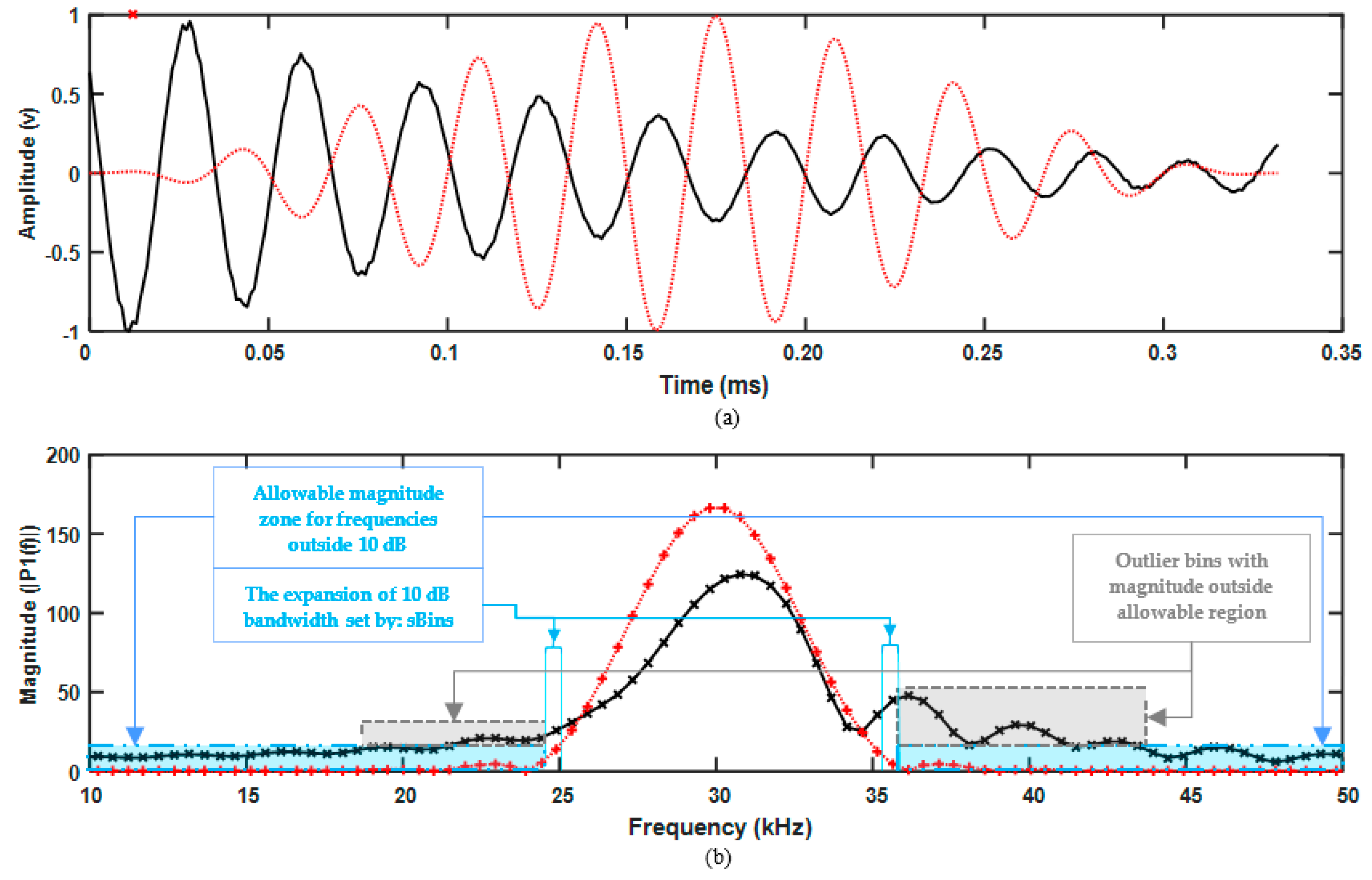
Dispersion causes the energy of a signal to spread out in space and time as it propagates [6]. Figure 1a shows an example of a dispersion curve calculated from 8-inch schedule 40 steel pipe using RAPID software [21]. Wilcox et al. introduced a method to use dispersion curves in order to both simulate [22] and remove [6] the effect of dispersion. Using the developed formula, an example of a dispersive wave is shown in Figure 1b, which is based on the dispersion curves of F (4,2). Unlike T (0,1), which is nondispersive across its whole frequency range [23], flexural waves are dispersive. Therefore, for ease of inspection, the torsional wave which is both axisymmetric and nondispersive is used.

The common concept in all the aforementioned signal processing methods is the usage of dispersion and multimodality of guided-waves in order to increase the SNR. Afterwards, the signals are inspected in time-domain to report on the location of anomalies. It has already been demonstrated in the literature that the spectral domain can be processed to remove the noise. Looking at the problem with another perspective, instead of noise removal, the spectral domain can also be used to detect the signal of interests (defect) automatically. The excitation sequence is not dispersive and axisymmetric; hence, no significant changes in the frequency response of the received signal should be inspected. Therefore, a sliding window is used where the power spectrum of each iteration is compared with the one achieved from the excitation sequence.

The primary motivation is to enable automated inspection of pipelines without the need for any inspectors. However, at this stage, the developed algorithm can be used as a tool, along with the conventional detection methods, to provide more certainty in interoperation of the results and reduce the number of outliers called due to the coherent noise. It is expected that experience of this algorithm will help develop automated inspection of pipelines. It should be noted that the experiments were performed with shorter pipe length. Nevertheless, the detectability of the defects is mostly dependent on the characteristics of the received signal. The algorithm can easily detect a perfect axisymmetric feature such as a weld in long-range. Nonetheless, for defects which are generally smaller in size and asymmetric, the hypothesis is that the feature can be detected if the characteristic of the torsional wave is still detectable in the received signal. It should also be noted, that as the inspection pipe length increases the energy of the flexural waves reduce due to their dispersion in time and the effect of attenuation on them. Therefore, false alarms using this method would be expected to be less in long-range inspections.

The paper is organised as follows. Section 2 explains the proposed method for detection of defects using torsional waves. Section 3 demonstrates the results of the method on both synthesised and real experimental data and, finally, Section 4 concludes the paper.

2. Methodology

In ultrasonic testing, the excitation sequence is known, and the inspectors generally look for signals with the same characteristics in the time domain to find their signals of interest, such as a defect in materials. In UGW, one of the common excitation sequences is a 10-cycle Hann windowed signal with different frequency, depending on the testing conditions. However, these signals are typically polluted by coherent noise which has similar temporal characteristics to those of defect signals.

It was mentioned beforehand that in the guided-wave, torsional waves are nondispersive and axisymmetric. The flexurals, which are the main source of coherent noise in the tests, are dispersive and nonaxisymmetric. In the power spectrum of an inspected pure torsional wave, the same characteristics of the spectrum of the excitation sequence must be observed; this is not the case for flexural waves due to their temporal and spatial variances. It should also be mentioned that asymmetric features (which is the case for most defects) generally reflect both torsional and flexural waves; where their corresponding reflection coefficients depends on the geometry of the feature. However, in this research, we focus our detection based on the detection of the torsional waves. The torsional wave is always reflected, and it is received symmetrically around the pipe circumference regardless of the features’ geometry or the wave propagation distance. Furthermore, in some cases, the flexural waves are considered as the coherent noise received due to mode conversion from the known features, leading to detection of false alarms in the tests. Hence, the focus is in detection of torsional wave in order to find the location of features.

In this paper, we propose a condition-based comparison of the power spectrum achieved from a moving window of the received signal and the spectrum of the normal excitation sequence. Keeping in mind that, since both flexural and torsional waves have the same main bandwidth (BW), correlating them would not be sufficient for distinguishing between them. Nonetheless, using this proposed method the torsional wave is identifiable. Another advantage of this method is that it is relying on the excitation sequence, which is known and set manually by the inspectors.

This algorithm consists of three main aspects: (1) initialisation, which initialises the excitation sequence and extract the required features for comparison; (2) main loop, that uses the advancing window and carries out the pre- and postprocessing of the conditions; and (3) conditions, which constitute the main processing, where the spectrum of each iteration is compared with the one achieved from excitation sequence.

Since the signals are processed digitally, and due to the limited resolution in this domain, in the following section all formulae and definitions are presented based on the sample number for the time-domain and bin number for the power spectrum. In doing so, better performance, in terms of speed is achieved as no unnecessary interpolation, is needed. The sampling frequency (Fs) used in the tests is 1 MHz which is a fairly common sampling frequency of guided-wave inspection devices.

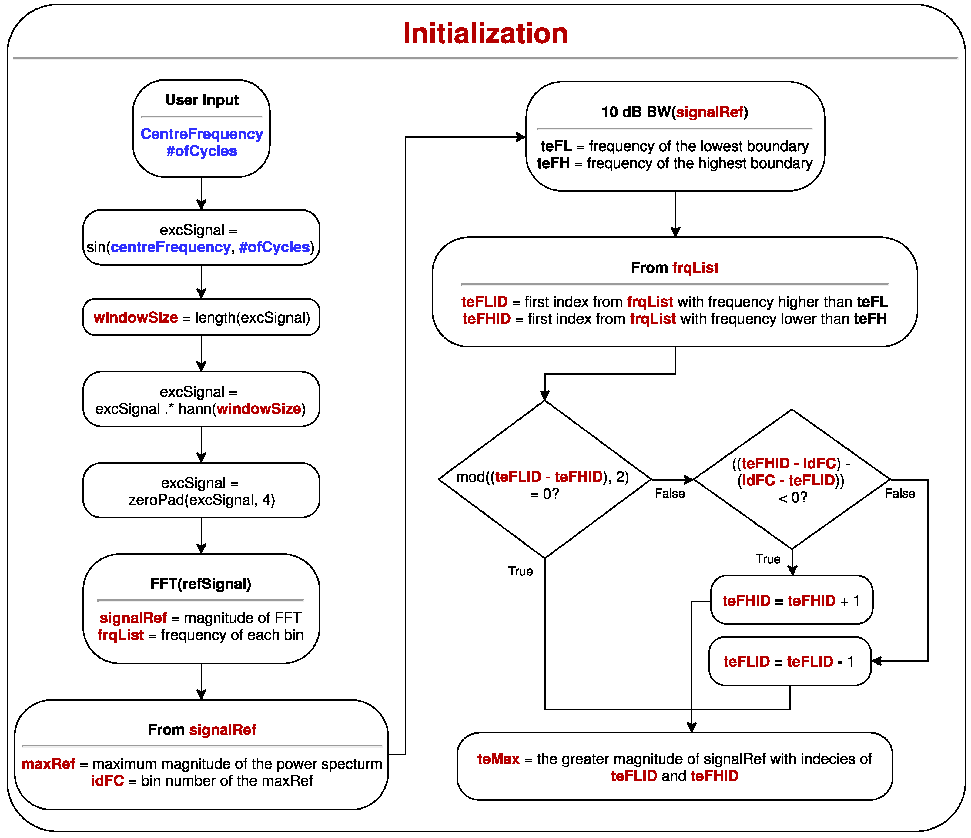
2.1. Initialisation

Initially, the excitation sequence is created where the inspector inputs the centre frequency and the number of cycles. Then, the “windowSize” is calculated based on the number of samples required for the excitation sequence. This sequence is already normalised by its maximum value. The normalisation bounds the signal amplitudes between 1 and −1 by dividing each sample by the maximum amplitude within the signal. Since 10 cycles are typically used for inspection, the duration of the excitation sequence is small; therefore, this signal is zero padded by a factor of 4 to achieve better resolution in the spectral density. Zero padding is the operation of adding extra zeroes to the end of the sequence in order to increase the resolution of the power spectrum [24]. The power spectrum is then evaluated by applying the fast Fourier transform [24], where the magnitudes of the spectrum are saved in “signalRef” and the corresponding frequency for each bin is saved in “frqList”.

The first extracted feature from the spectrum is the maximum magnitude and its corresponding bin number which are stored in “maxRef” and “idFC”, respectively. This should be the bin representing the centre frequency of excitation as set before by the inspector. Afterwards, the lowest and highest frequencies of the 10 dB BW of this spectrum are calculated. The bin numbers of the lowest and highest frequencies within this BW are saved in “teFLID” and “teFHID”. If the previously calculated “idFC” is not in the centre of this spectrum, these numbers are expanded away from the centre frequency so both the lower half and the upper half of the spectrum have the same amount of bin numbers. Then, the greater magnitude achieved from these (border) bins is stored in “teMax”. The flowchart of this function is shown in Figure 2 and a summary of the extracted variables are shown in

Table 1. Description of variables extracted from the Initialisation.

Variable Name	Description	Conditions
windowSize	Length of the moving window	-
signalRef	The power spectrum of the normalised excitation sequence	C2, C3, C4
frqList	List of the corresponding frequency for each bin number	C0
maxRef	Maximum magnitude achieved from signalRef	C4
idFC	Bin number of maxRef	C0
teFLID	Bin number of the lowest frequency within 10 dB bandwidth	C0, C1, C3
teFHID	Bin number of the highest frequency within 10 dB bandwidth	C0, C1, C3
teMax	The greater magnitude between teFLID and teFHID from signalRef	C3

. All values except “windowSize” are needed for the conditions function.

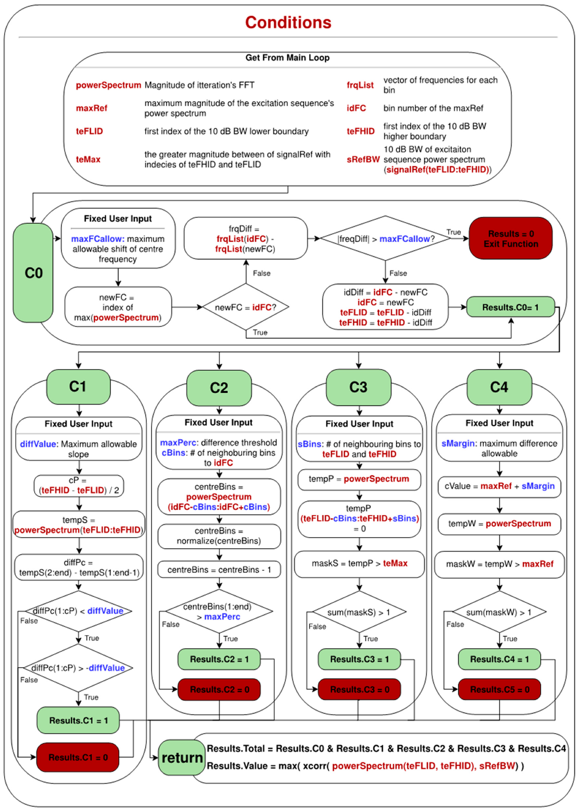
2.2. Conditions

In this function, all previously extracted characteristics are used in order to compare the spectrum of the moving window with the excitation sequence. The focus of this paper is on the similarity of the spectrum rather than the energy of the signals; thus, all signals are normalised before calculating the spectrum. Five conditions (features) exist in total. Since defect signals are affected by the flexural noises, it is expected that the received signals from smaller defects would not result in a perfectly matching spectrum. Hence, in each condition, safety variables are defined in order not to over-fit the conditions to the reference. These variables are set by the inspectors to provide a safety tolerance for detecting weak signals. It should be borne in mind that these tolerances have typically small values and can be fixed. Furthermore, they are set only once at the start of the algorithm and does not change iteratively.

2.2.1. Condition Zero (C0)

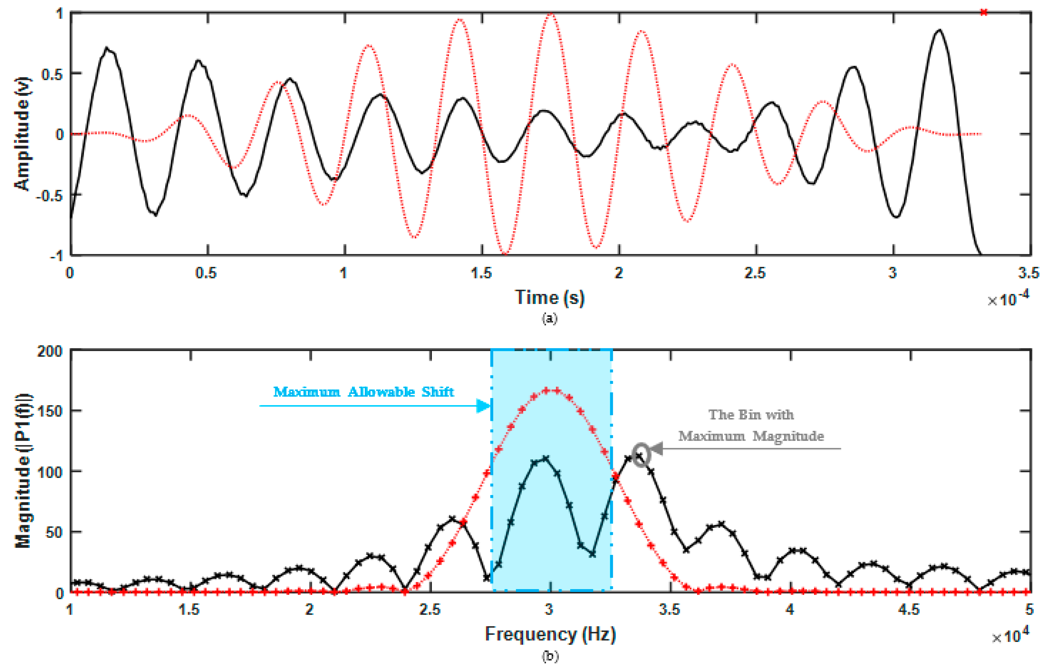
The centre frequency of the windowed spectrum must be near the centre frequency of the excitation sequence, defined by “idFC”. In case of small defect signals, where less energy is reflected, they are more affected by the coherent noise which will cause a slight shift in the centre frequency. Therefore, a slight shift in the frequency is acceptable which is defined by variable “maxFCallow”. If such a shift is detected, the corresponding bin numbers of “idFC”, “teFLID” and “teFHID”, which are required for the other conditions, will be shifted towards the new centre frequency of the spectrum. If this shift of centre frequency is more than maximum allowable shift, it means that the current iteration is significantly different to the excitation sequence and all other conditions will automatically fail. The maximum allowable shift, “maxFCAllow” is set to 3 kHz, which is a small margin in comparison to the total BW of the signal.

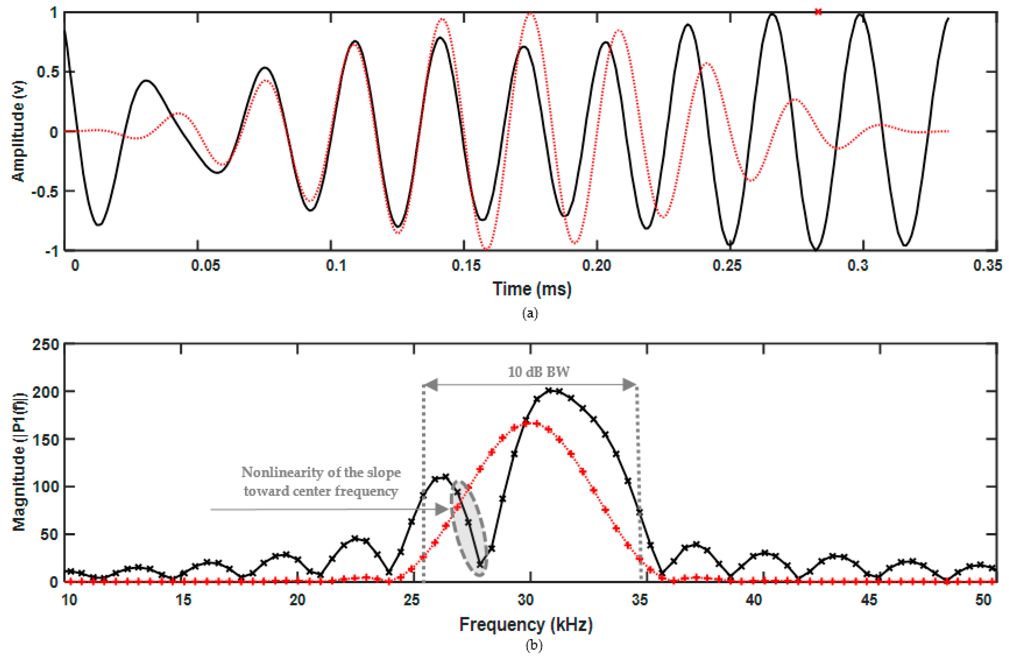
2.2.2. Condition One (C1)

In the Hann windowed sine waves, the lower half of the BW tends to increase in magnitude when moving towards the centre frequency then it starts to decrease. In this condition, it is checked that there is no discontinuity in this trend; in other words that no local maxima exist. In doing so, the 10 dB BW is of the main focus as the outside edges are typically affected by the flexural noises due to their lesser magnitudes. The reason for this is that in guided-wave inspection, (Hann) windowed, narrowband excitation sequences are used. Therefore, the main energy spread is within the main BW of the signal while a limited amount will be assigned to the borders of BW. The flexurals are dispersive, depending on their dispersion curves, their spectra tend to shift towards other frequencies, but the nondispersive torsional wave will not observe this change. Therefore, the energy of flexural waves will be stronger outside the main BW. Choosing 10 dB BW is a good compromise since more than 90% of the bins is covered using this value and only a few bins on the sides are neglected. Using the bin number of lowest frequency and the highest frequency in the 10 dB BW, “teFLID” and “teFHID”, it is checked whether the magnitude of each respective bin is increasing when moving toward the centre frequency. Nonetheless, a variable can also be defined as “diffVal” to allow small differences to be neglected. Currently, no tolerance is needed, and it is kept as zero.

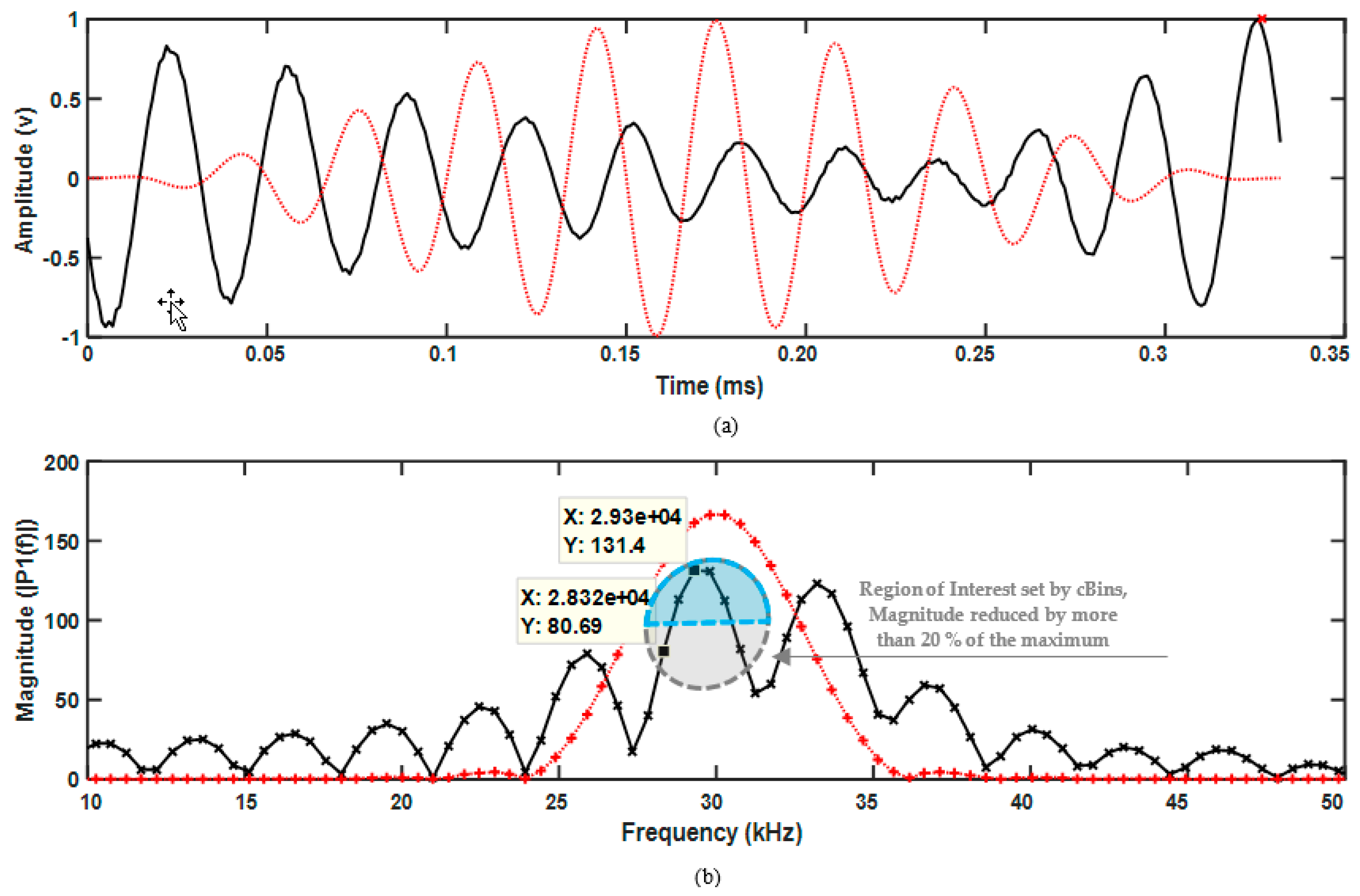
2.2.3. Condition Two (C2)

In the excitation sequence, the strongest magnitudes are detected in the region of the centre frequency. Since they have the strongest magnitude, they will be less affected by the noise in the region. In this condition, it is confirmed that the neighbourhood of the centre frequency has relatively the same magnitude. The number of neighbourhoods in each side of the centre frequency is defined by “cBins“, and the maximum allowable difference is defined based on a percentage of current iteration maximum magnitude defined by “maxPerc”. In this paper, the number of the neighbourhood is set as 2 and the maximum allowable difference is set as 20% of the maximum magnitude of each iteration.

2.2.4. Condition Three (C3)

The window size is set as the length of the excitation sequence. Due to this limited duration of the signal, in the iteration’s power spectrum, there should not be any magnitudes greater than the 10 dB BW boundary, “teMax”, of the excitation sequence other than the frequencies within these boundaries. Nonetheless, in the immediate bins next to the boundaries, “teFLID” and “teFHID”, the magnitudes are more affected by the coherent noise and can be greater than the “teMax”. Therefore, “sBins” is defined as the allowable number of immediate bins, which will be neglected during this comparison. This value is set to 1.

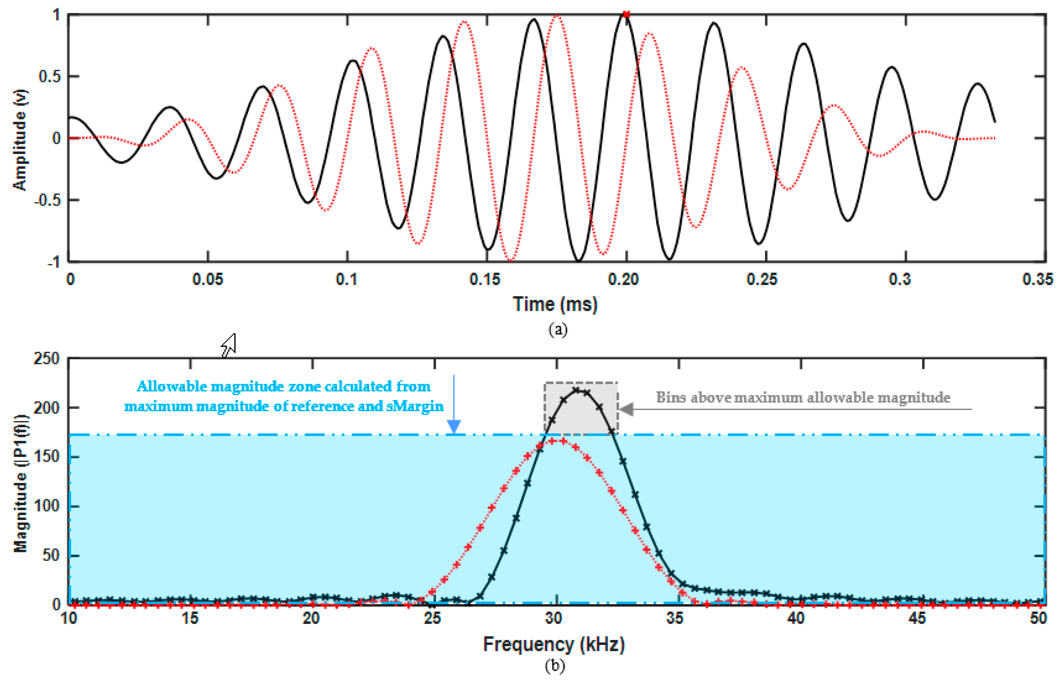
2.2.5. Condition Four (C4)

Each iteration window is normalised before its power spectrum is calculated. As the window size is limited to the excitation sequence, in the power spectrum of the iteration, a loss of magnitude can be expected due to the coherent noise in the signals. However, the maximum magnitude of the iteration cannot be greater than the one achieved from the excitation sequence, “maxRef”. Since normalisation is taking place, a small safety margin is defined as “sMargin”, to compensate for the small variances between the magnitudes defined. This value is set to 1, which is much less than the maximum magnitudes achieved from excitation sequences.

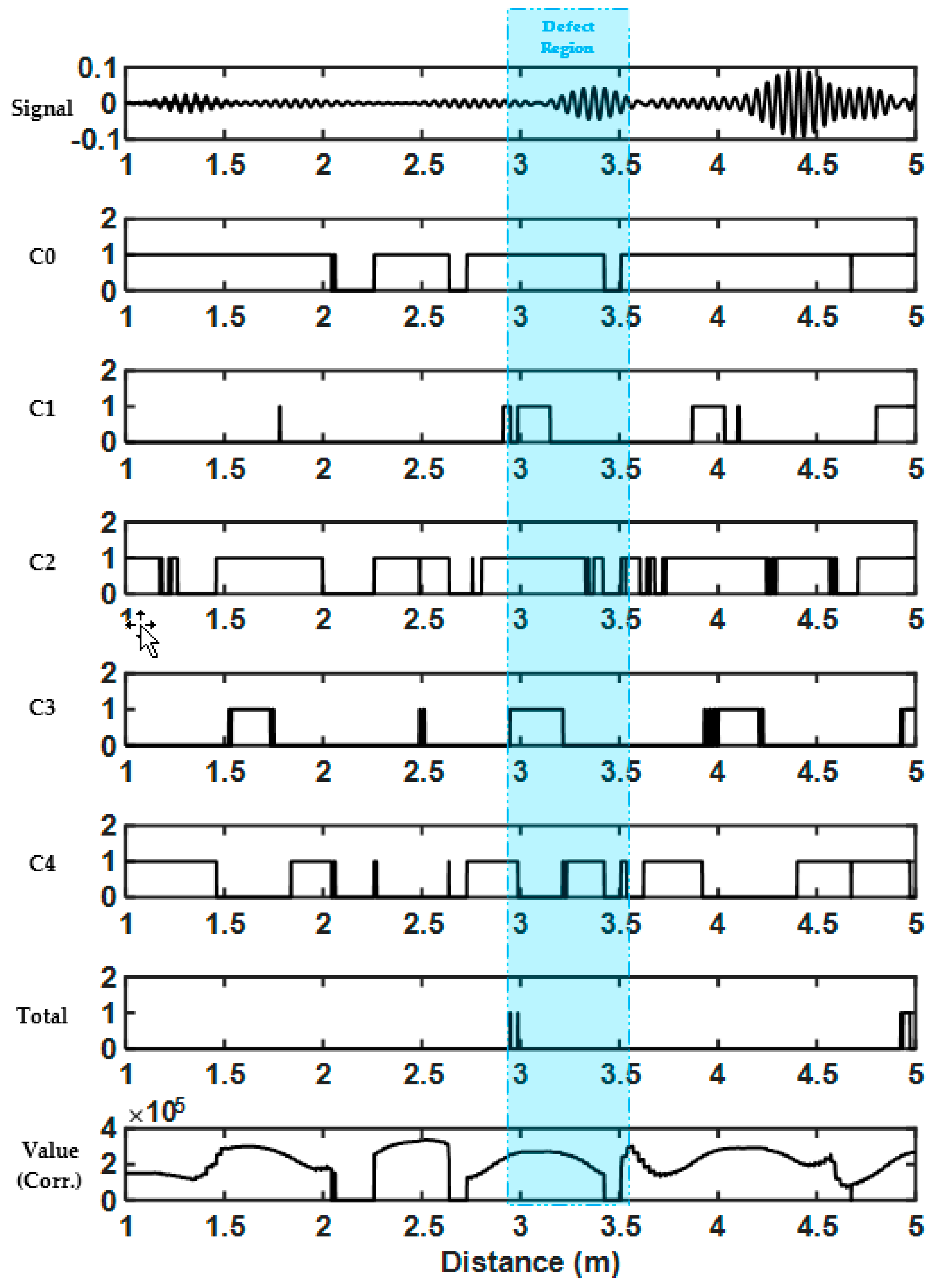
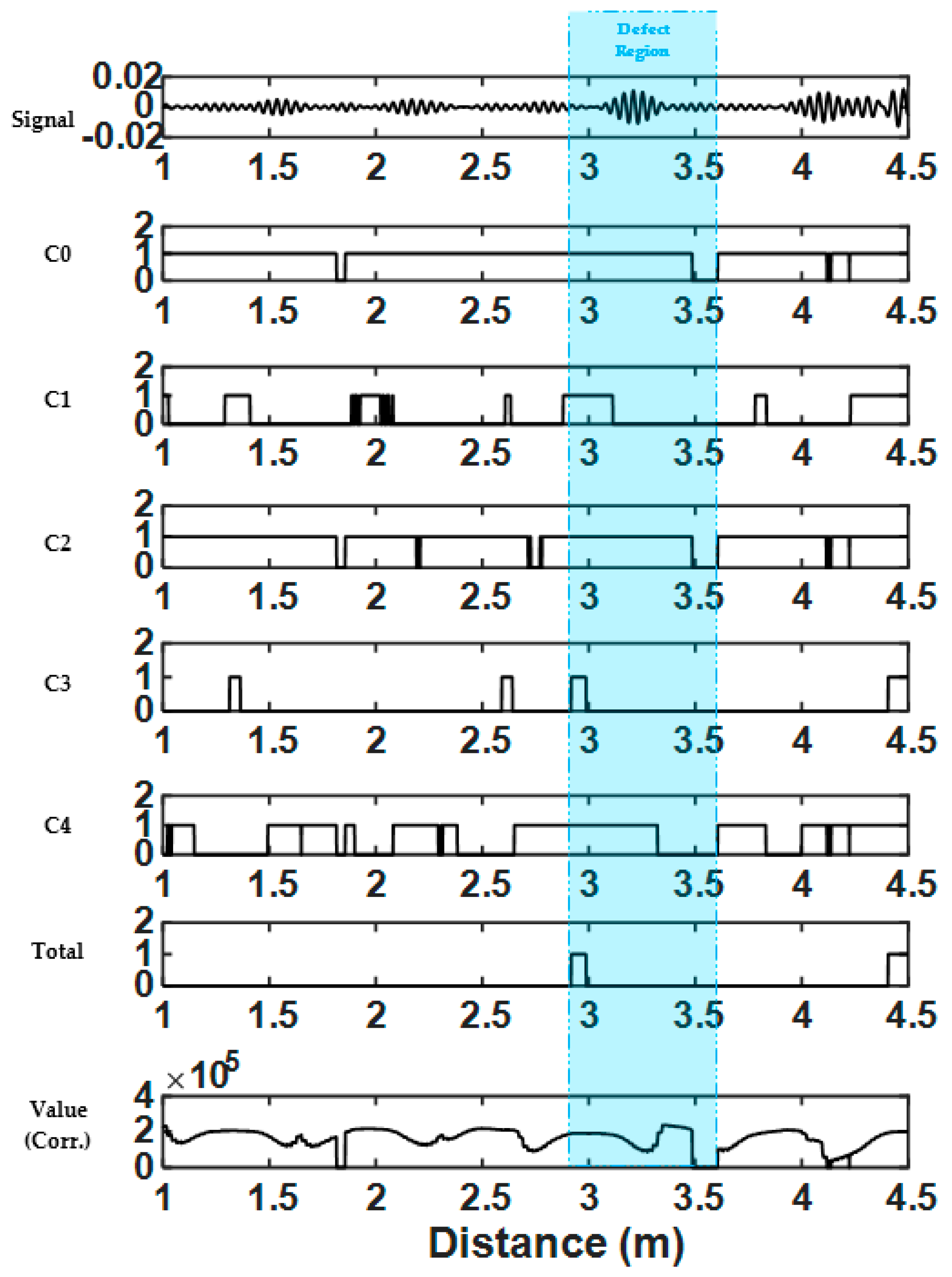
2.2.6. Final Results

Iterations are marked as the signal of interest (one) if all the aforementioned conditions are met and will be marked as noise (zero) if any of them are failed. Furthermore, the maximum correlation between the 10 dB BW of the power spectrum of the excitation sequence and current iteration is calculated. The cross-correlation of two sequences $\mathrm{x}\left[\mathrm{n}\right]$ and $\mathrm{y}\left[\mathrm{n}\right]$ is defined as [24]

$${\mathrm{r}}_{\mathrm{xy}}\left[\mathrm{l}\right]={{\displaystyle \sum }}_1^{\mathrm{N}}\mathrm{y}\left[\mathrm{n}+\mathrm{l}\right]\mathrm{x}\left[\mathrm{n}\right]$$

(1)

where $\mathrm{l}$ is the (time) shift (or) lag, $\mathrm{n}$ is the sample number of each sequence and $\mathrm{N}$ is the number of samples in the sequences. The correlation operation measures the degree to which two sequences are similar. As it can be seen in the formula, the output is given in a vector of time shifts. Therefore, by considering the maximum amplitude of ${\mathrm{r}}_{\mathrm{xy}}\left[\mathrm{l}\right]$, the maximum similarity between two sequences is measured. Nonetheless, since in C0, the peaks are shifted, no time shifting is required to achieve the maximum value and the results will become the summation of multiplication of each corresponding bin. Both the cross-correlation value and the binary condition results (“Total”) will be returned to the main loop where the final “detection” results will be generated. The flowchart of this function is shown in Figure 3.

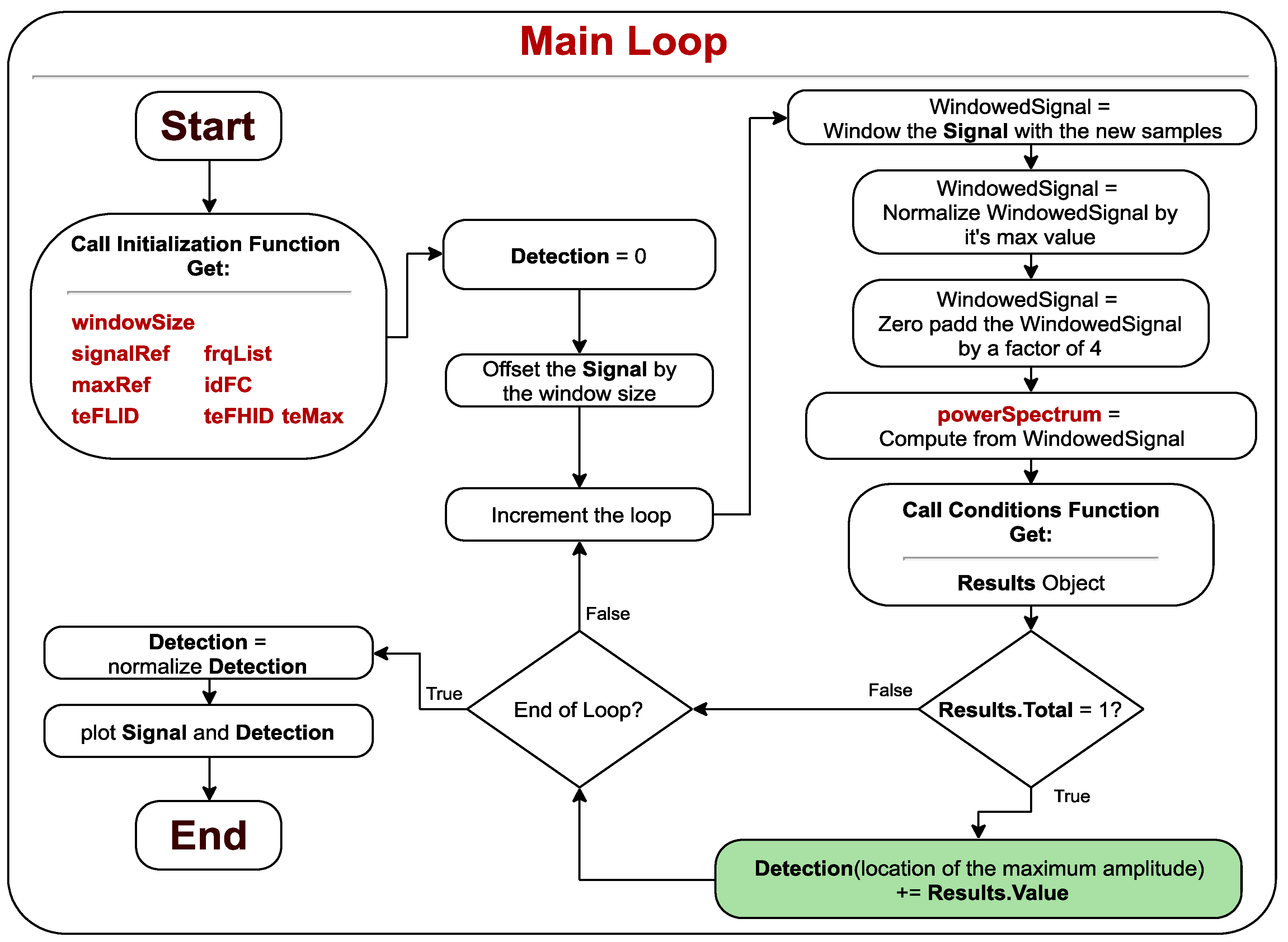
2.3. Main Loop

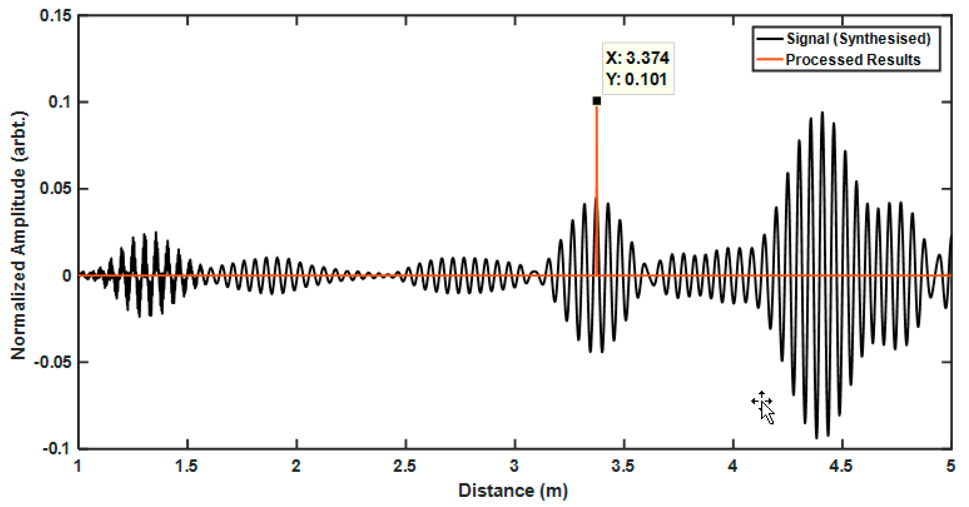
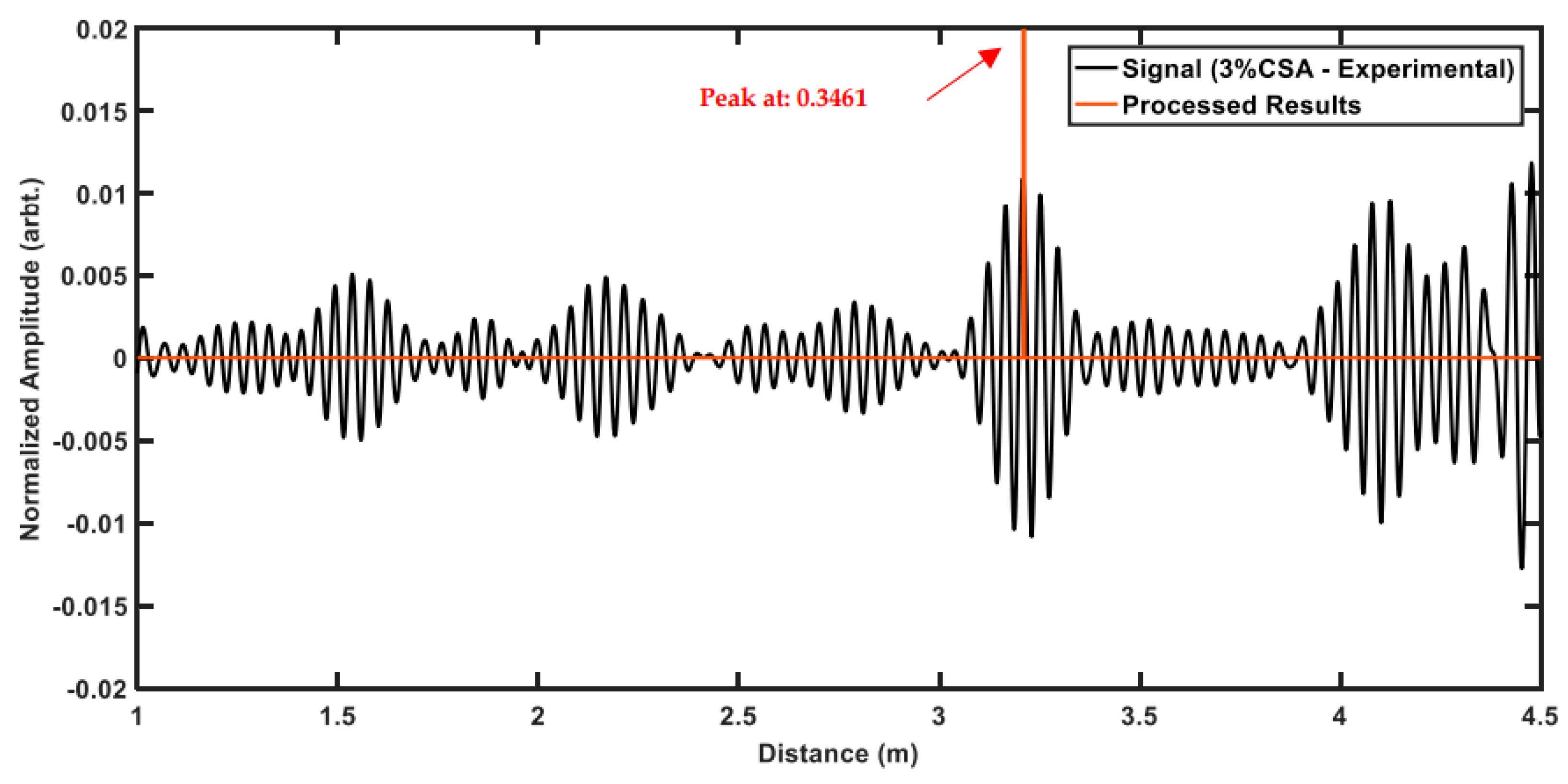
The initialisation is done before the main loop in order to extract the required features. Afterwards, the start of the iteration is delayed by the length of the window size. In practice, it means that the system can be linear and time invariant, and can be implemented in real-time as it only requires past samples of the signals. In each iteration, a temporary signal, “WindowedSignal”, is created which holds the past samples of the signals with the same length as the excitation sequence. Since the power spectra are needed to be compared, the signals are first normalised and zero padded by a factor of 4. The power spectrum of this windowed signal is calculated and passed to the conditions function. After processing, the “Results” object is returned where it contains the detection variable “Total” and the correlation value of the spectrums as “Value”. If the signal of interest is detected, e.g., “Total” is equal to one, then the current iteration represents a similar power spectrum to the one of excitation sequence.

One approach would be to mark the current iteration number as one which would mean that the current iteration is representing the signal of interest; however, this is not the best representation as the current iteration might not be the best representative of the windowed signal characteristics. In this paper, the index of the maximum amplitude in each windowed signal is detected. This index appears to be a better representation since the region with more energy has a stronger influence on the power spectrum. Since the excitation sequence is Hann windowed, the centre of the signal will hold the highest amount of signals’ energy. This as in this location, the concentration of signal energy is higher, stronger flexural features are required to disturb reduce/change the characteristics of this region. Therefore, the centre instead of adding the correlation value to the sides of the window (current iteration number), the value is cumulatively added to the location of the highest amplitude within the window, which represents the centre of the Hann windowed sequence in a torsional wave. This value is stored in “detection” vector. Therefore, the correlation value is added to the location where the signal represents the strongest amplitude in the “detection” vector. The reason why they are added rather than replaced is that since it is an iterative process, different windows can have the same index as the maximum; by doing a cumulative sum for each index, the certainty in defect detection is increased and the amplitudes assigned for the outliers and noises are decreased. The main loop finishes when the end of the signal is reached, at which point the “detection” vector is normalised and is plotted against the original signal to show the defect locations and their normalised correlation values. The flow chart of this function is shown in Figure 4.

3. Results

This method was initially developed on the FEM test case. As explained previously, the FEM model considers both spatial and temporal characteristics of guided-waves in order to simulate a coloured noise with similar characteristics of the noise in the real inspection. For a better understanding of the methodology, each condition is firstly explained using this FEM signal. To validate this method, the results on experimental pipes are shown. SNRs reported in this section as follows

$$\mathrm{SNR}=20\ast \log 10\left(\frac{\sqrt{\frac{1}{\mathrm{N}}{{\displaystyle \sum }}_1^{\mathrm{N}}\mathrm{Signal}\left[\mathrm{n}\right]}}{\sqrt{\frac{1}{\mathrm{M}}{{\displaystyle \sum }}_1^{\mathrm{M}}\mathrm{Noise}\left[\mathrm{m}\right]}}\right)$$

(2)

where “Signal” is considered as the samples where the defect (torsional wave) is expected to be received and every other sample is considered as Noise. In all tests, the excitation sequences are of 10-cycle Hann windowed sine waves, which are commonly used in the field inspections.

3.1. FEM Test Case

The generated signal in the FEM test case has the excitation frequency of 30 kHz, as shown in Figure 5. This setup of the model was previously explained in [25]. Modelling of guided-wave signals using FEM have been widely used and validated in the literature [2,26,27,28]. However, the major difference in this model is that the excitation sequences have variable transfer functions and fewer reception points are used; this tends to add flexural noise in data. In this figure, for better illustration of the signal, the received signal from (forward) the pipe end and the starting dead zone are removed. The defect signal is expected to be received at 3–3.5 m. Since highly variable transfer functions have been used, the backward cancellation algorithm is not able to cancel the backward going signal perfectly. This reversed wave reflected from the pipe end is received at 1–1.5 m. Due to this backward leakage, another signal of interest, which is a torsional wave, is expected to be received at approximately 4–4.5 m. This signal is generated when the echo of the backward leakage and the defect signal (in the forward testing direction) is received at the test tool. All other regions are the noise caused by the flexural waves.

3.1.1. Condition Zero

The starting condition is that the maximum magnitude of each iteration’s power spectrum must belong to the approximate region of the centre frequency. This approximation is set by the inspector (“maxFCAllow”). It is a necessary factor for the detection of smaller defects since the spectrum will be more affected by the flexural waves, which leads to a shift in centre frequency. An example of an outlier based on this condition is shown in Figure 6, where the blue box shows an example allowable region for frequency shift, and the grey circle shows the bin with the maximum magnitude in this iteration. Since it is outside the allowable region, the outcome of this condition will be zero, which will automatically force all other conditions to zero. The used value for the maximum allowable shift is 3 kHz which is a small margin in comparison to the overall BW of the excitation sequence. In the case of FEM signal, since the flexural wave does not affect the defect significantly, similar results can be achieved even when this value is set to zero.

3.1.2. Condition One

In simple terms, the magnitudes of each bin in the 10 dB BW of the iterations’ spectra must increase when moving toward the centre frequency. Due to dispersive nature and multimodality of guided-waves, this condition is not true for many iterations as a combination of waves will be received with different centre frequencies. Nonetheless, this condition must be true in the case of the torsional wave as it will have the same characteristic of the excitation waveform. Figure 7 shows an example of an outlier detected based on this condition. As can be seen, in the region between 26.5 to 27.5 kHz, the magnitude of three frequencies are actually decreasing, and a local minima is created. This suggests that the iteration is actually two separate wave modes with two different centre frequencies.

In this condition, in order to avoid marginal errors due to the limited number of samples in the window, a safety variable (“diffValue”), so the condition holds true if a slight decrease in the magnitude of each consecutive bin, is detected. In these tests, this value is kept at zero which means strictly positive increase of the magnitudes must be observed when moving toward centre frequency. The reason is, in case of guided-waves testing, if the flexural waves are strong enough that the frequency characteristics of the excitation waveform are changed, the signal must not be marked as a defect; since, in effect, the iteration is representing a strong existnace of a flexural wave.

3.1.3. Condition Two

The strongest magnitudes are in the neighbourhood area of the centre frequency; hence, they are less affected by the flexural waves. This condition verifies that the magnitudes from centre frequencies are not below a certain limit. Figure 8 shows an example of an outlier detected from this condition. Two limits must be set for this condition: (1) the number of neighbouring in “cBins” and (2) the percentage of allowable drop with regards to the maximum magnitude detected in the iteration (“maxPerc”). In these tests, “cBins” is set as two (of each side of centre frequency), which means a total of four bins is checked and thus limits this validation to the main central bins of the spectrum. In the reference signal, it can be seen that at the border of this region, an approximate 10% drop is observed. Since in practical testing, the magnitudes will be more affected by the flexural waves and testing condition, the allowable drop is set to 20% of the maximum magnitude of each iteration.

3.1.4. Condition Three

In the third condition, the magnitudes of frequencies outside the 10 dB BW of the excitation sequence are checked. Since the window size is limited to the length of the excitation sequence, no other strong peaks in other frequencies should be detected. This can be verified by confirming that no other magnitudes are above the lowest magnitude within 10 dB BW. Figure 9 shows an example for an outlier detected using this condition. The blue boxes illustrate the expected regions while the grey boxes illustrate the bins with higher magnitudes than the thresholds. It should be noted that this threshold is defined by the reference signal rather than the excitation sequence. Since the boundaries are affected more by flexural waves, a safe margin can be provided by expanding the bins away from the centre frequency (“sBins”). In these tests, this value is defined as one, which means only one bin is neglected from each side of the spectrum and all other bins must have magnitudes less than the minimum magnitude detected in the 10 dB BW.

3.1.5. Condition Four

In this condition, it is verified that the magnitude achieved in the power spectrum of iteration is not more than the reference. The reference signal is in the perfect form of the excitation when it is normalised and not affected by any noise, while any the windowed iterations are subject to noise; hence, the maximum magnitude of the iteration cannot be more than the reference. Nonetheless, due to the finite resolution of the windows, a safety value is defined as “sMargin” to allow small differences between the two to be neglected.

Keeping in mind that in the case of FEM signal, since source points were not placed linearly and variable transfer functions were used, the characteristics of the generated signals can be different. This is clearly illustrated in Figure 10, where the received has more than 10 cycles; hence, the maximum magnitude in the power spectrum of the iteration would be increased. The shown windowed signal is approximately located around the 4-metre region (second torsional wave), where the results of impact from backward leakage and the front defect are received from the forward direction. As can be seen, the condition will not hold in this case; however, when setting the threshold as 10% of the maximum magnitude (15) the result of the first detection is increased and this wave will also be detected. Changing this value to 15% increases the detection amplitude of the second signal and the pipe end even more, but the first defect signal remains constant. At 20%, the maximum values are achieved (while the overall detection result of the defect becomes less due to the increment of the associated value to the pipe end), and anything above does not change the generated results. Nonetheless, for the purpose of experimental tests, this value is only set as one which is less even than 1% of the maximum magnitude of the reference. This ensures that only calculation errors due to the limitation of the window size are neglected.

3.1.6. Results Total

The correlation results of the reference and the iteration’s power spectrum is added to the location of maximum voltage in each window. Furthermore, as the correlation result is typically a large number, the final result is normalised by the maximum value, which is typically the pipe end. This is illustrated in Figure 11 where it can be seen that the value of 0.1 is associated exactly to the centre of the defect signal. As illustrated, knowing only the excitation waveform, the approximate location of the defect is clearly detectable using this method.

The binary detection results of each condition for each iteration, as well as the total results, is demonstrated in Figure 12. In this figure, it is clearly demonstrated outliers exist in the results of each individual condition, but by combining all of them, only the iterations associated with the defect and pipe end are being detected. Furthermore, high correlation results are achieved from all iterations, irrespective of it being noise or defect; which is the main reason why doing a cross-correlation is not enough for detecting the defect location in the case of guided-wave testing. However, even with the existence of the coloured-noise, by checking the mentioned condition, the detection becomes possible.

In the same format, Figure 13 and Figure 14 show the results achieved from the 3% CSA defect from the experimental results. The same aforementioned conclusions can be drawn with regard to Figure 13. However, it can be seen that in the experimental results since the transfer functions are more linear, the outcome of condition 4 (C4) is true in most iterations. The results are shown in Figure 14, where the defect location is clearly marked using this algorithm. In overall, conditions one and three are the most effective ones which filter out most of the outliers from the tests.

These five conditions have not been optimised. Nevertheless, they were all designed based on the physical phenomena of guided-waves propagation within pipes. As can be seen in both the results of FEA and experimental tests, only in C3 and C4 could the defects be detected. However, having more relevant conditions, especially for practical inspection of pipes, may increase the certainty of the generated results. Nonetheless, the conditions are not necessarily required to be in the same Fourier Domain as stated in this algorithm, and the technique can be combined with other approaches, such as Wiener filtering, in order to improve its performance.

3.2. Experimental Results

A Teletest MK4 device [29], manufactured by Teletest branch of Eddify technology family in Cambridge (UK), was used in order to inspect an eight-inch schedule 40 steel pipe with a total length of six metres. The test tool included three rings of 24 linearly spaced thickness-shear (d15) transducers with 30-mm spacing, which are located 1.5 m away from the back end of the pipe. The device is capable of operating in pulse-echo mode with the operating frequency of 20 to 100 kHz, and maximum sampling frequency of 1 MHz. On the reception side, the individual sections received from each transducer is postprocessed in order to reduce the effect of echoes received from backward testing direction and flexural waves [5,17,30]. The schematic of the signal reception routes with this setup is shown in Figure 15.

The algorithm was assessed using data gathered from real pipes with three different defect size of 2%, 3% and 4% CSA. The defects were introduced using a saw-cut by thinning the wall thickness of the pipe’s circumference. The schematics of the defects and their approximate sizes are shown respectively in Figure 16 and

Table 2. Defect specifications.

CSA (%)	Flaw Depth (mm)	Cord Length (mm)	Arc Length (mm)
2	3.1	51.75	52.24
3	4.1	59.37	60.12
4	5	65.43	66.48

.

Depending on the system specification and test specimen, the maximum excitation power achieved by using frequencies in the range of 34 to 42 kHz. As can be seen in Figure 1a, most of the created flexurals from conversion of torsional wave is highly dispersive in the lower frequency region. Since dispersion affects the power spectrum of the received signal, it is expected that this algorithm works better with lower frequencies. However, the final choice of excitation frequency is a trade-off between the capability of the system to excite the required waveform and having highly dispersive flexural waves. Furthermore, it should be noted that the reflected wave amplitude at different frequencies is generally dependent on the flaw geometry, and this could effect the detection capability at different frequencies. In order to illustrate this dependency, 10 different frequencies have been used varying from 30 to 50 kHz with steps of 2 kHz. The achieved SNR from each signal of experimental tests are demonstrated in Figure 17 and

Table 3. Achieved SNR from defect signal in each test case (in dB).

CSA (%)	Frequency (kHz)
	30	32	34	36	38	40	42	44	46	48	50
4	7.13	8.84	11.12	12.15	13.13	13.76	13.23	11.73	9.50	6.84	3.50
3	4.29	5.97	8.15	8.62	9.08	9.51	9.00	7.60	5.43	2.82	−0.51
2	1.46	2.67	3.15	2.29	2.00	2.74	3.09	2.67	0.89	−1.43	−4.44

. As can be seen, 40 kHz achieved the best SNR in the tests; with a neglectable difference in the case of 2% CSA defect signal in comparison to other frequency (34 and 42 kHz). Nonetheless, all these defects are either close to the coherent noise level, which are generated by the unwanted flexural waves or are buried within it. Therefore, detecting these defects using normal inspection procedures without calling any outliers are challenging.

Figure 18 shows the processed results from each of these test cases where (a) shows the amplitude of detection and (b) shows the amplitude of outlier in the test. Outliers in these tests are considered as any detection corresponding to regions where the signal from neither defect or pipe features is expected to be received. In this figure, each line represents a defect with different CSA size and the value zero represents no detection. Furthermore, it can be seen that the algorithm works best in frequency range of 34–42 kHz. With these frequencies, defects with sizes above 3% can be detected with minor or no outliers existing in the results. In lower frequencies, although the amplitude of outliers is smaller than most test cases, defects with sizes smaller than 4% CSA cannot be detected. On the other hand, frequencies above 42 kHz generally result in the detection of outliers with higher amplitudes, where when using 48 and 50 kHz, no defect can be detected. The main reason is the transfer function of the system, where it is not capable of generating the expected power spectrum for the excitation waveform. As an example, consider the received signal from 50 kHz test case on 4% CSA pipe, is shown in Figure 19. The pipe end signal is a pure reflection of the excitation sequence where limited changes should be observed due to the coherent noise. The retrieved signal from the pipe end observes a 5 kHz shift in centre frequency. Furthermore, the generated sequence can also have a greater number of cycles which will result in higher maximum energy in an iteration’s power spectrum in comparison to the reference. Therefore, because of these significant changes which are caused by generation of the sequences, it is not recommended to use higher than 42 kHz excitation frequencies with this algorithm.

The only frequencies capable of detecting 2% CSA defect are 34, 36 and 40 kHz. With regards to Figure 20, which demonstrates the defect to outlier detection ratio, the detection amplitude achieved from defect from 34 and 40 kHz is higher by a factor of 1.5 and 2.38 than the outliers’, while, in the case of 36 kHz, this factor is only 0.36 which means the amplitude for defect detection is smaller. Nonetheless, for defects with higher CSA size, the detected defect to outlier amplitude ratio from tested frequencies in the range of 34 to 42 kHz is almost always higher than a factor of 2. This suggests that by setting an amplitude threshold, defects above 3% CSA size can be detected without any outliers. This threshold is shown in Figure 18 by the red dotted line which in this case is set as 0.2. It should also be borne in mind that doing so, would remove the detection of 2% CSA defect, especially in the case of 40 kHz since even though the values are smaller than this threshold, but the amplitude of defect detection (0.19) is approximately twice than those of outlier (0.08). The only two frequencies which do not detect any outliers in any of the tests are 30 and 38 kHz. Nonetheless, using 38 kHz, 2% CSA defect and using 30 KHz, both 2% and 3% CSA defects are not detected.

4. Conclusions

In this paper, a novel method is proposed to detect the location of defects using the known excitation power spectra of the torsional waves in guided-wave inspection of pipelines. For doing so, as opposed to traditional inspection using time-domain signal, the spectral domain of the signal is compared with the characteristics of the known excitation sequence. The method works by applying a moving window to the received signal from the inspection, where in each iteration the signal is normalised and its corresponding power spectrum is generated. Since both defect signal and noise are within the same frequency band, by only measuring the correlation between reference and iterations power spectrum, the defect signal will not be distinguishable. Therefore, before measuring the correlation, a total of five conditions were checked to verify that a similar power spectrum to the reference was achieved:

• Centre frequency shift must be small.
• Considering the 10 dB bandwidth of the iteration’s power spectrum, the magnitude of each respective frequency bin must be increased when moving toward the centre frequency.
• The achieved magnitude from the neighbouring bins to the centre frequency must be closely related.
• Frequencies outside the 10 dB bandwidth must have less magnitude than the minimum one achieved from within the 10 dB bandwidth.
• The maximum magnitude achieved must be less than the one from the reference.

For each condition, a safety margin is set by the user to neglect minor differences due to the digitisation of the signals and the limitation of the available sample in each window. Nonetheless, before applying the algorithm on guided-wave data from pipes, these limits can be fixed as they are set just to provide a tolerance. On the other hand, this method can also be tested in traditional ultrasonic testing, where there might be a need of tweaking these parameters.

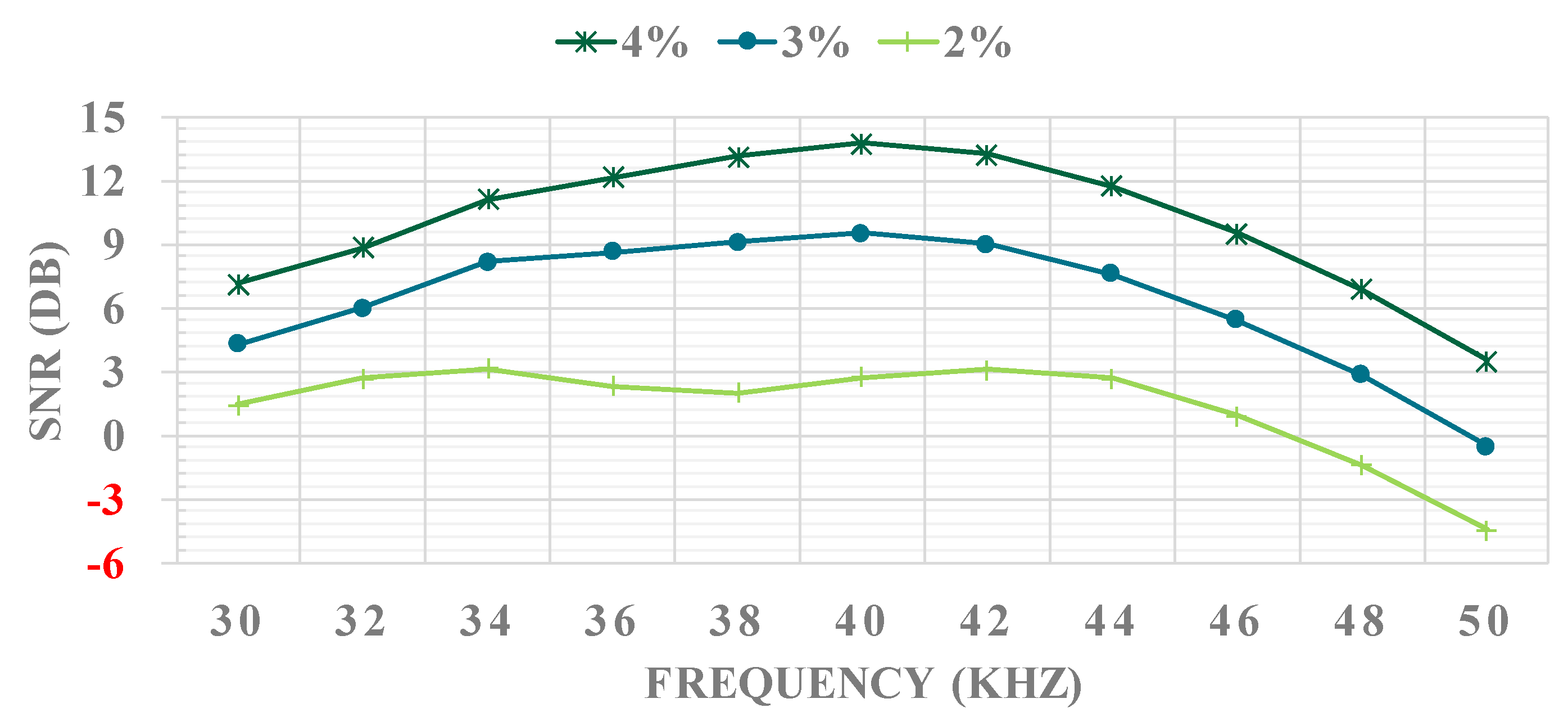
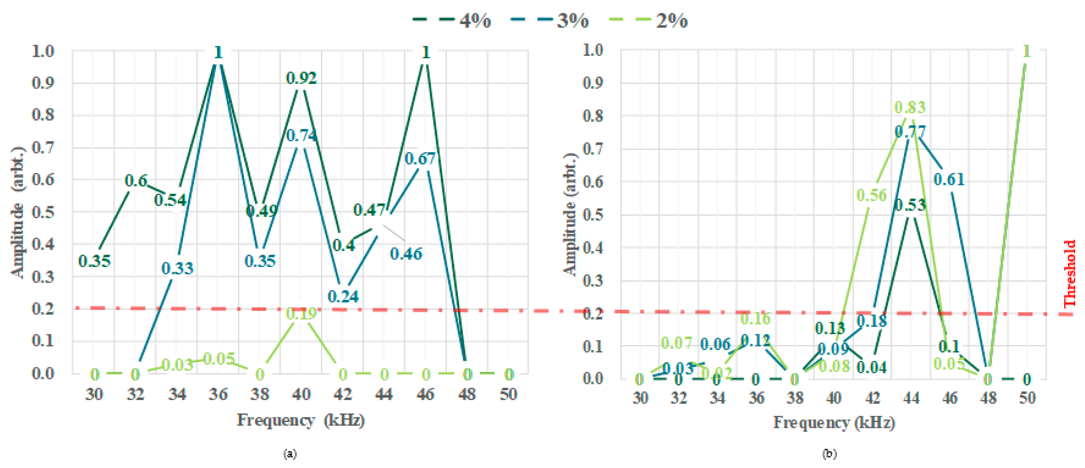
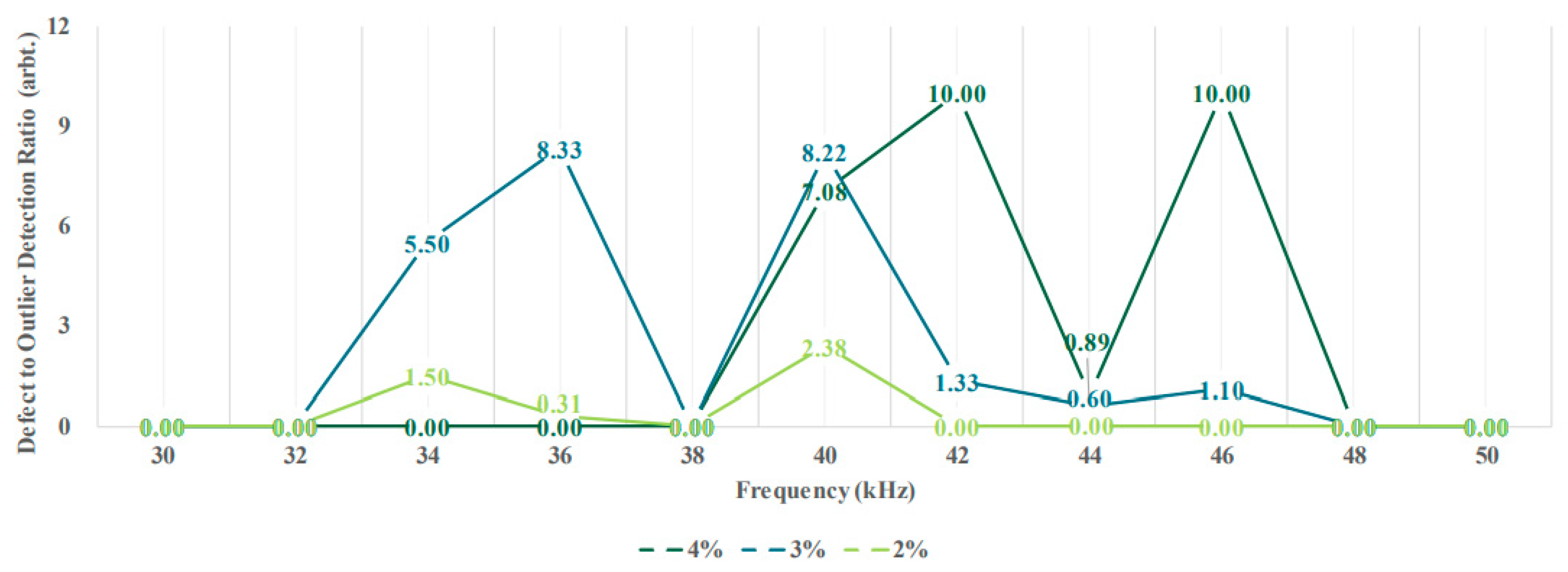
The algorithm was initially developed and validated on synthesised data from FEM. Afterwards, experimental data form real pipes with defect CSA sizes of 2, 3 and 4%, were used to validate its capability and also its limitations. It was illustrated that the choice of excitation frequency is a trade-off between the ability of the system to generate the given excitation sequence and having highly dispersive flexural waves (which are considered as the main source of the noise in these tests). As such, it was observed that frequencies in the range of 34 to 40 kHz are optimal, and can detect defects reliabily with larger CSA sizes than 3% with no or very few outliers. In the case of 2% CSA defect, only frequencies of 34 and 40 kHz provided robust detection, where the ratio of the defect to outlier amplitudes is higher by a factor of 1.5. On the other hand, 38 kHz is the only frequency within this range where no outliers were detected in any of the cases. With regards to the test results, due to the significant changes in the excitation sequences, it is not recommended to use this algorithm with frequencies higher than 42 kHz. Since this method only requires a time-domain signal and the characteristics of the excitation sequence, it can easily be combined with other methods to further enhance the reliability of defect detection in guided-wave testing of pipelines.