Article

Robust Backstepping Trajectory Tracking Control of a Quadrotor with Input Saturation via Extended State Observer

Faculty of Mechanical and Aerospace Engineering, Sejong University, Seoul 05006, Korea
*
Author to whom correspondence should be addressed.
Appl. Sci. 2019, 9(23), 5184; https://doi.org/10.3390/app9235184
Submission received: 8 October 2019 / Revised: 29 October 2019 / Accepted: 20 November 2019 / Published: 29 November 2019
(This article belongs to the Special Issue Unmanned Aerial Vehicles (UAVs))

Abstract

:
Quadrotor unmanned aerial vehicles have become increasingly popular in several applications, and the improvement of their control performance has been documented in several studies. Nevertheless, the design of a high-performance tracking controller for aerial vehicles that reliably functions in the simultaneous presence of model uncertainties, external disturbances, and control input saturation still remains a challenge. In this paper, we present a robust backstepping trajectory tracking control of a quadrotor with input saturation. The controller design accounts for both parameterized uncertainties and external disturbances, whereas a new auxiliary system is proposed to cope with control input saturation. Taking into account that only the position and attitude of the quadrotor are measurable, we devise an extended state observer to supply the estimations of unmeasured states, model uncertainties, and external disturbances. We strictly prove the stability of the closed-loop system by using the Lyapunov theory and demonstrate the effectiveness of the proposed algorithm through numerical simulations.

1. Introduction

In recent years, unmanned aerial vehicles (UAVs) have been used in a broad range of applications that include scientific research, civil engineering, military applications, aerial mapping, search and rescue operations, and risk zone inspections [1]. Quadrotors are an important class of UAVs that has attracted a great deal of attention from scientists and engineers due to their numerous advantages such as rapid maneuverability, diverse applicability, reliability, and economy [2,3,4]. However, the quadrotor is a typical example of a coupled underactuated system, as it has six degrees of freedom but only four control inputs. In addition, there are parameterized uncertainties in the quadrotor’s rigid body dynamics and aerodynamics which further complicate the design of a high-performance controller. Furthermore, the presence of external disturbances and control input saturation pose a significant challenge to solving the quadrotor’s trajectory tracking control (TTC) problem. Meanwhile, the TTC is pivotal to many quadrotor’s applications including multi-agent coordination [5], efficient obstacle avoidance [6], and autonomous docking. Therefore, the design of a robust adaptive trajectory tracking controller for quadrotors has become a pressing issue in the scientific community.
Several studies have aimed at improving the performance of the quadrotor trajectory tracking control. In [7], the authors proposed a hierarchical flight control scheme using multiple proportional-integral-derivative (PID) controller loops to address the three dimensional (3D) TTC problem. The authors of [8] designed a tracking controller by combining a PID controller and a backstepping controller. The backstepping control technique was also applied in [9,10] to accomplish the TTC of quadrotors. The H control method was applied in [11] to solve the output tracking control problem. Another approach was taken in [12], where the authors employed a state space predictive controller to track some predefined trajectories in combination with an H controller to stabilize the vehicle’s rotational movements. In [13,14], TTC was achieved by applying the sliding mode control (SMC) technique. Yet another tracking controller based on the model-predictive control method was investigated in [15].
Although all the above approaches employ advanced control techniques, they all suffer from the same shortcoming: they all have system parameters and unknown external disturbances that are unaccounted for. To overcome this problem, several quadrotor control methods were investigated such as fuzzy, intelligent control, dynamic surface control, backstepping control, etc. [16,17]. In [18], the authors presented a novel approximate dynamic programming deep learning algorithm for enabling a quadrotor systems to perform a trajectory tracking in the presence of adversarial inputs. In [19], a neurobiologically inspired intelligent algorithm for quadrotor systems was introduced to achieve the TTC under the presence of uncertain system dynamics and disturbances. Another neural network based intelligent control method was also developed in approach [20] to stabilize a quadrotor system under complex environment including system uncertainties and/or disturbances. These methods [18,19,20] can deliver a satisfactory control performance, but require considerable computational resources. Meanwhile, many studies have focused on disturbance–observer (DO)-based tracking controllers to accomplish a robust control performance. Although the authors of [21,22,23] investigated backstepping controllers based on a DO and demonstrated good tracking performance, the authors of [24,25,26] devised DO-based tracking sliding mode controllers. High gain observers and robust controllers to deal with the tracking problem have also been presented in [27,28]. However, all the control strategies in [21,22,23,24,25,26,27,28], especially with regard to the backstepping controllers, require full-state measurements that may not be possible due to insufficient sensor numbers and/or sensor faults.
In response, quadrotor researchers have proposed many solutions that either maintain the control performance or reduce the mass and cost of the vehicle by utilizing only partial state measurements. In [29,30], based on a reduced-order observer, the authors presented robust TTC algorithms without using linear velocity measurements.The authors of [31] introduced an active disturbance rejection and predictive control strategy to deal with the tracking problem in the presence of disturbances in six degrees of freedom. The controller can guarantee a smooth tracking performance while employing only position and attitude measurements. Tracking controllers based on the hierarchical control strategy without linear velocity and angular velocity measurements are presented in [32,33]. Yet another robust backstepping tracking controller using an extended state observer (ESO) to estimate unmeasurable states and disturbances from only position measurements was proposed in [34]. In [35], an ESO was used to supply estimations of internal states and external disturbances that are used by a target tracking backstepping controller and an attitude stabilized controller. The ESO has also been used in the design of controllers for a helicopter [36], fixed-wing airplane [37], spacecraft [38], and missile [39].
From a practical point of view, control input saturation occurs frequently and has a significant effect on a system’s control performance degradation. To address this problem, the authors of [40] presented a quadrotor backstepping-based controller under input saturation. However, this approach cannot achieve TTC as it considers only attitude stabilization. Two different approaches to solve the tracking problem used a hierarchical inner–outer loop controller [41] or a linear quadratic regulator (LQR) [42]. However, both approaches are not sufficiently robust against disturbances. Once it was realized that input saturation further exacerbates the control problem of perturbed systems, the robust adaptive control problem with input saturation has been investigated. For example, in [43], the authors proposed an adaptive and robust saturated control to achieve the TTC of quadrotors under the presence of disturbances. Robust saturated tracking controllers were also presented in [44,45,46], with [44,45] using a backstepping-based controller, whereas the work in [46] is based on the SMC technique. However, these studies [43,44,45,46] require the full-state information from the sensor systems, which is not always possible to achieve.
From the above observations, it is seen that the backstepping control technique plays important roles in solving the TTC of quadrotors. In addition, the references indicate that most of the previous studies are only capable of solving the TTC partially under the comprehensive presence of parameterized uncertainties, external disturbances, and control input saturation. The TTC still needs to be addressed to meet the higher control performance requirements posed by real-world applications. In this paper, we propose a novel ESO-based robust backstepping trajectory tracking controller for quadrotor under control input saturation which advances the current state of the art in three ways:
(i) Unlike previous saturated control studies in [43,44,46], our method does not require full-state information of the system: partial state knowledge is sufficient. In addition, our approach can account for the presence of lumped disturbances (consisting of parameterized uncertainties and external disturbances) in both the translational and rotational dynamics of the quadrotor. In several studies of quadrotor [47,48], achieving the TTC mission is difficult, as only the vehicle’s position and attitude are provided by sensors. Based on the assumption that only the position and attitude of the quadrotor are known, we devise an ESO to supply estimations of velocity, angular rate states, and the lumped disturbances.
(ii) We devise a robust backstepping TTC algorithm to achieve the tracking control task in the presence of lumped disturbances and control input saturation. This contribution is clearly superior to the reduced-order observer based control approaches presented in [30,31,32,33,34,35,36,37,38,39,40,41,42], which can only achieve a partial solution of the robust adaptive saturated tracking control problem. To overcome the problem of “explosion of complexity”, which is generally problematic in integrator backstepping control, dynamic filters (also referred to as linear tracking differentiator [49]) are applied to compute the derivative of virtual control signals.
(iii) We use the Lyapunov theory to verify the stability of the closed-loop system and prove that both the ESO estimation errors as well as tracking errors are ultimately bounded, despite the presence of lumped disturbances and control input saturation.
The remainder of this paper is organized as follows. Section 2 presents the quadrotor dynamics model and problem formulation. Section 3 contains the design and stability analysis of an ESO. Based on the devised ESO, a robust trajectory backstepping saturated controller is proposed in Section 4. The stability of the closed-loop system is analyzed in Section 5. Numerical simulation results and discussions are provided in Section 6, before ending with overall conclusions in Section 7.

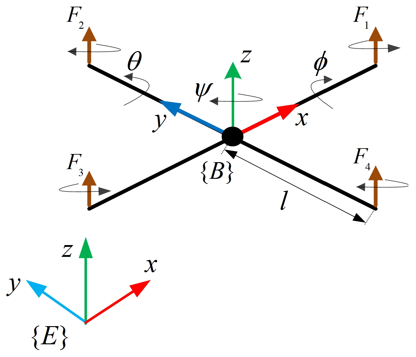
2. Quadrotor Dynamics Model and Problem Formulation

In this section, we briefly present the quadrotor dynamics model, as it was clearly introduced and verified in many previous studies [34,43,50,51].
Figure 1 illustrates the quadrotor configuration. The four rotors of the quadrotor generate four thrust forces F i ( i = 1 , , 4 ) that have relationship with the control inputs as
u 1 = F 1 + F 2 + F 3 + F 4 u 2 = F 2 - F 4 u 3 = F 3 - F 1 u 4 = - F 1 + F 2 - F 3 + F 4
The cascaded dynamics model of the quadrotor is described as
m P ¨ = - Λ 1 P ˙ - G + B 1 u 1 + d 1 ( t ) J Θ ¨ = - Λ 2 Θ ˙ + B 2 U 2 + d 2 ( t )
where P = [ x , y , z ] T and Θ = [ ϕ , θ , ψ ] T , respectively, denote the position and attitude of quadrotor in the inertial frame E. m R + the mass. G = [ 0 , 0 , m g ] T with g being the gravitational acceleration. J = d i a g ( J 1 , J 2 , J 3 ) R 3 × 3 the nominal inertia momentum matrix. Λ 1 = d i a g ( λ x , λ y , λ z ) and Λ 2 = d i a g ( λ ϕ , λ θ , λ ψ ) represent the damping matrices, with λ i ( i = x , y , , ψ ) being nominal drag coefficients. B 1 = [ c ( ϕ ) s ( θ ) c ( ψ ) + s ( ϕ ) s ( ψ ) , s ( ϕ ) s ( θ ) c ( ψ ) - c ( ϕ ) s ( ψ ) , c ( ϕ ) c ( θ ) ] T the input matrix of position subsystem, where s ( x ) , c ( x ) is an abbreviation for sin ( x ) , cos ( x ) , respectively. B 2 = d i a g ( l , l , c d ) is a symmetric positive definite constant matrix, where l , c d are the quadrotor arm length and nominal force-to-moment coefficients, respectively. u 1 R and U 2 = [ u 2 , u 3 , u 4 ] T the control inputs. d 1 ( t ) and d 2 ( t ) are the lumped disturbances, including parameterized uncertainties and external disturbances, in position and orientation dynamics, respectively.
To take the control input saturation into account, the control input vector [ u 1 , u 2 , u 3 , u 4 ] T is restricted by sat ( u ) with
sat ( u ) = sat ( u 1 ) sat ( u 2 ) sat ( u 3 ) sat ( u 4 )
where
s a t ( u i ) = u i max , u i > u i max u i , - u i max u i u i max , ( i = 1 , , 4 ) - u i max , u i < - u i max
with u i max being the maximum control authority in the i-th component that can be provided by the actuators.
To address the observer and controller design, the quadrotor dynamics model (2) is transformed into the augmented dynamics in translational and rotational loops as
X ˙ 1 = X 2 X ˙ 2 = - Λ 1 X 2 / m + ( B 1 u 1 - G ) / m + X 3 X ˙ 3 = h p X ˙ 4 = X 5 X ˙ 5 = - J - 1 Λ 2 X 5 + J - 1 B 2 U 2 + X 6 X ˙ 6 = h θ
where the system state variables are denoted as X 1 = P , X 2 = P ˙ , X 4 = Θ , and X 5 = Θ ˙ . We extend the lumped disturbances as additional state variables of the system with X 3 = d 1 ( t ) / m and X 6 = J - 1 d 2 ( t ) . In addition, we define X ˙ 3 = h p and X ˙ 6 = h θ , with h p and h θ representing the bounded derivative of the lumped disturbances and satisfying h p H 1 and h θ H 2 , where represents the 2-norm, and H 1 and H 2 are some positive numbers.
For the sake of simplicity, let us present the following notations before moving forward.
f 2 ( X 2 ) = - Λ 1 X 2 / m , F ( X 4 ) = ( B 1 u 1 - G ) / m , f 5 ( X 5 ) = - J - 1 Λ 2 X 5 , B 5 = J - 1 B 2
Here, note that F becomes a virtual control vector to be designed later.
Then, we can rewrite Equation (5) as
X ˙ 1 = X 2 X ˙ 2 = X 3 + f 2 ( X 2 ) + F ( X 4 ) X ˙ 3 = h p X ˙ 4 = X 5 X ˙ 5 = X 6 + f 5 ( X 5 ) + B 5 U 2 X ˙ 6 = h θ
In the matrix form, system Equation (6) can be rewritten as
X ˙ = A 0 X + Φ ( X ) + U + Δ
where, we use the following notations,
X = X 1 X 2 X 3 X 4 X 5 X 6 , A 0 = 0 I 3 0 0 0 0 0 0 I 3 0 0 0 0 0 0 0 0 0 0 0 0 0 I 3 0 0 0 0 0 0 I 3 0 0 0 0 0 0 , Φ ( X ) = 0 f 2 ( X 2 ) 0 0 f 5 ( X 5 ) 0 , U = 0 F ( X 5 ) 0 0 B 5 U 2 0 , Δ = 0 0 h p 0 0 h θ
where I 3 R 3 × 3 stands for an identity matrix, and 0 is a zero matrix or zero vector with proper dimensions.
Now, the control goal is to design a robust backstepping trajectory tracking controller to steer the quadrotor to a given trajectory reference P d and a desired heading angle ψ d using only the measurements of position and attitude, i.e., X 1 and X 4 , despite the presence of both control input saturation and the lumped disturbances.

3. Extended State Observer

As only the vehicle’s position and attitude are known, an ESO is devised to supply estimates of velocity, angular rate states, and the lumped disturbances. Following the principle of high-gain observer design [52], the ESO is formulated as
X ^ ˙ = A 0 X ^ + Φ ( X ^ ) + U ^ + H X 1 - X ^ 1 X 4 - X ^ 4
with
  • X ^ = X ^ 1 X ^ 2 X ^ 3 X ^ 4 X ^ 5 X ^ 6 T ,
  • Φ ( X ^ ) = 0 f 2 ( X ^ 2 ) 0 0 f 5 ( X ^ 5 ) 0 T ,
  • U ^ = 0 F ( X ^ 4 ) 0 0 B 5 U 2 0 T ,
  • H = 3 ω 1 I 3 3 ω 1 2 I 3 ω 1 3 I 3 0 0 0 0 0 0 3 ω 2 I 3 3 ω 2 2 I 3 ω 2 3 I 3 T ,
where X ^ i ( i = 1 , , 6 ) is the estimated value of X i , H denotes the observer gain matrix, and ω 1 , ω 2 are the ESO’s bandwidth parameters.
To begin the analysis of the ESO’s stability, let us define the estimation error X ˜ as
X ˜ = X - X ^ = X ˜ 1 X ˜ 2 X ˜ 3 X ˜ 4 X ˜ 5 X ˜ 6 T
Then, the corresponding scaled estimation error is defined as
ϑ = ϑ 1 ϑ 2 ϑ 3 ϑ 4 ϑ 5 ϑ 6 T = X ˜ 1 ω 1 2 X ˜ 2 ω 1 X ˜ 3 X ˜ 4 ω 2 2 X ˜ 5 ω 2 X ˜ 6 T
By recalling Equations (7) and (8), we obtain the scaled estimation error dynamics as
ϑ ˙ = ω A ϑ + ω 1 δ 2 [ f 2 ( X 2 ) - f 2 ( X ^ 2 ) + F ( X 4 ) - F ( X ^ 4 ) ] + δ 3 h p + ω 2 δ 5 [ f 5 ( X 5 ) - f 5 ( X ^ 5 ) ] + δ 6 h θ = ω A ϑ + ω 1 δ 2 ( f 2 ˜ + F ˜ ) + δ 3 h p + ω 2 δ 5 f 5 ˜ + δ 6 h θ
where
  • ω = ω 1 I 9 0 0 ω 2 I 9 ,
  • A = - 3 I 3 I 3 0 0 0 0 - 3 I 3 0 I 3 0 0 0 - I 3 0 0 0 0 0 0 0 0 - 3 I 3 I 3 0 0 0 0 - 3 I 3 0 I 3 0 0 0 - I 3 0 0 ,
  • δ 2 = 0 I 3 0 0 0 0 T , δ 3 = 0 0 I 3 0 0 0 T , δ 5 = 0 0 0 0 I 3 0 T ,
  • δ 6 = 0 0 0 0 0 I 3 T f 2 ˜ = f 2 ( X 2 ) - f 2 ( X ^ 2 ) , f 5 ˜ = f 5 ( X 5 ) - f 5 ( X ^ 5 ) .
Before moving on, it is necessary to introduce the following assumption that is widely used in the proof of ESO’s stability.
Assumption 1 ([34,53]). The functions F , f 2 , and f 5 are globally Lipschitz in their auguments, i.e., there exist positive numbers γ 1 , γ 2 , γ 5 such that
F ( X 4 ) - F ( X ^ 4 ) γ 1 ϑ 4 γ 1 ϑ f 2 ( X 2 ) - f 2 ( X ^ 2 ) γ 2 ϑ 2 γ 2 ϑ f 5 ( X 5 ) - f 5 ( X ^ 5 ) γ 5 ϑ 5 γ 5 ϑ
for all X i , X ^ i ( i = 2 , 4 , 5 ) .
Theorem 1.
Consider the ESO’s estimation error dynamics in Equation (10), let P be the positive definite symmetric matrix satisfying A T P + P A = - I 18 for the Hurwitz matrix A defined, if the observer bandwidths ω 1 and ω 2 are designated such that α = ω m - 2 ω 1 γ 1 μ 2 - 2 ω 1 γ 2 μ 2 - 2 ω 2 γ 5 μ 5 > 0 with ω m = m i n { ω 1 , ω 2 } and μ i = P δ i ( i = 2 , 3 , 5 , 6 ) , then the ESO is stable and the estimation error is ultimately bounded and asymptotically approach to the origin.
Proof. 
Choose a Lyapunov candidate function as
V 1 ( ϑ ) = ϑ T P ϑ
Thus, we have
λ m i n ( P ) ϑ 2 V 1 λ m a x ( P ) ϑ 2
where λ m i n ( P ) and λ m a x ( P ) are minimum and maximum eigenvalues of P , respectively.
The time derivative of V 1 is
V ˙ 1 ( ϑ ) = ϑ T P ϑ ˙ + ϑ ˙ T P ϑ = ϑ T P [ ω A ϑ + ω 1 δ 2 ( f 2 ˜ + F ˜ ) + δ 3 h p + ω 2 δ 5 f 5 ˜ + δ 6 h θ ] + [ ω A ϑ + ω 1 δ 2 ( f 2 ˜ + F ˜ ) + δ 3 h p + ω 2 δ 5 f 5 ˜ + δ 6 h θ ] T P ϑ = ϑ T ( P ω A + A T ω T P ) ϑ + 2 ω 1 ϑ T P δ 2 ( f 2 ˜ + F ˜ ) + 2 ω 2 ϑ T P δ 5 f 5 ˜ + 2 ϑ T P δ 3 h p + 2 ϑ T P δ 5 h θ - ω m ϑ 2 + 2 ω 1 ( γ 1 + γ 2 ) ϑ T P δ 2 ϑ + 2 ω 2 γ 5 ϑ T P δ 5 ϑ + 2 H 1 ϑ T P δ 3 + 2 H 2 ϑ P δ 6 - ( ω m - 2 ω 1 γ 1 μ 2 - 2 ω 1 γ 2 μ 2 - 2 ω 2 γ 5 μ 5 ) ϑ 2 + 2 ( H 1 μ 3 + H 2 μ 6 ) ϑ - ω m - 2 ω 1 γ 1 μ 2 - 2 ω 1 γ 2 μ 2 - 2 ω 2 γ 5 μ 5 λ m a x ( P ) V 1 + 2 ( H 1 μ 3 + H 2 μ 6 ) λ m i n ( P ) V 1 - α λ m a x ( P ) V 1 + 2 β λ m i n ( P ) V 1
where β = H 1 μ 3 + H 2 μ 6 .
To obtain a linear differential inequality from Equation (14), let us introduce the following function.
W 1 ( t ) = V 1
Then, when V 1 0 , we have
W ˙ 1 ( t ) = V ˙ 1 2 V 1 - α 2 λ m a x ( P ) W 1 + β λ m i n ( P )
Following the comparison principle [52], the following inequality can be derived from Equation (16).
W 1 [ W 1 ( 0 ) - C 0 ] exp [ - α 2 λ m a x ( P ) t ] + C 0
where
C 0 = 2 λ m a x ( P ) β α λ m i n ( P )
Invoking (13), one obtains the upper bound of ϑ as
ϑ V 1 ( 0 ) - C 0 λ m i n ( P ) exp [ - α 2 λ m a x ( P ) t ] + C 0 λ m i n ( P )
Then, we have:
lim sup t ϑ C = 2 λ m a x ( P ) β α λ m i n ( P )
From the above analysis, it is clear that ϑ is uniformly ultimately bounded. Consequently, from Equation (9), the ultimate upper bound of the scaled estimation error is
lim sup t X ˜ 1 C / ω 1 2 , lim sup t X ˜ 2 C / ω 1 , lim sup t X ˜ 3 C , lim sup t X ˜ 4 C / ω 2 2 , lim sup t X ˜ 5 C / ω 2 , lim sup t X ˜ 6 C
From Equation (21), it can be clearly concluded that when the observer bandwidth parameters are sufficiently large, the ESO is stable and its state variables can reach their real values with arbitrarily small estimation errors. This fact implies that
lim ω m C = lim ω m 2 λ m a x ( P ) β α λ m i n ( P ) = 0
 □
Remark 1.
Equations (20) and (21) indicate that increasing the bandwidth parameters ω 1 and ω 2 can improve the estimation accuracy of the ESO. However, from Equation (8), it can be seen that any tiny measurement uncertainties of X 1 and X 4 will be excessively amplified if the bandwidth parameters are too large. Therefore, the bandwidth parameters should be tuned appropriately to make a trade-off between the estimation accuracy and the robustness of the ESO.

4. Robust Saturated Backstepping Tracking Controller Design

In this section, an ESO-based backstepping controller is presented for addressing the robust trajectory tracking control problem of quadrotors in the presence of both the system parameterized uncertainties in combination with external disturbances and control input saturation. With the application of the ESO proposed in Section 3, the estimates of velocity, angular rate, and the lumped disturbances in both translational and rotational dynamics are supplied simultaneously and, thus, can be used in the following controller design procedures.
Let us define the position tracking error as the subtraction of the actual position vector, X 1 , from the desired position vector, P d :
e 1 = X 1 - P d
Thus, the derivative of e 1 is
e ˙ 1 = X 2 - P ˙ d
A virtual control law for (24) is constructed as
X ¯ 2 = - k 1 ( X 1 - P d ) + P ˙ d
where k 1 R + is a controller gain. The approximation of X ¯ ˙ 2 is computed by making use of the following first-order low-pass filter (LPF) [54],
τ 2 X ˙ 2 f + X 2 f = X ¯ 2
where τ 2 R + . Then,
X ¯ ˙ 2 = X ˙ 2 f + ϵ 2
with the approximation error ϵ 2 satisfying ϵ 2 E 2 R + .
Next, we consider the velocity tracking error as
e 2 = X 2 - X ¯ 2
Taking derivative of e 2 gives
e ˙ 2 = X ˙ 2 - X ¯ ˙ 2 = X 3 + f 2 ( X 2 ) + F ( X 4 ) - X ¯ ˙ 2
To address the control input saturation corresponding to u 1 , let us consider the following Lyapunov candidate function,
V 2 = 1 2 ( e 2 - ξ 1 ) T ( e 2 - ξ 1 ) + 1 2 ξ 1 T ξ 1
where, ξ 1 is an auxiliary variable relating to the control input saturation and its dynamics will be designed later. Differentiating Equation (30) yields
V ˙ 2 = ( e 2 - ξ 1 ) T ( e ˙ 2 - ξ ˙ 1 ) + ξ 1 T ξ ˙ 1
Substituting Equation (29) into (31) gives
V ˙ 2 = ( e 2 - ξ 1 ) T ( X 3 + f 2 ( X 2 ) + F ( X 4 ) - X ¯ ˙ 2 - ξ ˙ 1 ) + ξ T ξ ˙
For the V ˙ 2 to be negative definite, the virtual control vector F and the dynamics of ξ 1 are designed as
F = - f 2 ( X ^ 2 ) - k 2 ( X ^ 2 - X ¯ 2 - ξ 1 ) - X ^ 3 + X ˙ 2 f + ξ ˙ 1 ξ ˙ 1 = - k 3 ξ 1 + Δ F
where k 2 , k 3 R + and Δ F = sat ( F ) - F . Here, note that F ( X 4 ) = ( B 1 u 1 - G ) / m and assuming that Δ F satisfies Δ F υ 1 with υ 1 R + .
Now, the thrust force u 1 and the desired values of roll and pitch angles, i.e., ϕ d and θ d , can be calculated from the following equation.
F = F 1 F 2 F 3 = u 1 m [ c ( ϕ d ) s ( θ d ) c ( ψ d ) + s ( ϕ d ) s ( ψ d ) ] u 1 m [ s ( ϕ d ) s ( θ d ) c ( ψ d ) - c ( ϕ d ) s ( ψ d ) ) ] u 1 m [ c ( ϕ d ) c ( θ d ) ] - g
Here, the desired heading angle ψ d is determined by some high-level guidance algorithm that will not be discussed as it is beyond the scope of this paper. Manipulating (34) yields
u 1 = m F 1 2 + F 2 2 + ( F 3 + g ) 2 ϕ d = arcsin ( m u 1 [ F 1 sin ( ψ d ) - F 2 cos ( ψ d ) ] ) θ d = arctan ( 1 F 3 + g [ F 1 cos ( ψ d ) + F 2 sin ( ψ d ) ] )
Let e 4 denote attitude tracking error as
e 4 = X 4 - X ¯ 4
with X ¯ 4 = [ ϕ d , θ d , ψ d ] being a virtual control law.
Then, the derivative of e 4 can be obtained as
e ˙ 4 = X ˙ 4 - X ¯ ˙ 4 = X 5 - X ¯ ˙ 4
A virtual control law for (37) is constructed as
X ¯ 5 = - k 4 ( X ^ 4 - X ¯ 4 ) + X ¯ ˙ 4
where k 4 R + is a controller gain.
Thus, the angular rate tracking error is defined as
e 5 = X 5 - X ¯ 5
The following LPF is applied to compute the approximation of X ¯ ˙ 5 ,
τ 5 X ˙ 5 f + X 5 f = X ¯ 5
where τ 5 R + . Then,
X ¯ ˙ 5 = X ˙ 5 f + ϵ 5
with the approximation error ϵ 5 satisfying ϵ 5 E 5 R + .
Taking derivative of (39), we have
e ˙ 5 = X ˙ 5 - X ¯ ˙ 5 = X 6 + f 5 ( X 5 ) + B 5 U 2 - X ¯ ˙ 5
To address the control input saturation corresponding to U 2 , let us consider the following Lyapunov candidate function,
V 3 = 1 2 ( e 5 - ξ 2 ) T ( e 5 - ξ 2 ) + 1 2 ξ 2 T ξ 2
where, ξ 2 is an auxiliary variable relating to the input saturation and its dynamics will be designed later. Differentiating Equation (37) yields
V ˙ 3 = ( e 5 - ξ 2 ) T ( e ˙ 5 - ξ ˙ 2 ) + ξ 2 T ξ ˙ 2
Substituting Equation (36) into (38) gives
V ˙ 3 = ( e 5 - ξ 2 ) T ( X 6 + f 5 ( X 5 ) + B 5 U 2 - X ¯ ˙ 5 - ξ ˙ 2 ) + ξ 2 T ξ ˙ 2
To achieve the V ˙ 3 negative definite, the control vector U 2 and the dynamics of ξ 2 are designed as
U 2 = B 5 - 1 [ - f 5 ( X ^ 5 ) - k 5 ( X ^ 5 - X ¯ 5 - ξ 2 ) - X ^ 6 + X ˙ 5 f + ξ ˙ 2 ] ξ ˙ 2 = - k 6 ξ 2 + Δ U 2
where k 5 , k 6 R + and Δ U 2 = sat ( U 2 ) - U 2 . Assume that Δ U 2 satisfies Δ U 2 υ 2 with υ 2 R + .

5. Closed-Loop System’s Stability Analysis

In this section, we move on establishing the stability analysis of the closed-loop system. Toward that end, the error dynamics of the closed-loop system needs to be derived first. By combining Equation (10) with the equations from (23) to (46), we have the following formula.
e ˙ 1 = X 2 - P ˙ d = ( X 2 - X ¯ 2 ) + X ¯ 2 - P ˙ d = - k 1 e 1 + e 2
e ˙ 2 = X 3 + f 2 ( X 2 ) + F ( X 4 ) - X ¯ ˙ 2 = X 3 + f 2 ( X 2 ) - f 2 ( X ^ 2 ) - k 2 ( X ^ 2 - X ¯ 2 - ξ 1 ) - X ^ 3 + X ˙ 2 f - k 3 ξ 1 + Δ F - X ¯ ˙ 2 = - k 2 ( e 2 - ξ 1 ) + f 2 ˜ + k 2 ϑ 2 ω 1 + ϑ 3 - k 3 ξ 1 + Δ F - ϵ 2
e ˙ 4 = ( X 5 - X ¯ 5 ) + X ¯ 5 - X ¯ ˙ 4 = e 5 - k 4 ( X ^ 4 - X ¯ 4 ) = e 5 - k 4 ( e 4 + X ˜ 4 ) = - k 4 e 4 + e 5 + k 4 ϑ 4 ω 2 2
e ˙ 5 = X 6 + f 5 ( X 5 ) - f 5 ( X ^ 5 ) - k 5 ( X ^ 5 - X ¯ 5 - ξ 2 ) - X ^ 6 + X ˙ 5 f + ξ ˙ 2 - X ¯ ˙ 5 = X ˜ 6 + f ˜ 5 - k 5 ( e 5 - ξ 2 ) + k 5 X ˜ 5 - k 6 ξ 2 + Δ U 2 - ϵ 5 = - k 5 ( e 5 - ξ 2 ) + f ˜ 5 + k 5 ϑ 5 ω 2 + ϑ 6 - k 6 ξ 2 + Δ U 2 - ϵ 5
From Equations (47)–(50), the closed-loop system’s error dynamics can be written as
e ˙ 1 = - k 1 e 1 + e 2 e ˙ 2 = ϑ 3 + f 2 ˜ - k 2 ( e 2 - ξ 1 ) + k 2 ϑ 2 ω 1 - k 3 ξ 1 + Δ F - ϵ 2 ξ ˙ 1 = - k 3 ξ 1 + Δ F e ˙ 4 = - k 4 e 4 + e 5 + k 4 ϑ 4 ω 2 2 e ˙ 5 = - k 5 ( e 5 - ξ 2 ) + k 5 ϑ 5 ω 2 + f ˜ 5 + ϑ 6 - k 6 ξ 2 + Δ U 2 - ϵ 5 ξ ˙ 2 = - k 6 ξ 2 + Δ U 2 ϑ ˙ = ω A ϑ + ω 1 δ 2 ( f 2 ˜ + F ˜ ) + δ 3 h p + ω 2 δ 5 f 5 ˜ + δ 6 h θ
Theorem 2.
Consider the quadrotor dynamics as described in Equation (2), for the given sufficiently smooth trajectory command P d and heading angle ψ d , if the controller gains k i ( i = 1 , , 6 ) and the observer bandwidth parameters ω 1 , ω 2 are chosen such that the matrix Π defined in the following is positive definite, then the ESO-based saturated trajectory tracking controller, including the virtual controllers (25), (33), (38), and (46) and the applied controllers (35) and (46), can guarantee the ultimate boundedness of all signals in the closed-loop and make the tracking errors arbitrarily small.
Π = Π 1 Π 2 Π 2 T Π 3 Π 1 = k 1 - 1 2 - 1 2 0 0 0 - 1 2 k 2 - c 4 2 0 0 0 0 - 1 2 0 k 3 - c 1 2 0 0 0 0 0 0 k 4 - 1 2 - 1 2 0 0 0 - 1 2 k 5 - c 5 2 0 0 0 0 - 1 2 0 k 6 - c 2 2 Π 2 = 0 0 0 0 0 0 0 - 1 2 ( γ 2 + k 2 ω 1 ) - 1 2 0 0 0 0 0 0 0 0 0 0 0 0 - k 4 2 ω 2 2 0 0 0 0 0 0 - 1 2 ( γ 5 + k 5 ω 2 ) - 1 2 0 0 0 0 0 0 Π 3 = ( α 2 - c 3 4 ) d i a g ( 1 , 1 , 1 , 1 , 1 , 1 )
with c j ( j = 1 , , 5 ) being some positive constants to be chosen.
Proof. 
Consider the following Lyapunov candidate function
V = 1 2 e 1 T e 1 + 1 2 ( e 2 - ξ 1 ) T ( e 2 - ξ 1 ) + 1 2 ξ 1 T ξ 1 + 1 2 e 4 T e 4 + 1 2 ( e 5 - ξ 2 ) T ( e 5 - ξ 2 ) + 1 2 ξ 2 T ξ 2 + 1 2 ϑ T P ϑ
Substituting (10) and (51) into the time derivative of V gives
V ˙ e 1 T ( - k 1 e 1 + e 2 ) + ( e 2 - ξ 1 ) T [ - k 2 ( e 2 - ξ 1 ) + f 2 ˜ + ϑ 3 - ϵ 2 + k 2 ϑ 2 ω 1 ] + ξ 1 T ( - k 3 ξ 1 + Δ F ) + e 4 T ( - k 4 e 4 + e 5 + k 4 ϑ 4 ω 2 2 ) + ( e 5 - ξ 2 ) T [ - k 5 ( e 5 - ξ 2 ) + k 5 ϑ 5 ω 2 + f ˜ 5 + ϑ 6 - ϵ 5 ] + ξ 2 T ( - k 6 ξ 2 + Δ U 2 ) - 1 2 ω m ϑ 2 + ( ω 1 γ 1 μ 2 + ω 1 γ 2 μ 2 + ω 2 γ 5 μ 5 ) ϑ 2 + μ 3 ϑ h p + μ 5 ϑ h θ - k 1 e 1 T e 1 - k 2 ( e 2 - ξ 1 ) T ( e 2 - ξ 1 ) - k 3 ξ 1 T ξ 1 - k 4 e 4 T e 4 - k 5 ( e 5 - ξ 2 ) T ( e 5 - ξ 2 ) - k 6 ξ 2 T ξ 2 + ( e 2 - ξ 1 ) T ( f 2 ˜ + k 2 ω 1 ϑ 2 ) + ( e 2 - ξ 1 ) T ϑ 3 + k 4 ω 2 2 e 4 T ϑ 4 + ( e 5 - ξ 2 ) T ( f ˜ 5 + k 5 ω 2 ϑ 5 ) + ( e 5 - ξ 2 ) T ϑ 6 + e 1 T e 2 - ( e 2 - ξ 1 ) T ϵ 2 - ( e 5 - ξ 2 ) T ϵ 5 + e 4 T e 5 + ξ 1 T Δ F + ξ 2 T Δ U 2 - α 2 ϑ 2 + β ϑ
Obviously, we have the following relationship.
e 1 T e 2 = e 1 T ( e 2 - ξ 1 ) + e 1 T ξ 1 e 1 e 2 - ξ 1 + e 1 ξ 1 e 4 T e 5 = e 4 T ( e 5 - ξ 2 ) + e 4 T ξ 2 e 4 e 5 - ξ 2 + e 4 ξ 2 ξ 1 T Δ F c 1 2 ξ 1 2 + 1 2 c 1 υ 1 2 ξ 2 T Δ U 2 c 2 2 ξ 2 2 + 1 2 c 2 υ 2 2 β ϑ c 3 4 ϑ 2 + 1 c 3 β 2 - ( e 2 - ξ 1 ) T ϵ 2 c 4 2 e 2 - ξ 1 2 + 1 2 c 4 E 2 2 - ( e 5 - ξ 2 ) T ϵ 5 c 5 2 e 5 - ξ 2 2 + 1 2 c 5 E 5 2
By making use of (54), (55) can be rewritten as
V ˙ - k 1 e 1 2 - ( k 2 - c 4 2 ) e 2 - ξ 1 2 - ( k 3 - c 1 2 ) ξ 1 2 - k 4 e 4 2 - ( k 5 - c 5 2 ) e 5 - ξ 2 2 - ( k 6 - c 2 2 ) ξ 2 2 - ( α 2 - c 3 4 ) ϑ 2 + ( γ 2 + k 2 ω 1 ) e 2 - ξ 1 ϑ 2 + e 2 - ξ 1 ϑ 3 + k 4 ω 2 2 e 4 ϑ 4 + ( γ 5 + k 5 ω 2 ) e 5 - ξ 2 ϑ 5 + e 5 - ξ 2 ϑ 6 + e 1 ξ 1 + e 4 ξ 2 + ( υ 1 2 2 c 1 + υ 2 2 2 c 2 + β 2 c 3 + 1 2 c 4 E 2 2 + 1 2 c 5 E 5 2 ) - η T Π η + σ
where σ = υ 1 2 2 c 1 + υ 2 2 2 c 2 + β 2 c 3 + 1 2 c 4 E 2 2 + 1 2 c 5 E 5 2 and
η = [ e 1 , e 2 - ξ 1 , ξ 1 , e 4 , e 5 - ξ 2 , ξ 2 , ϑ 1 , ϑ 2 , ϑ 3 , ϑ 4 , ϑ 5 , ϑ 6 ] T
With e = [ e 1 T , ( e 2 - ξ 1 ) T , ξ 1 T , e 4 T , ( e 5 - ξ 2 ) T , ξ 2 T ] T and matrix Π is positive definite, we have
V ˙ - λ m i n ( Π ) ( e 2 + ϑ 2 ) + σ - λ m i n ( Π ) [ e 1 T e 1 + ( e 2 - ξ 1 ) T ( e 2 - ξ 1 ) ξ 1 T ξ 1 + e 4 T e 4 + ( e 5 - ξ 2 ) T ( e 5 - ξ 2 ) + ξ 2 T ξ 2 + 1 λ m a x ( P ) ϑ T P ϑ ] + σ - a V + σ
where a = - 2 λ m i n ( Π ) min { 1 , 1 λ m a x ( P ) } . Then, we easily obtain
V [ V ( 0 ) - σ a ] exp ( - a t ) + σ a σ a , t > t 0
Equation (59) means that V ( t ) is ultimately bounded, and therefore all signals in the closed-loop system (51) are ultimately bounded. This completes the proof. □
Remark 2.
In the above proof, it is obvious that e 2 is ultimately bounded as both e 2 - ξ 1 and ξ 1 are ultimately bounded. Similarly, e 5 is ultimately bounded as e 5 - ξ 2 and ξ 2 are ultimately bounded.
Remark 3.
From (59), it can be seen that we can enhance the robustness of the proposed controller by decreasing the value of σ, or, in other words, increasing the values of c 1 , c 2 , and c 3 . However, the parameters c 1 , c 2 , and c 3 should be chosen appropriately to ensure that the matrix Π is positive definite.

6. Numerical Simulation Results and Discussions

In this section, we demonstrate the effectiveness of the proposed new robust saturated tracking controller (RAS-BSC) under the combined influence of parameterized uncertainties, external disturbances, and control input saturation. The quadrotor dynamics from (2) are used to evaluate the stability of the closed-loop system and verify the superior performance of our controller. The advantages specific to our method are discussed and highlighted by comparing the proposed controller with some previous approaches, including the nonrobust adaptive backstepping controller (BSC) [8] and robust backstepping controller (RA-BSC) [34].

6.1. Simulation Assumptions

The simulation was conducted based on the following assumptions; (i) the quadrotor attitude is determined by an inertial navigation system (INS), (ii) the quadrotor altitude is measured either by a barometric sensor or a laser sensor, and (iii) the quadrotor horizontal position is provided by a commercial global positioning system (GPS) receiver module. The controllers are implemented in Matlab/Simulink with a sampling time of 0.0025 s, corresponding to an operating frequency of 400 Hz. The quadrotor parameters and the control saturation limits used in the simulation (Table 1) are chosen by making use of the parameters of a real F450 quadrotor platform [55], which is equipped with four 2312E motors and four 9450 propellers [56]. The controller gains, initial conditions, desired trajectory, and heading angle for the numerical simulations are listed in Table 2. By choosing the trajectory reference as a three-dimensional (3D) spline (Figure 2 and Figure 3), we demonstrate that our new controller is capable of tracking complex desired trajectories. Candidate functions of the lumped disturbances, d 1 ( t ) and d 2 ( t ) , are introduced into the simulation as [51]
d 1 ( t ) = 0.1 [ s i n ( 0.1 t ) , s i n ( 0.1 t + 0.3 ) , s i n ( 0.1 t - 0.1 ) ] T d 2 ( t ) = 0.15 [ s i n ( 0.3 t + 0.2 ) , s i n ( 0.3 t - 0.25 ) , s i n ( 0.3 t ) ] T

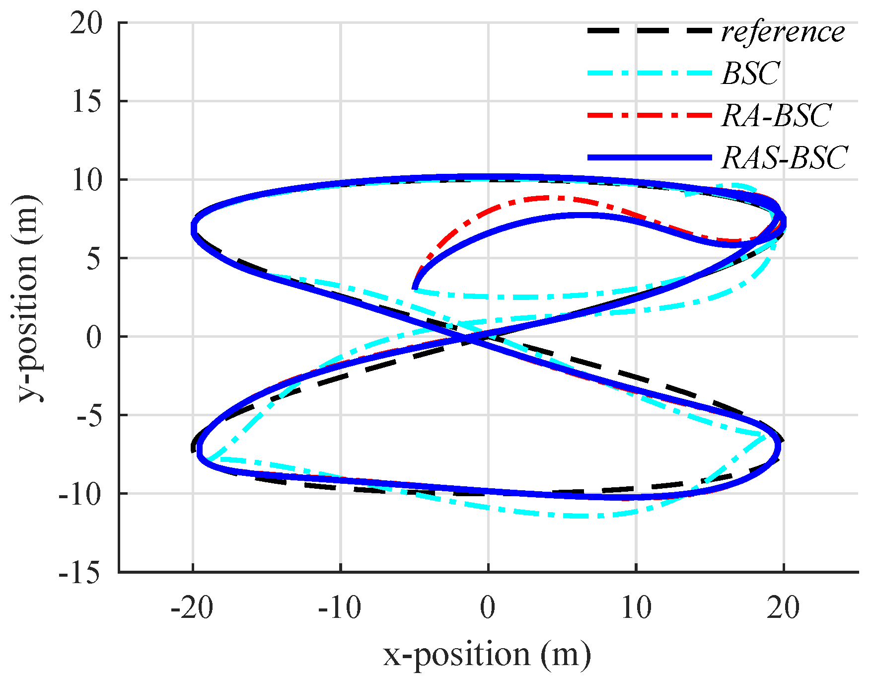
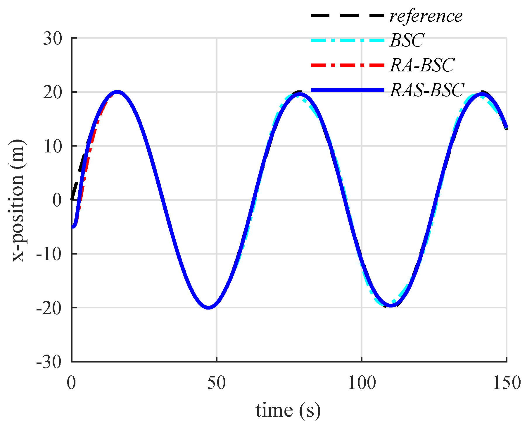
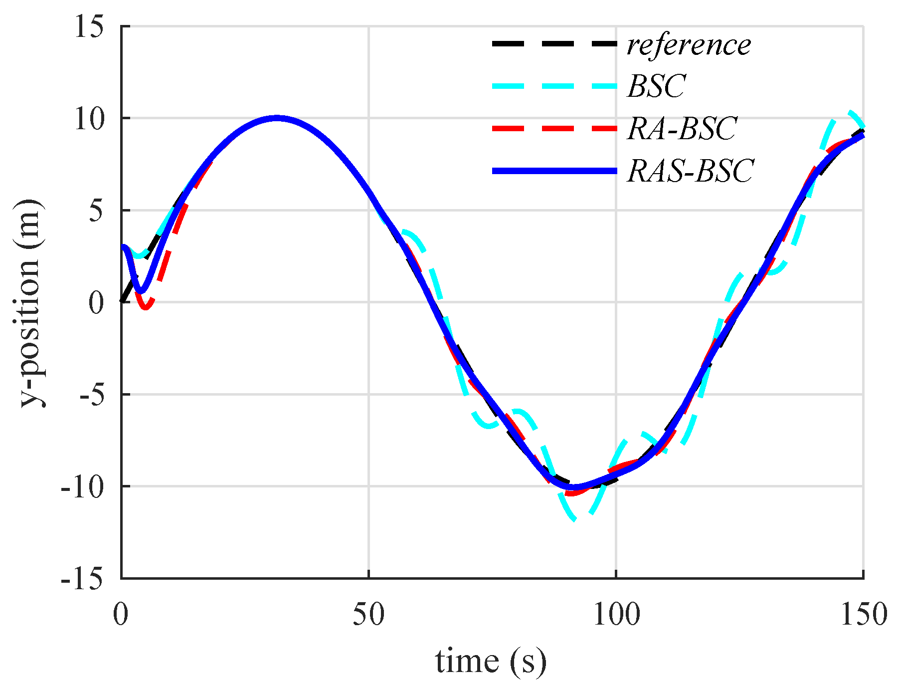
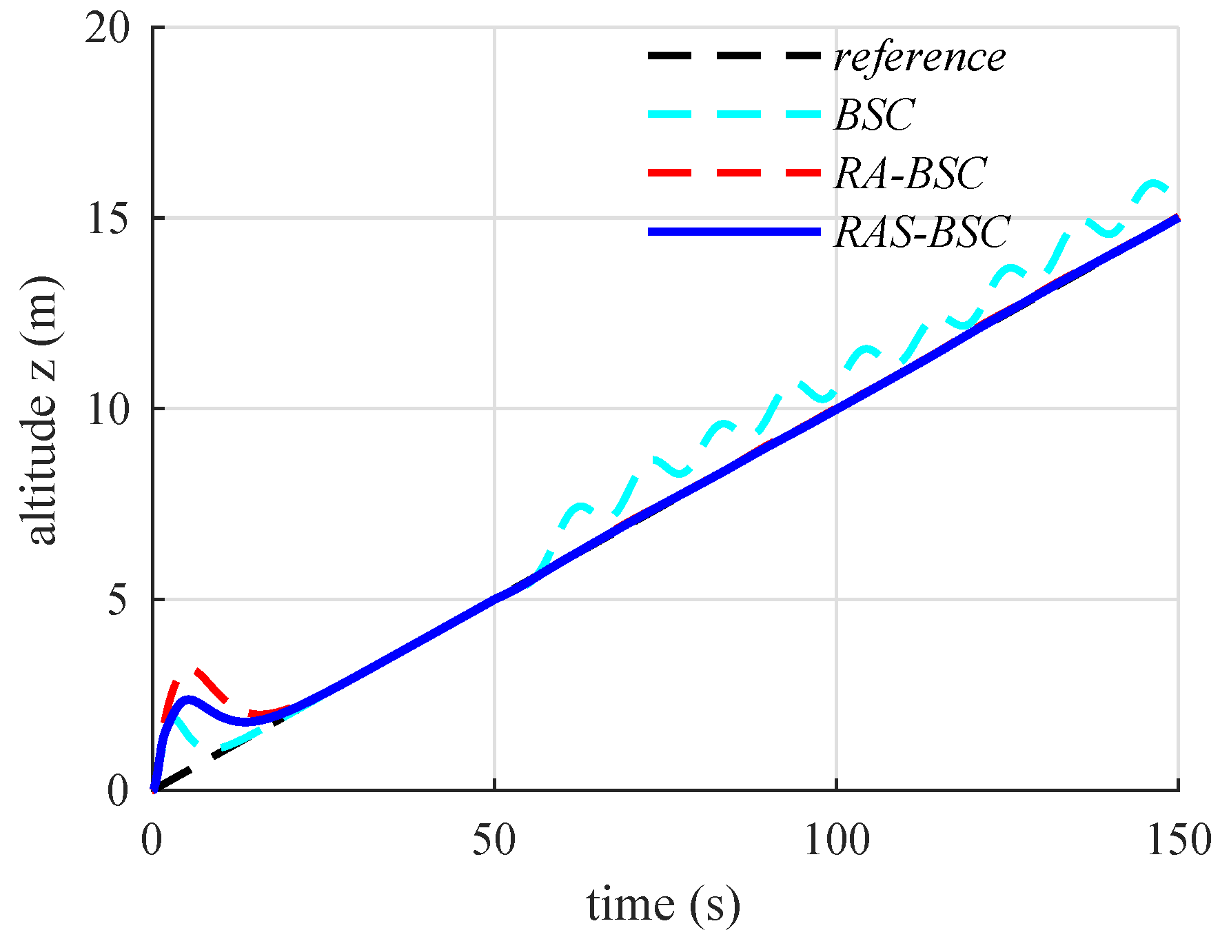
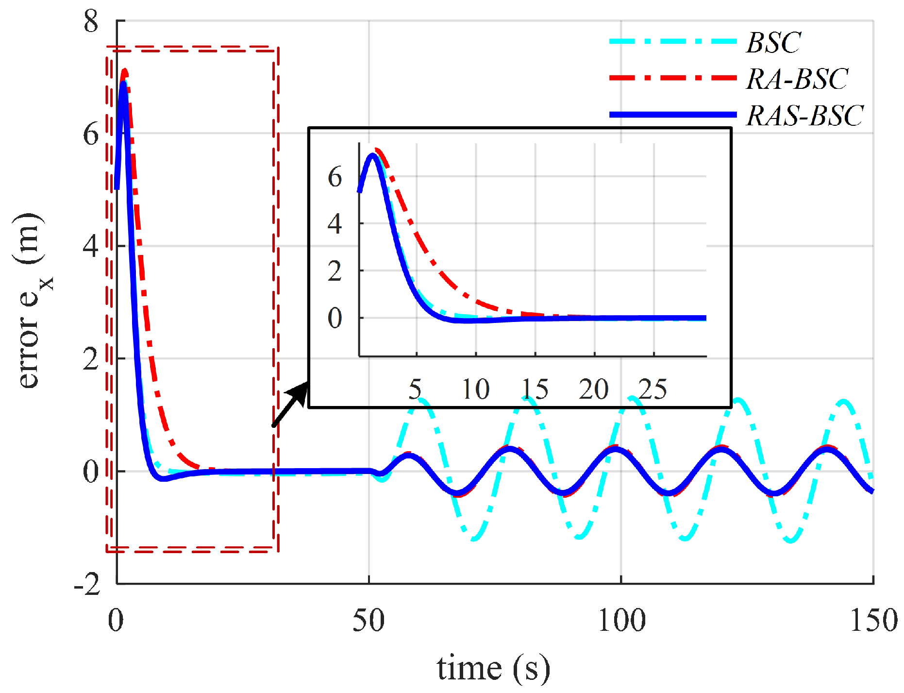
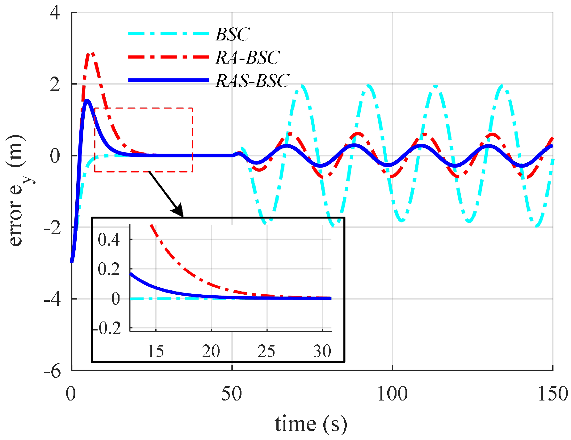
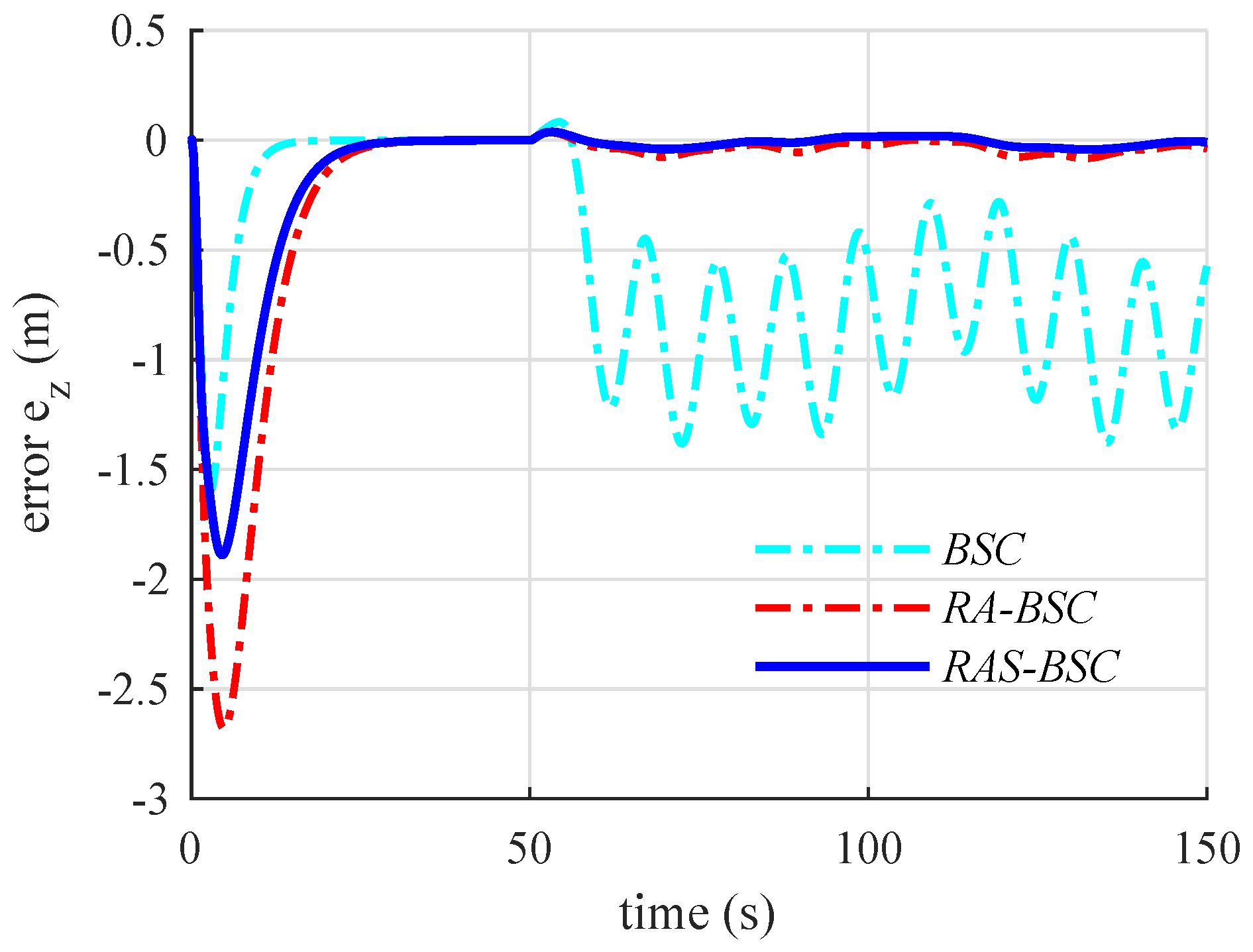
6.2. Simulation Results and Discussions

In the presence of both parameterized uncertainties and external disturbances our new controller is expected to perform similarly to the RA-BSC approach as long as the control input is not saturated. If saturation does occur, our controller should exhibit a superior performance compared to both BSC and RA-BSC. To highlight the effectiveness of our proposed RAS-BSC, the simulation was carried out in two stages: trajectory tracking control in (i) the absence and (ii) the presence of lumped disturbances. For comparison, we also simulated the performance of the BSC and RA-BSC prescribing the same flight conditions.
The first stage covers the time period from t = 0 to t = 50 s. At t = 0 s, the vehicle is initialized and then takes off from the initial position. All three controllers are generally able to drive the quadrotor to the trajectory reference (Figure 2, Figure 3, Figure 4, Figure 5, Figure 6, Figure 7, Figure 8 and Figure 9) and stabilize the vehicle’s attitude (Figure 10, Figure 11 and Figure 12) within a few seconds after taking off. However, all control signals (Figure 13, Figure 14, Figure 15 and Figure 16) reach different saturation values causing significant differences between the three controllers in their convergence times (Table 3). For the BSC, it is ~9 s for x - position, 14 s for y-position, 23 s for z-position, and 6 for heading angle. For the RA-BSC, it is 15 s, 20 s, 35 s, and 9 for x-, y-, z-position, and heading angle, respectively. Whereas with our new algorithm, it is ~9 s, 19 s, 28 s, and 6 , respectively, for the x-, y-, z-position, and heading angle. The slow RA-BSC response time can impose several limitations and pose real dangers in real-world applications, e.g., loss of tracking targets, agent collision in multi-agent systems, breaking a precision landing function, etc.
Here, we can make two main observations: (1) although the RA-BSC converges significantly slower than our new RAS-BSC controller in the presence of control input saturation (first flight stage), the convergence times become much more similar when the control input is not saturated (second flight stage), and (2) although the BSC converges quickly and delivers an acceptable performance in the absence of external disturbances (first flight stage), its tracking mission deteriorates considerably once the external disturbances are applied (second flight stage).
During the second stage (from t = 50 s to t = 150 s), the lumped disturbances are applied to the simulation. As a result, and despite having shown a faster initial response (in the first flight stage) than both RA-BSC and RAS-BSC, the BSC tracking performance deteriorates dramatically once the disturbances influence the system (Figure 2, Figure 3, Figure 4, Figure 5, Figure 6, Figure 7, Figure 8, Figure 9, Figure 10, Figure 11 and Figure 12) and the position tracking error performance exhibits large peak-to-peak amplitudes of oscillation (Table 4). Furthermore, the BSC altitude oscillation remains at a high frequency and never converges to zero (Figure 9). During this stage, the control signals u 1 , u 2 , and u 3 are not saturated (Figure 13, Figure 14 and Figure 15), and, as expected, the position tracking error performance is nearly identical for the RA-BSC and our RAS-BSC. For the RA-BSC, it is, respectively, 0.6 m, 0.7 m, and 0.05 m for the x-, y-, and z-position. Meanwhile, for our new controller, it is 0.6 m, 0.55 m, and 0.05 m for the x-, y-, and z-position, respectively. Furthermore, during this second stage, the control signal u 4 becomes saturated (Figure 16), resulting in a considerable degradation of the RA-BSC heading angle tracking performance (Figure 12 and Table 4) with a peak-to-peak oscillation amplitude of 2.4 , whereas it is only 0.8 for our controller. The numerical simulation results also show that the saturation amounts corresponding to the virtual control signals F and U 2 are all bounded (Figure 17), verifying the reasonability of the saturation assumptions made in Section 4, i.e., Δ F υ 1 and Δ U 2 υ 2 .
In summary, our new controller clearly outperforms the other backstepping-based controllers, despite either parameterized uncertainty in combination with external disturbances or control input saturation. The way our new controller exhibits the performance promises a robust and rapid response, even when the vehicle is flying in disturbance-rich environments and in the presence of control input saturation and sensor faults. This significantly extends the range of applications and environments in which UAVs can be deployed, especially if these applications require high stability, rapid response times, and high accuracy, e.g., for moving obstacle avoidance, precision landing on moving platforms, autonomous delivery to difficult (e.g., narrowed) areas, etc.

7. Conclusions

This paper presented a new robust backstepping tracking control for a quadrotor with input saturation. Using only position and attitude measurements, an ESO was devised to supply estimates of the vehicle’s velocity, angular rate, and lumped disturbances. Taking into account the lumped disturbances and control input saturation, we designed an ESO-based backstepping tracking controller and demonstrated the stability of the closed-loop system through Lyapunov theory. The numerical simulation results clearly demonstrated that our new controller exhibits a significantly improved TTC performance in comparison to existing backstepping-based approaches. Our proposed controller is not only robust and capable to adapt to uncertainties and disturbances but it also maintains rapid response times despite control input saturation. These properties guarantee superior trajectory tracking control performance of the investigated quadrotor and promise a broad range of applications in other system classes. Our future work will be directed to designing a controller (using our RAS-BSC approach) to achieve a precision landing of a quadrotor on a moving platform, which requires superior control performance in disturbance-rich environments.

Author Contributions

Conceptualization, N.X.-M.; methodology, N.X.-M.; software, N.X.-M.; validation, N.X.-M.; formal analysis, N.X.-M.; investigation, N.X.-M.; resources, N.X.-M.; data curation, N.X.-M.; writing—original draft preparation, N.X.-M.; writing—review and editing, N.X.-M. and S.K.H.; visualization, N.X.-M.; supervision, S.K.H.; project administration, S.K.H.; funding acquisition, S.K.H.

Funding

This research received no external funding.

Acknowledgments

This research was supported by the Competency Development Program for Industry Specialists of the Korean Ministry of Trade, Industry and Energy (MOTIE), operated by Korea Institute for Advancement of Technology (KIAT) (No. N0002431) and the MSIT (Ministry of Science and ICT), Korea, under the ITRC (Information Technology Research Center) support program (IITP-2018-2019-0-01423) supervised by the IITP (Institute for Information and Communications Technology Promotion).

Conflicts of Interest

The authors declare no conflicts of interest.

References

  1. Bashi, O.I.D.; Hasan, W.Z.W.; Azis, N.; Shafie, S.; Wagatsuma, H. Unmanned aerial vehicle quadcopter: A review. J. Comput. Theor. Nanosci. 2016, 38, 529–554. [Google Scholar] [CrossRef]
  2. Özbek, N.S.; Önkol, M.; Efe, M.Ö. Feedback control strategies for quadrotor-type aerial robots: A survey. Trans. Inst. Meas. Control 2017, 14, 5663–5675. [Google Scholar] [CrossRef]
  3. Lee, H.; Kim, H.J. Trajectory tracking control of multirotors from modeling to experiments: A survey. Int. J. Control Autom. Syst. 2017, 15, 281–292. [Google Scholar] [CrossRef]
  4. Mung, N.X.; Hong, S.K. A Multicopter ground testbed for the evaluation of attitude and position controller. Int. J. Eng. Technol. 2018, 7, 65–73. [Google Scholar]
  5. Dong, X.; Zhou, Y.; Ren, Z.; Zhong, Y. Time-varying formation control for unmanned aerial vehicles with switching interaction topologies. Control Eng. Pract. 2016, 46, 26–36. [Google Scholar] [CrossRef]
  6. Thanh, H.L.N.N.; Hong, S.K. Quadcopter Robust Adaptive Second Order Sliding Mode Control Based on PID Sliding Surface. IEEE Access 2018, 6, 2169–3536. [Google Scholar]
  7. Kendoul, F. Nonlinear hierarchical flight controller for unmanned rotorcraft: Design, stability, and experiments. J. Guid. Control Dyn. 2009, 32, 1954–1958. [Google Scholar] [CrossRef]
  8. Zuo, Z.Y. Trajectory tracking control design with command-filtered compensation for a quadrotor. IET Control Theory Appl. 2010, 4, 2343–2355. [Google Scholar] [CrossRef]
  9. Nguyen, A.T.; Xuan-Mung, N. Quadcopter Adaptive Trajectory Tracking Control: A New Approach via Backstepping Technique. Appl. Sci. 2019, 9, 3873. [Google Scholar] [CrossRef]
  10. Liu, H.; Zhao, W.; Hong, S.; Lewis, F.L.; Yu, Y. Robust backstepping-based trajectory tracking control for quadrotors with time delays. IET Control Theory Appl. 2019, 13, 1945–1954. [Google Scholar] [CrossRef]
  11. Gao, H.; Chen, T. Network-based H∞ output tracking control. IEEE Trans. Autom. Control 2008, 53, 655–670. [Google Scholar] [CrossRef]
  12. Raffo, G.V.; Ortega, M.G.; Rubio, F.R. An integral predictive/nonlinear H infinity control structure for a quadrotor helicopter. Automatica 2010, 46, 29–39. [Google Scholar] [CrossRef]
  13. Xiong, J.J.; Zheng, E.H. Position and attitude tracking control for a quadrotor UAV. ISA Trans. 2014, 53, 1350–1356. [Google Scholar] [CrossRef] [PubMed]
  14. Shah, M.Z.; Samar, R.; Bhatti, A.I. Lateral track control of UAVs using the sliding mode approach: From design to flight testing. Trans. Inst. Meas. Control 2015, 37, 457–474. [Google Scholar] [CrossRef]
  15. Li, Z.; Deng, J.; Lu, R.; Xu, Y.; Bai, J.; Su, C.Y. Trajectory-tracking control of mobile robot systems incorporating neural-dynamic optimized model predictive approach. IEEE Trans. Syst. Man Cybern. Syst. 2016, 46, 740–749. [Google Scholar] [CrossRef]
  16. Nascimento, T.P.; Saska, M. Position and attitude control of multi-rotor aerial vehicles: A survey. Annu. Rev. Control 2019, 48, 129–146. [Google Scholar] [CrossRef]
  17. Tahir, A.; Böling, J.; Haghbayan, M.H.; Toivonen, H.T.; Plosila, J. Swarms of Unmanned Aerial Vehicles—A Survey. IEEE J. Ind. Inf. Integr. 2019, 16, 100106. [Google Scholar] [CrossRef]
  18. Carrillo, L.R.G.; Vamvoudakis, K.G. Deep-Learning Tracking for Autonomous Flying Systems Under Adversarial Inputs. In IEEE Transactions on Aerospace and Electronic Systems; IEEE: Piscataway, NJ, USA, 2019. [Google Scholar]
  19. Jafari, M.; Xu, H.; Carrillo, L.R.G. A neurobiologically-inspired intelligent trajectory tracking control for unmanned aircraft systems with uncertain system dynamics and disturbance. Trans. Inst. Meas. Control 2019, 41, 417–432. [Google Scholar] [CrossRef]
  20. Jafari, M.; Xu, H. Intelligent control for unmanned aerial systems with system uncertainties and disturbances using artificial neural network. Drones 2018, 2, 30. [Google Scholar]
  21. Wang, N.; Su, S.F.; Han, M.; Chen, W.H. Backpropagating constraints-based trajectory tracking control of a quadrotor with constrained actuator dynamics and complex unknowns. IEEE Trans. Syst. Man, Cybern. Syst. 2018, 49, 1322–1337. [Google Scholar] [CrossRef]
  22. Chen, F.; Lei, W.; Zhang, K.; Tao, G.; Jang, B. A novel nonlinear resilient control for a quadrotor UAV via backstepping control and nonlinear disturbance observer. Nonlinear Dyn. 2016, 85, 1281–1295. [Google Scholar] [CrossRef]
  23. Yacef, F.; Bouhail, O.; Hamerlain, M.; Rizoug, N. Observer-based adaptive fuzzy backstepping tracking control of quadrotor unmanned aerial vehicle powered by li-ion battery. J. Intell. Robot. Syst. 2016, 84, 179–197. [Google Scholar] [CrossRef]
  24. Fang, X.; Wu, A.G.; Shang, Y.J.; Dong, N. A novel sliding mode controller for small-scale unmanned helicopters with mismatched disturbance. Nonlinear Dyn. 2016, 83, 1053–1068. [Google Scholar] [CrossRef]
  25. Yacef, F.; Bouhail, O.; Hamerlain, M.; Rizoug, N. Adaptive RBFNN/integral sliding mode control for a quadrotor aircraft. Neurocomputing 2016, 216, 126–134. [Google Scholar]
  26. Ahmed, N.; Chen, M. Sliding mode control for quadrotor with disturbance observer. Adv. Mech. Eng. 2018, 10, 1–16. [Google Scholar] [CrossRef]
  27. Rodr-guez-Mata, A.E.; Flores, G.; Mart-nez-Vásquez, A.H.; Mora-Felix, Z.D.; Castro-Linares, R.; Amabilis-Sosa, L.E. Discontinuous High-Gain Observer in a Robust Control UAV Quadrotor: Real-Time Application for Watershed Monitoring. Math. Probl. Eng. 2018, 2018, 4940360. [Google Scholar]
  28. Chen, M.; Xiong, S.; Wu, Q. Tracking Flight Control of Quadrotor Based on Disturbance Observer. In IEEE Transactions on Systems, Man, and Cybernetics: Systems; IEEE: Piscataway, NJ, USA, 2019; pp. 2168–2216. [Google Scholar]
  29. Shao, X.; Liu, J.; Cao, H.; Shen, C.; Wang, H. Robust dynamic surface trajectory tracking control for a quadrotor UAV via extended state observer. Int. J. Robust Nonlinear Control 2018, 28, 2700–2719. [Google Scholar] [CrossRef]
  30. Liu, H.; Li, D.; Yu, Y.; Zhong, Y. Robust trajectory tracking control of uncertain quadrotors without linear velocity measurements. IET Control Theory Appl. 2015, 9, 1746–1754. [Google Scholar] [CrossRef]
  31. Ma, D.; Xia, Y.; Li, T.; Chang, K. Active disturbance rejection and predictive control strategy for a quadrotor helicopter. IET Control Theory Appl. 2016, 10, 2213–2222. [Google Scholar] [CrossRef]
  32. Zou, Y. Trajectory tracking controller for quadrotors without velocity and angular velocity measurements. IET Control Theory Appl. 2017, 11, 101–109. [Google Scholar] [CrossRef]
  33. Tian, B.; Lu, H.; Zuo, Z.; Zong, Q.; Zhang, Y. Multivariable finite-time output feedback trajectory tracking control of quadrotor helicopters. Int. J. Robust Nonlinear Control 2017, 28, 281–295. [Google Scholar] [CrossRef]
  34. Shao, X.; Liu, J.; Wang, H. Robust backstepping output feedback trajectory tracking for quadrotors via extended state observer and sigmoid tracking differentiator. Mech. Syst. Signal Process. 2018, 104, 631–647. [Google Scholar] [CrossRef]
  35. He, M.; He, J. Extended State Observer-Based Robust Backstepping Sliding Mode Control for a Small-Size Helicopter. IEEE Access 2018, 6, 33480–33488. [Google Scholar] [CrossRef]
  36. Zarovy, S.; Costello, M. Extended state observer for helicopter mass and center-of-gravity estimation. J. Aircr. 2015, 52, 1939–1949. [Google Scholar] [CrossRef]
  37. Koria, D.K.; Kolhe, J.P.; Talole, S.E. Extended state observer based robust control of wing rock motion. Aerosp. Sci. Technol. 2014, 33, 107–117. [Google Scholar] [CrossRef]
  38. Wang, Q.; Ran, M.; Dong, C. Robust partial integrated guidance and control for missiles via extended state observer. ISA Trans. 2016, 65, 27–36. [Google Scholar] [CrossRef]
  39. Shao, X.; Wang, H. Back-stepping active disturbance rejection control design for integrated missile guidance and control system via reduced-order ESO. ISA Trans. 2015, 57, 10–22. [Google Scholar]
  40. Wei, Q.; Chen, M.; Wu, Q. Backstepping-based attitude control for a quadrotor UAV with input saturation and attitude constraints. Control Theory Appl. 2018, 10, 1361–1369. [Google Scholar]
  41. Cao, N.; Lynch, A.F. Inner—Outer Loop Control for Quadrotor UAVs With Input and State Constraints. IEEE Trans. Control Syst. Technol. 2016, 24, 1797–1804. [Google Scholar] [CrossRef]
  42. Faessler, M.; Falanga, D.; Scaramuzza, D. Thrust Mixing, Saturation, and Body-Rate Control for Accurate Aggressive Quadrotor Flight. IEEE Robot. Autom. Lett. 2017, 2, 476–482. [Google Scholar] [CrossRef]
  43. Li, S.; Wang, Y.; Tan, J. Adaptive and robust control of quadrotor aircrafts with input saturation. Nonlinear Dyn. 2017, 89, 255–265. [Google Scholar] [CrossRef]
  44. Jiang, T.; Lin, D.; Song, T. Finite-Time Backstepping Control for Quadrotors With Disturbances and Input Constraints. IEEE Access 2018, 6, 62037–62049. [Google Scholar] [CrossRef]
  45. Wang, X.; Su, X.; Sun, L. Disturbance observer-based singularity-free trajectory tracking control of uncertain quadrotors with input saturation. In Proceedings of the 2018 Chinese Control And Decision Conference (CCDC), Shenyang, China, 9–11 June 2018; pp. 5780–5785. [Google Scholar]
  46. Huang, Y.; Zheng, Z.; Sun, L.; Zhu, M. Saturated adaptive sliding mode control for autonomous vessel landing of a quadrotor. IET Control Theory Appl. 2018, 12, 1830–1842. [Google Scholar] [CrossRef]
  47. Liu, Z.; Liu, W.; Gong, X.; Wu, J. Simplified Attitude Determination Algorithm Using Accelerometer and Magnetometer with Extremely Low Execution Time. J. Sens. 2018, 2018, 8787236. [Google Scholar] [CrossRef] [Green Version]
  48. Celis, R.; Cadarso, L. Attitude Determination Algorithms through Accelerometers, GNSS Sensors, and Gravity Vector Estimator. Int. J. Aerosp. Eng. 2018, 2018, 5394057. [Google Scholar] [CrossRef] [Green Version]
  49. Tan, C.K.; Wang, J.; Paw, Y.C.; Ng, T.Y. Tracking of a moving ground target by a quadrotor using a backstepping approach based on a full state cascaded dynamics. Appl. Soft Comput. 2017, 47, 47–62. [Google Scholar] [CrossRef]
  50. Mung, N.X.; Hong, S.K. Improved Altitude Control Algorithm for Quadcopter Unmanned Aerial Vehicles. Appl. Sci. 2019, 9, 2122. [Google Scholar] [CrossRef] [Green Version]
  51. Mung, N.X.; Hong, S.K. Robust Adaptive Formation Control of Quadcopters based on a Leader-Follower Approach. Int. J. Adv. Robot. Syst. 2019, 16. [Google Scholar] [CrossRef] [Green Version]
  52. Khalil, H.K. Nonlinear Systems, 3rd ed.; Prentice Hall: Upper Saddle River, NJ, USA, 2002. [Google Scholar]
  53. Guo, Q.; Zhang, Y.; Celler, B.G.; Su, S.W. Back-stepping control of electro-hydraulic system based on Extended-state-observer with plant dynamics largely unknown. IEEE Trans. Ind. Electron. 2016, 63, 6909–6920. [Google Scholar] [CrossRef]
  54. Song, B.; Hedrick, J.K. Dynamic Surface Control of Uncertain Nonlinear System; Springer-Verlag London Limited: London, UK, 2011; pp. 19–55. [Google Scholar]
  55. Flame Wheel ARF Kit. Available online: https://www.dji.com/kr/flame-wheel-arf/spec (accessed on 1 October 2019).
  56. DJI E305. Available online: http://www.dji.com/product/e305 (accessed on 1 October 2019).
Figure 1. Quadrotor configuration.
Applsci 09 05184 g001
Figure 2. Three-dimensional view of the trajectory tracking performance of the three controllers.
Applsci 09 05184 g002
Figure 3. Two-dimensional view of the trajectory tracking performance of the three controllers.
Applsci 09 05184 g003
Figure 4. Comparing the trajectory tracking performance of the three controllers along the x-direction.
Applsci 09 05184 g004
Figure 5. Comparing the trajectory tracking performance of the three controllers along the y-direction.
Applsci 09 05184 g005
Figure 6. Comparing the trajectory tracking performance of the three controllers along the z-direction.
Applsci 09 05184 g006
Figure 7. Comparison of x-position tracking error performance between our new controller (RAS-BSC) and existing controllers.
Applsci 09 05184 g007
Figure 8. Comparison of y-position tracking error performance between our new controller (RAS-BSC) and existing controllers.
Applsci 09 05184 g008
Figure 9. Comparison of altitude tracking error performance between our new controller (RAS-BSC) and existing controllers.
Applsci 09 05184 g009
Figure 10. Comparison of roll attitude performance between our new controller (RAS-BSC) and existing controllers.
Applsci 09 05184 g010
Figure 11. Comparison of pitch attitude performance between our new controller (RAS-BSC) and existing controllers.
Applsci 09 05184 g011
Figure 12. Comparison of yaw attitude performance between our new controller (RAS-BSC) and existing controllers.
Applsci 09 05184 g012
Figure 13. Comparison of control signal u 1 between our new controller (RAS-BSC) and existing controllers.
Applsci 09 05184 g013
Figure 14. Comparison of control signal u 2 between our new controller (RAS-BSC) and existing controllers.
Applsci 09 05184 g014
Figure 15. Comparison of control signal u 3 between our new controller (RAS-BSC) and existing controllers.
Applsci 09 05184 g015
Figure 16. Comparison of control signal u 4 between our new controller (RAS-BSC) and existing controllers.
Applsci 09 05184 g016
Figure 17. The magnitude of the saturation amounts, Δ F and Δ U 2 , are all bounded, which verifies the reasonability of the saturation assumptions Δ F υ 1 and Δ U 2 υ 2 .
Applsci 09 05184 g017
Table 1. System’s nominal parameters used in the simulation.
SymbolValueUnit
m 2.0 kg
J 1 0.0121 kg·m 2
J 2 0.0119 kg·m 2
J 3 0.0223 kg·m 2
l 0.225 m
c d 0.05
g 9.81 m/s 2
Λ 1 diag [ 0.01 , 0.01 , 0.01 ]
Λ 2 diag [ 0.012 , 0.012 , 0.012 ]
u 1 max 30N
u 2 max 1.8Nm
u 3 max 1.8Nm
u 4 max 3Nm
Table 2. Trajectory reference, desired heading angle, initial conditions, and controller gains used in the simulation.
SymbolValue and UnitDescription
P d [20sin( 0.1 t), 10sin( 0.05 t), 0.1 t] mTrajectory reference
ψ d 0 Desired heading angle
P 0 [ - 5 , 3 , 0 ] mInitial position
P ˙ 0 [ 0 , 0 , 0 ] m/sInitial velocity
Θ 0 [ 0 , 0 , 6 ] Initial attitude
Θ ˙ 0 [ 0 , 0 , 0 ] /sInitial angular velocity
ω 1 , ω 2 5 , 35 ESO’s bandwidth
k 1 diag[ 0.8 , 0.8 , 0.27 ]Controller gains
k 2 diag[ 0.38 , 0.38 , 0.38 ]Controller gains
k 3 diag[ 1.05 , 1.05 , 1.75 ]Controller gains
k 4 diag[ 2.0 , 2.0 , 0.8 ]Controller gains
k 5 diag[ 1.0 , 1.0 , 0.8 ]Controller gains
k 6 diag[ 4.0 , 4.0 , 5.0 ]Controller gains
c j 1Controller gains
τ 2 , τ 5 0.01LPF’s parameters
Table 3. Comparison of converging time during the first flight stage (in the absence of external disturbances).
Controllerx-Positiony-Positionz-PositionHeading Angle
BSC9 s14 s23 s6 s
RA-BSC15 s24 s35 s9 s
RAS-BSC9 s19 s28 s6 s
Table 4. Comparison of peak-to-peak oscillation amplitude of control performance during the second flight stage (in the presence of external disturbances).
Controllerx-Positiony-Positionz-PositionHeading Angle
BSC 2.9 m 4.5 m 0.7 m 26
RA-BSC 0.6 m 0.7 m 0.05 m 2.4
RAS-BSC 0.6 m 0.55 m 0.05 m 0.8

