5.2. Approach I
The approach will be explained in the case of an undrained clay slope characterised by the spatially variable undrained shear strength .
The mean (i.e.,
) of
for
, based on deterministic finite element analysis (FEA), is found first. Next, using this value of
(e.g.,
kPa for the slope analysed in
Figure 6) and the corresponding values of
and
, the
distribution in the slope is generated (note that, due to the relative positioning of weak and strong zones in the slope, the realised
could be larger or smaller than 1.0). The
values (for the realisation generated in the last step) are then scaled up by progressively larger values of
, and, for each value of
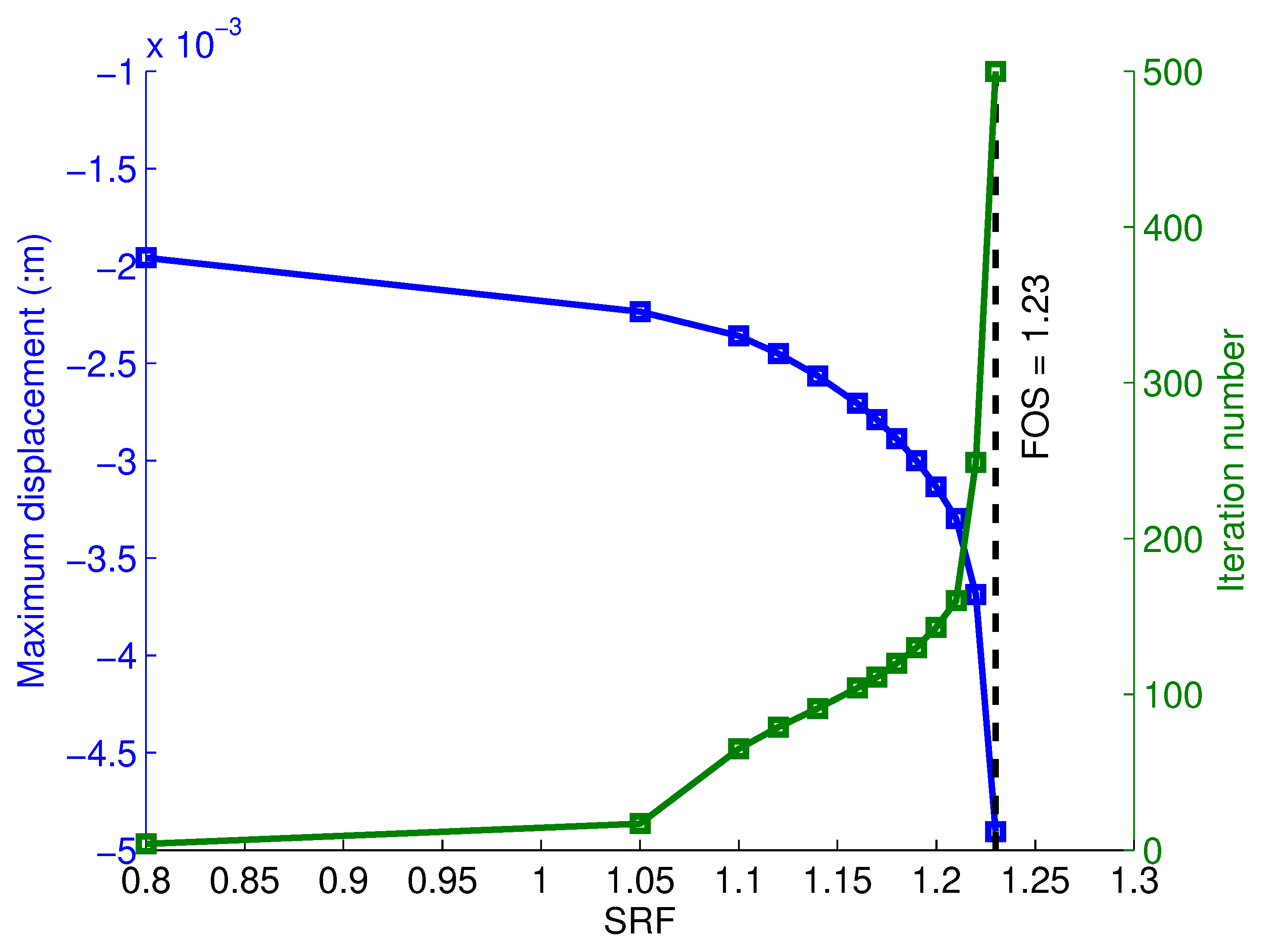
, the slope is analysed to see if it is stable (i.e., the FEA is conducted only for one trial SRF = 1.0, if the plastic iteration count reaches 500, then the slope fails; that is
. The algorithm does not try to find the exact
; it could be any value smaller than 1.0 if the slope failed). By repeating this process for a large number of realisations (
N) while counting the number of failed slopes (
) for each
, the reliability of the slope may be computed for a range of values of
, thereby resulting in a reliability versus
curve.
Note that if the FEA converges within iterations (i.e., less than 500) with a trial SRF = 1.0, then it means that the realised for that realisation must be larger than 1.0 (i.e., an SRF larger than 1.0 is needed to allow the plastic algorithm to hit the 500 iteration ceiling); that is, the slope is stable for that that is used to scale up that realisation.
The pseudocode for approach I is as follows ( is the plastic iteration count):
******************************block 1****************************
10 Initialisation: and input
20 For N realisations (loop i):
30 Generate a slope and shear strength profile () with ;
40 For a series of values of
(e.g., with ) (loop j):
50 Scale up profile by
60 Carry out FEA, let , if , then
70 Output: for each
******************************block 1****************************
or alternatively,
******************************block 2****************************
10 Initialisation: and input
20 For a series of values of
(e.g., with ) (loop j):
30 For N realisations (loop i):
40 Generate a slope and shear strength profile () with ;
50 Scale up profile by
60 Carry out FEA, let , if , then
70 Output: for each
******************************block 2****************************
The algorithm presented in block 2 is not efficient compared to that shown in block 1 as line 30 needs to be regenerated for each considered.
The probability of failure,
, for a given
, is
in which
N is the total number of realisations and
(in which superscript 1 denotes the approach I) is the number of realisations in which slope failure has occurred (i.e.,
).
5.3. Approach II
The (i.e., undrained shear strength) distribution in the slope is generated, based on the statistics (i.e., mean , variance and scales of fluctuation ) of . The factor of safety for each realisation of the slope is then found by scaling down the values of by progressively larger values of strength reduction factor (SRF), until the limiting value of SRF (i.e., the realised ) is obtained. This process is repeated for a large number of realisations, to obtain a distribution of .
The pseudocode for approach II is as follows:
******************************block 3****************************
10 Input statistics corresponding to
20 For N realisations (loop k):
30 Generate a slope and shear strength profile () with ;
40 Carry out FEA using progressively larger SRF, if , then
50 Output: a distribution of
******************************block 3****************************
Note the similarity of block 3 to block 2; block 3 has one input and tries to find the whole distribution of for all realisations, whereas block 2 works on a series values of and does not try to find the exact for all realisations (only to see if it is stable or not).
Now, define a unified factor
as
Note that, for a particular realisation, if is proportional to (or any other value ) by a factor of (or ), the realised is also propotional to (or ) by the same factor. This is because, whether one starts the strength reduction process (to get the realised factor of safety for that realisation) from a high mean shear strength (high ) or a low mean shear strength (low ), in both cases the slope falls down when the mean strength along the failure surface reaches the same critical value (for the same spatial variation of soil properties). For example, if and for a particular realisation (the critical value of strength is then , where is the random cell values along the failure path, generated based on , and f is a function that determines the mean strength along the failure path); then, for the case of , to reach the same critical value, the realised must be . In this case, . For multiple realisations, the same holds.
The probability of failure,
, at a given
, is
in which
N is the total number of realisations and
(in which superscript 2 denotes the approach II) is the number of realisations in which slope failure has occurred (i.e.,
).
The failure is defined as a slope failed at
for any
, e.g.,
. Upon transformation to
(Equation (
6)), the definition of slope failure is preserved by defining
as failure (i.e., when
in Equation (
6),
).
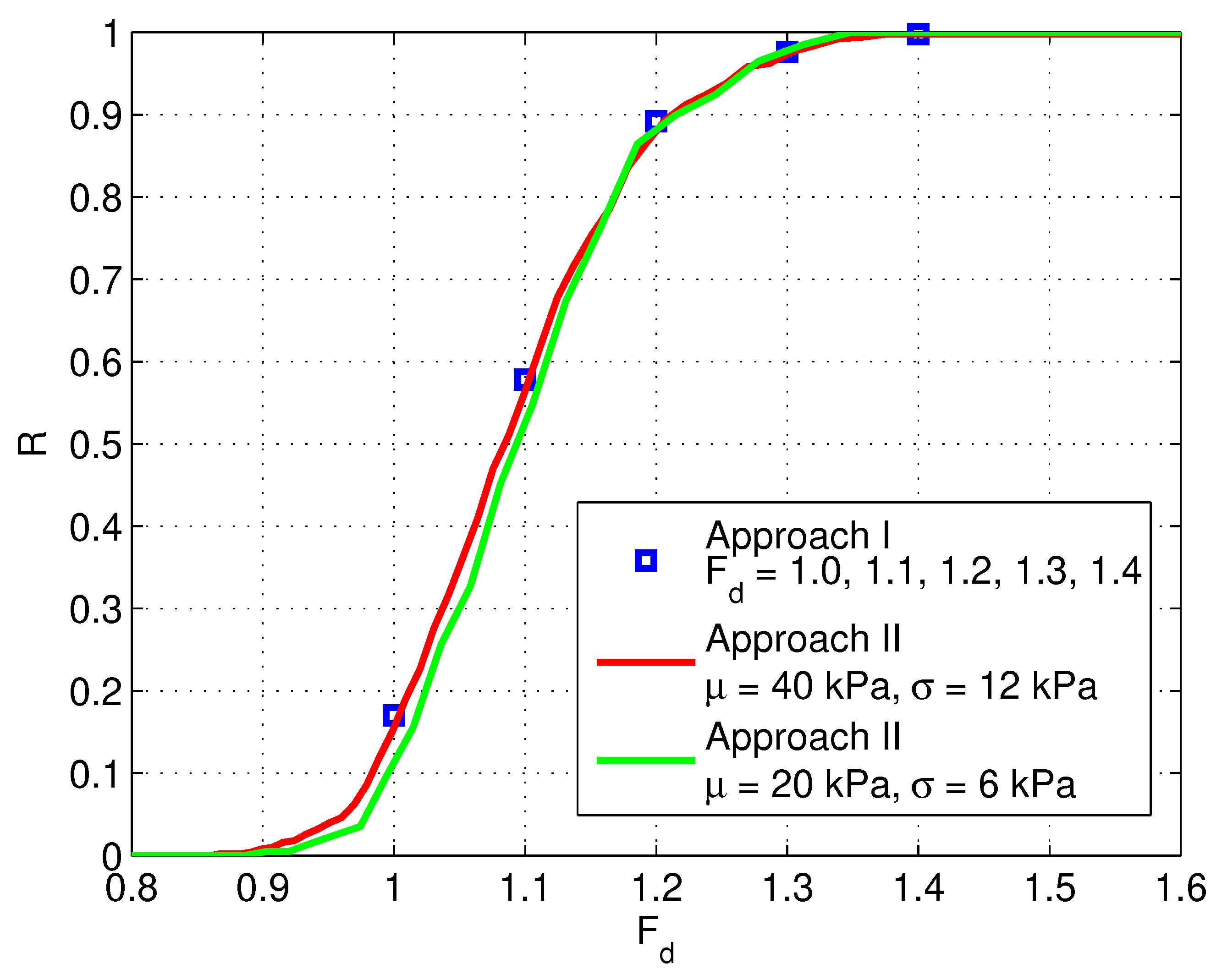
As shown in
Figure 7, an analysis based on
kPa and
kPa (
) gives virtually the same results as the analysis based on
kPa and
kPa (
), where
. The slight difference is due to the different settings (initial FOS, initial FOS step and the three cut values of plastic iteration counts) for the AutoFOS implementation.
Note that it does not matter whether the input statistics are
kPa and
kPa (
) or
kPa and
kPa (
= 1.23). Therefore, for
, the transformed outputs
(the subscript
i denotes “identical”) are the same, based on Equation (
6), if the initial seed for generating the random field is identical (thereby the relative strong and weak spatial distribution of soil properties in the individual realisation of random field is the same for the two cases, only the random field cell values differ by a factor of 2).
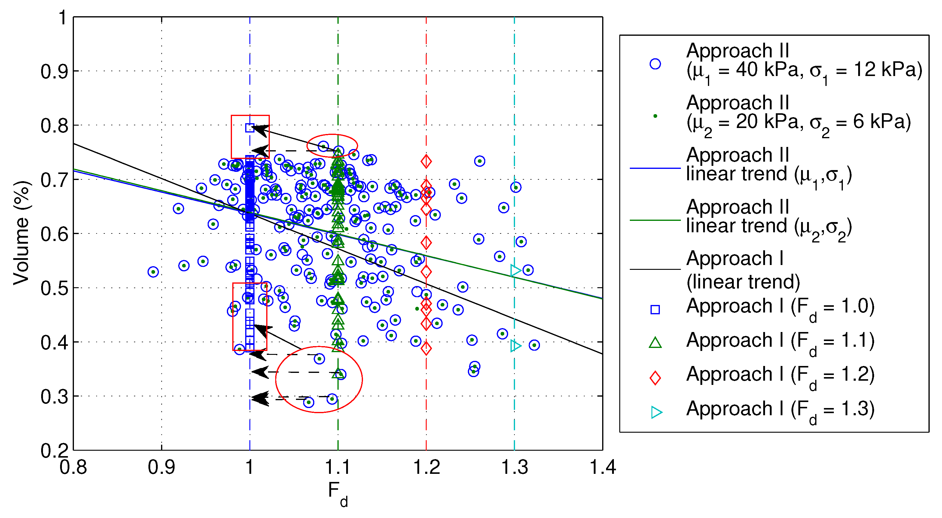
This is clearly shown in
Figure 8, where an analysis based on 40 kPa and 12 kPa gives the same failure volumes as those for an analysis based on 20 kPa and 6 kPa, as indicated by the points sitting in the centre of the circles.
The results of analyses based on Approach I with different sets of inputs (
Table 1) are also shown in
Figure 7. They are in good agreement with the results of Approach II. For each set of input, if the analysis were done in the same way as Approach II to get the whole distribution of
, the fitted curve would be similar to those shown in
Figure 9 (not necessarily the same, because those curves are based on hypothetically generated random numbers).
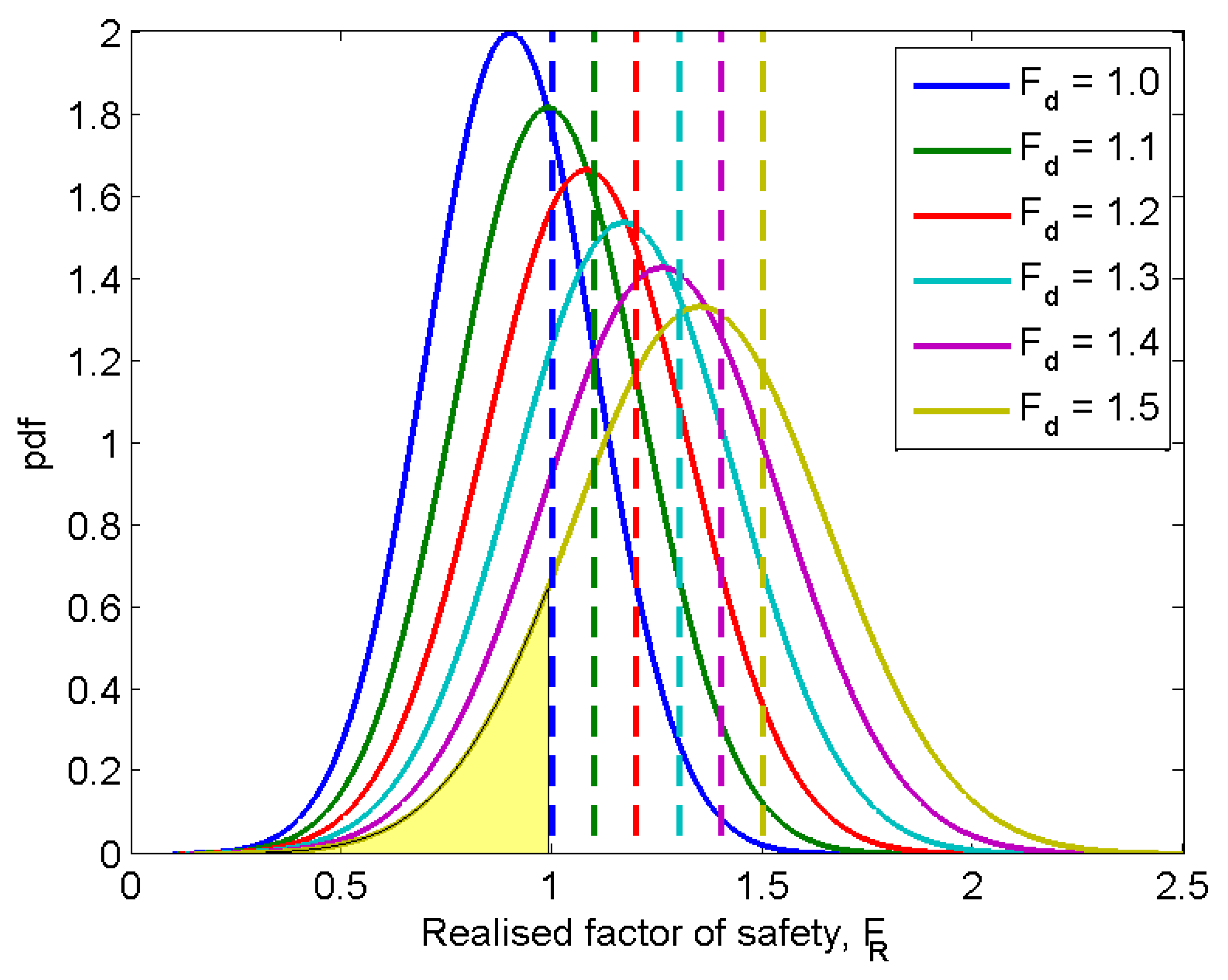
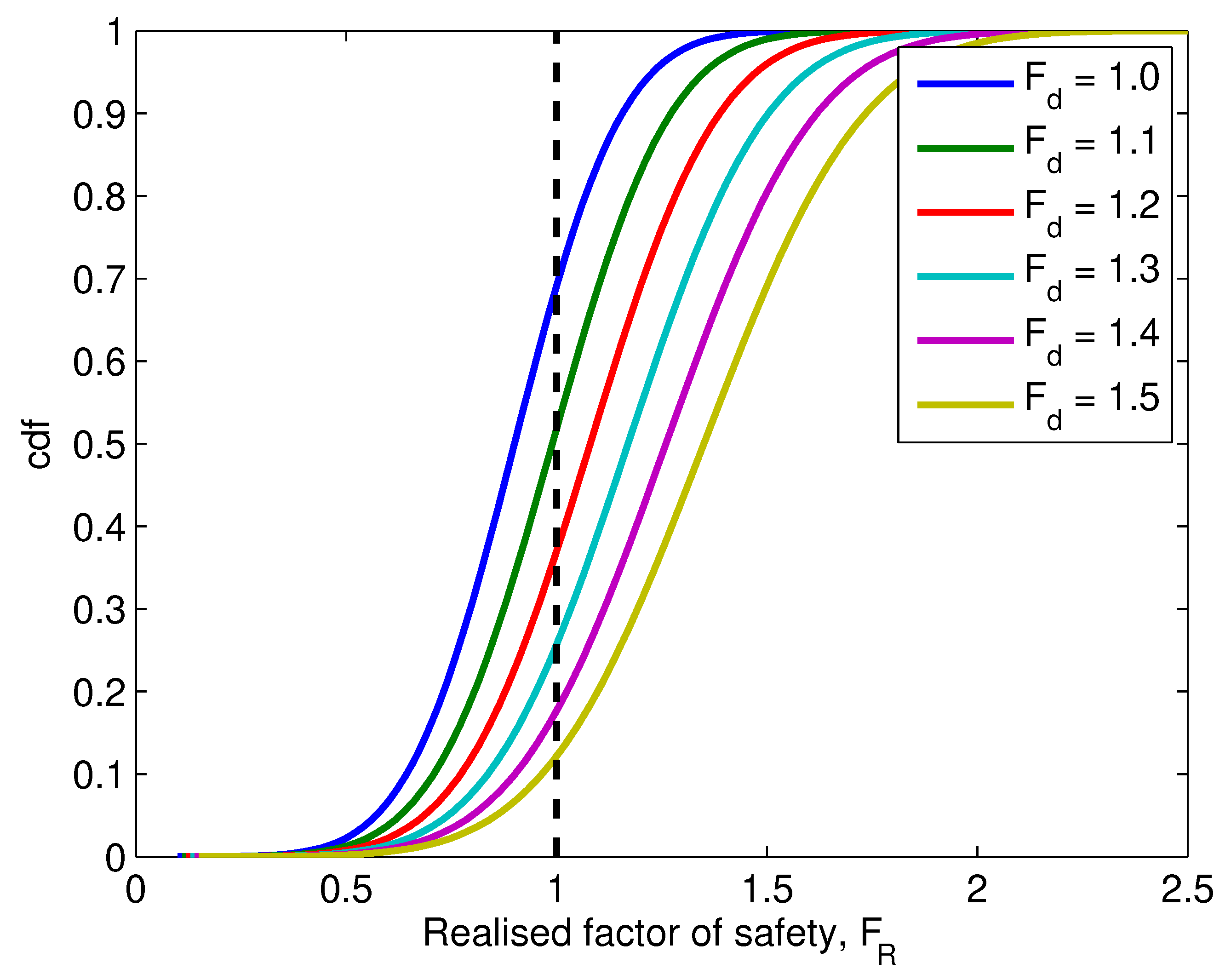
Figure 9 shows the changing of probability of failure as
increases, as represented by the areas under the corresponding pdf curves to the left of 1.0 (the probability of failure can also be read directly from the cdf curves shown in
Figure 10). Those curves represent the fitted curves of the realised
. The curve corresponding to
is hypothetically created based on a mean of 0.9 and a standard deviation of 0.2 (that is,
and
; note that the value of
is assumed here to represent a smaller mean
than
that was observed in a typical RFEM analysis), and those corresponding to 1.1, 1.2, 1.3, 1.4 and 1.5 are created by scaling up the
for
by factors of
,
,
,
and
, respectively (cf. Equation (
6)). By doing so,
and
, for various
, are also scaled up by the same factors. Therefore, the relative position of
and
does not change; this is in accordance with Equation (
6).
5.4. Equivalence and Differences between the Two Approaches
In essence, these two methods are equivalent to each other. Approach II is a unified approach, regardless of the specific input provided that COV is constant. This can be explained by Equation (
6). In fact, once a distribution of
is obtained from a base case, for example,
, the distributions of
for other values (i.e., any value) of
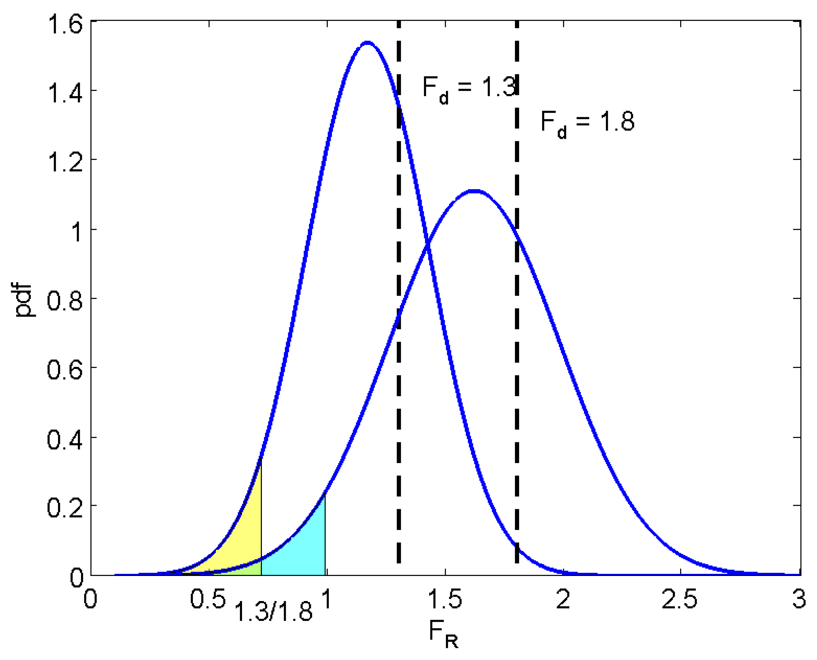
can be inferred. This is shown in
Figure 11. Not only the distribution can be inferred, but also the probability of failure
for any
. As shown in
Figure 11, the shaded area below the pdf to the left side of 1.0, for a given
, is equal to the shaded area below the pdf to the left side of
. The reason behind this lies in the following expression of the cumulative distribution function of a normal distribution,
where
is the error function.
Based on the above equation, and by setting and changing the values of and for any given series of values of (which is proportional to the value of and for the base case ), the reliability versus curve can be obtained; this is essentially Approach I.
The same results can be obtained by only looking at the distribution of
for the base case. That is, in Equation (
8), let
and
be the values based on the base case, and change the value of
to be
. This way, the reliability versus
curve can also be obtained; this is essentially Approach II.
Note that the series of
values can be any prescribed values, for example,
. In a typical RFEM simulation, one can either prescribe a series of
values or by simply taking the values of
from the base case and using them as the series of
values (or take the values of
(Equation (
6)) as the prescribed
).
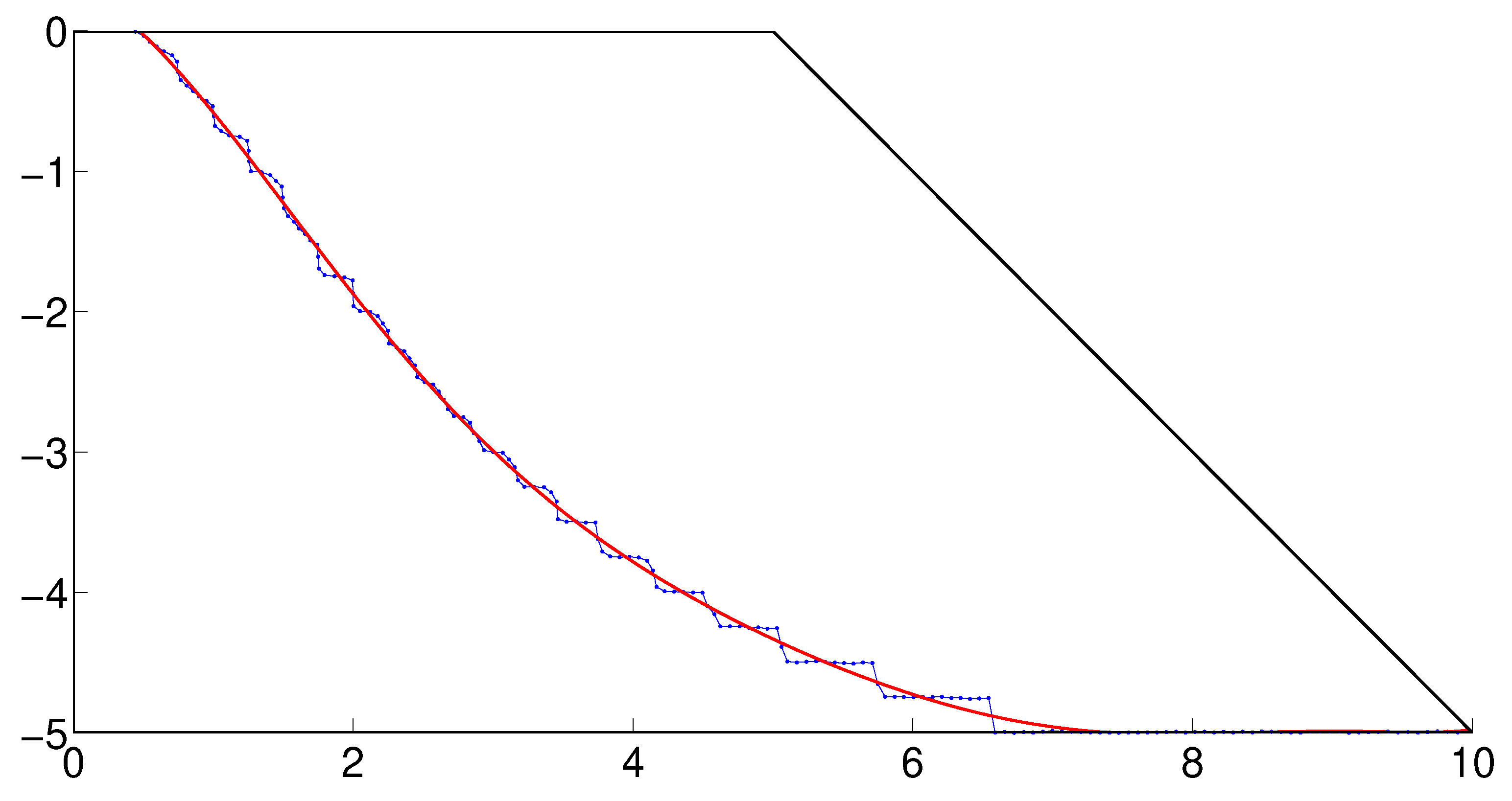
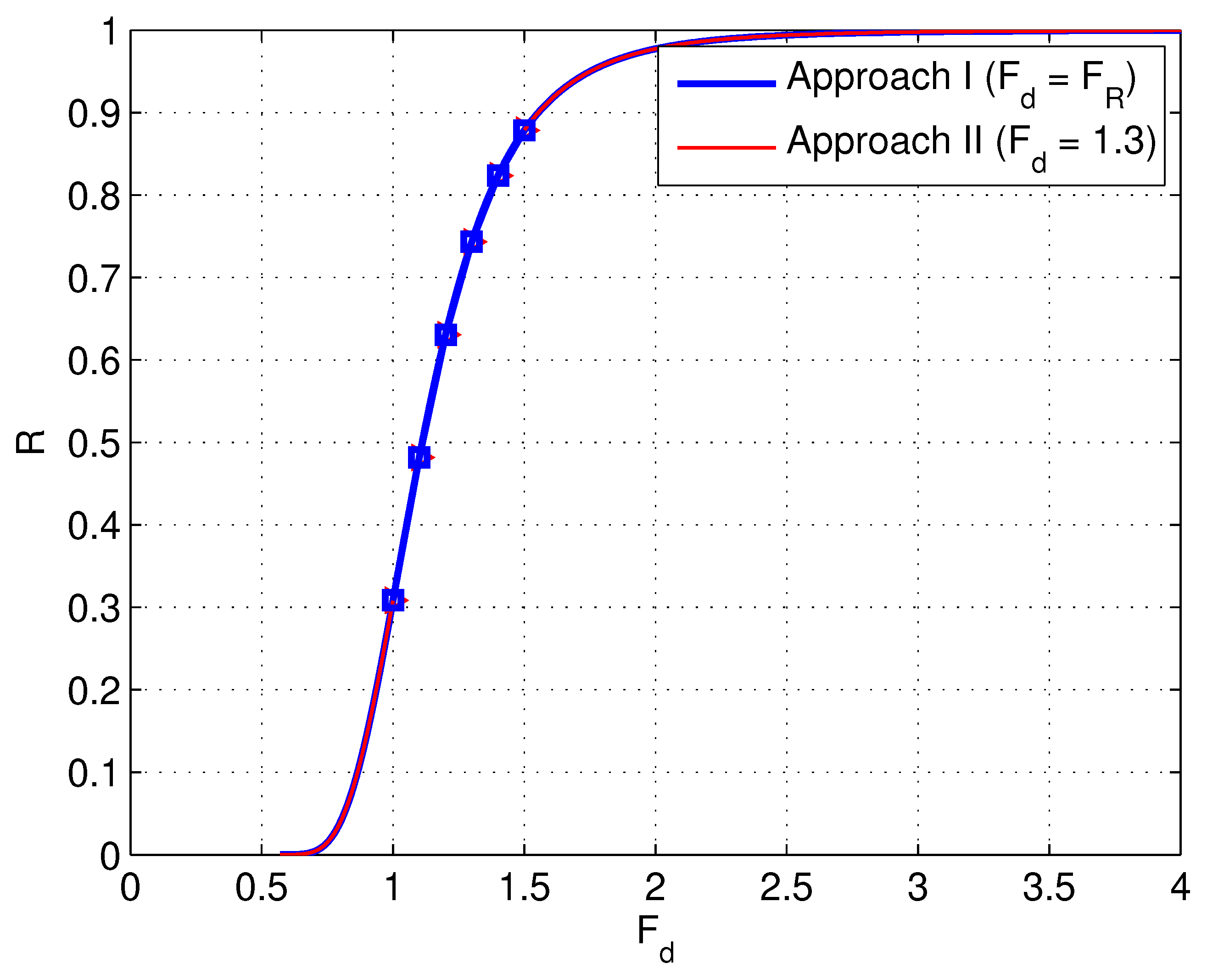
The results from the base case of
(
and
) is shown in
Figure 12 for the two cases: (1) when prescribing
(the discrete points in the figure); (2) when prescribing
(i.e., the series of values of
from the base case).
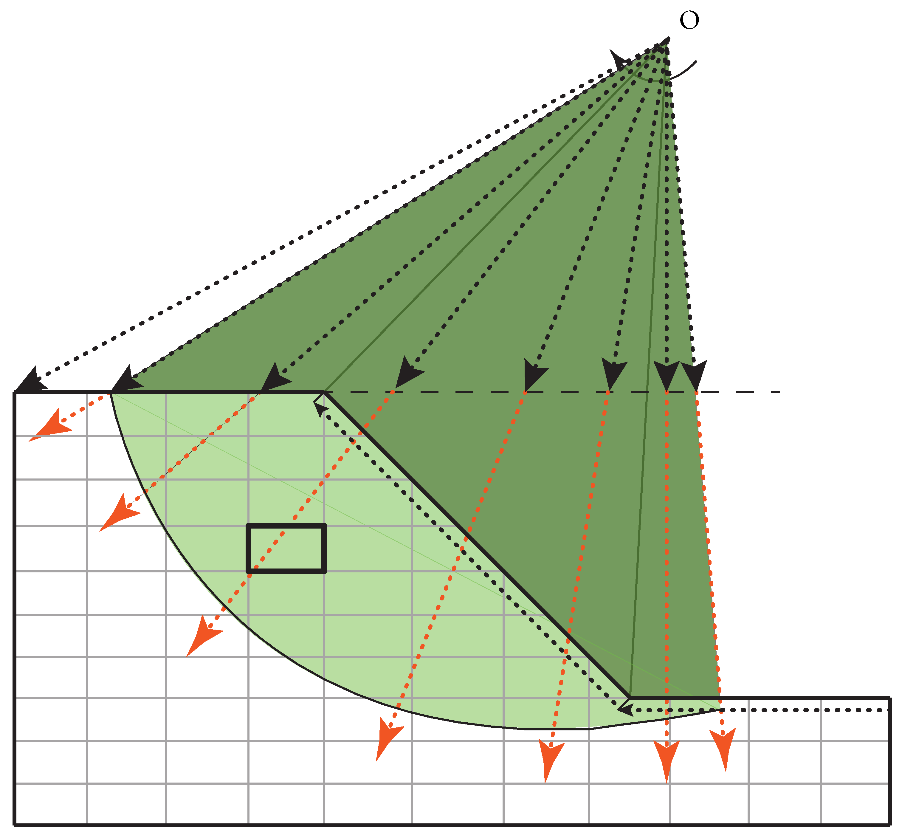
For approach I, if the slope fails for a trial factor (SRF) of 1.0, the realised
could be some value smaller than 1.0. For instance, if the plastic iteration count reaches the limit for SRF = 1.0, it might have reached the limit for SRF = 0.9, or some value that is smaller than 1.0. However, it did not really get the
for those realisations that fail (
). They were assumed to be 1.0, consequently,
was assumed to be
(Equation (
6)). Actually, this is better illustrated in
Figure 8. With Approach I, the figure is plotted by pulling back these points sitting to the right of the vertical lines of
and
. The calculated reliability is identical for the two approaches. That is, for each given
, the probability of failure is the ratio of the number of points (realisations) sitting to the right of this,
, to the total number of points (realisations) in
Figure 8. Note that the points in any vertical line comprise all the projective points (from the base case in Approach II) sitting to the right of that line. So, if the increment of
is fine enough, e.g.,
or
, instead of the previously used
, the figure plotted using Approach I (that is, in terms of vertical lines, excluding the realisations or points that have already failed for larger
under consideration, and only including these new failed realisations or points) would be the same as that produced by Approach II.
The linear trend for failure volumes shown in
Figure 8 indicates that the volumes are smaller for higher
[
21]. As
increases or the probability of failure decreases (
Figure 7), the potential slide volumes becomes smaller. In other words, the risk associated with a higher global factor of safety (
) may be relatively low, due to the low probability of failure and a decreased likelihood of large slide volumes (or an increased trend of small slide volumes). However, it will be shown that Approach I may result in underestimated sliding volumes at low failure probability levels and thereby underestimated risk (i.e., unconservative).
Note that with Approach I, the slopes that have failed for larger
will definitely fail for small
(the possibility of improving the code efficiency arises for code blocks 1 and 2, i.e., by letting the series of values of
starts with a larger value and gradually decreases by some step size, this way those realisations that have failed for a larger
would not be needed to be analysed for any smaller
). Because of this, the failure mechanisms for the same realisations will be more thoroughly formed for small
compared to those for larger
, and tend to be deeper. Thus, larger volumes are usually detected, as illustrated in
Figure 8 by the up-shifted points that should be projected horizontally to the line to their left side (the arrows in dotted lines show the positions that the relevant points should be projected to, and the solid arrows show the actual positions to which these points are projected). However, the effect of these up-shifted volumes on the distribution and range of possible failure volumes are unknown and difficult to clarify. This effect tends to increase the number of shifted volumes as
decreases. The worst consequence would be that part of the linear trend could possibly be attributed to the up-shifting when adopting Approach I (see the deviated trend in
Figure 8). After scrutiny, it was found that most of the realisations have the same rupture surfaces as those detected for larger
. As shown in
Figure 8, for
, which is the worst case, only eight realisations have had significantly different slide volumes compared to those for
(those realisations are 7, 20, 57, 60, 71, 76, 84, 97). This was thought to be due to the nested failure mechanisms for those realisations. Anyway, this is an integral part of the implementation of Approach I (i.e., for those slopes failed for the largest
considered, SRF = 1.0 is the trial factor; these slopes will definitely fail for smaller
under consideration, the trial factor is still 1.0, whereas a trial factor of, say, 0.9 would give the same failure extent). No effort was taken to improve this, as more time would be demanded to locate the actual limiting SRF (some value less than 1.0) for those known failures.
Due to the up-shifting effect and the necessity to refine to get a smooth reliability curve, the implementation of Approach I is thought to be a bad choice, although the calculation time might be an advantage (i.e., there is no need to search for the whole distribution of realised for each considered. However, if refined, this advantage could be counterbalanced). The implementation of Approach II is preferable, in that the volumes are distributed over the whole region for each , a whole distribution of realised can be gained and the reliability curve is smoother.
It is noted that the above is presented based on a normal distribution assumption of shear strength and thus
(Equation (
8)). For a lognormal distribution of shear strength, and thus a lognormal distribution of
, the cumulative distribution function of
is
where
is the error function.
In the case of a lognormal distribution of strength, the target log-normal random field can be represented by
where
is a normal random field given by
where
is a standard normal random field with zero mean and unit variance and
and
are given by
Assume that for a particular and a series of is obtained based on this , this is referred to as the base case. For a target , i.e., any given target value, the values need to be scaled by a factor of . For a constant coefficient of variation , and , it follows that . In turn, . Therefore, the series of for the base case can also be scaled by the same factor to give the values for the target .
Similar to the normal case, the probability of failure can be assessed by setting
in Equation (
9), i.e.,
By changing and for various values of , the reliability (i.e., ) can be assessed.
On the other hand,
where the derivation makes use of the generic form of Equation (12), i.e., for
.
That is, the reliability (i.e.,
) can be assessed by letting
in Equation (
9) and keeping
and
as the values based on the base case. Therefore, the conclusions in this paper can be considered general for the two most commonly used distribution types, i.e., normal and lognormal distribution.


