Random Field-Based Time-Dependent Reliability Analyses of a PSC Box-Girder Bridge


Abstract
:1. Introduction
2. Basic Theory of Random Field
2.1. Discretization of Random Field.
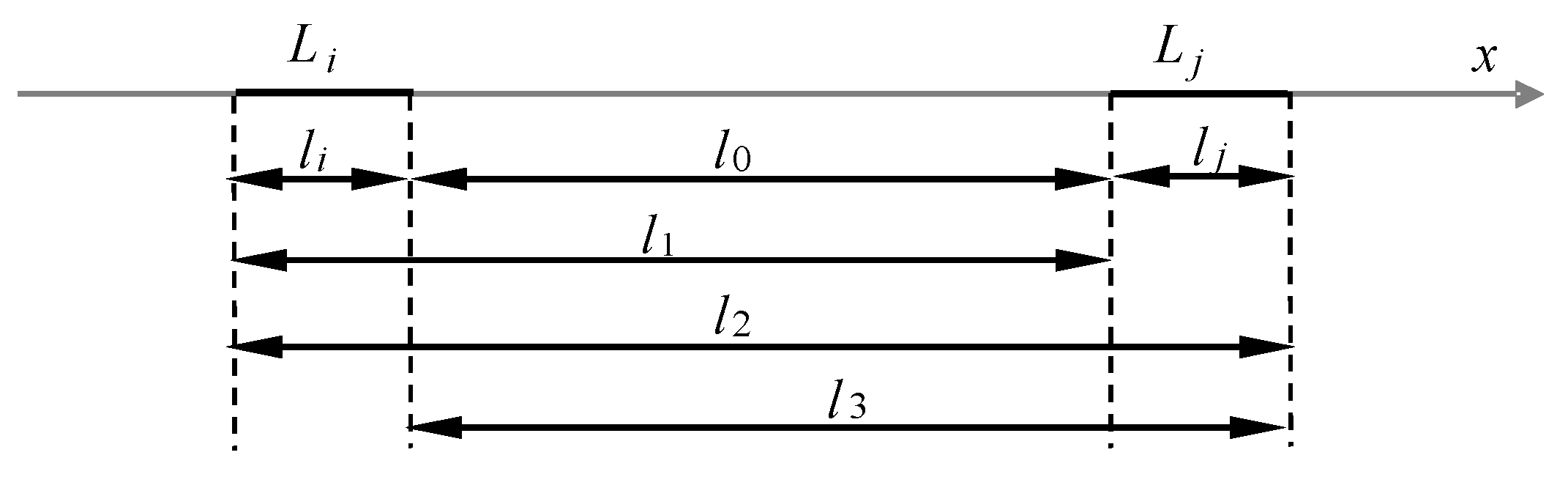
2.1.1. 1D Random Field
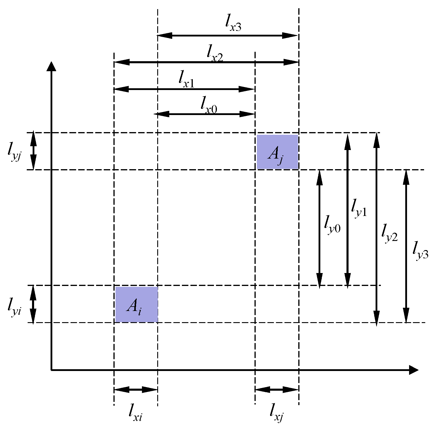
2.1.2. 2D Random Field
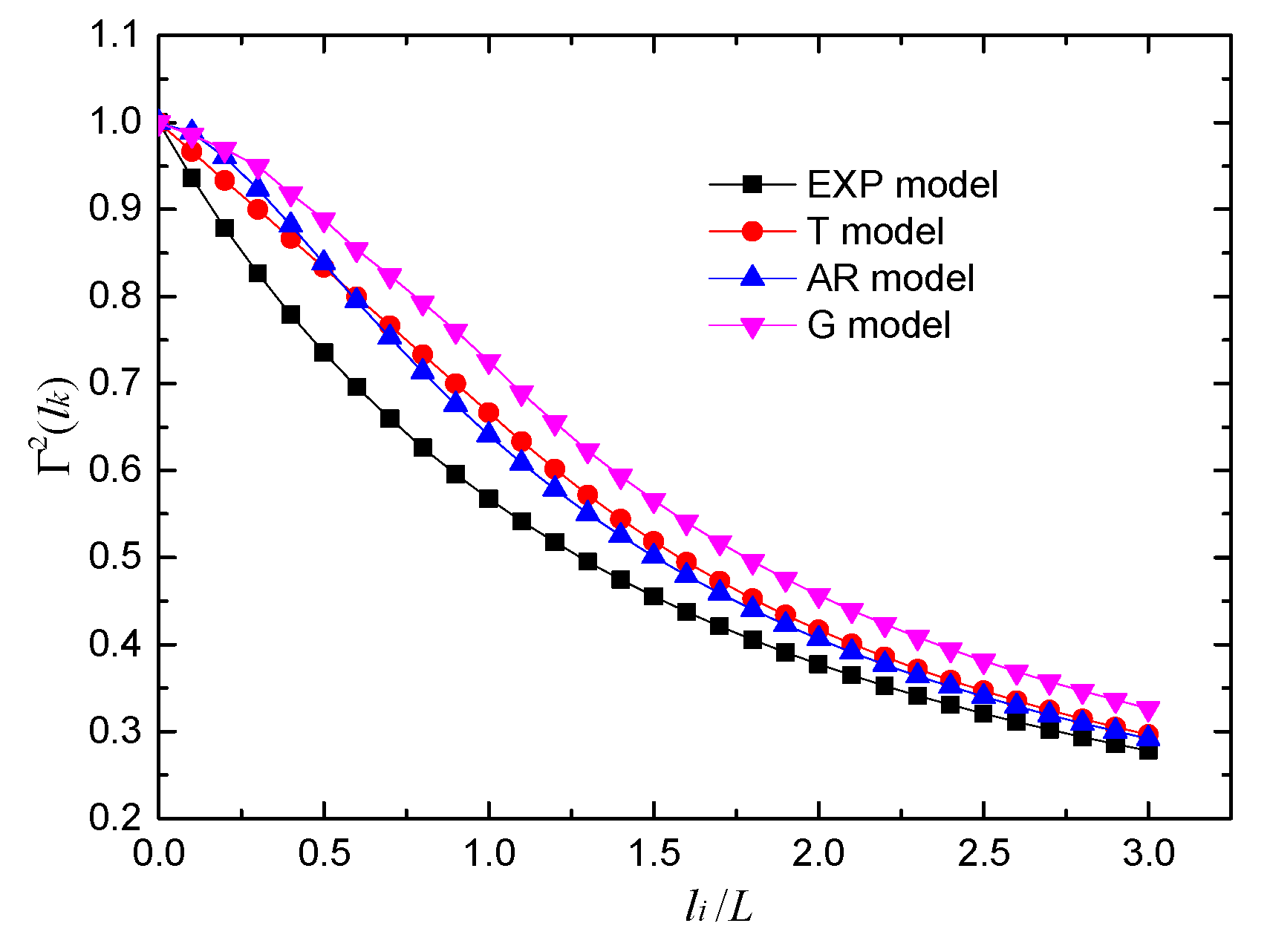
2.2. Orthogonal Transform.
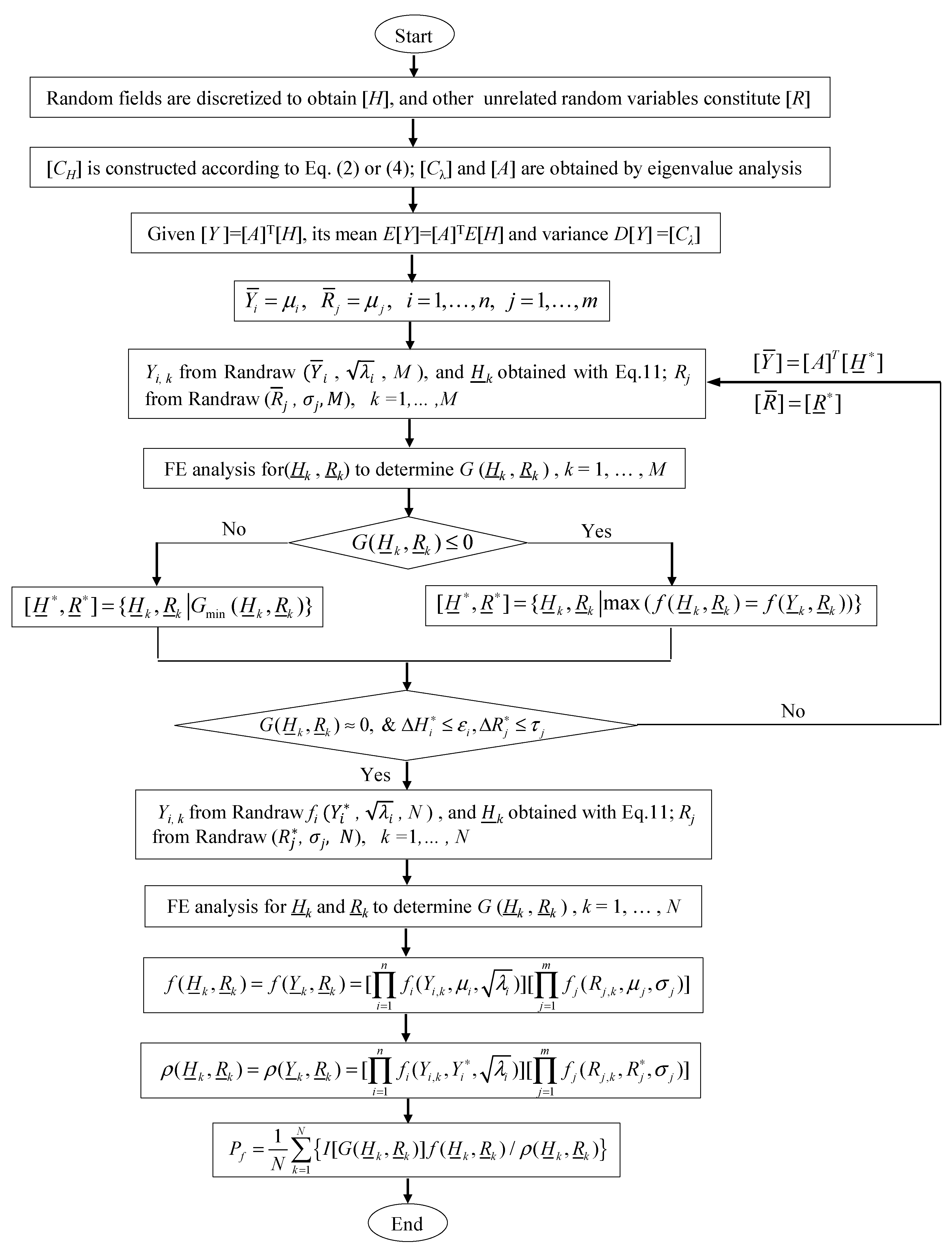
3. Structural Reliability Considering Random Field
4. Verification of Numerical Examples
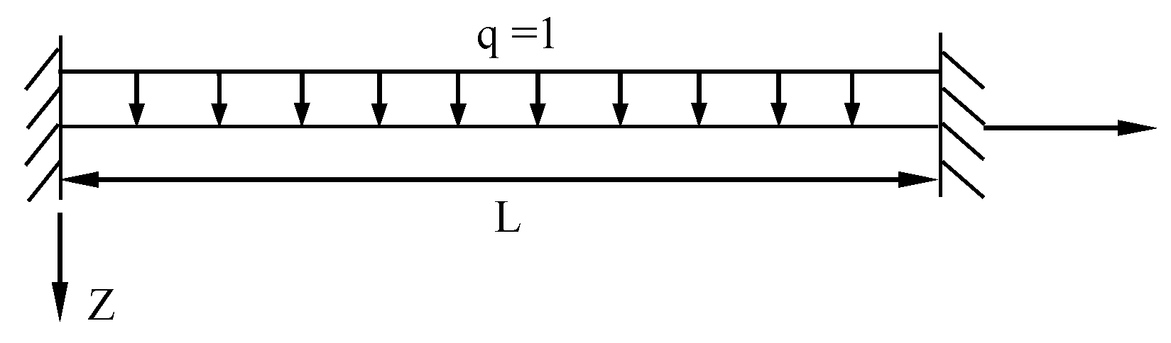
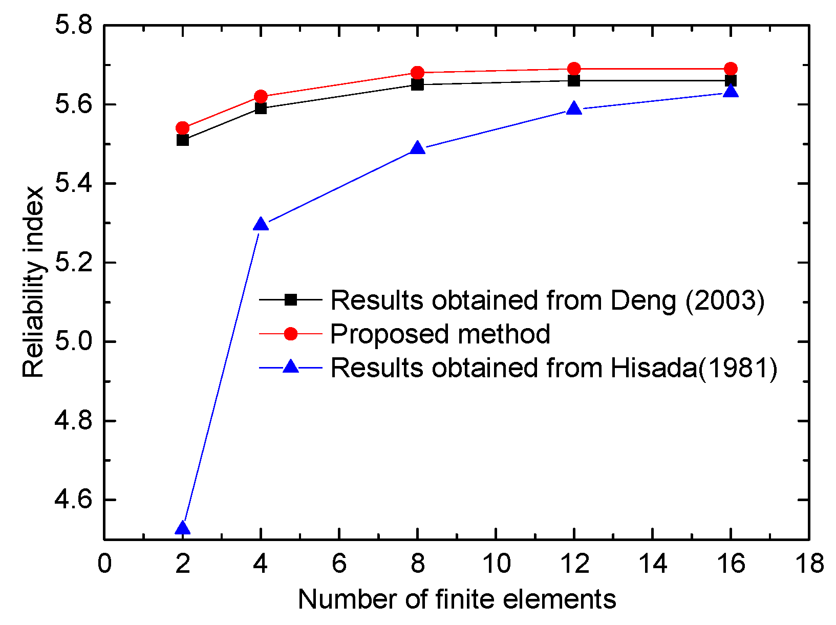
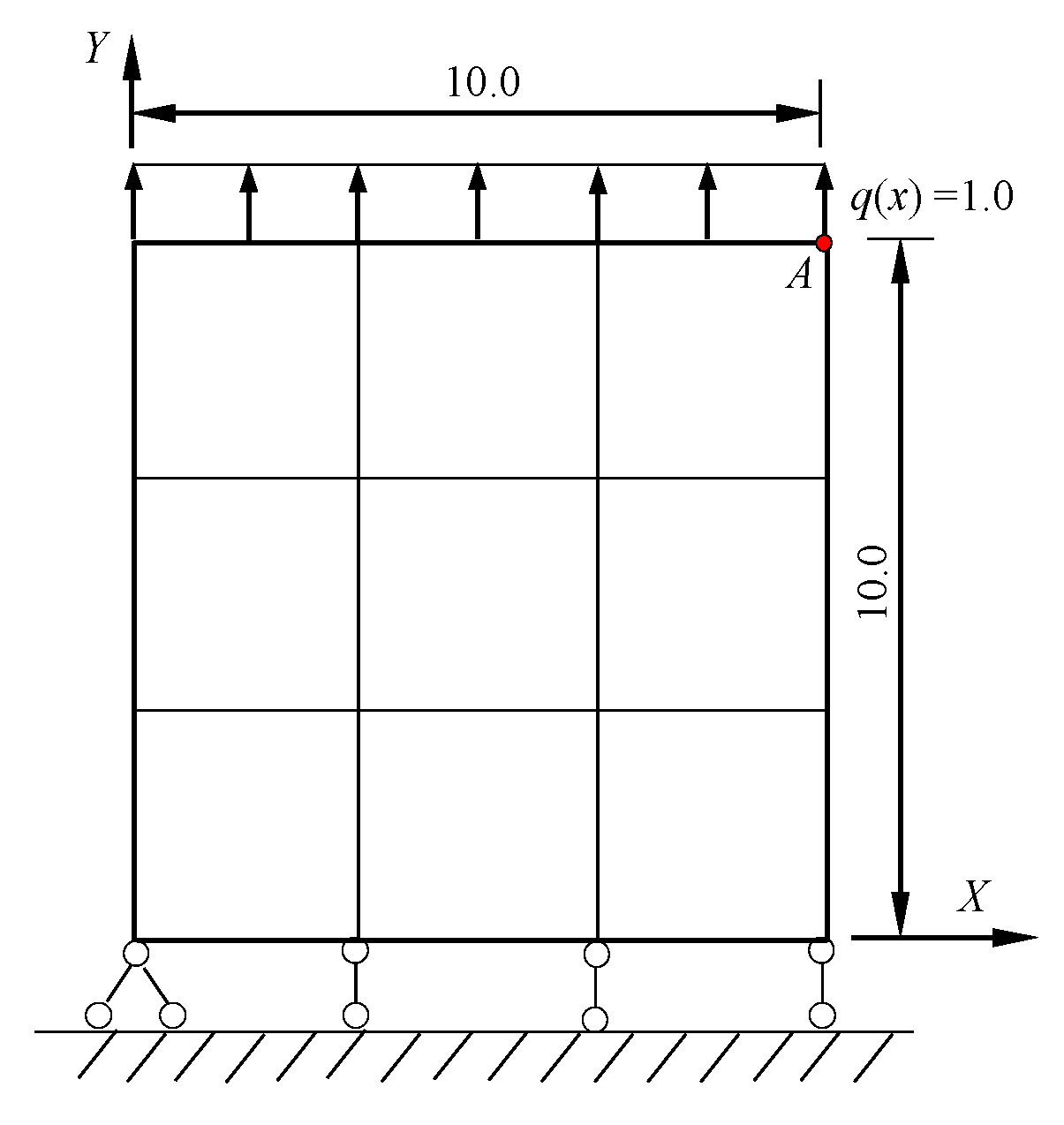
4.1. Example One
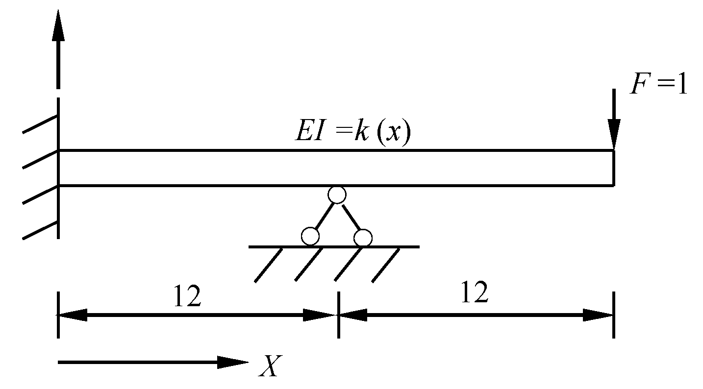
4.2. Example Two
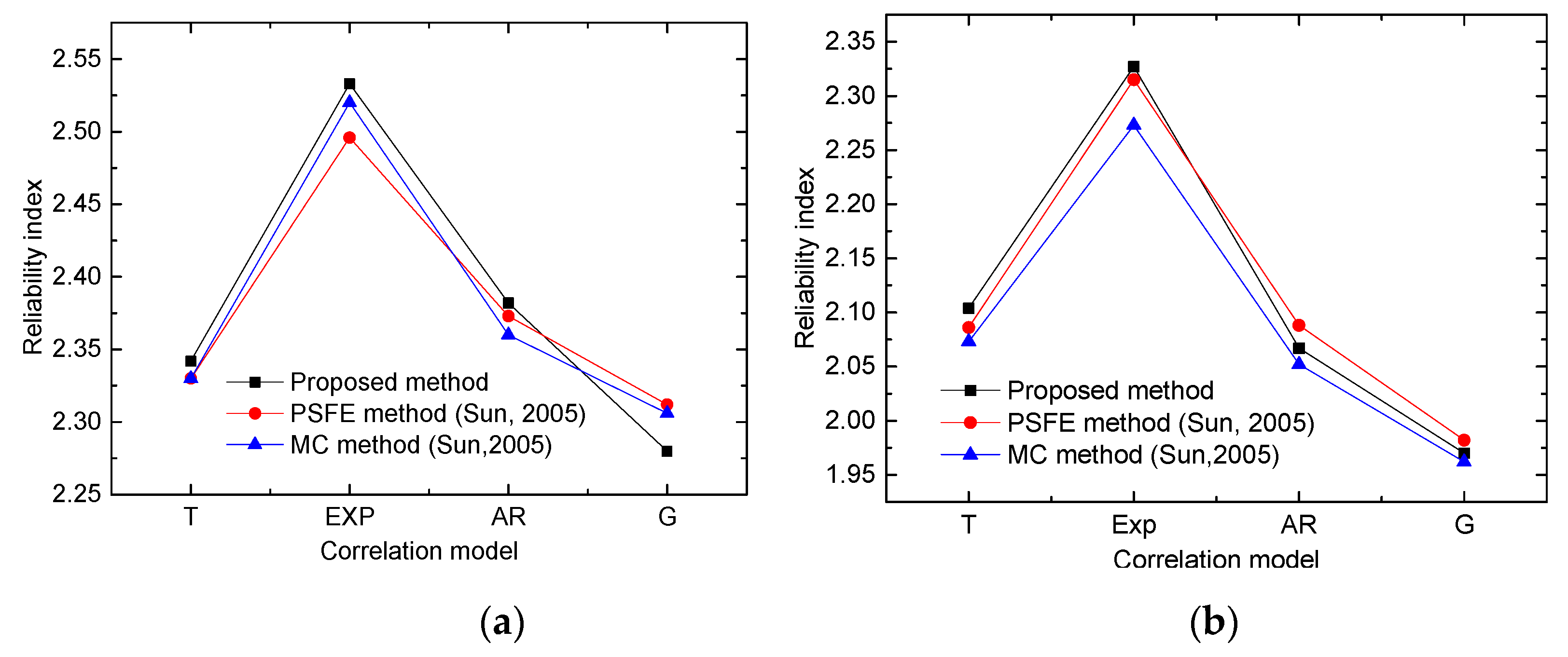
4.3. Example Three
5. Time-Dependent Reliability Analysis of the PSC Box-Girder Bridge
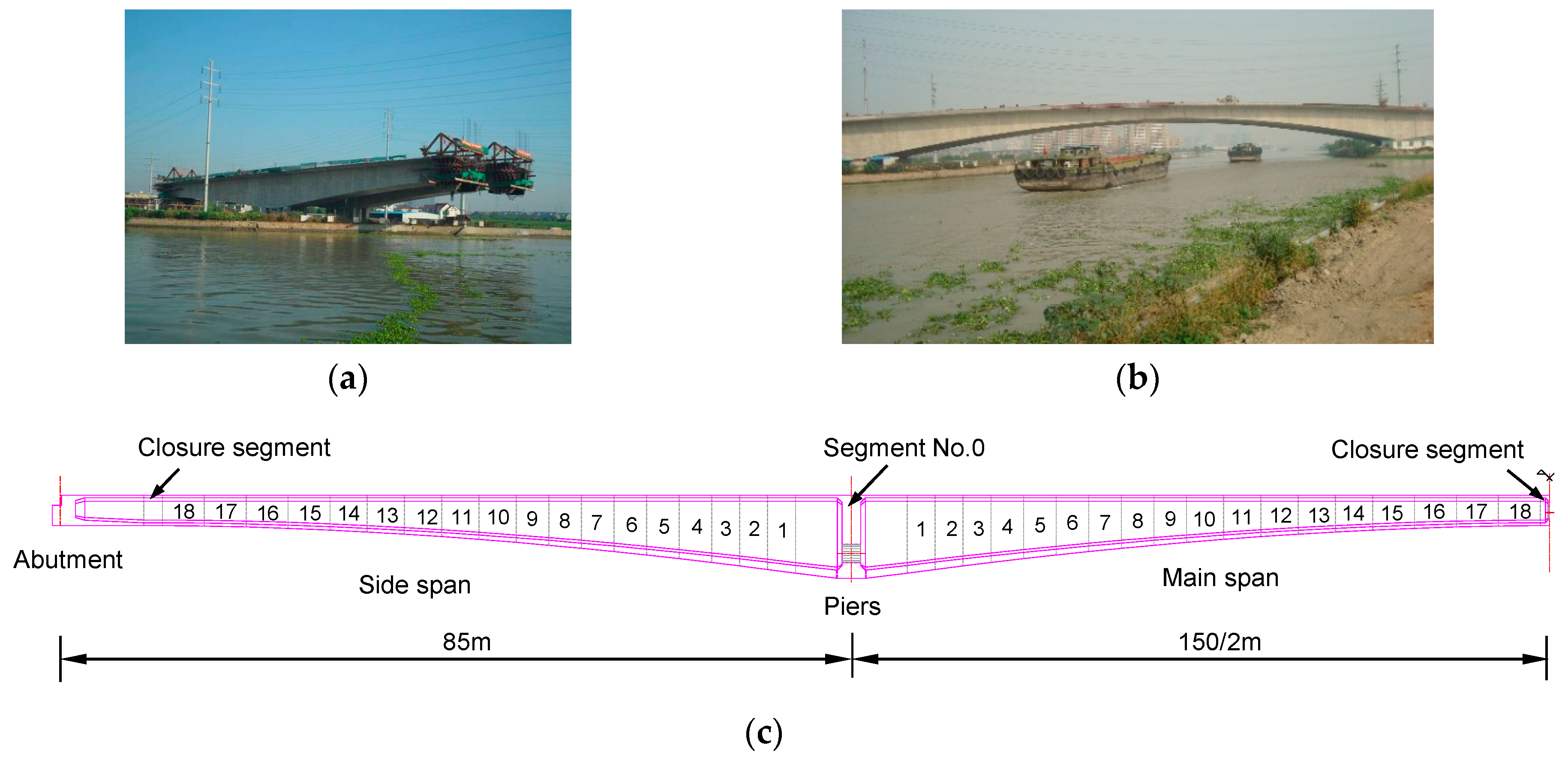
5.1. Bridge Description.
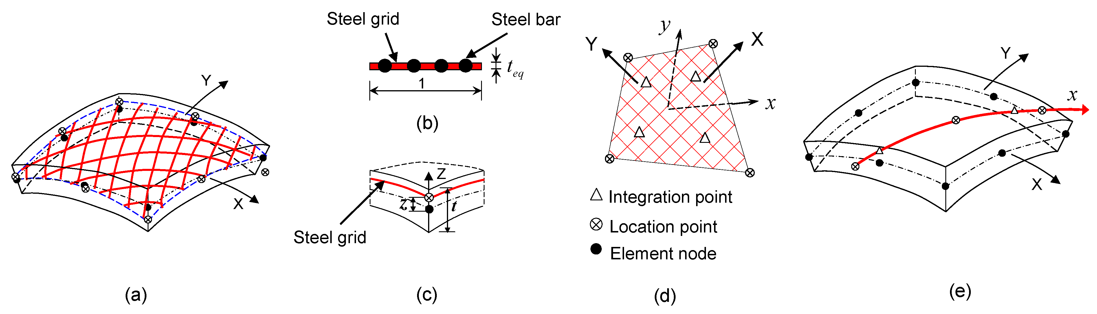
5.2. Finite Element Model
5.3. Statistical Characteristics of Random Parameters
5.4. Definition of Limit State
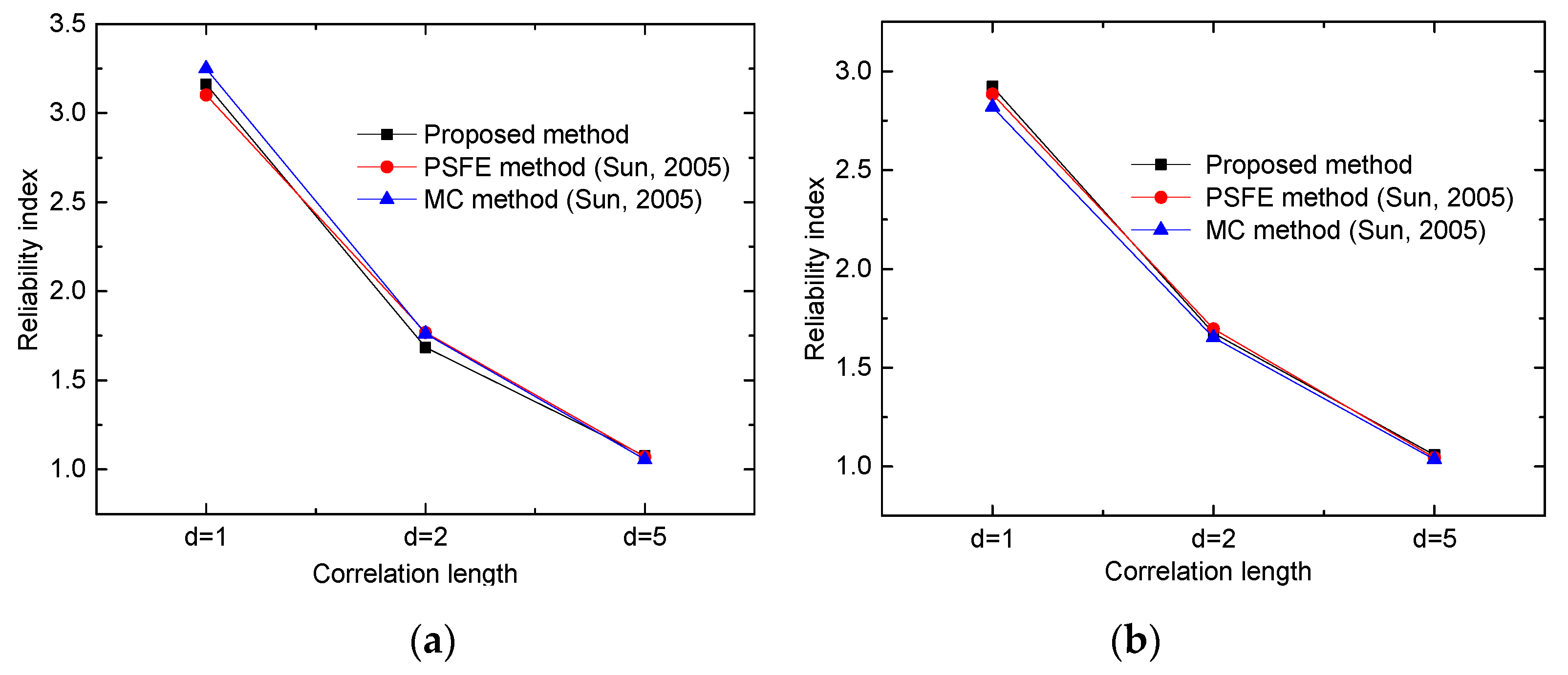
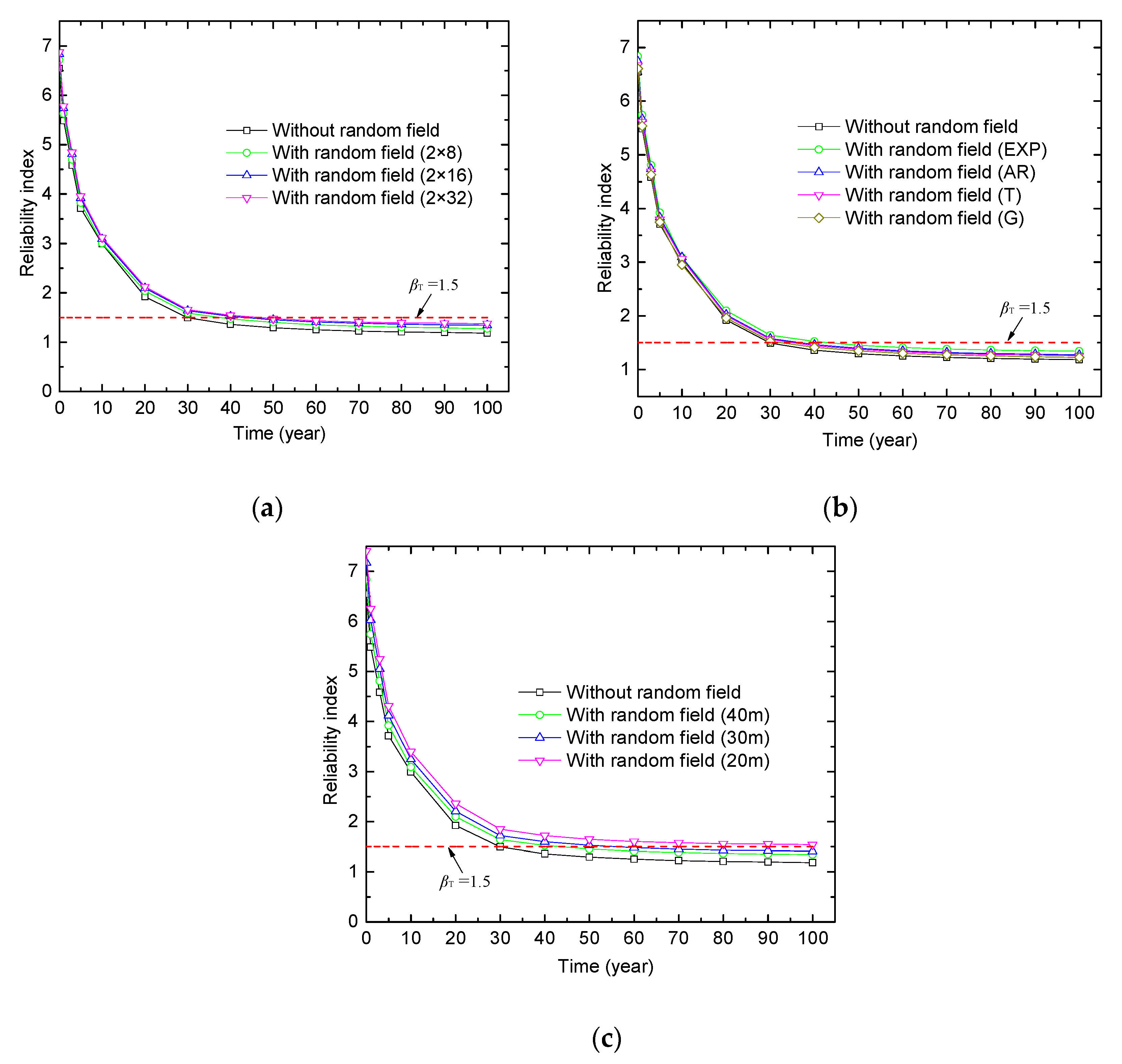
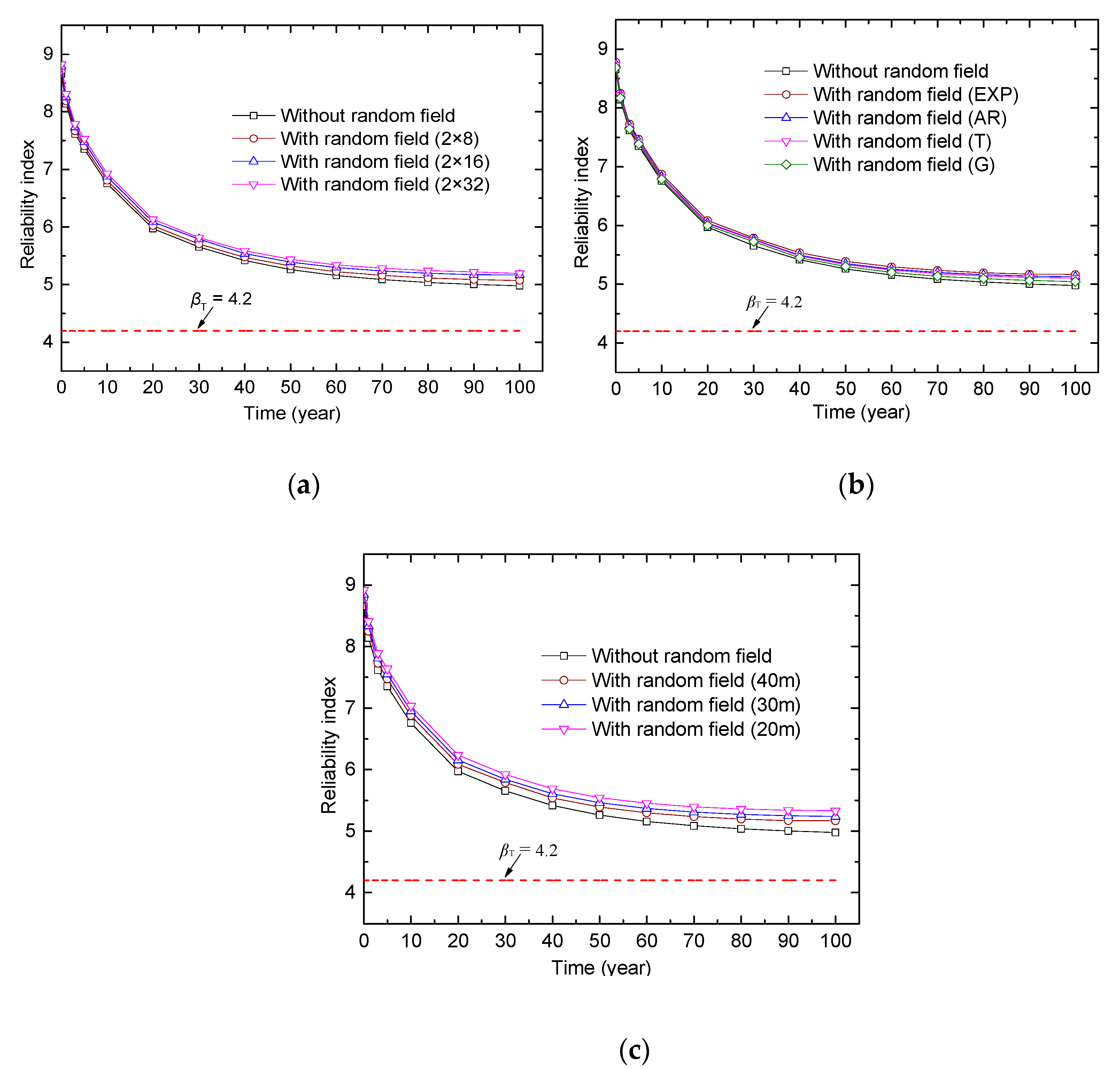
5.5. Results and Discussion.
6. Conclusions
Author Contributions
Funding
Conflicts of Interest
References
- Bazant, Z.P.; Yu, Q.; Li, G. Excessive Long-Time Deflections of Prestressed Box Girders. I: Record-Span Bridge in Palau and Other Paradigms. J. Struct. Eng. 2012, 138, 676–686. [Google Scholar] [CrossRef]
- Bazant, Z.P.; Hubler, M.H.; Yu, Q. Pervasiveness of excessive segmental bridge deflections: Wake-up call for creep. ACI Struct. J. 2011, 108, 766–774. [Google Scholar]
- Enright, M.P.; Frangopol, D.M. Probabilistic analysis of resistance degradation of reinforced concrete bridge beams under corrosion. Eng. Struct. 1998, 20, 960–971. [Google Scholar] [CrossRef]
- Coronelli, D.; Castel, A.; Vu, N.A.; François, R. Corroded post-tensioned beams with bonded tendons and wire failure. Eng. Struct. 2009, 31, 1687–1697. [Google Scholar] [CrossRef]
- Xie, H.B.; Wang, Y.F.; Wu, H.L.; Li, Z. Condition Assessment of Existing RC Highway Bridges in China Based on SIE2011. J. Bridge Eng. 2014, 19, 04014053. [Google Scholar] [CrossRef]
- Al-Harthy, A.S.; Frangopol, D.M. Reliability assessment of prestressed concrete beams. J. Struct. Eng. 1994, 1, 188–199. [Google Scholar] [CrossRef]
- Du, B.; Zhao, R.D.; Xiang, T.Y. Lifetime Reliability Analysis of Flexural Cracking for Existing Prestressed Concrete Bridge under Corrosion Attack. In Proceedings of the Tenth International Conference of Chinese Transportation Professionals (ICCTP), Beijing, China, 4–8 August 2010. [Google Scholar]
- Akgul, F.; Frangopol, D.M. Lifetime performance analysis of existing prestressed concrete bridge superstructures. J. Struct. Eng. 2004, 130, 1889–1903. [Google Scholar] [CrossRef]
- Steinberg, E. Structural reliability of prestressed UHPC Flexure models for bridge girders. J. Bridge Eng. 2010, 15, 65–72. [Google Scholar] [CrossRef]
- Nowak, A.S.; Park, C.H.; Casas, J.R. Reliability analysis of prestressed concrete bridge girders: Comparison of Eurocode, Spanish Norma IAP and AASHTO LRFD. Struct. Safety. 2001, 23, 331–344. [Google Scholar] [CrossRef]
- Du, J.S.; Au, F.T.K. Deterministic and reliability analysis of prestressed concrete bridge girders: Comparison of the Chinese, Hong Kong and AASHTO LRFD codes. Struct. Safety. 2005, 27, 230–245. [Google Scholar] [CrossRef]
- Guo, T.; Sause, R.; Frangopol, D.; Li, A. Time-dependent reliability of PSC box-girder bridge considering creep, shrinkage and corrosion. J. Bridge Eng. 2010, 16, 29–43. [Google Scholar] [CrossRef]
- Guo, T.; Liu, T.; Li, A.Q. Deflection reliability analysis of PSC box-girder bridge under high-speed railway loads. Adv. Struct. Eng. 2012, 15, 2001–2012. [Google Scholar] [CrossRef]
- Vanmarcke, E.H.; Grigoriu, M. Stochastic finite element analysis of simple beams. J. Eng. Mech. 1983, 109, 1203–1214. [Google Scholar] [CrossRef]
- Most, T.; Bucher, C. Probabilistic analysis of concrete cracking using neural networks and random fields. Probabilist Eng. Mech. 2007, 22, 219–229. [Google Scholar] [CrossRef]
- Rahman, S.; Rao, B.N. An element-free Galerkin method for probabilistic mechanics and reliability. Int. J. Solids Struct. 2001, 38, 9313–9330. [Google Scholar] [CrossRef]
- Stewart, M.G. Spatial variability of pitting corrosion and its influence on structural fragility and reliability of RC beams in flexure. Struct. Safety. 2004, 26, 453–470. [Google Scholar] [CrossRef]
- Stewart, M.G.; Mullard, J.A. Spatial time-dependent reliability analysis of corrosion damage and the timing of first repair for RC structures. Eng. Struct. 2007, 29, 1457–1464. [Google Scholar] [CrossRef]
- Cheng, J. Random field-based reliability analysis of prestressed concrete bridges. KSCE J. Civ. Eng. 2014, 18, 1436–1445. [Google Scholar] [CrossRef]
- Yang, I.H. Uncertainty and sensitivity analysis of time-dependent effects in concrete structures. Eng. Struct. 2007, 29, 1366–1374. [Google Scholar] [CrossRef]
- Vanmarcke, E.H. Probabilistic modeling of soil profiles. J. Geotech. Eng. Div. 1977, 103, 1227–1246. [Google Scholar]
- Kiureghian, D.A.; Ke, J.B. The stochastic finite element method in structural reliability. Probab. Eng. Mech. 1988, 3, 83–91. [Google Scholar] [CrossRef]
- Liu, W.K.; Belytschko, T.; Mani, A. Random field finite elements. Int. J. Numer. Meth. Eng. 1986, 23, 1831–1845. [Google Scholar] [CrossRef]
- Beacher, G.B.; Ingra, T.S. Stochastic FEM in settlement predictions. J. Geotech. Geoenviron. 1981, 107, 449–463. [Google Scholar]
- Zhu, W.Q.; Wu, W.Q. On the local average of random field in stochastic finite element analysis. Acta Mech. Solida Sin. 1990, 3, 27–42. [Google Scholar]
- Takada, T.; Shinozuka, M. Local integration method in stochastic finite element analysis. In Proceedings of the 5th International Conference on Structural Safety and Reliability, San Francisco, CA, USA, 7–11 August 1989. [Google Scholar]
- Spanos, P.D.; Ghanem, R. Stochastic finite element expansion for Random media. J. Eng. Mech. 1989, 115, 1035–1053. [Google Scholar] [CrossRef]
- Li, C.C.; Kiureghian, D.A. Optimal discretization of random Fields. J. Eng. Mech. 1993, 119, 1136–1154. [Google Scholar] [CrossRef]
- Vanmarcke, E.; Shinozuka, M.; Nakagiri, S.; Schueller, G.I.; Grigoriu, M. Random fields and stochastic finite element method. Struct. Safety. 1986, 3, 143–166. [Google Scholar] [CrossRef]
- Liu, P.L.; Liu, K.G. Selection of random field mesh in finite element reliability analysis. J. Eng. Mech. 1993, 119, 667–680. [Google Scholar] [CrossRef]
- Au, S.K.; Beck, J.L. A new adaptive importance sampling scheme for reliability calculations. Struct. Safety. 1999, 21, 135–158. [Google Scholar] [CrossRef]
- Deng, S.M. Structural Reliability Analysis of Thin-Walled Box Girders Based on Stochastic Finite Element Method. Master’s Thesis, Guangxi University, Nanning, China, 2003. (In Chinese). [Google Scholar]
- Hisada, T.; Nakagiri, S. Stochastic finite element method developed for structural safety and reliability. In Proceedings of the 3rd International Conference on Structural Safety and Reliability, Trondheim, Norway, 23–25 June 1981. [Google Scholar]
- Sun, C. Numerical Techniques for Structural Reliability Analysis of Thin-Walled Box Girders in Generalized Random Space. Master’s Thesis, Guangxi University, Nanning, China, 2005. (In Chinese). [Google Scholar]
- Manie, J.; Kikstra, W.P. DIANA. User’s Manual-Element Library; Release 9.3; TNO Building and Construction Research, TNO DIANA BV: Delft, The Netherlands, 2008. [Google Scholar]
- CEB-FIP. CEB-FIP Model Code 1990: Design Code 1994. Thomas Telford, London, 1994. Available online: https://scholar.xiayige.org/scholar?hl=zh-CN&as_sdt=0%2C5&q=CEB-FIP+model+code+1990%3A+Design+code+1994&btnG= (accessed on 10 August 2018).
- RILEM TC-107-GCS. Creep and shrinkage prediction models for analysis and design of concrete structures—Model B3. Mater. Struct. 1995, 28, 357–365. [Google Scholar] [CrossRef]
- CEN (Standardization European Committee). Design of Concrete Structures. Part 1-1: General Rules and Rules for Buildings; Eurocode 2 EN 1991-1-1; CEN: Brussels, Belgium, 2004. [Google Scholar]
- ACI (American Concrete Institute). Prediction of Creep, Shrinkage and Temperature Effects in Concrete Structures; ACI-209R-82; ACI: Detroit, MI, USA, 1982. [Google Scholar]
- Gardner, N.J.; Lockman, M.J. Design provisions for drying shrinkage and creep and normal-strength concrete. ACI Mater. J. 2001, 98, 159–167. [Google Scholar]
- Goel, R.; Kumar, R.; Paul, D.K. Comparative study of various creep and shrinkage prediction models for concrete. J. Mater. Civ. Eng. 2007, 19, 249–260. [Google Scholar] [CrossRef]
- Madsen, H.O.; Bazant, Z.P. Uncertainty analysis of creep and shrinkage effects in concrete structures. ACI J. 1983, 82, 116–127. [Google Scholar]
- GBT50283-1999. Unified Standard for Reliability Design of Highway Engineering Structures; China Planning Press: Beijing, China, 1999. (In Chinese) [Google Scholar]
- Zhang, Y.T.; Meng, S.P. Prediction of long-term deformation of long-span continuous rigid frame bridges using the response surface method. J. China Civ. Eng. 2011, 44, 102–106. (In Chinese) [Google Scholar]
- Guo, T.; Chen, Z.H. Deflection control of long-span PSC box-girder bridge based on field monitoring and probabilistic FEA. J. Perform. Constr. Fac. 2016, 30, 04016053. [Google Scholar] [CrossRef]
- Ministry of Transport of the People’s Republic of China. Code for Design of Highway Reinforced Concrete and Prestressed Concrete Bridges and Culverts; (JTG D62-2004); China Communication Press: Beijing, China, 2004. (In Chinese)


| Random Field | Mean | Coefficient of Variation (COV) | Distribution | Correlation Model | Correlation Length |
|---|---|---|---|---|---|
| E (MPa) | 10 | 0.01 | Normal | Exp | 10 m |
| I (m4) | 0.6667 | 0.01 | Normal | Exp | 10 m |
| Random Variables | Unit | Mean | COV | Distribution | Data Sources |
|---|---|---|---|---|---|
| Creep uncertain coefficient ψ1 | — | 1 | 0.339 | Normal (truncated at 0) | Reference [42] |
| Shrinkage uncertain coefficient ψ2 | — | 1 | 0.450 | Normal (truncated at 0) | Reference [42] |
| Density of concrete DC | kN/m3 | 25.5 | 0.046 | Normal (truncated at 0) | Reference [43] |
| Control prestressing stress σcon | MPa | 1395 | 0.040 | Normal (truncated at 1488) | Reference [44] |
| Concrete strength fcm28 | MPa | 63.9 | 0.089 | Normal (truncated at 40) | Concrete strength test |
| Relative humidity RH | % | 67.3 | 0.191 | Normal (truncated at 100) | China Meteorological Administration |
| Loading age t0 | d | 7 | 0.110 | Uniform | Design assumption |
| Random Field | Mean | COV | Distribution | Correlation Model | Correlation Length |
|---|---|---|---|---|---|
| Elastic modulus (GPa) | 36.8 | 0.09 | Normal | Exp | 40 m |
| Secondary dead load (kN/m) | 60.3 | 0.11 | Normal | Exp | 40 m |
| Live load (kN/m) | 21.0 | 0.19 | Normal | Exp | 40 m |
© 2019 by the authors. Licensee MDPI, Basel, Switzerland. This article is an open access article distributed under the terms and conditions of the Creative Commons Attribution (CC BY) license (http://creativecommons.org/licenses/by/4.0/).
Share and Cite
Chen, Z.; Guo, T.; Liu, S.; Lin, W. Random Field-Based Time-Dependent Reliability Analyses of a PSC Box-Girder Bridge. Appl. Sci. 2019, 9, 4415. https://doi.org/10.3390/app9204415
Chen Z, Guo T, Liu S, Lin W. Random Field-Based Time-Dependent Reliability Analyses of a PSC Box-Girder Bridge. Applied Sciences. 2019; 9(20):4415. https://doi.org/10.3390/app9204415
Chicago/Turabian StyleChen, Zheheng, Tong Guo, Shaobo Liu, and Weiwei Lin. 2019. "Random Field-Based Time-Dependent Reliability Analyses of a PSC Box-Girder Bridge" Applied Sciences 9, no. 20: 4415. https://doi.org/10.3390/app9204415
APA StyleChen, Z., Guo, T., Liu, S., & Lin, W. (2019). Random Field-Based Time-Dependent Reliability Analyses of a PSC Box-Girder Bridge. Applied Sciences, 9(20), 4415. https://doi.org/10.3390/app9204415