Assembly Tolerance Design Based on Skin Model Shapes Considering Processing Feature Degradation

Abstract

To increase the reliability and accuracy of tolerance design, more and more research works are considering not only orientation and position deviations; they are also forming errors in tolerance modeling. As a direct cause of form errors in industrial mass production, the processing features of the machining system degrade over time. Under the Industry 4.0 paradigm, an assembly tolerance design method based on Skin Model Shape is proposed to take the effect of degrading processing features into consideration. A continuous-time multi-dimensional Markov process is trained through maximum likelihood estimation based on the nodal sampling point set on the machined surface. Degradation of the machined surface is modeled based on the joint probability distribution of nodal displacements. Assembly force constraints and assembly entity constraints are applied to spatial assembly simulations. Tolerance synthesis takes the manufacturing cost and assembling probability as design objectives. A design example of the rotary feed component in a five-axis machine tool is proposed for explanation and verification.

1. Introduction

Under the innovative concept of Industry 4.0, automated and digitized systems in smart factories could enable the real-time integration and analysis of massive amounts of data by the use of electronics and information technologies. Moreover, this would finally result in a more flexible and optimized manufacturing process [1,2,3]. This theory points to the improvement of intelligent solutions in the tolerance design of mechanical products, including the replacement of empiricism with knowledge-intensive and data-based processes. The general practice of mechanical tolerance design is to treat tolerance design as a combination of tolerance modeling, assembly simulating, tolerance allocation, and optimization. The best combination of part tolerance is assigned through multi-dimensional objective constraints in order to meet environmental clearance, conform to functional requirements, improve product quality, and lower manufacturing costs in the late design stage [4,5,6]. To increase the accuracy and robustness of the designed tolerance scheme, the influence of processing feature degradation caused by machining precision deterioration is taken into consideration.

In the past few decades, researchers have presented several efficient computer-aided methods for estimating geometry variation and product tolerance. Many models have been developed for geometrical feature representation, deviation accumulation, and tolerance zone estimation [7]. Conventional tolerance modeling methods are mainly categorized into those based on vector loops, Tolerance-Map (T-Map), small displacement torsor (SDT), a Homogeneous Transformation Matrix (HTM), and some other innovative models. Vector loops provide vectorial tolerance representation and analysis for the surfaces of different components. However, only five standard surfaces are typically considered (plane, cylinder, sphere, cone, and torus) [8,9,10,11]. Consisting of a hypothetical volume of points, a T-Map contains all the possible locations for geometrical features, and is used to illustrate the accumulation of product variations [12,13,14]. The SDT model uses screws and constraints to establish the extreme limits of part tolerance zones [15,16,17]. To overcome the lack of analytical models between the target feature and each feature on the dimensional chain, HTM was combined with T-Map to obtain an expression of the decoupling pose of tolerance features [18]. Since the Jacobian matrices are quite suitable for deviation propagation [19], the unified Jacobian–Torsor model was developed for product precision performance estimation [20,21,22]. Furthermore, some innovative modeling methods, such as neural network [23], volumetric envelope [24], modal analysis [25,26] and graph theory [27,28] have also been applied to model the mating tolerance of both parts and assemblies. Some of the aforementioned models have contributed to the mainstream commercial computer-aided tolerancing software, such as 3DCS Variation Analyst, eM-TolMate, VisVSA, and CETOL 6 Sigma [29]. However, most of these tolerancing models excel at estimating the precision of a mechanical product at one state, while they cannot adapt to simulate a sequence of degradation trajectories. Moreover, the simplification of form deviation into a series of tiny dimensional, rotational, and translational deviations of geometric features in some of these models brings about inaccurate virtual representation in the modeling stage and unneglectable simulation errors in the synthesizing and optimizing stages.

As a response, the Skin Model Shape theory was introduced as a new paradigm for the modeling of product geometry considering shape variability. The theory of Skin Model Shapes is an integration of international geometric standards and the concept of the Skin Model [30,31,32,33]. Within the theoretical framework of GeoSpelling [34], the Skin Model Shape is commonly formed by discrete geometry schemes such as point clouds and surface meshes. It provides an approach for the employment of computational techniques on the Skin Model. Research studies have shown that the Skin Model Shape has great efficiency for the representation of product geometry considering geometrical deviations and form errors [29,35,36]. Besides, since deviations in the Skin Model Shape are generated mainly by duplicating a sample pattern from the non-ideal manufacturing process, real part measurement, shape defect simulation, and statistical shape analysis are employed on Skin Model Shapes for convenience. For example, finite element analysis is introduced to help reduce local modeling drawbacks and improve model quality [37]. In addition, the discrete form of the Skin Model Shape has been proven to have great potential in further assembly simulation, performance evaluation, and tolerance analysis [38,39,40].

Significant efforts have been made to improve the accuracy of product models when processing features are taken into consideration. Processing features, including systematic geometric deviations and microscopic form patterns, are essentially affected by and have been employed as an estimation for the performance of machine tools. The pattern of machining defects is detected in order to provide a comparison between the ideal model and the actual machining result, which is usually obtained by a coordinate measuring machine [41]. Most of the previous research has identified the machining state as a Boolean attribute: precision reliable or precision failure. If the measured degradation reaches a threshold, precision failure occurs, and the product fault time is defined. However—mainly due to the wear of the driving system, transmission gear, and cutting tool—a stochastic process, rather than binary classification, is more suitable for simulating and predicting the deterioration of machining precision and degradation of processing features. Sun et al. [42] emphasized that tool wear is a dynamic process extending from sharp to worn and possibly to breakage, and that multi-state classification could provide a more timely and accurate estimation. Dai et al. [43] pointed out that the degradation paths would be different between one product and another. They conducted a comparison of Gaussian and logarithmic distribution in order to establish the degradation model. Ozcelik and Bayramoglu [44] verified the effect of tool wear on machining surface roughness and established a statistical model for prediction under various cutting conditions. Shu et al. [45] made the assumption that the next state of machine tool wear only depends on its current wear state. So, a non-homogeneous continuous-time Markov process model was used for modeling the total experience over the target life. After that, a linear mixed-effects model and maximum likelihood estimation was implemented to assess the wear evolution and lifetime of the tool [46]. Distribution of the residual life up to the wear threshold and estimation of the wear level have also been researched. Moghaddass and Zuo [47] modeled the gradual degradation of a mechanical device as a continuous-time degradation process with multiple discrete states. A condition-monitored device based on an unsupervised parameter estimation method was developed with only incomplete information observable. A homogeneous continuous-time, finite-state semi-Markov model was established based on the past history of components by Cannarile et al. [48]. It was verified to be of great help in improving the diagnostic performance of an empirical classification system involving the degradation of mechanical systems. These applications of stochastic processes in manufacturing modeling have shown great potential in simulating the tolerance of a large branch of mechanical products in mass production based on measuring data.

The intention of this paper is to propose a solution to assembly tolerance design problems considering processing feature degradation. These problems are commonly encountered in the practical production of equipment manufacturing in industries such as high-precision computer numerical control machining, aeronautics, and astronautics. This paper focuses on assemblies containing observable parts (mainly outsourced parts, such as standard components or ultra high-precision parts) and predictable parts (mainly self-made parts, such as lathe beds, columns, and pillars). These two kinds of parts are treated in different ways—sampling and measuring are usually implemented on the observable parts for precise and detailed modeling, while the predictable parts are modeled through mathematical simulations of the geometric tolerance, form errors, and assembly clearance. Some of the tolerance indices are given through measurements, while the to-be-designed tolerance indices are assumed and experimented repeatedly. Feature precision degradation is taken into consideration in tolerance modeling to enhance the reliability and robustness of a designed tolerance scheme. As a solution, a continuous-time variational multi-dimensional Markov process is introduced for modeling the degradation process, and the degraded surfaces are used in assembly simulations. On that basis, target assembly tolerance indices are synthesized through a series of numerical experiments. As a goal, a reduction in manufacturing cost and a guarantee in assembling probability is expected through the integration of these methods to the existing tolerance design framework, especially for products in mass production.

To achieve this, a tolerance design method considering processing feature degradation is proposed. The Skin Model Shapes form is adapted as a geometric basis. The nodal sampling point set on the machined surface is obtained by means of a high-precision coordinate measuring machine. A continuous-time multi-dimensional Markov process is trained to calculate the nodal displacement joint probability distribution on the machined surfaces. The degraded machined surfaces are predicted and applied in subsequent numerical experiments. To provide the precise assembly tolerance indices, assembly simulations and data analysis are conducted, and the assembly force constraints and assembly entity constraints are taken into consideration. Then, these tolerance indices are synthesized to provide tolerance schemes with low manufacturing costs and high assembly probabilities. Estimation and verification of the efficiency of the proposed method are illustrated through an example of the transmission shaft on a five-axis high-precision machine tool (VTM200F).

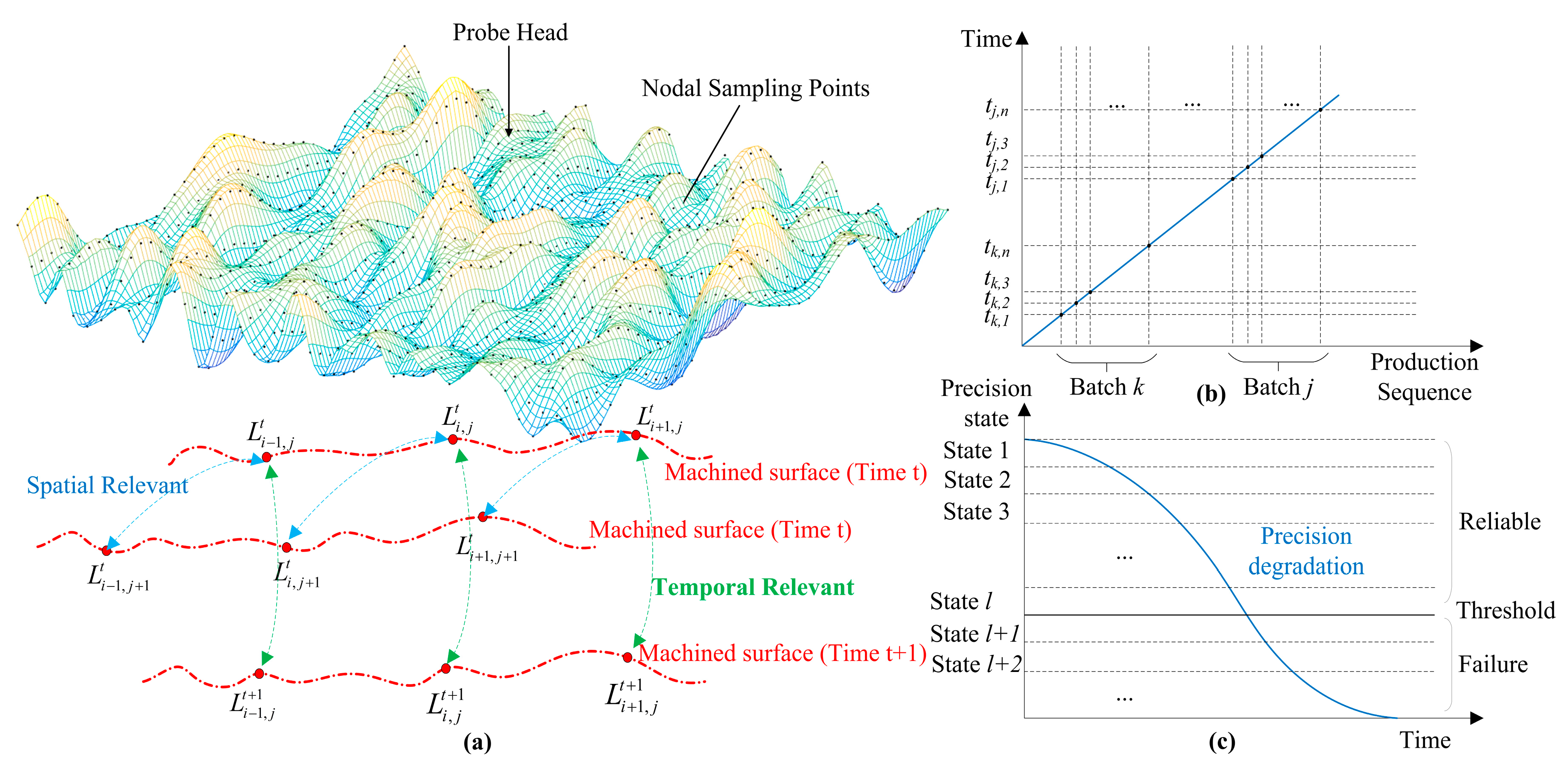
2. Predictive Machined Surface Modeling

In this paper, machined surfaces are regarded as an integration of processing features and random geometric deviation. To a specific machine surface, the processing feature is determined by the basic geometric shape (plane, cylinder, sphere, etc.), the application and sequence of processing techniques (turning, milling, grinding, etc.), and the corresponding operating parameters (cutting speed, feed rate, cutting depth, etc.). Random geometric deviation depicts unpredictable and inevitable machining errors. Previous research has shown the rationality behind the idea that a stochastic process could represent the precision deterioration of a machining system. In the condition of mass production, the processing features are degrading due to the deterioration of the machining tool. Therefore, a multi-dimensional Markov model based on data training is introduced for modeling and prediction. The pattern of degradation becomes more explicit if the machined parts are from different branches.

2.1. Modeling of the Multi-Dimensional Markov Process

The multi-dimensional Markov model is presented in this section, and a machined surface is used as an example. A uniform grid with a sampling interval $\Delta$ is placed on the nominal machined surface. The measuring process is calibrated through the grid nodes. A high-precision coordinate measuring machine is used to obtain the actual coordinates of sampling points on the real surface. The coordinate set is called the nodal sampling point set $\Omega$. To a plane, the sampling interval Δ is a set distance along the x-direction and y-direction in the local machining coordinate system. To a spherical or cylindrical surface, the sampling interval $\Delta$ is a set angle around the central point or central axis.

First, we use $P(X_k^t=L_k^t),i\in \Omega$ to describe the probability that the actual coordinate of node k on the real surface is $L_k^t$ at time t. $L_k^t$ represents a discrete precision state by an interval of coordinate variation, as shown in Figure 1c. In a maintenance cycle of the machine tool, the shape error, dimension error, and location error of geometric features on real surfaces deteriorate over time. Therefore, the actual precision state of nodal points gradually moves away from the nominal positions:

$$P(X_k^0=X_{k\_norm})>P(X_k^1=X_{k\_norm})>\cdots >P(X_k^n=X_{k\_norm})>\cdots$$

(1)

Obviously, the actual precision state $L_k^{t+1}$ of node k at time t + 1 is directly related to $L_k^t$, and has no relation to the precision states at and before time t − 1. Treated as a sampling on the time-axis of a continuous-time stochastic model of the machine surface, the coordinate change of a single nodal point over a period of time conforms to the discrete-time Markov property:

$$\begin{array}{l}P(X_k^t=L_k^t)=P(X_k^t=L_k^t|X_k^{t-1}=L_k^{t-1})\times P(X_k^{t-1}=L_k^{t-1}|X_k^{t-2}=L_k^{t-2})\times \cdots \\ \times P(X_k^1=L_k^1|X_k^0=L_k^0)\times P(X_k^0=L_k^0)\end{array}$$

(2)

In the machining process, a continuous cutting motion on the machining surface causes the coordinate change of relevant nodal points to conform to the Markov property. With the same form and parameters of the driving system and gear motion, the combination of motion between adjacent nodal points is fixed and constant. These nodal points are called relevant points. Inside the machining system, the same motion combination is conducted between pairs of relevant points. $L_k^t$ relates to the coordinates of all the neighboring points , and has no relation to those points $\{k_1,k_2,\cdots ,k_m\}$, and has no relation to those points outside the neighborhood, as shown in Equation (3):

$$P(X_k^t=L_k^t)=P(X_k^t=L_k^t|X_{k_1}^t=L_{k_1}^t,X_{k_2}^t=L_{k_2}^t,\cdots ,X_{k_m}^t=L_{k_m}^t),k_1,k_2,\cdots ,k_m\in S_k$$

(3)

Combining Equations (1) and (2), the actual precision state of nodal points on the machined surface conform to the temporal and spatial Markov properties at the same time, as shown in Figure 1a.

2.2. Calculation of Model Weight Parameters

The degradation of the feature precision state of parts from the same batch $\{T_0,T_1,\cdots ,T_n\}$ is a continuous-time process if the parts are manufactured on the same machine tool. Condition characteristics m and transmission characteristics n are unique properties on or between relevant points. Therefore, the weight parameters set $\{w\}=\{w_1,w_2,\cdots ,w_n\}$ is applied to the nodal sampling point set.

We use x to describe the condition of the rough surface before machining, and y to describe the machined surface at time t. As a description of feature precision degradation, the continuous-time nodal displacement joint probability distribution $P(y|x,t)$ in the form of the temporal Markov process is formulated in Equation (4a), while $P(y|x,t)$ in the form of the spatial Markov process is formulated in Equation (4b), as a description of feature precision specification at time t:

$$\{\begin{array}{c}P(y(t)|y(t-1),x,t)=\frac{\exp \{{\displaystyle \sum _{i,j}{\lambda }_i{m}_i(t_j,y,x,i)}+{\displaystyle \sum _{l,j}{\mu }_{l,j}{n}_{l,j}(t_{j+1},t_j,y,x,l)}\}}{{\displaystyle \sum _t\exp \{{\displaystyle \sum _{i,j}{\lambda }_i{m}_i(t_j,y,x,i)}+{\displaystyle \sum _{i,j}{\mu }_j{n}_j(t_{j+1},t_j,y,x,j)}\}}}(a)\\ P(y|x,t)=\frac{\exp \{{\displaystyle \sum _{i,j}{\lambda }_i{m}_i(j,x_i,y,i)}+{\displaystyle \sum _{h,j}{\eta }_{h,j}{n}_{h,j}(x_{h+1},x_h,y,h)}\}}{{\displaystyle \sum _{x,y}\exp \{{\displaystyle \sum _{i,k}{\lambda }_h{m}_k(x_{i-1},x_i,y(t),i)}+{\displaystyle \sum _{i,l}{\eta }_l{n}_l(x_i,y,i)}\}}}(b)\end{array}$$

(4)

where i is the number of nodal points, j represents the time sequence, and l and h represent the temporal and spatial relevant points. $\lambda$ represents the weight parameter of m, and $\mu$ represents the weight parameter of n. The unified form of Equation (4) is shown in Equation (5):

$$P(y|x,t)=\frac{\exp \{{\displaystyle \sum _{k=1}^K{w}_k{f}_k(x,y,t)}\}}{{\displaystyle \sum _{x,y}\{\exp {\displaystyle \sum _{k=1}^K{w}_k{f}_k(x,y,t)}\}}}$$

(5)

Through the measured data from coordinate machining machine and the model shown in Equation (5), maximum likelihood estimation is applied to calculate the weight parameters. The value of $w_k$ indicates that the observed point set has the highest probability. We use a one-order step function as the object function. The overfitting problems in the training process caused by sampling data loss or over-training can possibly cause the verification error to grow larger as the calculation complexity grows and the training error decreases. To overcome this, an $L_2$ regularization term weighted as $\frac{1}{2{\delta }^2}$ is added to the object function, as shown in Equation (6):

$$g(w)=\frac{\partial \ln (p(y|x,t))}{\partial w_k}-\frac{{\displaystyle \sum w^2}}{2{\delta }^2}.$$

(6)

As a solution to Equation (6), a quasi-Newton iteration is implemented to calculate the parameter weights, which makes g(w) converge to zero:

(1)

Set the initial counter k = 0, initial positive definite matrix M⁽⁰⁾, and initial parameter weight w⁽⁰⁾ . Calculate the initial object function value g⁰.

(2)

If $g(w^{(k)})\ne 0$, set the current search direction $p_k=-{(M^{(k)})}^{-1}·g(w)$.

(3)

Update the positive definite matrix M(k) based on the Armijo rule with calibration coefficients:

$$M^{(k+1)}=M^{(k)}+\frac{y_k{y}_k{}^T}{y_k^T{\delta }_k}-\frac{M^{(k)}{\delta }_k{\delta }_k^T{M}^{(k)}}{{\delta }_k^T{M}^{(k)}{\delta }_k}$$

(7)

(4)

Use a line search function $h(\lambda )=f(w^{(k)}+{\lambda }_k{p}_k)$. Update w^(k) when $h(\lambda )$ reaches the global minimum.

(5)

Output w^(k) if $g(w^{(k)})=0$. Otherwise, k = k + 1 and go back to step (2).

2.3. Prediction of Degraded Surface

When $P(y|x,t)$ (as calculated in Section 2.2) reaches its maximum, the predictive machined surface is equal to y*, which means that the greatest possible location distribution of sampling points at time t is obtained as the predictive surface:

$$y^{*}=\underset{y}{\arg \max }{P}_w(y|x,t)=\underset{y}{\arg \max }{\displaystyle \sum _{k=1}^K{w}_k{f}_k}$$

(8)

Under a certain value of $P(y|x,t)$, a backward path searching iteration is implemented after obtaining a specific sampling point’s initial location probability ${\delta }_1(l)$, so as to calculate the most probable location of the sampling point during the whole machining process:

$${\delta }_i(t)=\underset{1\le j\le m}{\max }\{{\delta }_i(t-1)+{\displaystyle \sum _{k=1}^K{w}_k{f}_k|y_{i-1}=j,y_i=t}\},t=1,2,\dots ,N$$

(9)

The prediction of the feature precision state on the machined surface is achieved when the backward path searching reaches its end point, as shown in Equations (10) and (11):

$$\underset{y}{\max }{\displaystyle \sum _{k=1}^K{w}_k{f}_k(y,x)}=\underset{1\le j\le m}{\max }{\delta }_n(j),$$

(10)

$$y_i^{*}=\underset{1\le j\le m}{\arg \max }{\delta }_n(j).$$

(11)

The calculated $P(y|x,t)$ contains the information of crafts and steps. At time t, the predictive machined surface y* (in Equation (12)) consists of the predicted coordinates of a nodal sampling point set under processing features. If time t = t_f is large enough to cover the designated lifecycle of the to-be-designed assembly, the degradation of the part feature is considered by using the predictive machined surface y_f*:

$$y_f{}^{*}=\{y_{f,1}^{*},y_{f,2}^{*},\cdots ,y_{f,N}^{*}\}$$

(12)

3. Constrained 3D Assembly Simulation and Tolerance Synthesis

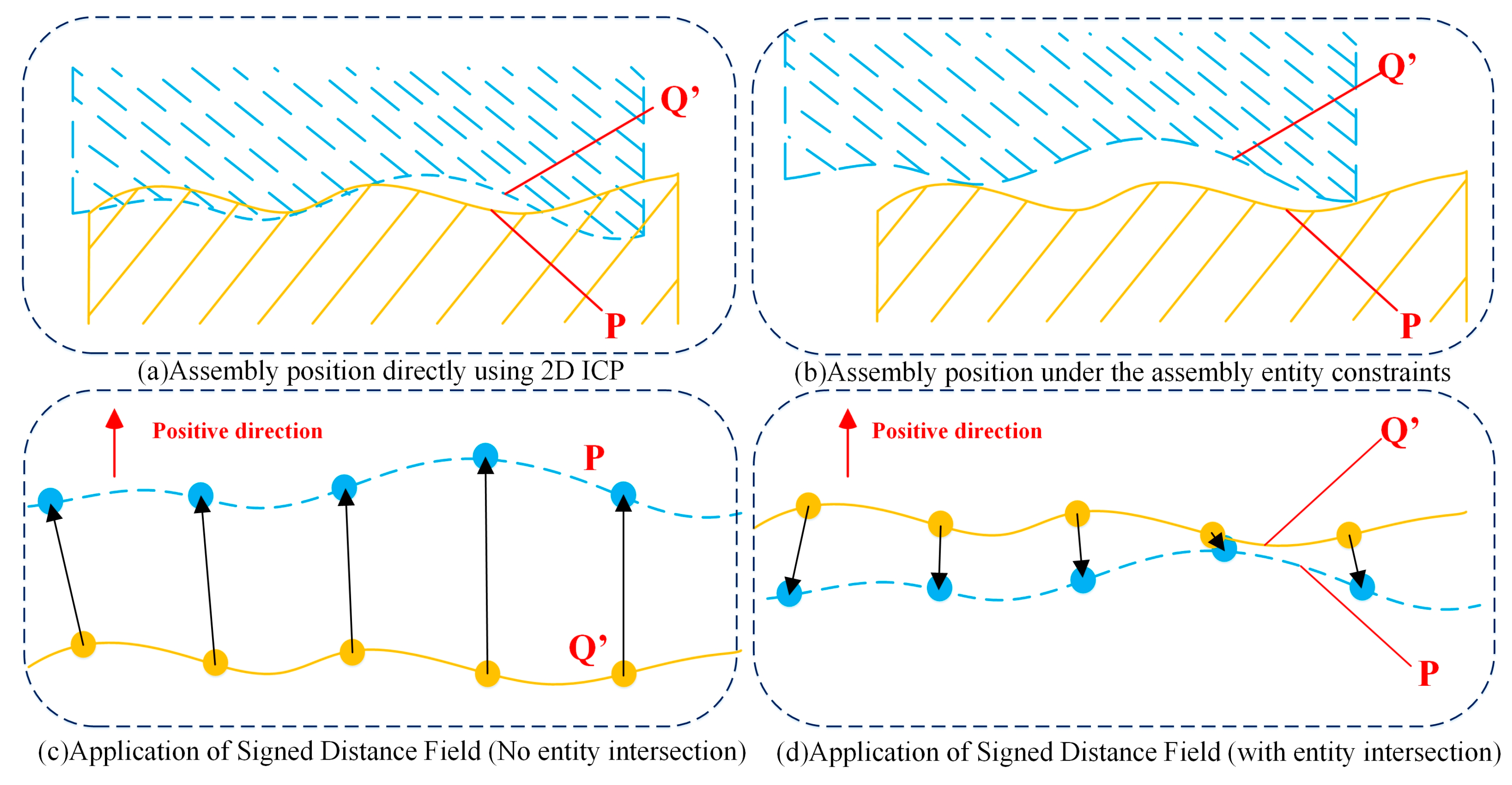
3.1. Constrained Assembly Simulation

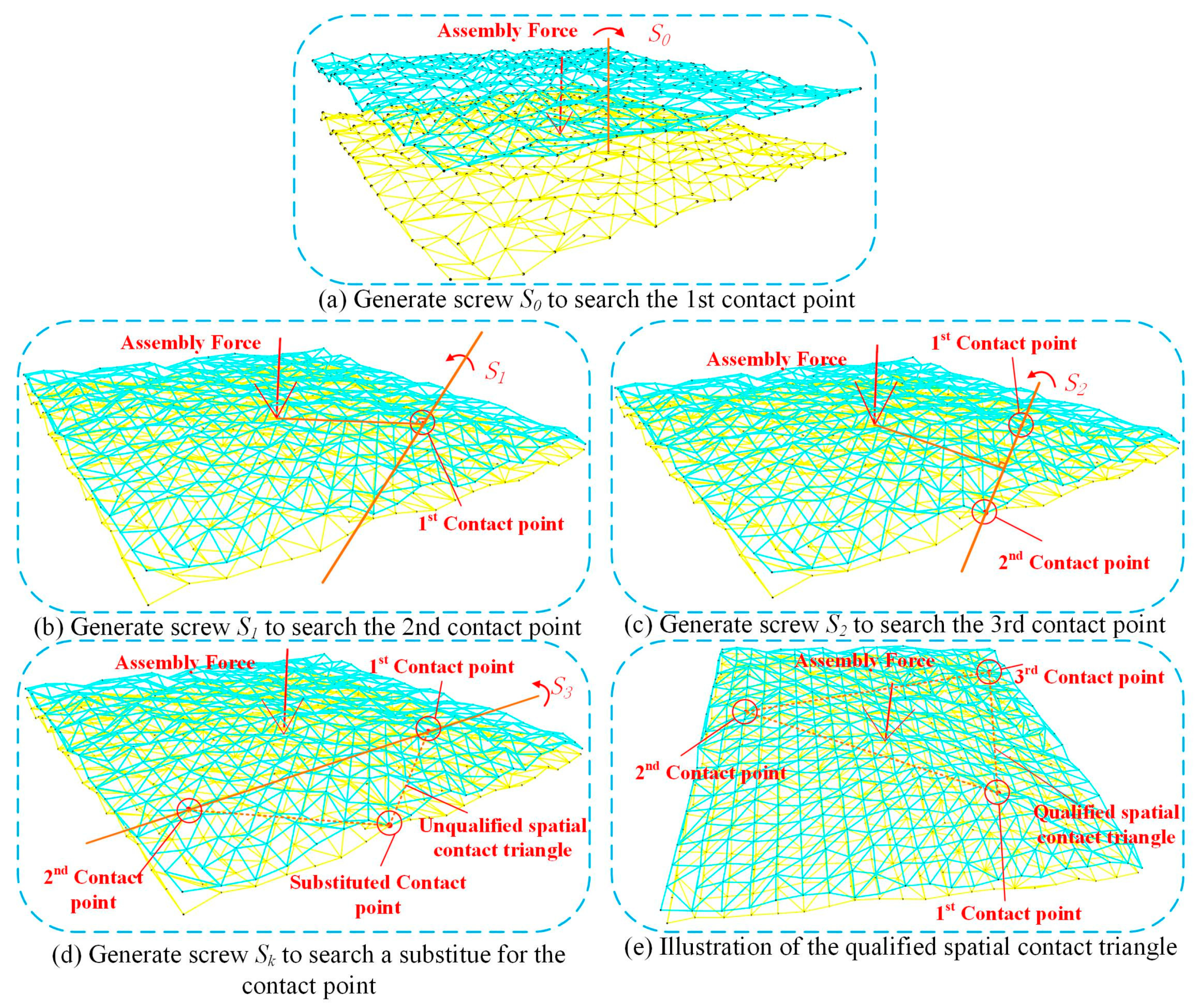
Then, the tolerance models generated by the methods described in Section 2 are used in assembly simulations. Generally, the process of assembling two parts involves the transformation of one part from its initial condition to its assembling condition, while the other part is relatively static. In this paper, the former part is called assembly part Q, and the latter part is called reference part P. The assembling transformation $\xi$ is in the form of a twist because of its splendid performance in representing the orientation, and its independence from the coordinate system transformation. Parts are considered under the geometric basis of Skin Model Shapes in this paper, which means that Q and P are in the form of meshes or point clouds. So, the assembly part Q is transformed through $\xi$ from its initial condition Q to assembling condition Q′, as shown in Equation (13):

$$Q_{\prime }=\xi ·Q$$

(13)

Twist $\xi$ is essentially an affine transformation. It can always be decomposed to a motion screw ${\xi }_i=(s_i,v_i)$ in a three-dimensional (3D) velocity vector field, containing a rotation around its axis and a translation along the axis, as shown in Equation (14):

$${\xi }_i=s_i+p_i\times v_i$$

(14)

where p_i is the vector from the spatial origin to point i. v_i is the axial velocity vector at point i. s_i is the tangential velocity vector at point i. Assembly twists of all the points of the assembly part consist the assembly transformation: $\xi =\{{\xi }_1,{\xi }_2,\cdots ,{\xi }_i,\cdots \}$.

Mathematically, Q′ is the global extremum of an object function containing Q, P, and twist $\xi$ under assembly constraints, as shown in Equation (15):

$$\xi =\arg \min (f(P,Q\prime ))$$

(15)

Choose the root mean square Euclidean distance function in Equation (16) of the closest point pairs in point clouds P and Q:

$$f=RMSED(P,Q\prime )=\text{}\sqrt{\frac{1}{n}{\displaystyle \sum _{p_i,q_i\in CPP(i)}||p_i-q_i|{|}^2}}$$

(16)

Establish the iteration object function based on Equations (13)–(16). The end condition of the iteration is the appearance of three pairs of contact points in the assembly. A pair of contact points contains a point in P and a point in Q. Furthermore, the Euclidean distance between the two points is smaller than a threshold value. Usually, using the iterative closest points (ICP) is a common method under the circumstances to find the target. However, assembly entity constraints and assembly force constraints have restricted the direct use of ICP.

Assembly entity constraints restrict the intersection of part entity in assembly simulation. As shown in Figure 2a, the direct use of ICP causes an unreasonable intersection of part materials. However, if the rule of assembly entity constraints is considered, ICP would give a result that is much more rational (in Figure 2b). A signed distance field is introduced to supervise the compliance of the assembly entity constraints. The positive direction of the signed distance field is always against the assembling direction. The signed distance vector $d_i^{sdv}(i=1,2,\cdots ,n)$ is from the points in P to the corresponding closest point in Q. When the angle between $d_i^{sdv}$ and the positive direction is under 90 degrees, $d_i^{sdv}$ is labeled positive. Otherwise, it is labeled negative. As shown in Figure 2c, all the signed distance vectors $d_i^{sdv}(i=1,2,\cdots ,n)$ are positive during iteration before assembling. However, negative signed distance vectors appear when the rule of assembly entity constraints is violated (in Figure 2d). So, the signals of $d_i^{sdv}(i=1,2,\cdots ,n)$ are repeatedly checked during the iteration.

Assembly force constraints ensure the stability of assembling conditions through restricting the location of contact points according to the assembly force. Obviously, three points provide a stable support in 3D assembly simulation, so the three contact points should not be in a line. Additionally, the assembly force vector should cross the spatial triangle made up by the three contact points. Otherwise, the current condition is unstable, and additional rotations would happen. The compliance of assembly force constraints is only checked when the iteration ends, ensuring that the final assembling state is stable. The solution of the assembling condition is decomposed into four main steps:

(1)

Compute any state of Q′ with one contact point using ICP and ensure $d_i^{sdv}>0,\forall i=1,2,\cdots ,n$ (Figure 3a). The contact point is defined as $P_1^{con}$.

(2)

Ensure $d_i^{sdv}>0,\forall i=1,2,\cdots ,n$ and search the second contact point $P_2^{con}$ using twists whose direction of $v_i$ is $\overrightarrow{P_{AF}-P_1^{con}}\times v_{AF}$ (Figure 3b), where $P_{AF}$ is the point of intersection of assembly force vector $v_{AF}$ and P.

(3)

Ensure $d_i^{sdv}>0,\forall i=1,2,\cdots ,n$ and search the third contact point $P_3^{con}$ using twists whose direction of $v_i$ is $\overrightarrow{P_1^{con}-P_2^{con}}$, as shown in Figure 3c.

(4)

Check if the current spatial contact triangle is qualified using the assembly force constraints rule: $(\overrightarrow{P_{AF}-P_1^{con}}\times \overrightarrow{P_2^{con}-P_1^{con}})·(\overrightarrow{P_{AF}-P_2^{con}}\times \overrightarrow{P_3^{con}-P_2^{con}})>0$ and $(\overrightarrow{P_{AF}-P_3^{con}}\times \overrightarrow{P_1^{con}-P_3^{con}})·(\overrightarrow{P_{AF}-P_2^{con}}\times \overrightarrow{P_3^{con}-P_2^{con}})>0$. If the conditions are not met, choose the two contact points that constitute a line closer to $P_{AF}$ (in Figure 3d) and go back to step (3). Once the conditions are met, the current condition of Q′ is the qualified assembling condition, as shown in Figure 3e.

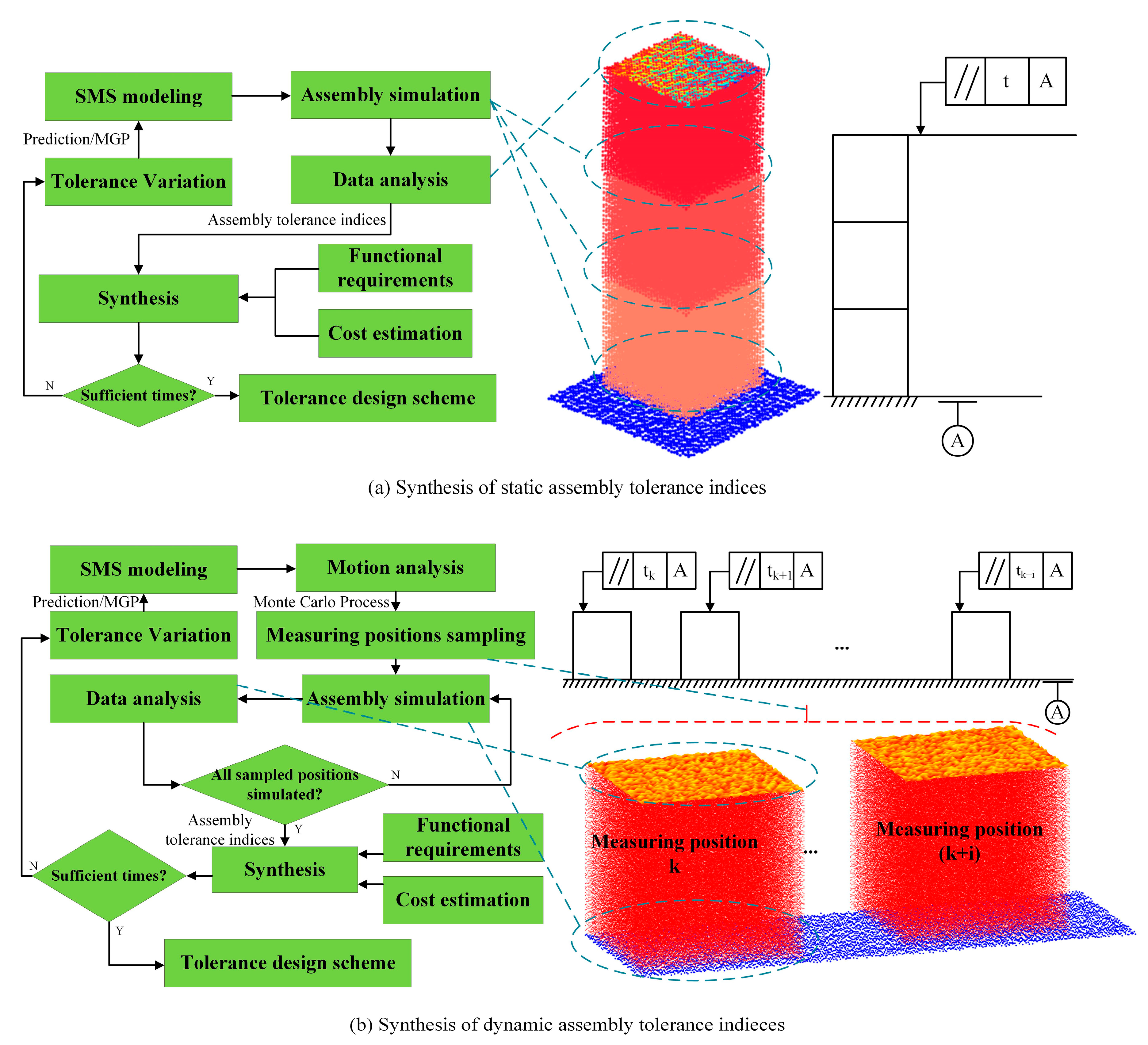
3.2. Static and Dynamic Tolerance Synthesis

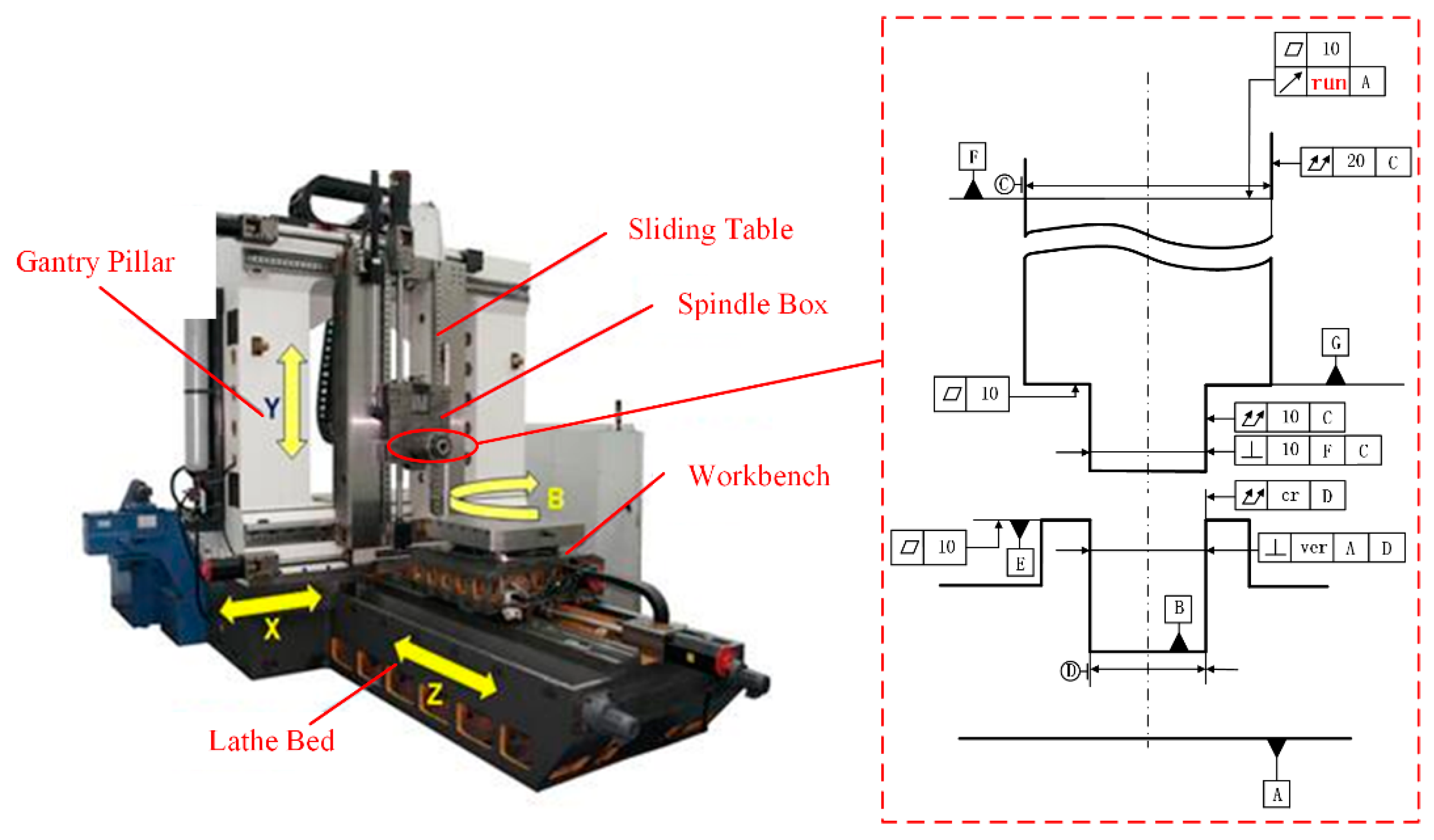
In this paper, tolerance synthesis assigns tolerance indices X, minimizes manufacturing cost, maximizes assembling probability, and meets the assembly functional requirement Y at the same time. The X tolerance index comprises the given indices X_g (mainly in outsourced parts) and to-be-designed indices X_d (mainly in self-made parts). X_g and X_d are independent from the perspective of manufacturing, but they become relevant because of the assembly functional requirement Y. Additional objectives including the manufacturing cost and assembling probability turn this issue into an optimization problem.

To increase the robustness of the design scheme, feature degradation during the machining process is considered when generating observable parts. Predictions of part surfaces at any time during the designed life are made using the methods in Section 2. Generally, surfaces in their late design age with seriously deteriorated geometric features are used in tolerance synthesis. The surfaces of predictable parts are simulated by a multivariate Gaussian process (MGP) based on given tolerance indices. Repetitive experiments and variated models are applied in the design process due to the stochastic characteristic of the MGP. Numerical experiments of assembly simulation provide assembly tolerance indices, which are usually categorized into static tolerance indices (such as verticality and parallelism) and dynamic tolerance indices (such as circular runout and end face runout). Static tolerance indices are certain indices based on measurements and the analysis of assembled Skin Model Shapes. These only vary when the tolerance models are varied (in Figure 4a). However, dynamic tolerance indices are obtained through monitoring a series of static tolerance indices by analyzing the possible motion and translational/rotational samplings. Measuring positions are sampled for experiments through a Monte Carlo process. As shown in Figure 4b, the upper end face parallelism of a sliding table on a high-precision guide is a typical dynamic tolerance index, which is calculated through a series of assembly simulations after sampling measuring positions in its translational motion. Similarly, common runout errors of cylindrical parts (such as axle parts) can also be obtained by sampling measuring orientations in the rotational motion of those parts. A small sampling interval and large sampling quantity lead to a precise estimation.

As shown in Figure 4, assembly tolerance indices are estimated through data analysis in each measuring position/orientation. The distribution of estimated assembly tolerance indices to the to-be-designed tolerance indices is summarized in the form of tables or figures. Then, an integration of assembly functional requirements and manufacturing cost estimation is introduced to outline the objectives. Due to the stochastic characteristic of tolerance models, not all the examples with the same assigned tolerance scheme can meet the assembly functional requirements. Generally, if the ratio of conformation reaches a certain threshold (such as 95%), the tolerance scheme is treated as reliable. On that basis, the manufacturing costs of all the reliable tolerance schemes are computed and compared based on industrial statistics and empirical formulation. That with the lowest costs is selected as the designed tolerance scheme.

4. Case Study

4.1. Description of the Tolerance Allocation Problem

The proposed method is applied to solve an assembly tolerance design problem in the rotary feed system of a VTM200F5 five-axis turning and milling complex center. General tolerance indices of the rotary feed system have a significant influence on the cutting precision and are extremely sensitive to geometric deviation in the cutting process due to its direct link to the cutting tool. Considering assembly tolerance, the rotary feed system is simplified to two key parts: the hole part describing devices fixing rotary bearings, and a shaft part depicting the motor spindle component. The shaft part is an outsourced part made by Ti–Al thermostable alloy with its surface specially heat-treated. So, the key accuracy indices such as location accuracy, shape accuracy, and surface accuracy should not be modified in order to protecting the special surface coating. The hole part is a self-made part made by common bearing steel. Its key accuracy indices are to be designed, as shown in Figure 5. This is a typical component containing observable parts (with the same pattern of processing features and from different batches) and predictable parts (to-be-designed parts).

In this component, the runout accuracy of the distal end of the shaft part is set as the target accuracy index due to its direct influence on the cutting accuracy. In the shaft part, the nominal flatness of the distal end surface is 0.010 mm. The nominal total runout of the distal end surface is 0.020 mm. The nominal total runout of the proximal end surface is 0.010 mm. The nominal verticality between the distal end surface and axis C is 0.010 mm. The nominal flatness of the shoulder surface is 0.010 mm. In the hole part, surface A is the assembly positioning surface. The key accuracy indices to be designed in this tolerance allocation problem are listed in

Table 1. List of the target accuracy term of the assembly, the nominal value of the accuracy terms of the shaft part, and the to-be-designed accuracy terms of the hole part.

Target Accuracy Term	Explanation	Symbol	Design Requirement
$F{R}_F$	Runout of surface F	$e_f$	0.020 mm
Accuracy Terms of the Shaft Part	Explanation	Symbol	Nominal Value
$F{L}_F$	Flatness of surface F	${\epsilon }_1$	0.010 mm
$T{R}_{C1}$	Total runout of the distal end surface	${\epsilon }_2$	0.020 mm
$T{R}_{C2}$	Total runout of the proximal end surface	${\epsilon }_3$	0.010 mm
$F{L}_G$	Flatness of shoulder surface G	${\epsilon }_4$	0.010 mm
$V{T}_{CF}$	Verticality between the distal end surface and axis C	${\epsilon }_5$	0.010 mm
Accuracy Terms of the Hole Part	Explanation	Symbol	Nominal Value
$F{L}_E$	Flatness of the shoulder surface E	$e_1$	0.010 mm
$T{R}_D$	Total runout of axis D	$e_2$	0.012 mm
$V{T}_{DA}$	Verticality between axis D and surface A	$e_3$	0.005 mm

. The flatness of the shoulder surface is FL_F. The total runout of inner hole is TR_D. The verticality between axis D and surface A is V_DA. The parallelism of the shoulder surface and surface A is PL_EA.

4.2. Stochastic Process Training and Parameter Calculation

Twenty outsourced parts were randomly chosen. Parallel lines in two directions were drawn on assembly surfaces with a uniform interval of 0.01 mm. Sampling points are defined as the intersection points of these lines. We used a non-contact coordinate measuring machine with an accuracy of at least 0.001 mm to measure the actual location of sampling points. The measured coordinates amounted to 20-point cloud sets $\{T_0,T_1,\cdots ,T_{20}\}$. Take surface F as an example: the measured point clouds sets are $\{T_{F0},T_{F1},\cdots ,T_{F20}\}$. Two of the three coordinates are determined by sampling points. The third coordinate is called the feature parameter. A first-order gradient object function of maximum likelihood estimation with weight decay is shown in Equation (17):

$$g(w)={\displaystyle \sum _{i=1}^N{\displaystyle \sum _{t=1}^T{f}_k(x_t,y_t,t)}}-{\displaystyle \sum _{i=1}^N{\displaystyle \sum _y[p(y|x,t)\times {\displaystyle \sum _{t=1}^T{f}_k(x_t,y_t,t)}]-\frac{{\displaystyle \sum w^2}}{2{\delta }^2}}}$$

(17)

Set the initial parameter weights as $w^{(0)}=\{0.1,0.1,\cdots ,0.1\}$ and the initial positive definite matrix as $M^{(0)}=diag(0.1,0.2,\cdots ,2.0)$. The coefficient of the correct term is set to 0.5. The maximum number of iterations is 1000. The feature weights of $P(y|x,t)$ corresponding to processing features are calculated according to Section 2.1. Some of the feature weights of surface F are shown in

Table 2. Value of partial feature weights of surface F.

Feature Terms	Feature Weight Value	Feature Terms	Feature Weight Value
$w_1$	0.036	$w_8$	0.124
$w_2$	0.498	$w_9$	0.965
$w_3$	0.015	$w_{10}$	2.326
$w_4$	0.968	$w_{11}$	0.216
$w_5$	1.526	$w_{12}$	2.979
$w_6$	0.732	$w_{13}$	1.521
$w_7$	1.998	$w_{14}$	1.104

.

The prediction of degraded machined surface F is obtained using the methods in Section 2.3. Consider a particular sampling point (i, j), with the assumption that its feature parameter of the location on the predictive machined surface is $y_{i,j}^{*}$ and its feature parameter of the location on the real surface is measured as $y_{i,j}^{(1)}$. The geometric average of the overall location residuals $E_r$ is set as an estimation of the precision of the predictive machined surface model, as shown in Equation (18):

$$E_r=\frac{{\displaystyle \sum _{N=1}^{20}\sqrt{{\displaystyle \sum _{i,j}{(y_{i,j}^{(N)}-{\overline{y}}_{i,j}^{(N)})}^2}}}}{{\displaystyle \sum _{N=1}^{20}\sqrt{{\displaystyle \sum _{i,j}{(y_{i,j}^{*}-y_{i,j}^{(N)})}^2}}}}$$

(18)

The value of E_r decreases when the difference between the predictive location and actual location of all the sampling points grows larger. Otherwise, the increase of E_r indicates that the predictive machined surface model is in good agreement with the real surface. Considering all the values of surface F in the 20-part samples, a comparison of the predictive machined surface using a multivariate Gaussian process and using the methodology in this paper is shown in Figure 6. Compared with the commonly used multivariate Gaussian process, the multi-dimensional Markov process provides a predictive model with higher accuracy. When time t is applied to the designed life of the assembly, the degraded machined surface near the precision failure threshold is generated and used in the assembly simulation.

4.3. Tolerance Synthesis of Example Rotary Feed Component

Numerical experiments were implemented with tolerance models of the shaft part and the hole part (in Figure 7a). Machined surface degradation prediction was combined as the model of the outsourced shaft part. Testing models for the hole part were generated based on MGP with given tolerance indices e₁, e₂, and e₃. Using the method in Section 3.1, assembling conditions and contact points were estimated based on ICP when the assembly entity constraints and assembly force constraints were checked during iterations. It is worth noting that the location of contact points varies according to the assembling contact. There are mainly three basic patterns from the perspective of the position distribution of contact points (illustrated in Figure 7a–c), which is the probability influenced by the scale of planar form errors, cylindrical form errors, and perpendicularity.

The target assembly tolerance index, the runout error e_f of surface F, was estimated by analyzing the transformed point cloud in assembling condition. A four-dimensional solution space was generated as an explanation of tolerance synthesis, constructed with e₁, e₂, and e₃ as input and e_f as an output. According to the functional requirement of the assembly, the nominal value of e_f is 0.020 mm, which means the upper limit of e_f is 0.020 mm in all the adopted tolerance schemes. However, an unnecessarily narrow tolerance interval arrangement leads to extremely high costs in fabrication and maintenance, while a combination of wide tolerance intervals causes a high ratio of assembling failure. As a result, the influence of manufacturing cost and assembly probability based on an empirical formula and experimental statistics is considered in tolerance synthesis. Assembly examples with acquired functional requirements are called “successful” assemblies. Assembling probability is estimated by the proportion of successful assemblies of all the experimental assemblies. According to industrial practice, a yield rate of 95% is accepted, which means that the assembling probability should be more than 95%. The region of interest in the solution space is generated following this rule.

The empirical relationship between the tolerance interval and manufacturing cost based on historical industrial practice is shown in Equation (19), where ${\alpha }_1$, ${\alpha }_2$, and ${\alpha }_3$ are manufacturing difficulty coefficients, and K is a scaling factor:

$$C=K(\frac{{\alpha }_1}{e_1^2}+\frac{{\alpha }_2}{e_2^2}+\frac{{\alpha }_3}{e_3^2}）$$

(19)

The influences of e₁, e₂, and e₃ on the assembly probability and manufacturing cost are shown in Figure 8a. A Monte Carlo sampling method was applied in the four-dimensional solution space to calculate the output of all the sampled inputs. High-density sampling was conducted in the region of interest to ensure searching accuracy; the density of sampling points was lower, but even outside the region of interest, it avoided falling into the local optimum. The top 1% with the lowest manufacturing cost was approximately fitted into an ellipsoid limit surface, as shown in Figure 8b, where the axes of e₁, e₂, and e₃ are even, and the axis of e_f is uneven.

Three examples with the lower manufacturing cost and satisfactory assembling probability constitute the designed tolerance scheme, as shown in

Table 3. Design requirement of the object tolerance term and the nominal and designed value of the to-be-designed tolerance terms.

Objective Tolerance Term	${\mathit{e}}_{\mathit{f}}$	Assembly Functional Requirement		${\mathit{e}}_{\mathit{f}}\le 0.020$
To-be-designed tolerance terms	$e_1$	$e_2$	$e_3$	Assembling probability	Relative manufacturing cost
Nominal value (mm)	0.010	0.012	0.005	1	1
Designed scheme 1 (mm)	0.013	0.016	0.009	0.957	0.644
Designed scheme 2 (mm)	0.012	0.014	0.016	0.959	0.679
Designed scheme 3 (mm)	0.014	0.015	0.006	0.969	0.754

. The designed scheme with an assembling probability larger than 95% and the lowest manufacturing cost is listed in bold. The designed value of all three to-be-designed tolerance terms e₁, e₂, and e₃ were enlarged by 0.003, 0.004, and 0.004, respectively. The objective functional requirement was still met, and the assembling probability was satisfactory. However, the expansion of the tolerance interval caused a 35.6% reduction of the manufacturing cost. The other two listed example designed schemes can also be considered depending on the acceptable manufacturing cost considered.

5. Conclusions

A tolerance design method based on Skin Model Shapes considering processing feature degradation is proposed in this paper. To include the geometric form deviation and degrading processing feature, the machined surface model was constructed in the form of 3D point clouds based on Skin Model Shapes. A uniform sampling was implemented on the grid nodes of the assembly surface. Using machine part samples in mass production, the point dataset was acquired by a high-precision coordinate measuring machine. Then, a continuous-time multi-dimensional Markov process was trained to model the feature degradation process; it was also used in further numerical experiments. To improve the reliability and rationality of the numerical experiments, the assembly force constraints and assembly entity constraints were applied to the assembly simulation. Then, the static and dynamic tolerance indices were analyzed and synthesized. The values of the to-be-designed tolerance terms were designed with the aim of conforming to the assembly tolerance requirement, guaranteeing the assembling probability and reducing the manufacturing cost as much as possible.

The tolerance design method in this paper was applied to an example assembly tolerance design problem regarding a five-axis machine tool rotary feed system. Data analysis indicated that the predictive machined surface model is more accurate than that employed in common Skin Model Shape methods. The designed tolerance scheme has a larger tolerance interval and lower manufacturing costs. That is, the generation of the feature degradation model comprises an in-depth profile and dynamic investigation for production systems based on sampling machining data, which improved the ability of self-configuration of the designed tolerance scheme. Also, the designing reliability and robustness was improved through the improved assembly simulation considering multiple assembling constraints. In addition, the collection and analysis of the manufacturing information and the process of virtual simulation is closely related to the deployment of Internet of Things (IoT) systems and Cyber-Physical Production Systems (CPPS), especially manufacturing equipment with sensors, automation, and information flow. As a result, the proposed method helps to promote the design capability and production flexibility, and improves competence in an increasingly competitive business environment. It provides a new way to design with digitality and intelligence to help fill in the gaps between virtual engineering processes and virtual engineering factories, which would contribute to completing the structure of Industry 4.0. However, evenly distributed sampling points on the assembly surface may cause model distortion when local geometric features are complicated. Boundary treatment in point cloud combination, advanced sampling methods, and dimensionality reduction in solution space also need attention in further research.

References

1. Erboz, G. How to define industry 4.0: The main pillars of industry 4.0. In Proceedings of the 7th International Conference on Management (ICoM 2017), Nitra, Slovakia, 1–2 June 2017. [Google Scholar]
2. Hofmann, E.; Rüsch, M. Industry 4.0 and the current status as well as future prospects on logistics. Comput. Ind. 2017, 89, 23–34. [Google Scholar] [CrossRef]
3. Lu, Y. Industry 4.0: A survey on technologies, applications and open research issues. J. Ind. Inf. Integr. 2017, 6, 1–10. [Google Scholar] [CrossRef]
4. Geetha, K. Tolerance allocation and scheduling for complex assembly. Int. J. Appl. Eng. Res. 2015, 10, 4000–4003. [Google Scholar]
5. Shoukr, D.S.L.; Gadallah, M.H.; Metwalli, S.M. The reduced tolerance allocation problem. In Proceedings of the ASME’s International Mechanical Engineering Congress and Exposition (IMECE2016), Phoenix, AZ, USA, 11–17 November 2016. [Google Scholar]
6. Khodaygan, S. Meta-model based multi-objective optimisation method for computer-aided tolerance design of compliant assemblies. Int. J. Comput. Integr. Manuf. 2019, 32, 27–42. [Google Scholar] [CrossRef]
7. Delos, V.; Arroyave-Tobón, S.; Teissandier, D. Introducing a projection-based method to compare three approaches computing the accumulation of geometric variations. In Proceedings of the ASME 2018 International Design Engineering Technical Conferences and Computers and Information in Engineering Conference, Quebec City, QC, Canada, 26–29 August 2018. [Google Scholar]
8. Lin, E.E.; Zhang, H.C. Theoretical tolerance stackup analysis based on tolerance zone analysis. Int. J. Adv. Manuf. Technol. 2001, 17, 257–262. [Google Scholar] [CrossRef]
9. Wang, Y. Closed-loop analysis in semantic tolerance modeling. J. Mech. Des. 2008, 130, 061701. [Google Scholar] [CrossRef]
10. Geis, A.; Husung, S.; Oberänder, A.; Weber, C.; Adam, J. Use of vectorial tolerances for direct representation and analysis in CAD-systems. Proc. CIRP 2015, 27, 230–240. [Google Scholar] [CrossRef]
11. Heling, B.; Aschenbrenner, A.; Walter, M.S.J.; Wartzack, S. On connected tolerances in statistical tolerance-cost-optimization of assemblies with interrelated dimension chains. Proc. CIRP 2016, 43, 262–267. [Google Scholar] [CrossRef]
12. Ameta, G.; Davidson, J.K.; Shah, J.J. Tolerance-maps applied to a point-line cluster of features. J. Mech. Des. 2007, 129, 782–792. [Google Scholar] [CrossRef]
13. Bhide, S.; Ameta, G.; Davidson, J.K.; Shah, J.J. Tolerance-maps applied to the straightness and orientation of an axis. In Models for Computer Aided Tolerancing in Design and Manufacturing; Springer: Dordrecht, The Netherlands, 2007. [Google Scholar]
14. Chitale, A.N.; Davidson, J.K.; Shah, J.J. Statistical tolerance analysis with sensitivities established from tolerance-maps and deviation spaces. J. Comput. Inf. Sci. Eng. 2019, 19, 041002. [Google Scholar] [CrossRef]
15. Cheng, H.; Li, Y.; Zhang, K.F.; Su, J. Bin Efficient method of positioning error analysis for aeronautical thin-walled structures multi-state riveting. Int. J. Adv. Manuf. Technol. 2011, 55, 217–233. [Google Scholar] [CrossRef]
16. 1Wang, H.; Liu, J. Tolerance simulation of thin-walled c-section composite beam assembling with small displacement torsor model. Proc. CIRP 2016, 43, 274–279. [Google Scholar]
17. Li, H.; Zhu, H.; Zhou, X.; Li, P.; Yu, Z. A new computer-aided tolerance analysis and optimization framework for assembling processes using DP-SDT theory. Int. J. Adv. Manuf. Technol. 2016, 86, 1299–1310. [Google Scholar] [CrossRef]
18. Du, Q.; Zhai, X.; Wen, Q. Study of the ultimate error of the axis tolerance feature and its pose decoupling based on an area coordinate system. Appl. Sci. 2018, 8, 435. [Google Scholar] [CrossRef]
19. Yan, H.; Cao, Y.; Yang, J. Statistical tolerance analysis based on good point set and homogeneous transform matrix. Proc. CIRP 2016, 43, 178–183. [Google Scholar] [CrossRef]
20. Laperrière, L.; Elmaraghy, H.A. Tolerance analysis and synthesis using Jacobian transforms. CIRP Ann. 2000, 49, 359–362. [Google Scholar] [CrossRef]
21. Desrochers, A.; Ghie, W.; Laperrière, L. Application of a unified jacobian—Torsor model for tolerance analysis. J. Comput. Inf. Sci. Eng. 2003, 3, 2–14. [Google Scholar] [CrossRef]
22. Zeng, W.; Rao, Y.; Wang, P.; Yi, W. A solution of worst-case tolerance analysis for partial parallel chains based on the Unified Jacobian-Torsor model. Precis. Eng. 2017, 47, 276–291. [Google Scholar] [CrossRef]
23. Kopardekar, P.; Anand, S. Tolerance allocation using neural networks. Int. J. Adv. Manuf. Technol. 1995, 10, 269–276. [Google Scholar] [CrossRef]
24. Luo, C.; Franciosa, P.; Ceglarek, D.; Ni, Z.; Jia, F. A novel geometric tolerance modeling inspired by parametric space envelope. IEEE Trans. Autom. Sci. Eng. 2018, 15, 1386–1398. [Google Scholar] [CrossRef]
25. Samper, S.; Formosa, F. Form Defects tolerancing by natural modes analysis. J. Comput. Inf. Sci. Eng. 2007, 7, 44–51. [Google Scholar] [CrossRef]
26. Homri, L.; Goka, E.; Levasseur, G.; Dantan, J.Y. Tolerance analysis—Form defects modeling and simulation by modal decomposition and optimization. CAD Comput. Aided Des. 2017, 91, 46–59. [Google Scholar] [CrossRef]
27. Lin, E.E. Graph-Matrix-Based Automated Tolerance Analysis and Setup Planning in Computer-Aided Process Planning. Ph.D. Thesis, Texas Tech University, Lubbock, TX, USA, 2000. [Google Scholar]
28. Zhang, K.; Li, Y.; Tang, S. An integrated modeling method of unified tolerance representation for mechanical product. Int. J. Adv. Manuf. Technol. 2010, 46, 217–226. [Google Scholar] [CrossRef]
29. Schleich, B.; Wartzack, S.; Anwer, N.; Mathieu, L. Skin model shapes: Offering new potentials for modelling product shape variability. In Proceedings of the ASME 2015 International Design Engineering Technical Conferences and Computers and Information in Engineering Conference, Boston, MA, USA, 2–5 August 2015. [Google Scholar]
30. ISO 17450-1. Geometrical Product Specifications (GPS): General Concepts: Part 1: Model for Geometrical Specification and Verification; ISO: Geneva, Switzerland, 2011. [Google Scholar]
31. ISO 17450-2. Geometrical Product Specifications (GPS)—General Concepts: Part 2: Basic Tenets, Specifications, Operators, Uncertainties and Ambiguities; ISO: Geneva, Switzerland, 2012. [Google Scholar]
32. Ballu, A.; Mathieu, L. Univocal expression of functional and geometrical tolerances for design, manufacturing and inspection. In Computer-Aided Tolerancing; Springer: Dordrecht, The Netherlands, 2011. [Google Scholar]
33. Anwer, N.; Ballu, A.; Mathieu, L. The skin model, a comprehensive geometric model for engineering design. CIRP Ann. Manuf. Technol. 2013, 62, 143–146. [Google Scholar] [CrossRef]
34. Zhang, M.; Anwer, N.; Mathieu, L.; Zhao, H. A discrete geometry framework for geometrical product specifications. In Proceedings of the 21st CIRP Design Conference, Kaist, Korea, 1 January 2011. [Google Scholar]
35. Schleich, B.; Anwer, N.; Mathieu, L.; Wartzack, S. Skin Model Shapes: A new paradigm shift for geometric variations modelling in mechanical engineering. CAD Comput. Aided Des. 2014, 50, 1–15. [Google Scholar] [CrossRef]
36. Yacob, F.; Semere, D.; Nordgren, E. Octree-based generation and variation analysis of skin model shapes. J. Manuf. Mater. Process. 2018, 2, 52. [Google Scholar] [CrossRef]
37. Yan, X.; Ballu, A. Generation of consistent skin model shape based on FEA method. Int. J. Adv. Manuf. Technol. 2017, 92, 789–802. [Google Scholar] [CrossRef]
38. Schleich, B.; Anwer, N.; Mathieu, L.; Wartzack, S. Contact and mobility simulation for mechanical assemblies based on skin model shapes. J. Comput. Inf. Sci. Eng. 2015, 15, 021009. [Google Scholar] [CrossRef]
39. Dantan, J.-Y. Comparison of skin model representations and tooth contact analysis techniques for gear tolerance analysis. J. Comput. Inf. Sci. Eng. 2015, 15, 021010. [Google Scholar] [CrossRef]
40. Yan, X. Assembly Simulation and Evaluation Based on Generation of Virtual Workpiece with Form Defect. Ph.D. Thesis, Université de Bordeaux, Bordeaux, France, 2018. [Google Scholar]
41. Wang, J.; Sanchez, J.; Iturrioz, J.; Ayesta, I. Geometrical defect detection in the wire electrical discharge machining of fir-tree slots using deep learning techniques. Appl. Sci. 2018, 9, 90. [Google Scholar] [CrossRef]
42. Sun, J.; Rahman, M.; Wong, Y.S.; Hong, G.S. Multiclassification of tool wear with support vector machine by manufacturing loss consideration. Int. J. Mach. Tools Manuf. 2004, 44, 1179–1187. [Google Scholar] [CrossRef]
43. Dai, W.; Chi, Y.; Lu, Z.; Wang, M.; Zhao, Y. Research on reliability assessment of mechanical equipment based on the performance–feature model. Appl. Sci. 2018, 8, 1619. [Google Scholar] [CrossRef]
44. Ozcelik, B.; Bayramoglu, M. The statistical modeling of surface roughness in high-speed flat end milling. Int. J. Mach. Tools Manuf. 2006, 46, 1395–1402. [Google Scholar] [CrossRef]
45. Shu, M.H.; Hsu, B.M.; Kapur, K.C. Dynamic performance measures for tools with multi-state wear processes and their applications for tool design and selection. Int. J. Prod. Res. 2010, 48, 4725–4744. [Google Scholar] [CrossRef]
46. Hsu, B.M.; Shu, M.H.; Wu, L. Dynamic performance modelling and measuring for machine tools with continuous-state wear processes. Int. J. Prod. Res. 2013, 51, 4718–4731. [Google Scholar] [CrossRef]
47. Moghaddass, R.; Zuo, M.J. A parameter estimation method for a condition-monitored device under multi-state deterioration. Reliab. Eng. Syst. Saf. 2012, 106, 94–103. [Google Scholar] [CrossRef]
48. Cannarile, F.; Compare, M.; Baraldi, P.; Di Maio, F.; Zio, E. Homogeneous continuous-time, finite-state hidden semi-markov modeling for enhancing empirical classification system diagnostics of industrial components. Machines 2018, 6, 34. [Google Scholar] [CrossRef]
Figure 1. Temporal and spatial Markov properties of planar machining surface (a), and an illustration of the precision state degradation in the production sequence (b,c).
Applsci 09 03216 g001
Figure 2. Illustration of assembly entity constraints and the application of a signed distance field in realizing the rule.
Applsci 09 03216 g002
Figure 3. Main steps in the computation of assembling condition when considering assembly force constraints.
Applsci 09 03216 g003
Figure 4. Synthesis of static and dynamic assembly tolerance indices based on assembly simulation.
Applsci 09 03216 g004
Figure 5. An assembly tolerance design example in designing the rotary feed system of a five-axis turning and milling complex center (VTM200F5).
Applsci 09 03216 g005
Figure 6. Comparison of overall location residuals of the predictive machined surface using the multivariate Gaussian process and using the method proposed in this paper.
Applsci 09 03216 g006
Figure 7. Numerical experiments (a) and three basic patterns of contact point positions (bd).
Applsci 09 03216 g007
Figure 8. Distribution of assembly probability and manufacturing cost (a), and solution searching in a four-dimensional solution space constructed by even axes of e1, e2, and e3, and the uneven axis of ef (b).
Applsci 09 03216 g008