Detecting and Learning Unknown Fault States by Automatically Finding the Optimal Number of Clusters for Online Bearing Fault Diagnosis


Abstract
:Featured Application
Abstract
1. Introduction
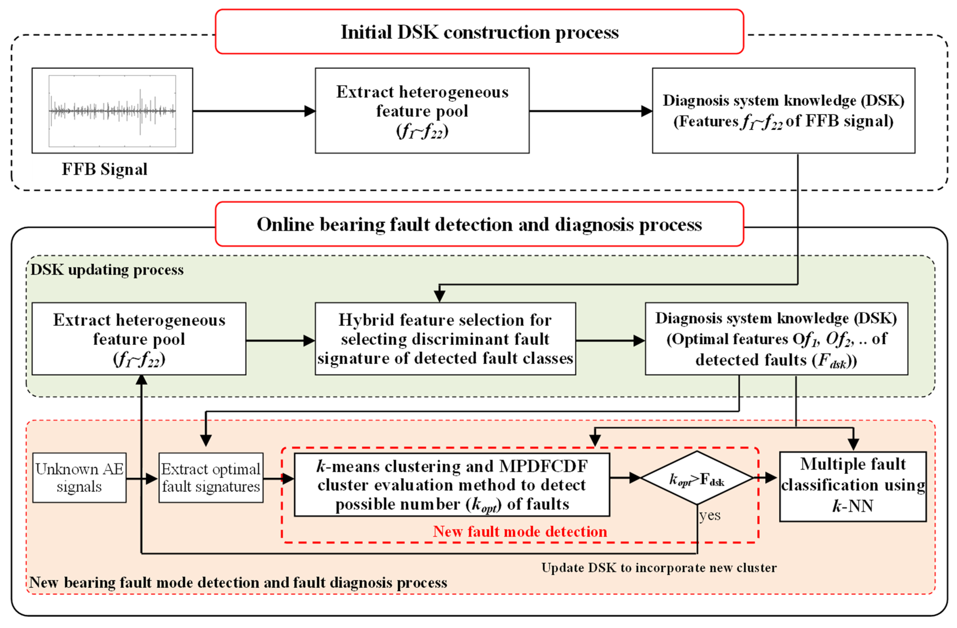
- Since it is difficult to know in advance what types of faults a healthy bearing can experience, traditional offline fault diagnosis systems classify faults on the basis of incomplete knowledge. To address this issue, we propose an online bearing fault diagnosis model that first detects unknown fault modes in real-time using k-means clustering and continually updates the DSK for more reliable fault diagnosis.
- It is difficult to determine the number of discernible fault modes through k-means clustering alone without knowing how to define kkmean. To address this issue, we propose a new cluster evaluation method, the MPDFCDF, to identify the optimal number of clusters (kopt) in the fault signatures.
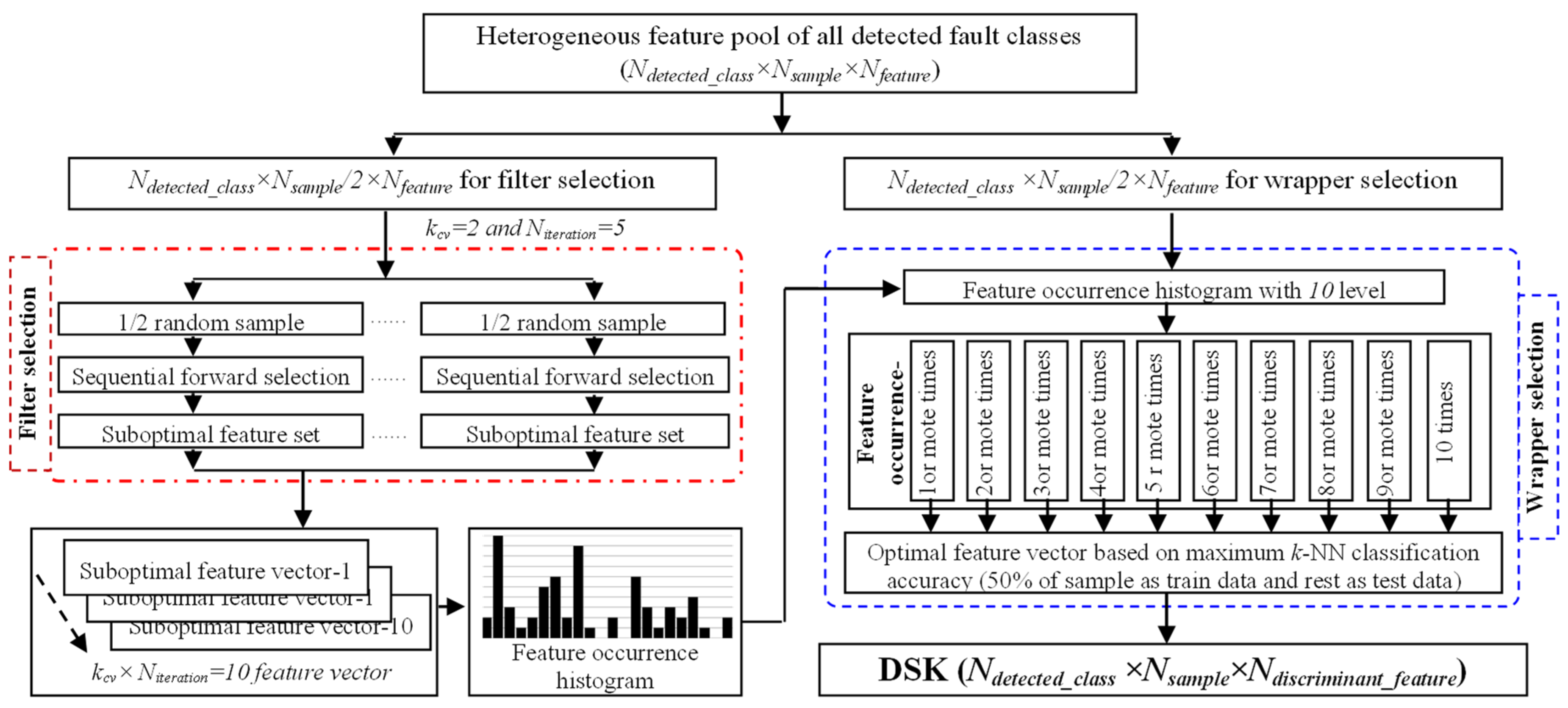
- To evaluate our proposed model, we recorded bearing signals for different shaft speeds and constructed a heterogeneous fault signatures pool to extract the maximum possible fault information. We used a hybrid fault signature selection to create discriminative fault signatures and build a DSK. Finally, we used the k-NN classification algorithm to estimate the classification performance.
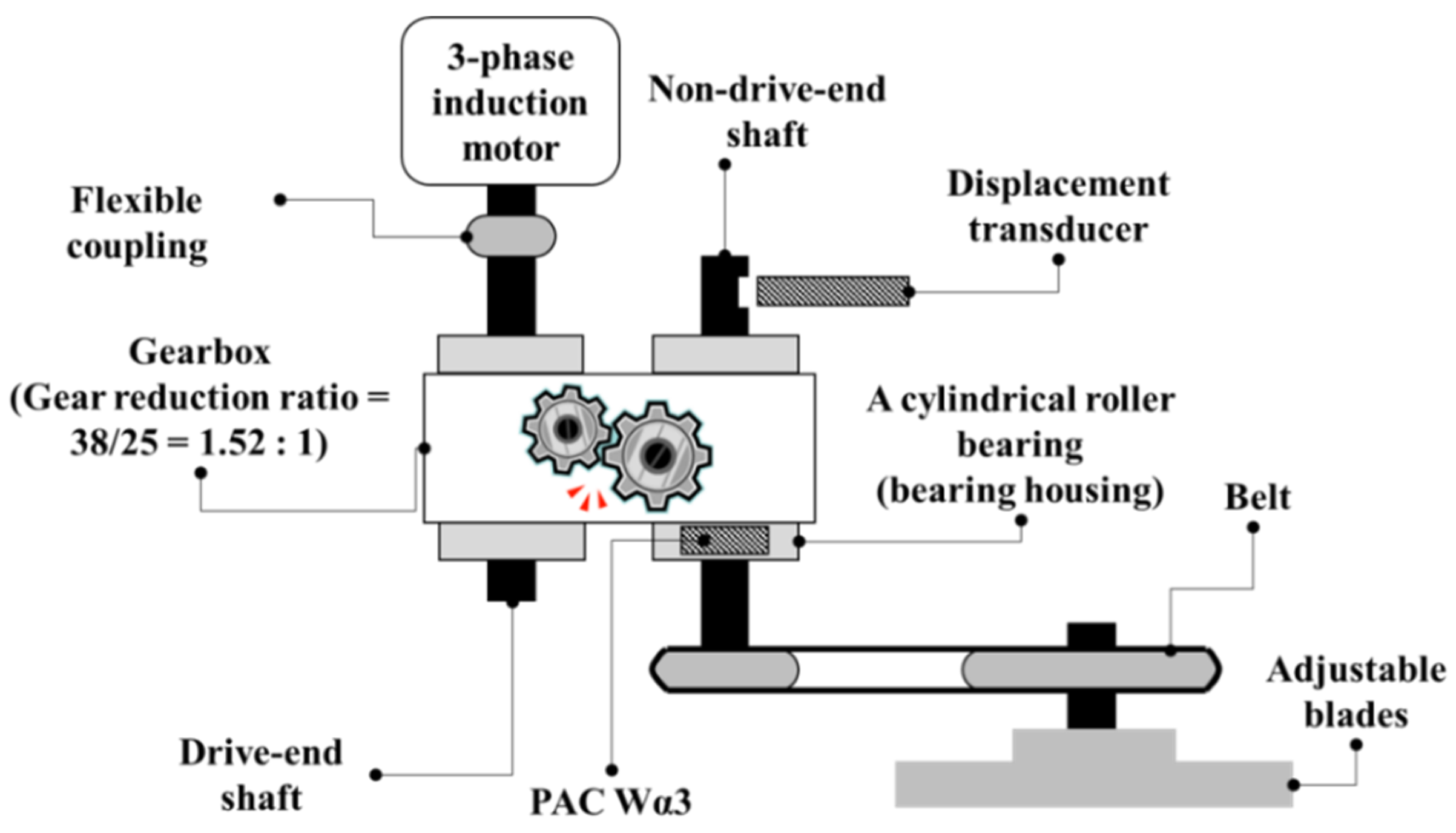
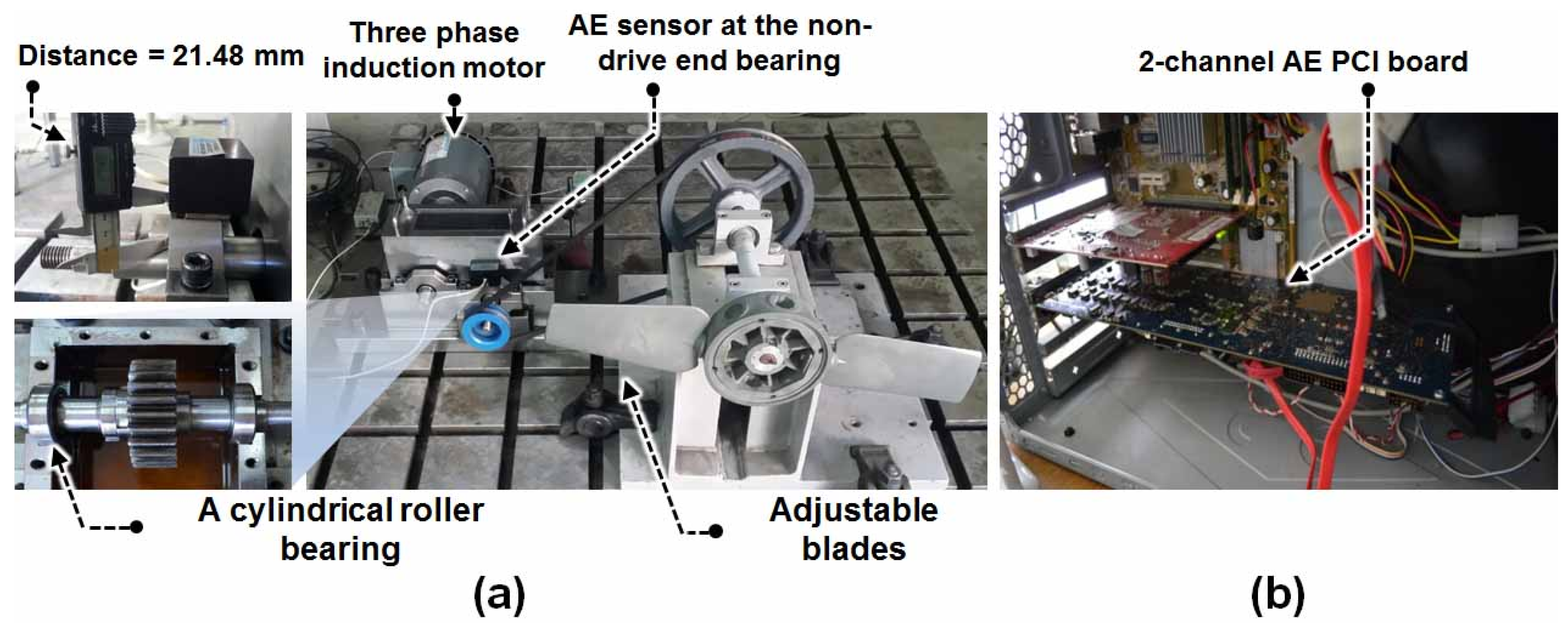
2. Data Acquisition
3. Proposed Online Fault Diagnosis Model
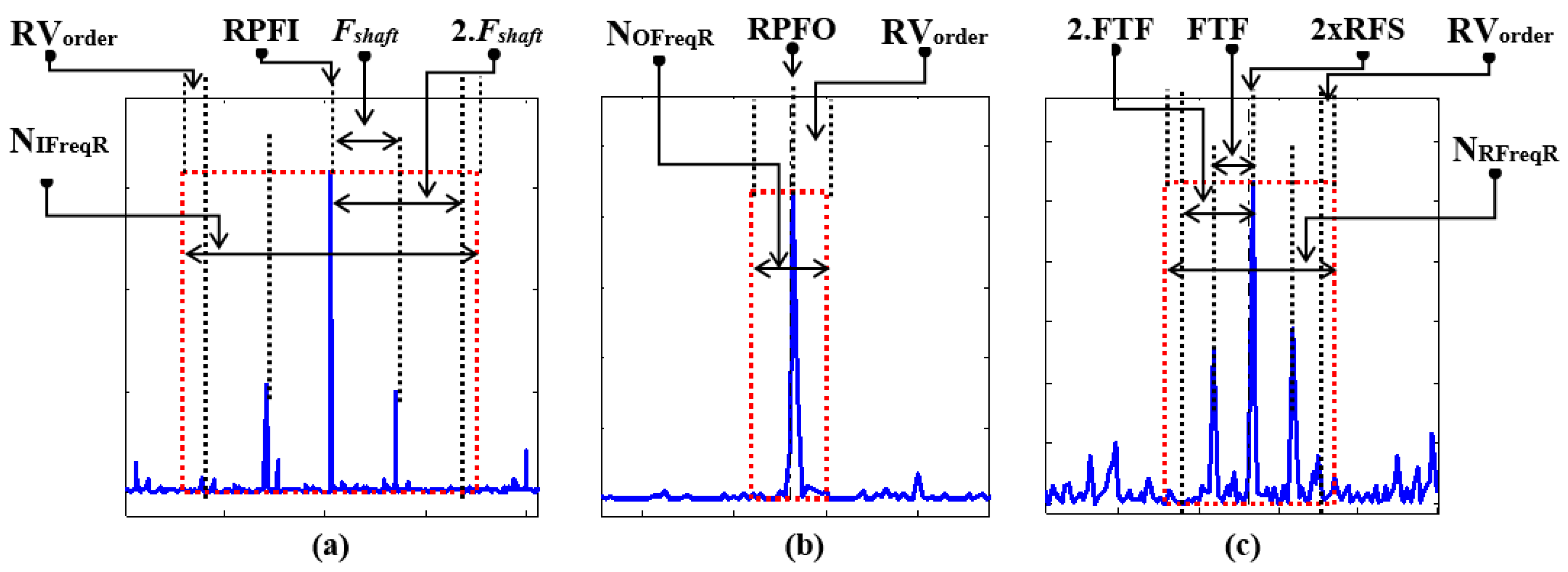
3.1. Heterogeneous Feature Pool Configuration
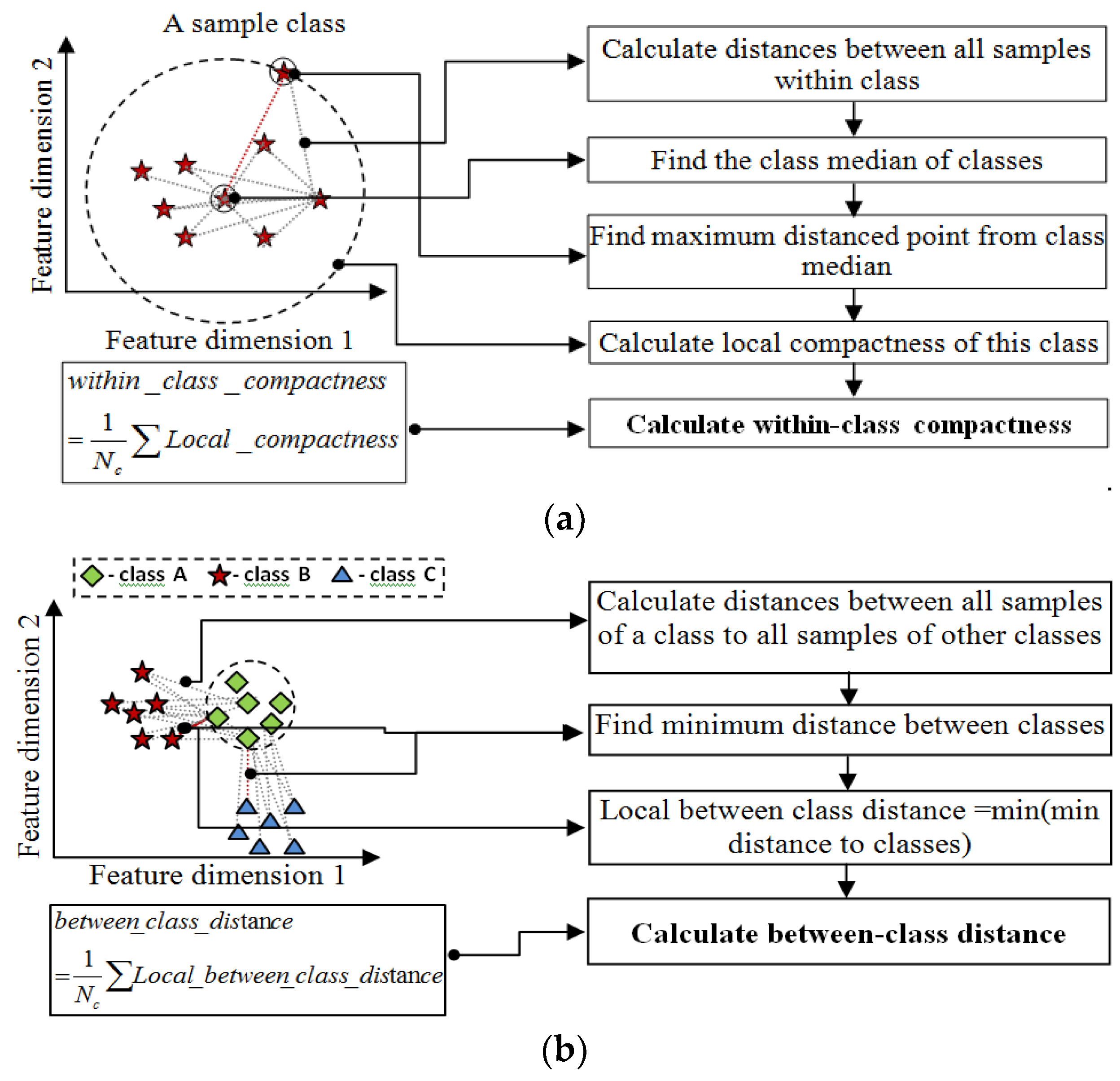
3.2. DSK Construction by Selecting Discriminant Fault Signatures of Detected Fault Modes
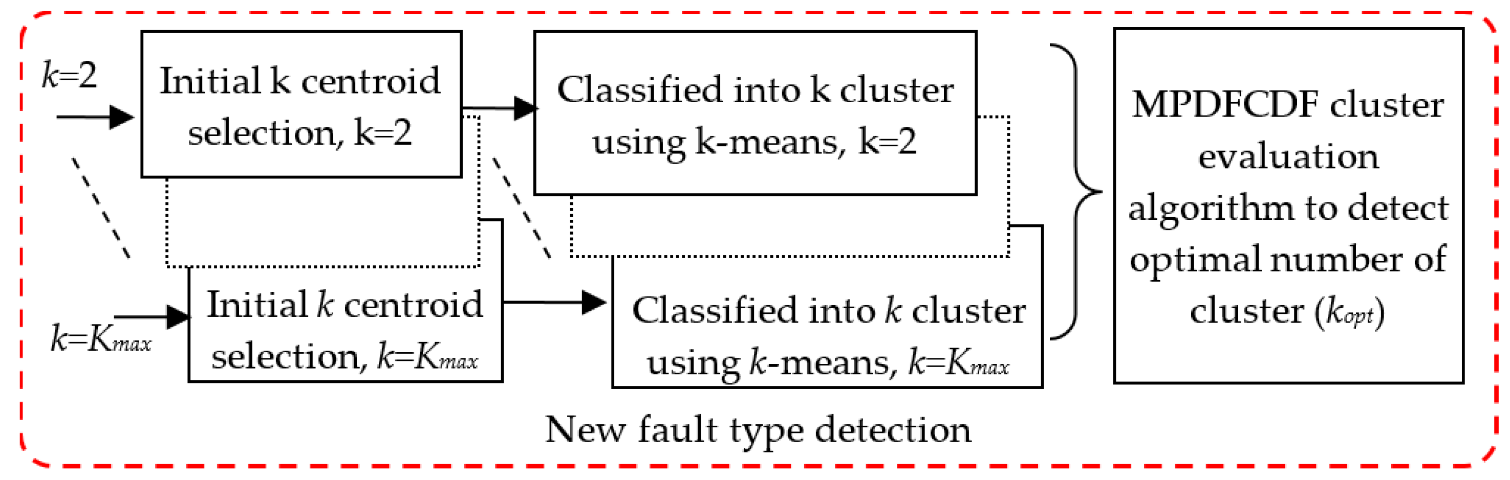
3.3. Proposed New Fault Mode Detection
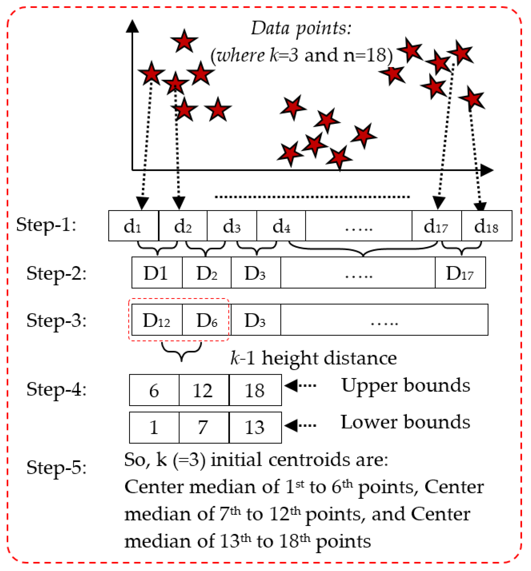
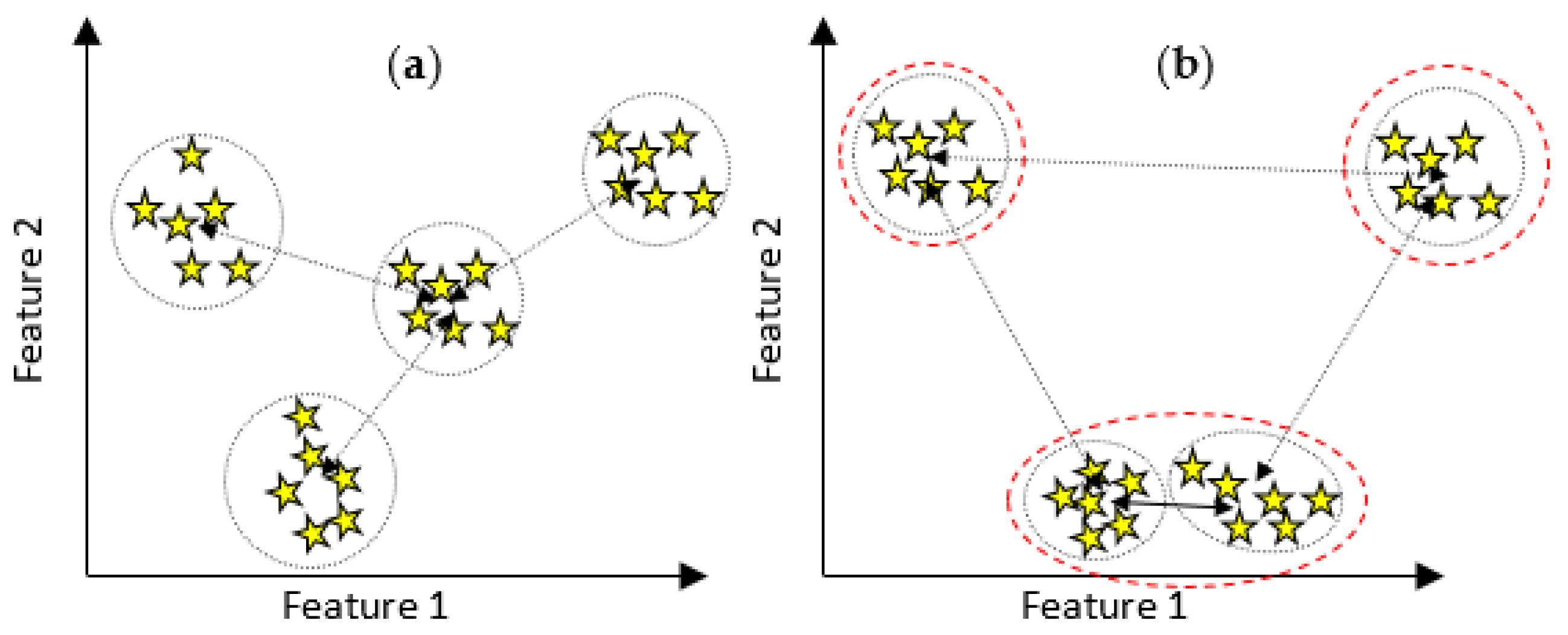
3.3.1. k-Means Clustering
3.3.2. The Proposed MPDFCDF Cluster Evaluation Method
- Step 1: Classify samples belonging to k clusters by k-means clustering;
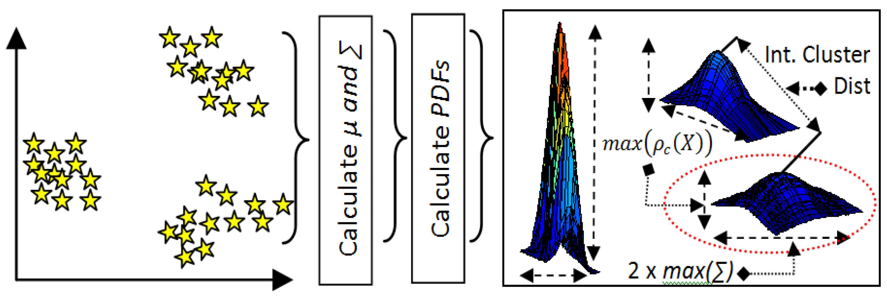
- Step 2: Calculate the mean µ and covariance ∑ of all clusters;
- Step 3: Calculate the PDFs for all clusters using Equation (8);
- Step 4: Calculate the local distribution factor for each cluster;the 2-sigma rule [41] is used here, which states that 95% of samples exist within 2-sigma of the mean and the remaining 5% can be regarded as outliers.
- Step 5: Calculate the global density factor for the distributionGlobal Density Factor = min(Local_density_factor);
- Step 6: Calculate the global separability factorwhereGlobal Separability Factor = min(Inter_Cluster_Dist)
- Step 7: Calculate the MPDFCDFwhere the minimum MPDFCDF value identifies kopt.MPDFCDF = abs(Global Density Factor-Global Separability Factor)
3.4. System Update
3.5. Fault Classification Using k-NN
4. Experimental Results and Analysis
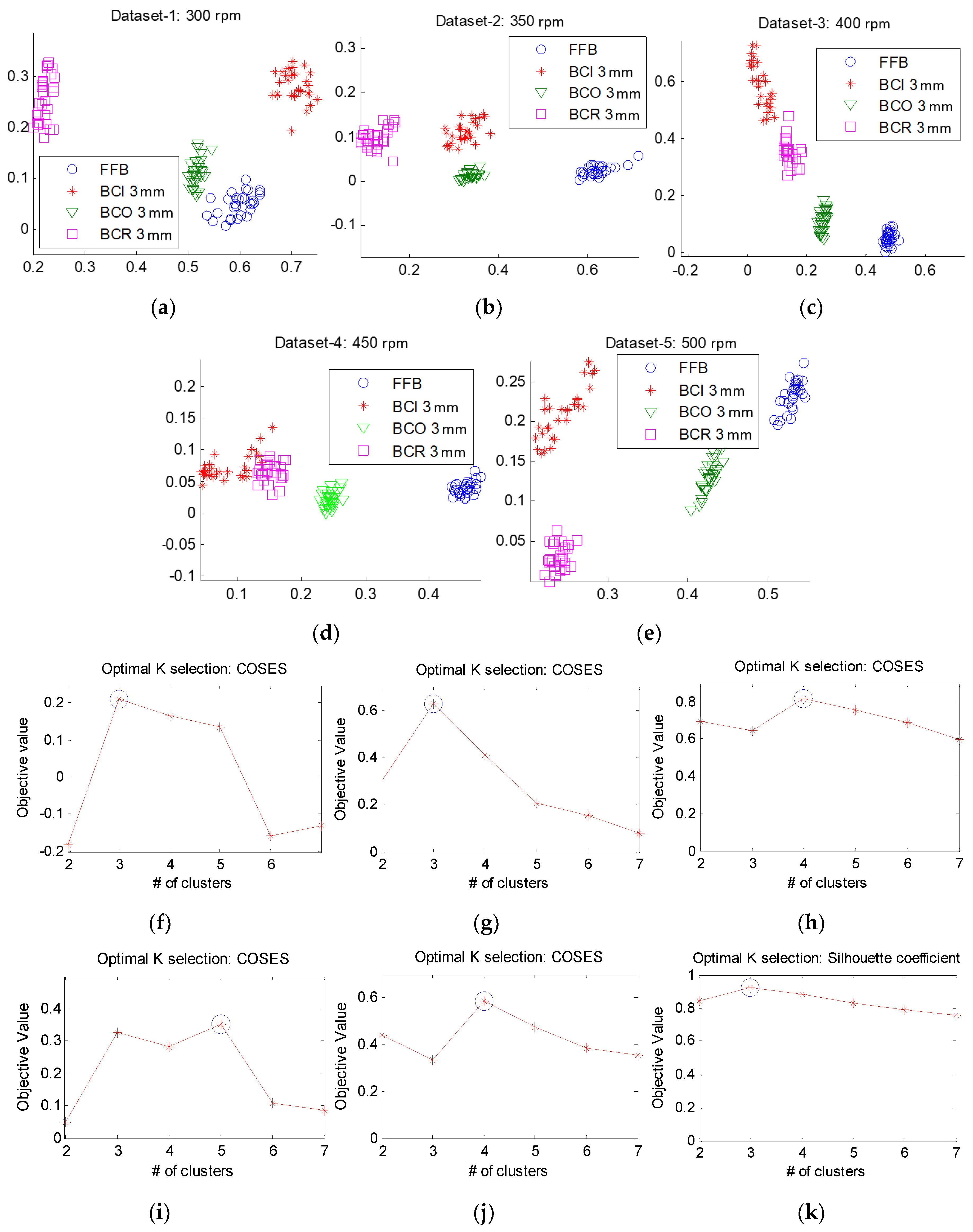
4.1. Experimental Datasets
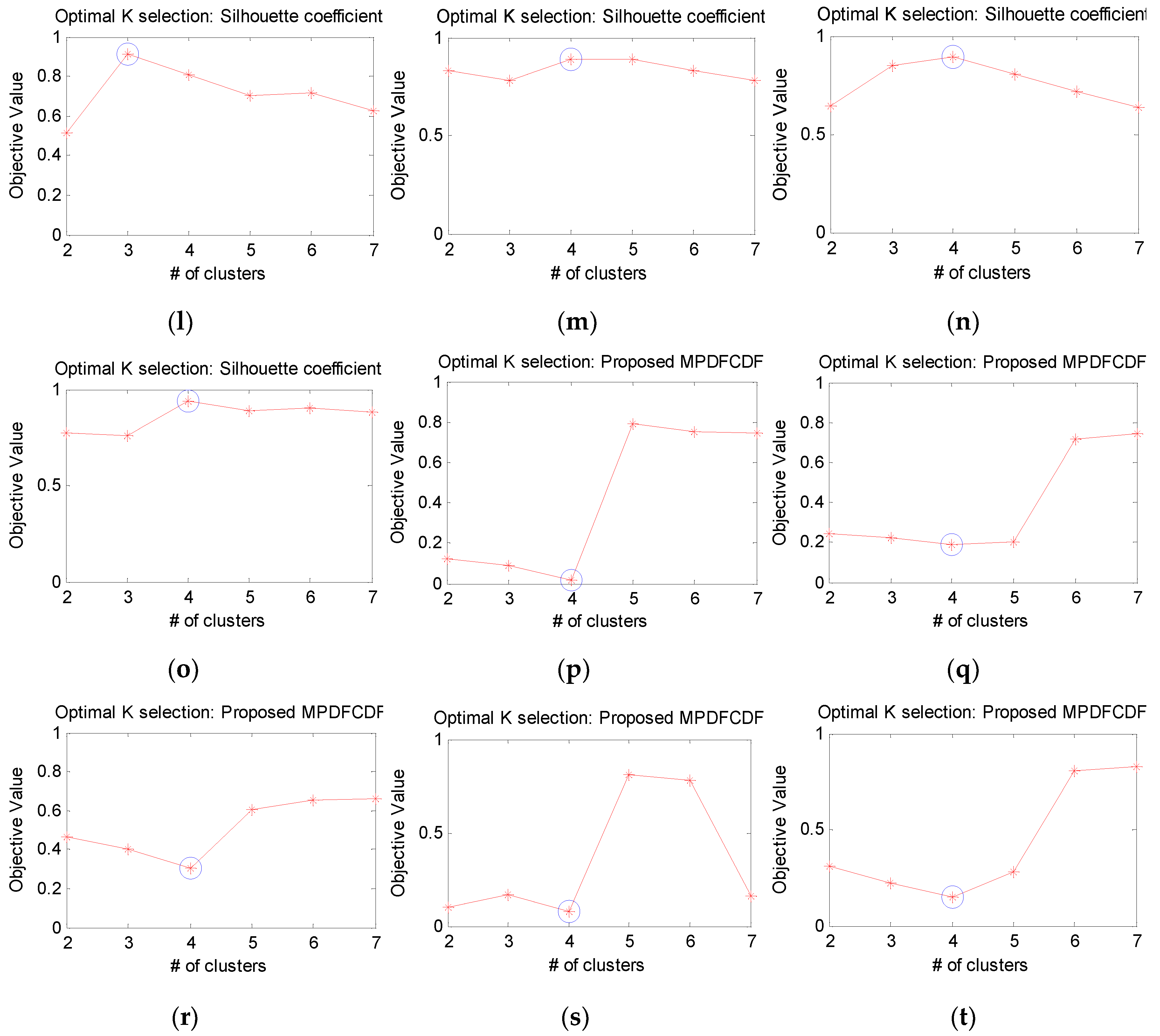
4.2. Identification of the Optimal Number of Clusters Kopt Using the MPDFCDF Cluster Evaluation Method
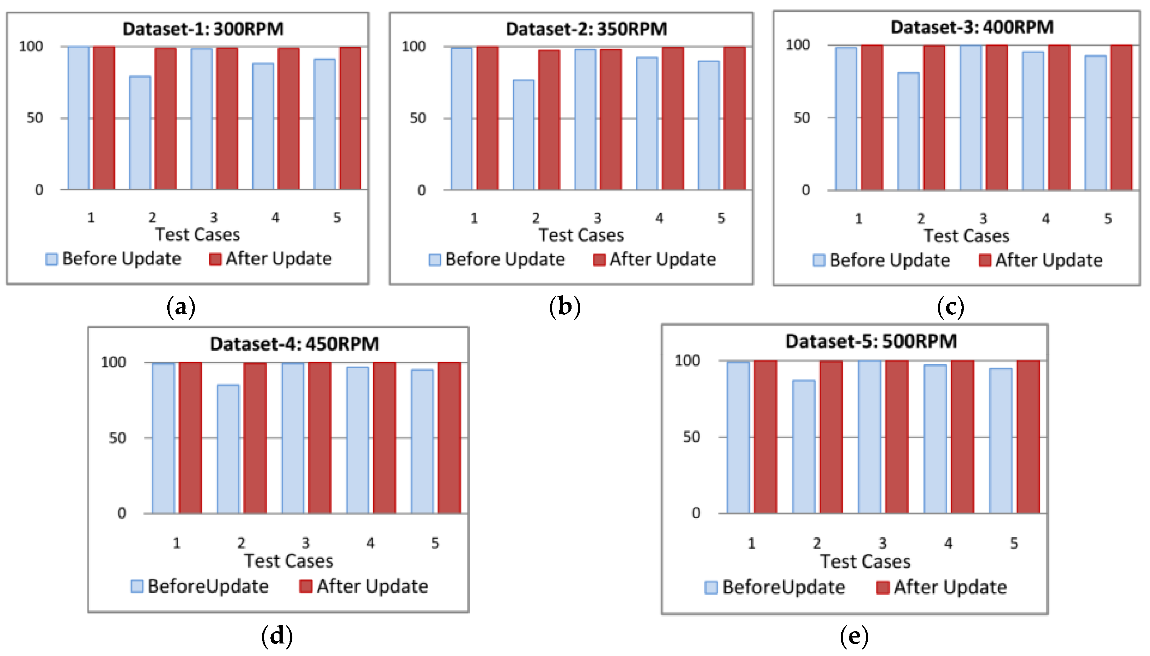
4.3. New Fault Mode Detection and System Update for Online Fault Diagnosis
4.4. Effectiveness of Online Fault Diagnosis
5. Conclusions
Author Contributions
Funding
Conflicts of Interest
References
- Zhang, P.; Du, Y.; Habetler, T.G.; Lu, B. A survey of condition monitoring and protection methods for medium-voltage induction motors. IEEE Trans. Ind. Appl. 2011, 47, 34–46. [Google Scholar] [CrossRef]
- Kang, M.; Kim, J.; Kim, J.-M.; Tan, A.C.C.; Kim, E.Y.; Choi, B.-K. Reliable Fault Diagnosis for Low-Speed Bearings Using Individually Trained Support Vector Machines with Kernel Discriminative Feature Analysis. IEEE Trans. Power Electron. 2015, 30, 2786–2797. [Google Scholar] [CrossRef]
- Xu, Y.; Zhang, K.; Ma, C.; Cui, L.; Tian, W. Adaptive Kurtogram and its applications in rolling bearing fault diagnosis. Mech. Syst. Signal Process. 2019, 130, 87–107. [Google Scholar] [CrossRef]
- Kang, M.; Islam, M.R.; Kim, J.; Kim, J.; Pecht, M. A Hybrid Feature Selection Scheme for Reducing Diagnostic Performance Deterioration Caused by Outliers in Data-Driven Diagnostics. IEEE Trans. Ind. Electron. 2016, 63, 3299–3310. [Google Scholar] [CrossRef]
- Seshadrinath, J.; Singh, B.; Panigrahi, B.K. Vibration analysis based interturn fault diagnosis in induction machines. IEEE Trans. Ind. Inform. 2014, 10, 340–350. [Google Scholar] [CrossRef]
- Zhou, W.; Lu, B.; Habetler, T.G.; Harley, R.G. Incipient Bearing Fault Detection via Motor Stator Current Noise Cancellation Using Wiener Filter. IEEE Trans. Ind. Appl. 2009, 45, 1309–1317. [Google Scholar] [CrossRef]
- Zhou, W.; Habetler, T.G.; Harley, R.G. Bearing Fault Detection via Stator Current Noise Cancellation and Statistical Control. IEEE Trans. Ind. Electron. 2008, 55, 4260–4269. [Google Scholar] [CrossRef]
- Berry, J.E. How to Track Rolling Element Bearing Health with Vibration Signature Analysis. Sound Vib. 1991, 11, 24–35. [Google Scholar]
- Jiang, F.; Zhu, Z.; Li, W.; Ren, Y.; Zhou, G.; Chang, Y. A Fusion Feature Extraction Method Using EEMD and Correlation Coefficient Analysis for Bearing Fault Diagnosis. Appl. Sci. 2018, 8, 1621. [Google Scholar] [CrossRef]
- Seshadrinath, J.; Singh, B.; Panigrahi, B.K. Investigation of vibration signatures for multiple fault diagnosis in variable frequency drives using complex wavelets. IEEE Trans. Power Electron. 2014, 29, 936–945. [Google Scholar] [CrossRef]
- Pandya, D.H.; Upadhyay, S.H.; Harsha, S.P. Fault diagnosis of rolling element bearing with intrinsic mode function of acoustic emission data using APF-KNN. Expert Syst. Appl. 2013, 40, 4137–4145. [Google Scholar] [CrossRef]
- Niknam, S.A.; Songmene, V.; Au, Y.H.J. The Use of Acoustic Emission Information to Distinguish Between Dry and Lubricated Rolling Element Bearings in Low-Speed Rotating Machines. Int. J. Adv. Manuf. Technol. 2013, 69, 2679–2689. [Google Scholar] [CrossRef]
- Eftekharnejad, B.; Carrasco, M.R.; Charnley, B.; Mba, D. The Application of Spectral Kurtosis on Acoustic Emission and Vibrations from a Defective Bearing. Mech. Syst. Signal Process. 2011, 25, 266–284. [Google Scholar] [CrossRef]
- Rauber, T.W.; Boldt, F.A.; Varejao, F.M. Heterogeneous Feature Models and Feature Selection Applied to Bearing Fault Diagnosis. IEEE Trans. Ind. Electron. 2015, 62, 637–646. [Google Scholar] [CrossRef]
- Islam, R.; Khan, S.A.; Kim, J.-M. Discriminant Feature Distribution Analysis-Based Hybrid Feature Selection for Online Bearing Fault Diagnosis in Induction Motors. J. Sens. 2016, 2016, 1–16. [Google Scholar] [CrossRef]
- Yu, K.; Lin, T.R.; Tan, J.; Ma, H. An adaptive sensitive frequency band selection method for empirical wavelet transform and its application in bearing fault diagnosis. Measurement 2019, 134, 375–384. [Google Scholar] [CrossRef]
- Yin, G.; Zhang, Y.-T.; Li, Z.-N.; Ren, G.-Q.; Fan, H.-B. Online fault diagnosis method based on Incremental Support Vector Data Description and Extreme Learning Machine with incremental output structure. Neurocomputing 2014, 128, 224–231. [Google Scholar] [CrossRef]
- Jiang, W.; Zhou, J.; Liu, H.; Shan, Y. A multi-step progressive fault diagnosis method for rolling element bearing based on energy entropy theory and hybrid ensemble auto-encoder. ISA Trans. 2019, 87, 235–250. [Google Scholar] [CrossRef] [PubMed]
- Yiakopoulos, C.T.; Gryllias, K.C.; Antoniadis, I.A. Rolling element bearing fault detection in industrial environments based on a K-means clustering approach. Expert Syst. Appl. 2011, 38, 2888–2911. [Google Scholar] [CrossRef]
- Khan, F. An initial seed selection algorithm for k-means clustering of geo referenced data to improve replicability of cluster assignments for mapping application. Appl. Soft Comput. 2012, 12, 3698–3700. [Google Scholar] [CrossRef]
- Bradley, P.S.; Fayyad, U.M. Refining initial points for K-means clustering. In Proceedings of the Fifteenth International Conference on Machine Learning, San Francisco, CA, USA, 24–27 July 1998; pp. 91–99. [Google Scholar]
- Likas, A.; Vlassis, N.; Verbeek, J.J. The global K-means clustering algorithm. Pattern Recognit. 2003, 36, 451–461. [Google Scholar] [CrossRef]
- Arthur, D.; Vassilvitskii, S. K-means ++: The Advantages of Careful Seeding. In Proceedings of the Eighteenth Annual ACM-SIAM Symposium on Discrete Algorithms, New Orleans, LA, USA, 7–9 January 2007; pp. 1027–1035. [Google Scholar]
- Kaufman, L.; Rousseeuw, P.J. Finding Groups in Data: An Introduction to Cluster Analysis; John Wiley & Sons, Inc.: Hoboken, NJ, USA, 2005. [Google Scholar]
- Tan, P.-N.; Steinbach, M.; Kumar, V. Introduction to Data Mining, 1st ed.; Pearson Addison Wessley: Boston, MA, USA, 2005. [Google Scholar]
- Rahman, M.A.; Islam, M.Z. A hybrid clustering technique combining a novel genetic algorithm with K-Means. Knowl.-Based Syst. 2014, 71, 345–365. [Google Scholar] [CrossRef]
- Kang, M.; Kim, J.; Wills, L.M.; Kim, J.-M. Time-Varying and Multi resolution Envelope Analysis and Discriminative Feature Analysis for Bearing Fault Diagnosis. IEEE Trans. Power Electron. 2015, 62, 7749–7761. [Google Scholar]
- WS Sensor, General Purpose Wideband Sensor. Available online: http://www.physicalacoustics.com/content/literature/sensors/Model_WSa.pdf (accessed on 20 May 2019).
- Bediaga, I.; Mendizabal, X.; Arnaiz, A.; Munoa, J. Ball Bearing Damage Detection Using Traditional Signal Processing Algorithms. IEEE Instrum. Meas. Mag. 2013, 16, 20–25. [Google Scholar] [CrossRef]
- Randall, R.B.; Antoni, J. Rolling Element Bearing Diagnostics—A Tutorial. Mech. Syst. Signal Process. 2011, 25, 485–520. [Google Scholar] [CrossRef]
- Li, B.; Zhang, P.-L.; Tian, H.; Mi, S.-S.; Liu, D.-S.; Ren, G.-Q. A New Feature Extraction and Selection Scheme for Hybrid Fault Diagnosis of Gearbox. Expert Syst. Appl. 2011, 38, 10000–10009. [Google Scholar] [CrossRef]
- Liu, C.; Jiang, D.; Yang, W. Global Geometric Similarity Scheme for Feature Selection in Fault Diagnosis. Expert Syst. Appl. 2014, 41, 3585–3595. [Google Scholar] [CrossRef]
- Li, Z.; Yan, X.; Tian, Z.; Yuan, C.; Peng, Z.; Li, L. Blind Vibration Component Separation and Nonlinear Feature Extraction Applied to the Non stationary Vibration Signals for the Gearbox Multi-Fault Diagnosis. Measurement 2013, 46, 259–271. [Google Scholar] [CrossRef]
- Islam, R.; Khan, S.A.; Kim, J.-M. Maximum class separability-based discriminant feature selection using a GA for reliable fault diagnosis of induction motors. Lect. Notes Artif. Intell. (LNAI) 2015, 9227, 526–537. [Google Scholar]
- Steinley, D. K-means clustering: A half-century synthesis. Br. J. Math. Stat. Psychol. 2006, 9, 1–34. [Google Scholar] [CrossRef]
- Wu, X.; Kumar, V.; Quinlan, J.R.; Ghosh, J.; Yang, Q.; Motoda, H.; McLachlan, G.J.; Ng, A.; Liu, B.; Yu, P.S.; et al. Top 10 algorithms in data mining. Knowl. Inf. Syst. 2008, 14, 1–37. [Google Scholar] [CrossRef]
- Lloyd, S.P. Least Squares Quantization in PCM. IEEE Trans. Inf. Theory 1982, 8, 129–137. [Google Scholar] [CrossRef]
- Naldi, M.C.; Campello, R.J.G.B. Comparison of distributed evolutionary k-means clustering algorithms. Neurocomputing 2015, 163, 78–93. [Google Scholar] [CrossRef]
- Zhang, Y.; Mańdziuk, J.; Quek, C.H.; Goh, B.W. Curvature-based method for determining the number of clusters. Inf. Sci. 2017, 415–416, 414–428. [Google Scholar] [CrossRef]
- Yahyaoui, H.; Own, H.S. Unsupervised clustering of service performance behaviors. Inf. Sci. 2018, 422, 558–571. [Google Scholar] [CrossRef]
- Kazmier, L.J. Schaum’s Outline of Business Statistics; McGraw Hill Professional: New York, NY, USA, 2009; p. 359. [Google Scholar]
- Yigit, H. A weighting approach for KNN classifier. In Proceedings of the 2013 International Conference on Electronics, Computer and Computation (ICECCO), Ankara, Turkey, 7–9 November 2013; pp. 228–231. [Google Scholar]


| Dataset 1 | Dataset 2 | Dataset 3 | Dataset 4 | Dataset 5 | ||
|---|---|---|---|---|---|---|
| Average RPM | 300 rpm | 350 rpm | 400 rpm | 450 rpm | 500 rpm | |
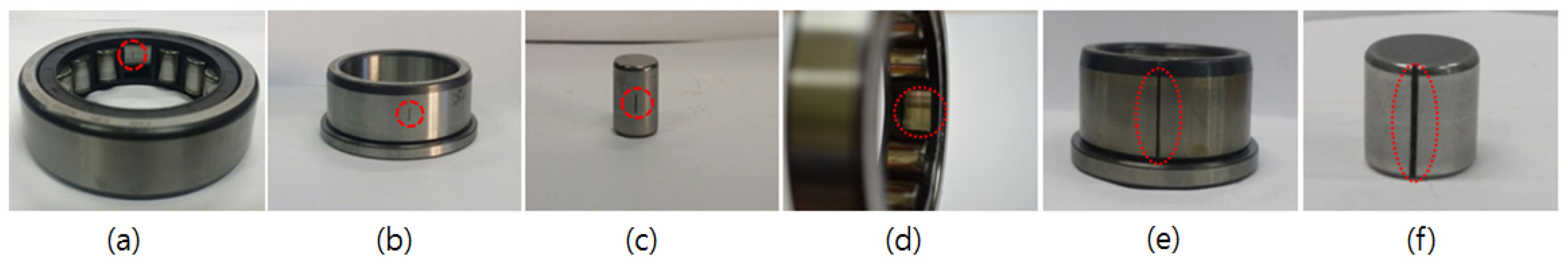
| Fault Severity | Small crack | Crack length: 3 mm, width: 0.35 mm, depth: 0.3 mm on outer raceway, inner raceway, and roller | ||||
| Big crack | Crack length: 12 mm on outer and inner raceways and 10 mm on roller, width: 0.49 mm, depth: 0.5 mm | |||||
| Initial | Test Case 1 | Update System knowledge | Test Case 2 | Update System knowledge | Test Case 3 | No Update | Test Case 4 | Update System knowledge | Test Case 5 | Update System knowledge | Final | |
| System Condition | FFB | FFB | FFB BCI 3 mm | FFB BCI 3 mm BCO 3 mm BCR 3 mm | FFB BCI 3 mm BCO 3 mm BCR 3 mm | FFB BCI 3 mm BCO 3 mm BCR 3 mm BCI 12 mm | FFB BCI 3 mm BCO 3 mm BCR 3 mm BCI 12 mm BCO 12 mm BCR 12 mm | |||||
| Unknown Signals | BCI 3 mm | BCO 3 mm BCR 3 mm | BCI 3 mm BCR 3 mm | BCI 12 mm | BCO 12 mm BCR 12 mm |
| Datasets | Test Cases | |||||||||||
|---|---|---|---|---|---|---|---|---|---|---|---|---|
| Initial | Test Case 1 | Test Case 2 | Test Case 3 | Test Case 4 | Test Case 5 | |||||||
| Features | System Knowledge | Features | System Knowledge | Features | System Knowledge | Features | System Knowledge | Features | System Knowledge | Features | System Knowledge | |
| 1 | f1~f22 | 1 × 30 × 22 | f1, f12, f13, f15 | 2 × 30 × 4 | f2, f9, f10 | 4 × 30 × 3 | f2, f9, f10 | 4 × 30 × 3 | f2, f9 | 5 × 30 × 2 | f2, f9, f13 | 7 × 30 × 3 |
| 2 | f1~f22 | 1 × 30 × 22 | f2, f9, f14 | 2 × 30 × 3 | f2, f9, f22 | 4 × 30 × 3 | f2, f9, f22 | 4 × 30 × 3 | f2, f9, f13 | 5 × 30 × 3 | f2, f9, f11, f22 | 7 × 30 × 4 |
| 3 | f1~f22 | 1 × 30 × 22 | f2, f15, f16, f20 | 2 × 30 × 4 | f2, f16 | 4 × 30 × 2 | f2, f16 | 4 × 30 × 2 | f2, f11, f15, f16 | 5 × 30 × 4 | f2, f9, f11 | 7 × 30 × 3 |
| 4 | f1~f22 | 1 × 30 × 22 | f2, f9, f13 | 2 × 30 × 3 | f2, f9, f20, f21 | 4 × 30 × 4 | f2, f9, f20, f21 | 4 × 30 × 4 | f2, f9 | 5 × 30 × 2 | f2, f9, f13 | 7 × 30 × 3 |
| 5 | f1~f22 | 1 × 30 × 22 | f2, f9 | 2 × 30 × 2 | f2, f9, f20, f21 | 4 × 30 × 4 | f2, f9, f20, f21 | 4 × 30 × 4 | f2, f9, f22 | 5 × 30 × 3 | f2, f11 | 7 × 30 × 2 |
| Datasets | Average Sensitivities Per Class with Standard Deviation | |||||||||
|---|---|---|---|---|---|---|---|---|---|---|
| Test Case | System Condition | FFB | BCI 3 mm | BCO 3 mm | BCR 3 mm | BCI 12 mm | BCO 12 mm | BCR 10 mm | Average | |
| Dataset-1: 300 RPM | Case-1 | Before Update | 100.00 (0.0) | 100.00 (0.0) | 100.00 | |||||
| Updated | 100.00 (0.0) | 100.00 (0.0) | 100.00 | |||||||
| Case-2 | Before Update | 90.45 (2.3) | 91.23 (2.1) | 65.45 (4.6) | 69.56 (4.3) | 79.17 | ||||
| Updated | 100.00 (0.0) | 94.25 (1.3) | 100.00 (0.0) | 100.00 (0.0) | 98.56 | |||||
| Case-3 | Before Update | 99.58 (0.7) | 94.36 (1.8) | 100.00 (0.0) | 100.00 (0.0) | 98.49 | ||||
| Updated | 100.00 (0.0) | 95.12 (1.1) | 100.00 (0.0) | 100.00 (0.0) | 98.78 | |||||
| Case-4 | Before Update | 93.67 (2.1) | 94.26 (1.9) | 90.23 (2.4) | 88.59 (3.9) | 73.62 (4.3) | 88.07 | |||
| Updated | 100.00 (0.0) | 93.50 (1.4) | 100.00 (0.0) | 100.00 (0.0) | 100.00 (0.0) | 98.70 | ||||
| Case-5 | Before Update | 96.56 (1.6) | 95.64 (1.7) | 91.56 (2.1) | 93.12 (1.8) | 98.26 (0.9) | 79.46 (4.1) | 82.69 (3.7) | 91.04 | |
| Updated | 100.00 (0.0) | 95.25 (1.6) | 100.00 (0.0) | 100.00 (0.0) | 100.00 (0.0) | 100.00 (0.0) | 100.00 (0.0) | 99.32 | ||
| Dataset-2: 350 RPM | Case-1 | Before Update | 100.00 (0.0) | 97.78 (1.1) | 98.89 | |||||
| Updated | 100.00 (0.0) | 100.00 (0.0) | 100.00 | |||||||
| Case-2 | Before Update | 82.23 (3.2) | 73.12 (3.9) | 75.94 (3.6) | 75.45 (3.3) | 76.69 | ||||
| Updated | 100.00 (0.0) | 89.85 (2.1) | 100.00 (0.0) | 100.00 (0.0) | 97.46 | |||||
| Case-3 | Before Update | 100.00 (0.0) | 92.35 (1.6) | 100.00 (0.0) | 99.56 (0.7) | 97.98 | ||||
| Updated | 100.00 (0.0) | 92.00 (1.5) | 100.00 (0.0) | 100.00 (0.0) | 98.00 | |||||
| Case-4 | Before Update | 93.42 (1.5) | 93.26 (1.6) | 91.86 (2.1) | 94.56 (1.3) | 89.00 (2.0) | 92.42 | |||
| Updated | 100.00 (0.0) | 97.78 (0.9) | 100.00 (0.0) | 100.00 (0.0) | 100.00 (0.0) | 99.56 | ||||
| Case-5 | Before Update | 92.65 (1.4) | 94.00 (1.0) | 92.15 (1.8) | 94.22 (1.6) | 88.25 (2.5) | 82.22 (2.8) | 86.00 (2.4) | 89.93 | |
| Updated | 100.00 (0.0) | 98.00 (0.9) | 100.00 (0.0) | 100.00 (0.0) | 100.00 (0.0) | 100.00 (0.0) | 100.00 (0.0) | 99.71 | ||
| Dataset-3: 400 RPM | Case-1 | Before Update | 96.35 (0.6) | 100.00 (0.0) | 98.18 | |||||
| Updated | 100.00 (0.0) | 100.00 (0.0) | 100.00 | |||||||
| Case-2 | Before Update | 85.00 (2.1) | 82.56 (2.8) | 77.26 (3.2) | 78.95 (2.7) | 80.94 | ||||
| Updated | 100.00 (0.0) | 98.25 (1.1) | 100.00 (0.0) | 100.00 (0.0) | 99.56 | |||||
| Case-3 | Before Update | 100.00 (0.0) | 99.56 (0.4) | 100.00 (0.0) | 99.98 (0.1) | 99.89 | ||||
| Updated | 100.00 (0.0) | 100.00 (0.0) | 100.00 (0.0) | 100.00 (0.0) | 100.00 | |||||
| Case-4 | Before Update | 97.25 (1.3) | 96.00 (1.7) | 94.56 (1.6) | 97.15 (1.0) | 92.14 (1.7) | 95.42 | |||
| Updated | 100.00 (0.0) | 100.00 (0.0) | 100.00 (0.0) | 100.00 (0.0) | 100.00 (0.0) | 100.00 | ||||
| Case-5 | Before Update | 95.45 (1.2) | 96.25 (1.1) | 96.00 (1.0) | 97.43 (0.8) | 95.64 (1.5) | 82.22 (2.8) | 86.00 (2.9) | 92.71 | |
| Updated | 100.00 (0.0) | 100.00 (0.0) | 100.00 (0.0) | 100.00 (0.0) | 100.00 (0.0) | 100.00 (0.0) | 100.00 (0.0) | 100.00 | ||
| Dataset-4: 450 RPM | Case-1 | Before Update | 99.45 (0.7) | 99.00 (0.6) | 99.23 | |||||
| Updated | 100.00 (0.0) | 100.00 (0.0) | 100.00 | |||||||
| Case-2 | Before Update | 88.00 (2.4) | 86.59 (2.3) | 82.45 (2.8) | 83.12 (2.8) | 85.04 | ||||
| Updated | 100.00 (0.0) | 98.00 (1.6) | 100.00 (0.0) | 100.00 (0.0) | 99.50 | |||||
| Case-3 | Before Update | 98.60 (1.5) | 99.45 (0.4) | 100.00 (0.0) | 99.85 (0.2) | 99.48 | ||||
| Updated | 100.00 (0.0) | 100.00 (0.0) | 100.00 (0.0) | 100.00 (0.0) | 100.00 | |||||
| Case-4 | Before Update | 97.46 (1.3) | 98.12 (1.2) | 97.23 (1.5) | 98.50 (1.3) | 93.00 (1.6) | 96.86 | |||
| Updated | 100.00 (0.0) | 100.00 (0.0) | 100.00 (0.0) | 100.00 (0.0) | 100.00 (0.0) | 100.00 | ||||
| Case-5 | Before Update | 95.89 (1.4) | 98.26 (1.1) | 96.23 (1.9) | 94.53 (2.1) | 97.58 (1.4) | 95.68 (1.6) | 88.26 (2.2) | 95.20 | |
| Updated | 100.00 (0.0) | 100.00 (0.0) | 100.00 (0.0) | 100.00 (0.0) | 100.00 (0.0) | 100.00 (0.0) | 100.00 (0.0) | 100.00 | ||
| Dataset-5: 500 RPM | Case-1 | Before Update | 97.78 (1.6) | 100.00 (0.0) | 98.89 | |||||
| Updated | 100.00 (0.0) | 100.00 (0.0) | 100.00 | |||||||
| Case-2 | Before Update | 89.00 (1.9) | 87.50 (2.1) | 85.17 (2.3) | 85.85 (2.2) | 86.88 | ||||
| Updated | 100.00 (0.0) | 98.00 (1.6) | 100.00 (0.0) | 100.00 (0.0) | 99.50 | |||||
| Case-3 | Before Update | 100.00 (0.0) | 99.98 (0.3) | 100.00 (0.0) | 100.00 (0.0) | 100.00 | ||||
| Updated | 100.00 (0.0) | 100.00 (0.0) | 100.00 (0.0) | 100.00 (0.0) | 100.00 | |||||
| Case-4 | Before Update | 97.50 (1.3) | 97.80 (1.4) | 97.43 (1.2) | 98.30 (1.2) | 94.50 (1.9) | 97.11 | |||
| Updated | 100.00 (0.0) | 100.00 (0.0) | 100.00 (0.0) | 100.00 (0.0) | 100.00 (0.0) | 100.00 | ||||
| Case-5 | Before Update | 97.12 (1.6) | 98.60 (1.4) | 95.26 (1.8) | 98.20 (1.1) | 96.80 (1.3) | 87.50 (2.6) | 90.76 (1.8) | 94.89 | |
| Updated | 100.00 (0.0) | 100.00 (0.0) | 100.00 (0.0) | 100.00 (0.0) | 100.00 (0.0) | 100.00 (0.0) | 100.00 (0.0) | 100.00 | ||
© 2019 by the authors. Licensee MDPI, Basel, Switzerland. This article is an open access article distributed under the terms and conditions of the Creative Commons Attribution (CC BY) license (http://creativecommons.org/licenses/by/4.0/).
Share and Cite
Islam, M.R.; Kim, Y.-H.; Kim, J.-Y.; Kim, J.-M. Detecting and Learning Unknown Fault States by Automatically Finding the Optimal Number of Clusters for Online Bearing Fault Diagnosis. Appl. Sci. 2019, 9, 2326. https://doi.org/10.3390/app9112326
Islam MR, Kim Y-H, Kim J-Y, Kim J-M. Detecting and Learning Unknown Fault States by Automatically Finding the Optimal Number of Clusters for Online Bearing Fault Diagnosis. Applied Sciences. 2019; 9(11):2326. https://doi.org/10.3390/app9112326
Chicago/Turabian StyleIslam, Md Rashedul, Young-Hun Kim, Jae-Young Kim, and Jong-Myon Kim. 2019. "Detecting and Learning Unknown Fault States by Automatically Finding the Optimal Number of Clusters for Online Bearing Fault Diagnosis" Applied Sciences 9, no. 11: 2326. https://doi.org/10.3390/app9112326
APA StyleIslam, M. R., Kim, Y.-H., Kim, J.-Y., & Kim, J.-M. (2019). Detecting and Learning Unknown Fault States by Automatically Finding the Optimal Number of Clusters for Online Bearing Fault Diagnosis. Applied Sciences, 9(11), 2326. https://doi.org/10.3390/app9112326