Article

Application of Multi-Dimension Input Convolutional Neural Network in Fault Diagnosis of Rolling Bearings

1
Beijing Key Laboratory of Advanced Manufacturing Technology, Beijing University of Technology, Beijing 100124, China
2
Beijing Key Laboratory of Electrical Discharge Machining Technology, Beijing 100124, China
*
Author to whom correspondence should be addressed.
Appl. Sci. 2019, 9(13), 2690; https://doi.org/10.3390/app9132690
Submission received: 28 May 2019 / Revised: 16 June 2019 / Accepted: 27 June 2019 / Published: 1 July 2019
(This article belongs to the Special Issue Fault Diagnosis of Rotating Machine)

Abstract

:

Featured Application

The proposed method in this paper is widely applied to the field of fault diagnosis of rotating machinery.

Abstract

Aiming at the problem of poor robustness of the intelligent diagnostic model, a fault diagnosis model of rolling bearing based on a multi-dimension input convolutional neural network (MDI-CNN) is proposed. Compared with the traditional convolution neural network, the proposed model has multiple input layers. Therefore, it can fuse the original signal and processed signal—making full use of advantages of the convolutional neural networks to learn the original signal characteristics automatically, and also improving recognition accuracy and anti-jamming ability. The feasibility and validity of the proposed MDI-CNN are verified, and its advantages are proved by comparison with the other related models. Moreover, the robustness of the model is tested by adding the noise to the test set. Finally, the stability of the model is verified by two experiments. The experimental results show that the proposed model improves the recognition rate, robustness and convergence performance of the traditional convolution model and has good generalization ability.

1. Introduction

Rotating machinery is the most critical component in mechanical equipment, and it is widely used in industrial production equipment [1]. Since rolling bearings are one of the most common structures in rotating machinery, the slight defects of rolling bearings may lead to the failure of the whole system and cause severe financial losses [2]. Therefore, it is of great significance to study the fault diagnosis of rolling bearings [3,4,5,6,7].
In view of bearing fault diagnosis, after a long period of exploration and research, many scholars have proposed various model-based methods [8]. Feature extraction and recognition [9] are the two most important processes in a diagnostic model. Generally, the main purpose of feature extraction is to extract the representative features, including the time domain features (kurtosis [10], crest factor [11], characteristic waveform [12], etc.), frequency domain features (Fourier transform [13], etc.), and time-frequency domain features (wavelet packet [14], empirical mode decomposition (EMD) [15,16], etc.). Then, the extracted features are entered into classification algorithms, such as support vector machines (SVM) [17] and artificial neural networks (ANN) [18].
As for the fault diagnosis of bearings, Ali et al. [19] applied the EMD to extract the time-frequency domain features, and a back propagation (BP) neural network to identify the faults. Muhammet et al. [20] proposed a novel model based on the Hilbert-Huang transform (HHT) and ANN, and obtained good performance in fault diagnosis. Xie et al. [21] suggested a bearing condition monitoring method based on EMD and SVM, which improved the accuracy of diagnosis. However, there are still some drawbacks to the fault diagnosis methods mentioned above: (1) Statistical parameters need to be extracted manually, and the professionalism of signal analysis and the importance of prior knowledge lead to poor model versatility to a large extent; (2) feature extraction process can result in loss of information; and (3) the classification model is shallow, so it is difficult to meet the requirements for diagnostic accuracy and robustness of complex mechanical systems. Therefore, an adaptive extraction and classification of features and reduction of the reliance on expert knowledge have gradually become a research hotspot in the fault diagnosis field. Many fault diagnosis models based on deep learning, which made full use of the advantages of deep network with the internal characteristics of automatic learning data, have been proposed [22,23,24,25,26]. Jia et al. [24] proposed a model based on a deep neural network (DNN), which overcame the shortcomings of the traditional diagnostic models and verified the effectiveness of DNN in the fault diagnosis field by using the data sets of rolling bearings and planetary gearboxes.
A convolutional Neural Network (CNN), as a typical deep learning method, is widely used in the field of pattern recognition. Wei et al. [27] suggested an intelligent diagnosis method for transmission line based on a CNN, which improved fault classification accuracy. Compared with other deep learning algorithms, CNNs have three advantages: Local feeling field, weight sharing, and pooling, which greatly reduce network complexity and risk of over-fitting. The input data of a CNN model can be divided into two categories, processed data and raw data. By processing of the original data, Fourier transform data [28], envelope spectrum data [29], and wavelet packet data [30,31] can be used as input data of CNN model. Although these models can achieve effective classification results, there are still some drawbacks: (1) Signal processing can result in information loss that can have an impact on diagnostic results, making an adaptive feature extraction function of CNN model not fully utilized [32,33]; and (2) the choice of a signal processing method has a great influence on diagnosis results. Therefore, the present trend is to use raw data as an input data of a CNN model. Wen et al. [34] suggested a signal-to-image conversion method that converted raw signals into two-dimensional (2D) images and then entered the obtained 2D images into the CNN model. Diagnostic performance was improved compared to other CNN methods. It is worth noting that there was no spatial relationship between the dimensions of 2D images. In [35,36,37,38], the authors developed a one-dimensional convolutional neural network (1D-CNN) model using the original signal as an input data of a CNN. These methods not only eliminated the signal processing process, but also greatly reduced model complexity. However, due to the use of the original signal as an input data, the 1D-CNN model has a great sensitivity to the noise, so it cannot be used in the case of complex and changeable noise interference in the actual production process.
In this paper, a novel intelligent fault diagnosis model, named the multi-dimension input convolutional neural network (MDI-CNN), is developed. The proposed MDI-CNN has multiple input layers so that the raw data can be entered into the model, together with the processed data to extract and identify fault features. Besides, by comparing with the other CNN models, it is proved that the proposed model has higher validity and robustness.
The main contributions of this paper can be summarized as follows.
(1) Comparing to the traditional CNN, a fusion model is proposed to achieve an effective fusion of different data types; the proposed model has multiple input layers which allows combining the benefits of each signal processing and improving the model generalization ability.
(2) The input dataset can contain both raw data and data obtained after the signal processing, which not only can improve the characteristics of the original signal, but also make full use of the advantages of the processed data in terms of clustering and anti-jamming ability; thus, the robustness and the convergence speed of the model are improved.
(3) A verification scheme is proposed to verify the validity of the proposed model, which makes the robustness and generalization performance also be validated.
This paper is organized as follows: Section 2 briefly introduces the basic theoretical basis of CNNs. Section 3 proposes the MDI-CNN model and introduces its principle. Section 4 introduces the evaluation index and the verification scheme of the proposed model. Section 5 presents the performance of the proposed model is verified by two sets of comparison experiments and analyzes and discusses the experimental results in detail. Section 6 provides our conclusions, and future work guidelines.

2. Basic Theory of the CNN

A CNN is a typical feedforward neural network, which is mainly composed of convolution layer, pooling layer, and fully connected layer. The essence is to extract the characteristics of input data by establishing multiple filters that are used to extract the topological features from the input data through the convolution and pooling operations. In recent years, the CNNs have performed well in image recognition and target detection tasks, and also have been able to deal with the fitting problems well; thus, the deep learning has been developing rapidly.
In a convolutional layer, the feature map of the previous layer is a convolution with the convolutional kernels, and the nonlinear activation function constructs the output feature map. The calculation process can be expressed as:
X j l = f i M j X i l 1 w i j l + b j l
where M j is a set of input feature map, l denotes the l t h layer, X i l 1 denotes the i t h input feature map of the l 1 t h layer, w i j l denotes the convolutional kernel which connects the i t h input feature map with j t h feature map, b denotes the bias, X j l denotes the j t h input feature map at l t h layer, f is a nonlinear activation function, and lastly, stands for the convolution operation.
The nonlinear activation function used in a neural network can be a rectified linear units (ReLU), a sigmoid function, and a hyperbolic tangent function. By considering the factors, such as gradient disappearance and calculation cost, this paper selects the ReLU activation function, which is defined as:
f x = max 0 , x
The pooling layer is used to reduce the dimension of the input feature map, which can reduce the parameters of the whole network, effectively reducing the over-fitting and the amount of calculation. The calculation process of the pooling layer is given by:
X j l = f β j l d o w n X j l 1 + b j l
where β and b are the multiplicative bias and additive bias, respectively, d o w n denotes a subsampling function, and d o w n mainly includes average pooling function, max-pooling function. After pooling operation, the number of feature maps has not changed, but the scale of feature maps shrinks a certain multiple which is determined by the pool factor size.
The fully connected layer converts the feature map into a one-dimensional feature vector that is entered into the classifier. In addition, the loss function includes mean-squared error, cross-entropy, logarithmic is significant to the CNN performance. In this paper, the cross-entropy cost function is used, which is defined as:
E = 1 m k = 1 m y k n ln l k n + 1 y k n ln 1 l k n 2
where m denotes the number of samples, l and y denote the predicted value and real value of a sample, respectively.
The network parameters are updated using the BP algorithm by calculating the gradient of the weight loss function of all the CNN layers. The objective is to minimize the loss function value by reducing the contributions of network parameters [36].

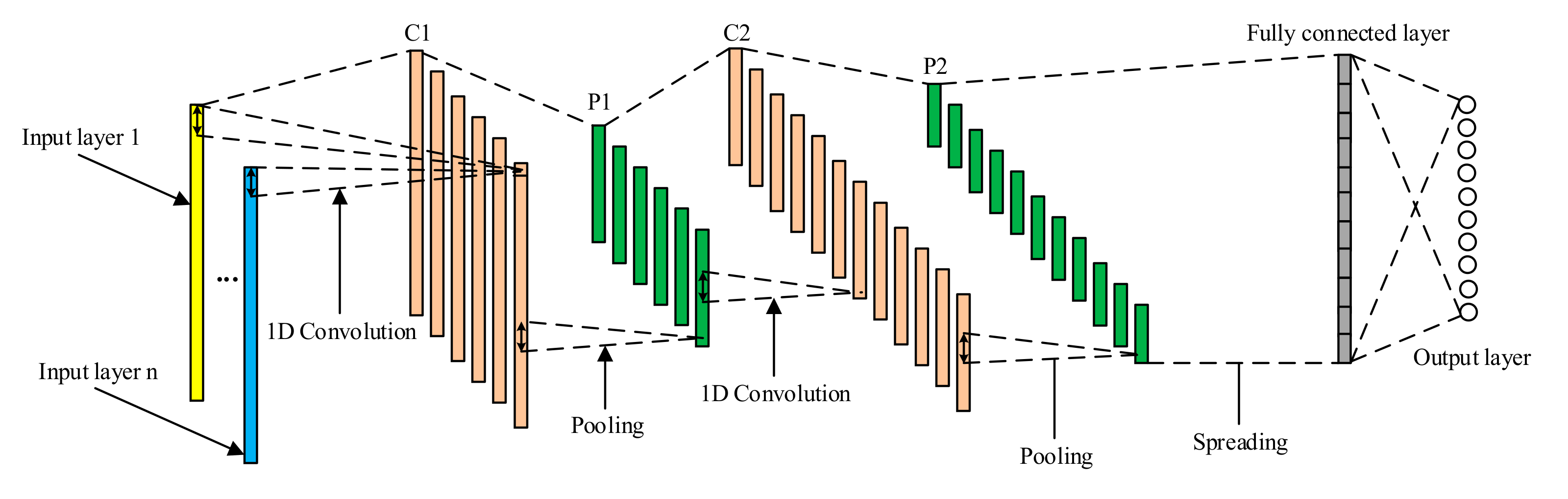
3. The Proposed Method

Due to the CNN powerful adaptive feature extraction ability for a raw signal, the combination of raw data and CNN has been employed in machinery fault diagnosis. However, the operation process of mechanical equipment is complex, and signal acquisition is often disturbed by the noise, so, the model may not perform well. Therefore, it is necessary to process a raw signal to reduce the sensitivity to the noise. It is worth considering that some information can be lost after the signal is processed; thus, the choice of signal processing algorithm is very important.
To solve the problems listed above, Guo et al. [37] proposed a multiscale convolutional neural network (MSCNN) architecture to learn the high-level robust and useful fault features at different time scales automatically directly from the complex raw vibration signals in a parallel way through the hierarchical learning. To a certain extent, the influence of high-frequency vibration and random noise on the model was reduced. However, there were some drawbacks, a raw signal was processed through low-pass filtering, the number of layers had the opposite effect on the training time and precision, and data distribution was imbalanced in the fault diagnosis field.
In order to give full play to the ability of CNN model to extract signal features, we combine the advantages of raw data and processed data and improve the anti-jamming ability, proposing a variant of the 1D-CNN called the MDI-CNN for fault diagnosis based on the intelligent fusion of multi-input layer. The structure of the developed fault diagnosis network is shown in Figure 1, wherein it can be seen that at the front end, multiple input layers are constructed to fuse different data types. The input dataset can contain both raw data and processed data, which provides rich fault features at different scales.
In the MDI-CNN network model, the ReLU function is applied as an activation function, the maximum pooling function is used to realize the reduction of a feature map, and the Softmax classifier is used to output the target category. In addition, cross entropy is used as a loss function to optimize network parameters.
Generally, the proposed model consists of three stages: A multiple data fusion stage, a feature extraction stage, and a classification stage. In the multiple data fusion stage, multiple data types are entered into the model through multiple input layers, and data fusion is performed at the first convolutional layer. In the feature extraction stage, the fused data is processed into a feature map through continuous convolutional and pooling operations, which can be regarded as signal fault characteristics. Finally, the feature maps are classified by classifier functions in the classification stage. The data fusion stage, which is an innovation point of the proposed model, is introduced in the following.

3.1. Data Fusion in MDI-CNN

Due to the impact of the environment noise, a raw signal needs to be processed before it can be entered into the traditional diagnostic model. However, diagnostic results are dependent on the selection of spectrum analysis method. In view of that, the MDI-CNN model extracts and fuses fault information of different dimensions through multiple input layers. The MDI-CNN is mainly composed of multidimensional matrix construction, initial feature extraction, and fusion model import.
In the first stage, a series of samples from different input layers are fed into the network model and then combined into a multidimensional sample matrix. After the convolution operations are performed in each dimension of the sample matrix, the multidimensional feature map matrix is fed to the next stage. Finally, the feature values at the same position in each dimension are fused through the fusion model. There are many types of data fusion methods, such as the algebraic method, principal component transformation (PCT), Bayes estimation method, and others. In this paper, the weighted fusion model based on the algebraic method is used for data fusion. The fusion model is defined as:
F = q 1 F 1 + q 2 F 2 + + q n F n
where F n denotes the n t h feature value, and q n denotes the n t h weight coefficient.
The fusion model has three advantages. First, the original signal can be processed by a variety of signal processing methods, and then all the results can be entered into the model together, which enhances model generalization ability. Second, instead of a single input layer, the MDI-CNN has multiple input layers, which not only enhances the ability to extract features, but also reduces the computation burden. Third, the model convergence speed is accelerated, due to the use of processed data that has a strong clustering compared to raw data. The general steps of the fusion model are described as follows.
Step 1: For an input layer i , L i i = 1 , 2 , , n , a multidimensional data matrix is defined as L = L 1 , L 2 , , L n , where L i denotes the i t h layer of input data, and n denotes the number of model input layers.
Step 2: Enter the i t h data matrix L i into the initial convolution layer of the CNN model. After the convolution operation, the feature map F i is obtained.
Step 3: Add a weight coefficient to each feature map. In the output position of the convolution layer, the final input of the feature map is defined as F = q 1 F 1 + q 2 F 2 + + q n F n .

3.2. General Procedure of the Propose Method

In this article, an intelligent diagnostic model called the MDI-CNN is proposed, and the entire process of the proposed method is described as below:
  • Input: Sample Set, Network parameters
  • Initialize network structure
  • While
  •   Termination condition is not valid
  •   1. Perform feature extraction and fusion in the convolutional layer
  •   2. Perform dimension reduction of a feature map in the pooling layer
  •   3. Input the feature map into the last fully connected layer, and use a Softmax activation function to obtain classification probability value
  •   4. Calculate the loss function value and update parameters using the BP algorithm
  • End while
  • Input test set into the trained model to determine model accuracy
  • Output: Predictive results for samples from test set

4. Evaluation Metrics and Validation Scheme

4.1. Evaluation Metrics

In order to evaluate the effectiveness of the proposed model, different evaluation indicators were used, including the accuracy, confusion matrix, and feature visualization. For a fault diagnosis problem of multiclass classification, the accuracy score [39,40] was used, which is a common, comprehensive metric for measuring the performance of classification methods, and it is defined as:
A c c u r a c y = T P + T N T P + T N + F P + F N
The specific meaning of TP, FP, TN, and FN is given in the following:
  • TP indicates that a true positive is correctly classified as a positive sample.
  • FP indicates that a false positive is misclassified as a positive sample.
  • TN indicates that a true negative is correctly classified as a negative sample.
  • FN indicates that a false negative is misclassified as a negative sample.
Accuracy is one of the important indexes that reflect model performance. The evaluation metrics regarding TP, FP, TN, and FN are components for creating the confusion matrix, as shown in Table 1. The feature extraction performance of the proposed model was evaluated by the visualization method of the t-distributed stochastic neighbor embedding (t-SNE).

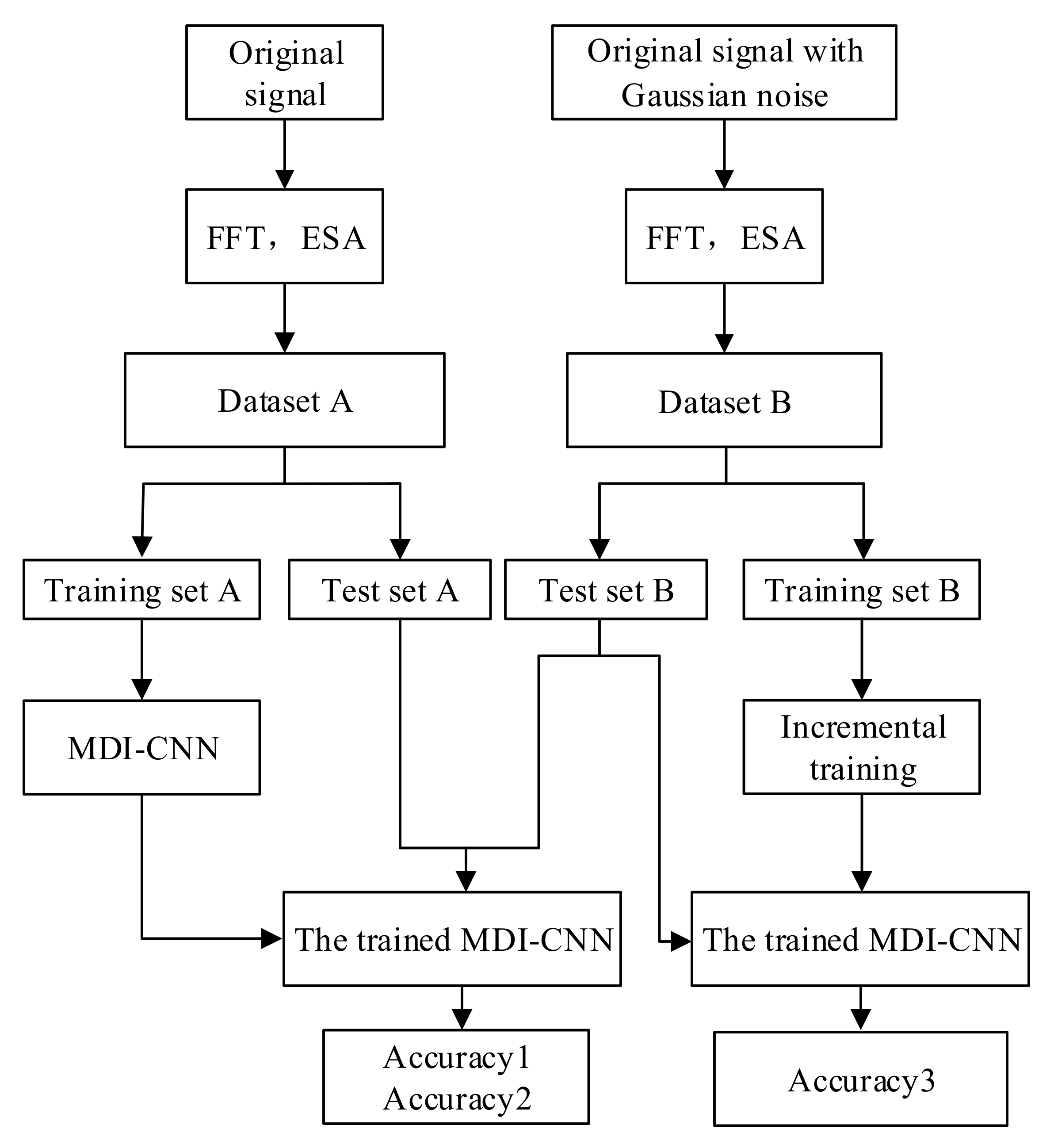
4.2. Validation Scheme

In this work, we built a CNN model with three input layers in which the raw data was used as the input data of the first layer. Spectrum data and envelope data were selected and used as input data of the second and third layers, respectively. We chose two types of rolling bearing datasets for our experiment to test the validity of the proposed MDI-CNN model. In addition, in order to verify model robustness, we employed a method that mixed the original signal with the Gaussian noise. The flowchart of the validation method is presented in Figure 2. The general process can be summarized as follows.
  • The original signal and the noisy signal that was obtained by mixing the original signal with Gaussian white noise, were processed by the fast Fourier transformation (FFT) and envelope spectrum analysis (ESA) to form the dataset A and dataset B, respectively. 87.5% of a sample in a randomly selected dataset consists of a training set, and the remaining samples are composed of a test set.
  • The network parameters, including w , b , number of iterations n u m e p o c h s , number of batch processing b a t c h s i z e , learning rate a l p h a , and weight coefficient q , were initialized.
  • The training set A was entered into the CNN model in batches for adaptive extraction of signal characteristics. The error between the predicted and actual values after the forward propagation was calculated. The error was then propagated in reverse direction by the BP algorithm in order to update the network parameters A and B layer by layer until the end of the iteration.
  • Test datasets A and B were entered into the trained MDI-CNN model to verify the validity and robustness of the model.
  • The training set B was fed into the trained MDI-CNN model for incremental training. Finally, generalization performance was validated by entering test dataset B again into the model.

5. Experimental Results and Discussion

The MDI-CNN was implemented by using MATLAB 2018a programming program, and it was run on a personal computer with a 2.6GHz CPU, inter-core i5-3230m and 8GB RAM. The computer’s system is Win10 64-bit.

5.1. Experiment 1

This section validates the effectiveness of the proposed method. In this experiment, the dataset was provided by the bearing data center of the Case Western Reserve University (CWRU). In addition, the robustness experiment was carried out by adding the noise artificially.

5.1.1. Description of Experimental Data

The CWRU dataset [41] represents a standard dataset for bearing fault diagnosis. The bearing test rig which, was used as an experimental device, mainly consisted of a 2hp motor, a power meter, a torque sensor, and an electronic control device, as shown in Figure 3. The bearing model was SKF6205, the roller diameter was 7.5 mm, the diameter of the section was 39 mm, the number of rollers was 9, and the contact angle was 0 degrees. The bearing had been machined by the Electric Discharge Machining (EDM) with three kinds of defect positions, namely rolling element damage, outer race damage, and inner race damage. The size of the damage diameter was 0.007 inches, 0.014 inches, and 0.021 inches, and three were a total of nine damage states.
In Experiment 1, the data of the bearing at the driving end was selected as the test data when the load was 1 hp, and the sampling frequency of the system was 12 kHz. In order to optimize the network training process, each signal was normalized. As shown in Figure 4, the data augment algorithm was used to carry out the overlapping sampling of samples to increase training samples, and, thus, enhance the generalization ability of the deep neural network.
Table 2 shows the composition of the test dataset, which had a total of 10 different fault types, 2000 samples for each fault type, and a total of 20,000 samples. A training set of 1750 samples was randomly selected from each fault type sample set, and the remaining 250 samples constituted the test set.
The determination of proper CNN structure and network parameters depends to a large extent on experience. According to the previous research results, the fault diagnosis model of rolling bearing based on the MDI-CNN had a three-input-layer structure, and the input data of the three layers was respectively the original signal data, the fast Fourier transform data, and the envelope spectrum analysis data. The number of network layers in the model was equal to two, and the number of neurons per layer was six and twelve, respectively. Each layer contained a convolution layer and a pooling layer. The final model parameters after many comparison tests are shown in Table 3.

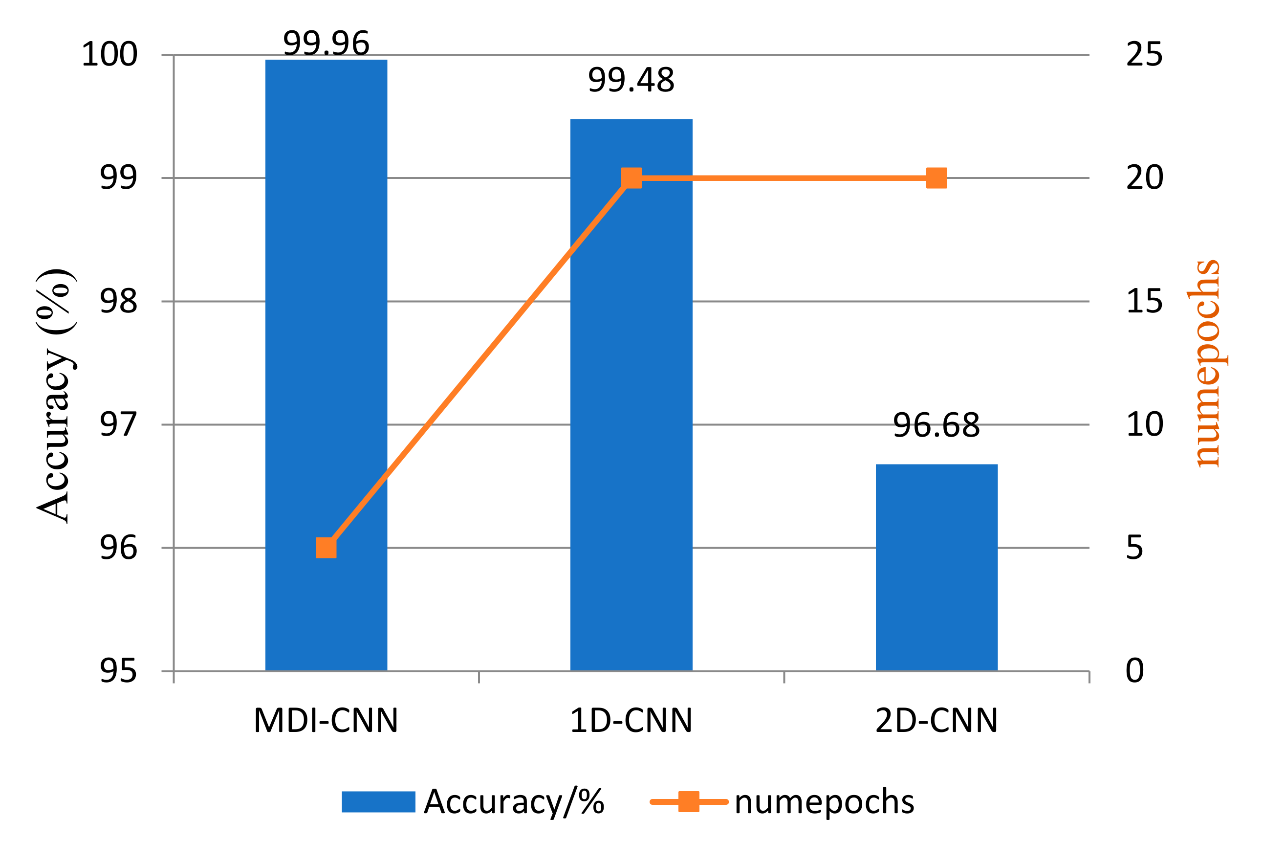
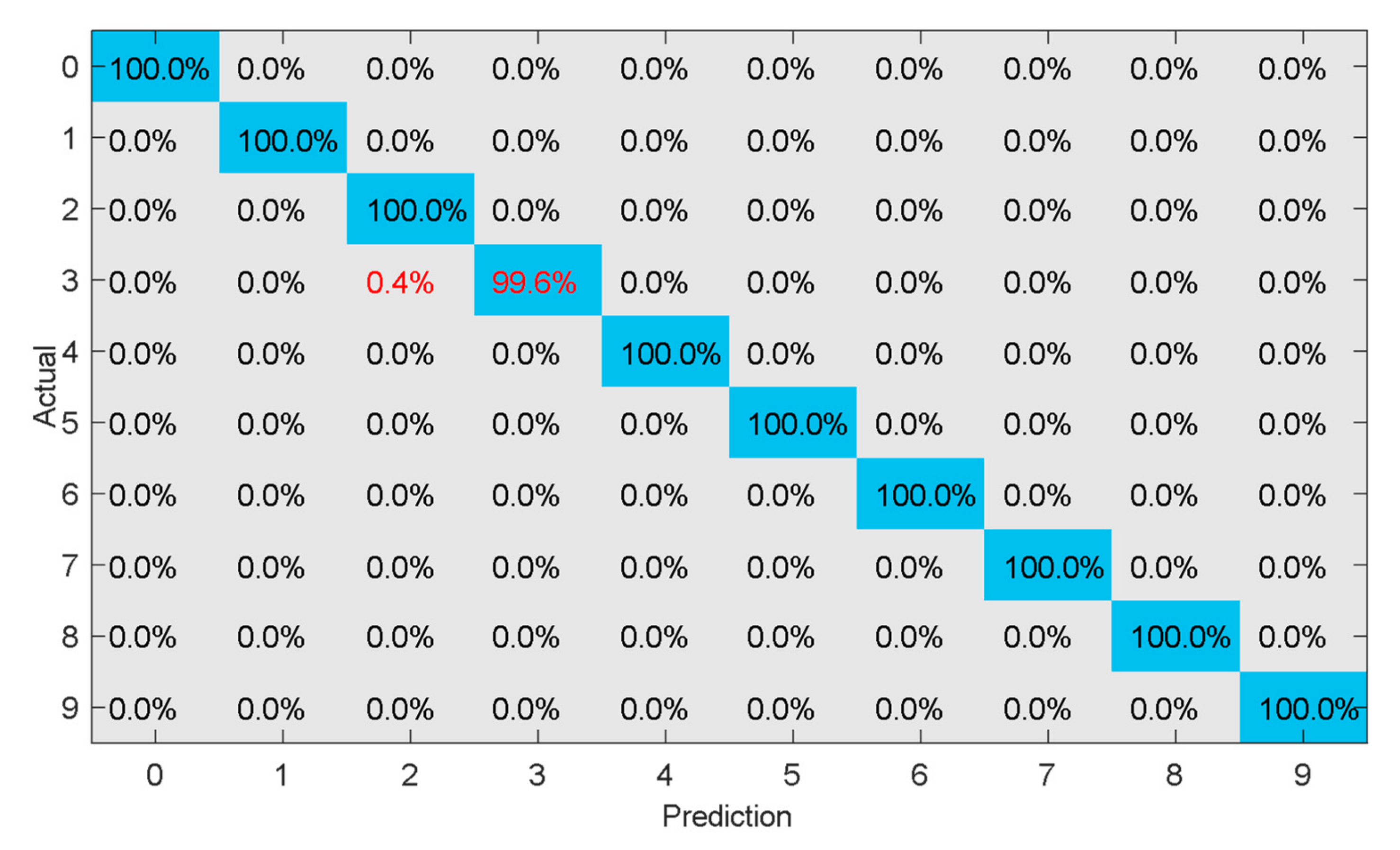
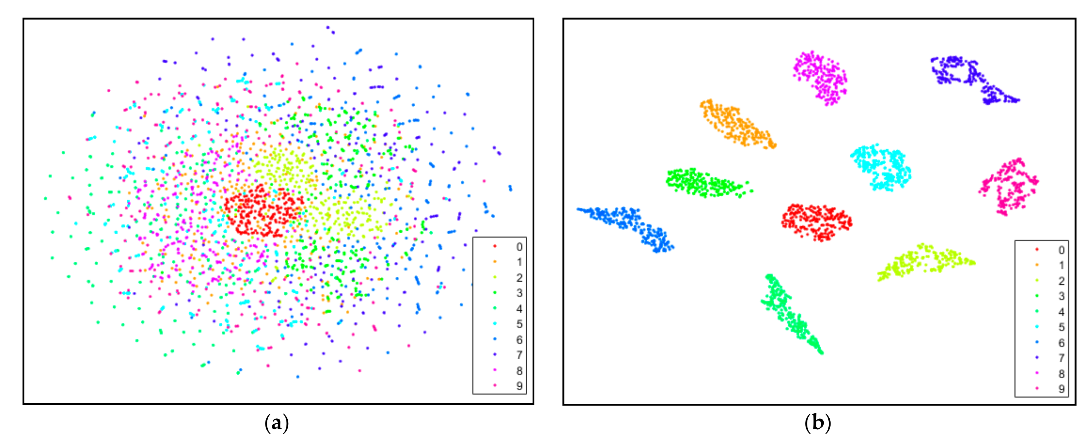
5.1.2. Performance Comparison and Discussion

The effectiveness of the MDI-CNN was validated by comparing the proposed model with other models, including the ordinary CNN (2D-CNN) model and 1D-CNN model. In the comparison process, the input data of the 1D-CNN model was an original one-dimensional signal, which was mapped to the two-dimensional matrix as the input of the ordinary CNN model. In the 2D-CNN, the number of neurons was not changed, the convolution kernel was 5 × 5, and the scale of the pool was 2 × 2. The 1D-CNN model parameters were the same as of the MDI-CNN.
The test results of the methods after twenty iterations are shown in Figure 5, where it can be seen that the training error of the MDI-CNN model was reduced to almost zero when the model reached the convergence condition after a 1000-step training, while the other two models still had the fluctuating training errors after completing 20 iterations. Thus, the MDI-CNN model improved the convergence speed of the CNN model, reducing the training time.
The accuracy of the three different models on the test set is shown in Figure 6. The results show that the fault recognition rate of the MDI-CNN model reached 99.96% after training, which proved that the proposed model was feasible and effective, and had high accuracy.
In order to present more clearly the recognition results of the MDI-CNN in each category of the test set, the confusion matrix was introduced to analyze the experimental results in detail. The results are shown in Figure 7, where the correct classification and error classification for each label are presented. In Figure 7, the horizontal coordinate represents the predicted label, and the vertical coordinate represents the actual label. Only 0.4% of samples of the label 3 in the test set was incorrectly identified as label 2, the rest of the samples were correctly classified, and eventually, the overall accuracy was 99.96%.
In order to further verify the learning ability of the MDI-CNN model for different feature categories, the dimension reduction algorithm of the t-SNE was used for feature visualization. The result of feature visualization of the raw samples and fully connected layer samples are presented in Figure 8. In Figure 8, it can be seen that the original signal was so redundant that it was difficult to distinguish between the categories. After the adaptive feature extraction of the MDI-CNN model, ten categories of samples were completely distinguished without intersecting the heterogeneous samples, which was consistent with the classification results of the proposed model.
Furthermore, the MDI-CNN model was compared with the models presented in the related literature which use the CWRU bearing database. Table 4 shows the classification accuracy of different models. The comparison results show that the recognition rate of the traditional diagnostic model varied significantly, which was because of the need to extract the fault characteristics artificially. Due to the CNN advantages in adaptive extraction of raw signal features, the classification accuracy of the CNN-based intelligent diagnostic model was generally high. In the literature [18], it can be seen that the fault characteristics of the data after spectral analysis were more prominent, so that the CNN model based on time-frequency analysis achieved a significant improvement in the recognition rate. In [31], it could be seen that the fault characteristics of the data after spectral analysis were more obvious; thus, the CNN model based on time-frequency analysis had a significant improvement in the recognition rate. The STFT-CNN model [7] achieved an accuracy rate of 99.87%. However, the two-dimensional spectral analysis data would cause some unsatisfactory results, such as the structural redundancy of the network, slow convergence speed, and long training time. In addition, an appropriate selection of a transformation method would result in the loss of information. The 1D-CNN model has been proven to be a good solution to these problems. In [23], the authors used the original signal as the input data of the 1D-CNN model, and a good classification effect was obtained, while the number of iterations was reduced. However, the original signal had a great sensitivity to the noise, which made it difficult for the 1D-CNN model to adapt to the complex and changeable noise interference in the actual production process. The model proposed in this paper represents a good combination of the advantages of the above two models, the original signal as the first layer of input data, while adding a number of spectral analysis data input layer, so in the case of short training time, it has a high recognition accuracy and robustness.
Next, the robustness of the proposed model was validated. The test set B was mixed with different SNR noise and then fed into the MDI-CNN model trained with the training set A, and the obtained classification results are shown in Figure 9. In Figure 9, it can be seen that with the increase in the noise signal strength, the recognition accuracy of all the models decreased, among which the classification accuracy of the 1D-CNN and 2D-CNN models significantly decreased when the fault signals mixed with noise were identified. The recognition rate of the proposed model was better than that of the other two models.
The incremental training was carried out by entering the training set B containing the noise into the MDI-CNN trained by the training set A to extract the fault characteristics that were not sensitive to the noise. After ten tests, the identification results of the three models are shown in Figure 10.
The comparison showed that the proposed model achieved a high recognition rate under the interference of high-intensity noise, which was better compared with the other two models. The recognition accuracy of the proposed model was further improved by the incremental training, which verified that the fault diagnosis model based on the MIL-CNN had high robustness and generalization ability.

5.2. Experiment 2

In Experiment 1, the validity and robustness of the proposed model were verified by using the open database data. In order to verify the stability of the MDI-CNN, in Experiment 2, the experimental platform for fault diagnosis of rotating machinery was selected to conduct the bearing failure experiment.

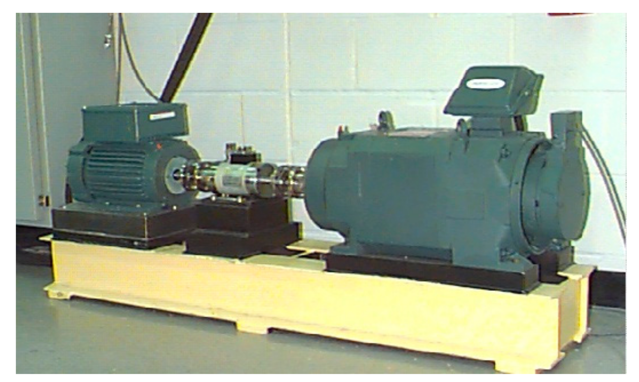
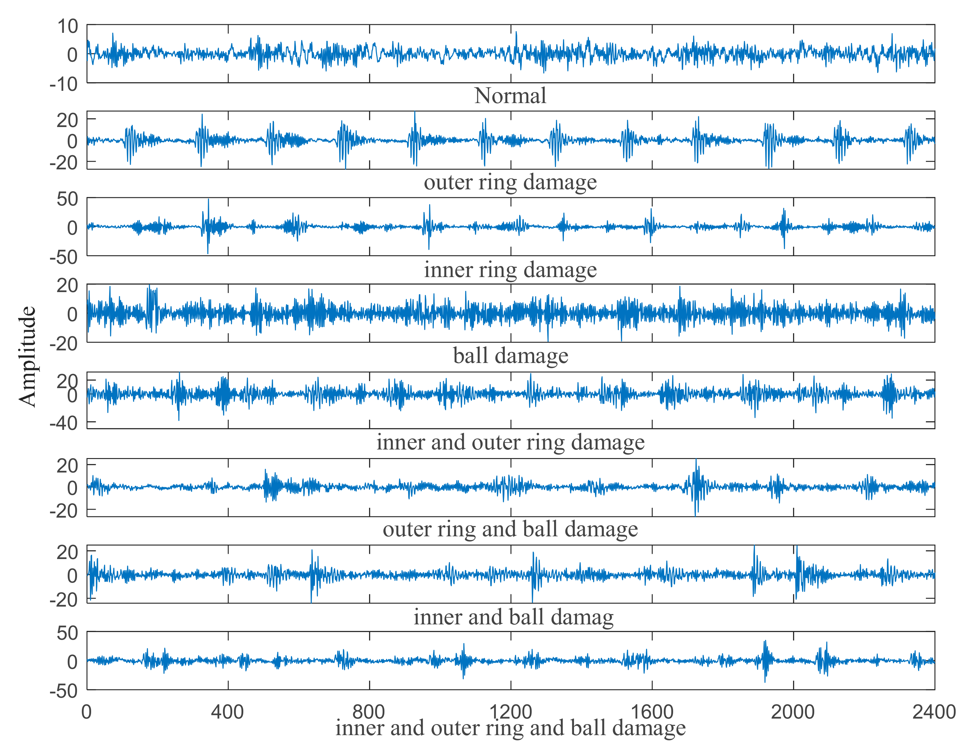
5.2.1. Description of Experimental Data

Figure 11 shows a schematic diagram of the experimental platform, where the motor is denoted as O, and A and B denote two deep groove ball bearings of type 63,701 × 3. The sampling frequency of the system was 15.3 kHz, and the measuring point was in the vertical direction of B. The bearing was artificially machined into seven faults, including outer race damage, inner race damage, rolling element damage, inner and outer race damage, outer race and rolling element damage, inner race and rolling element damage, inner and outer race and rolling element damage; the time-domain signal for all the fault types is shown in Figure 12.
The dataset was expanded by the data augment algorithm with the step length of 300. In the end, there were 2000 samples for each fault type, of which 1750 samples were randomly selected as training samples, and the rest were used as test samples. In addition, the robustness of the model was tested by adding the noise of different intensity to the original vibration signal.

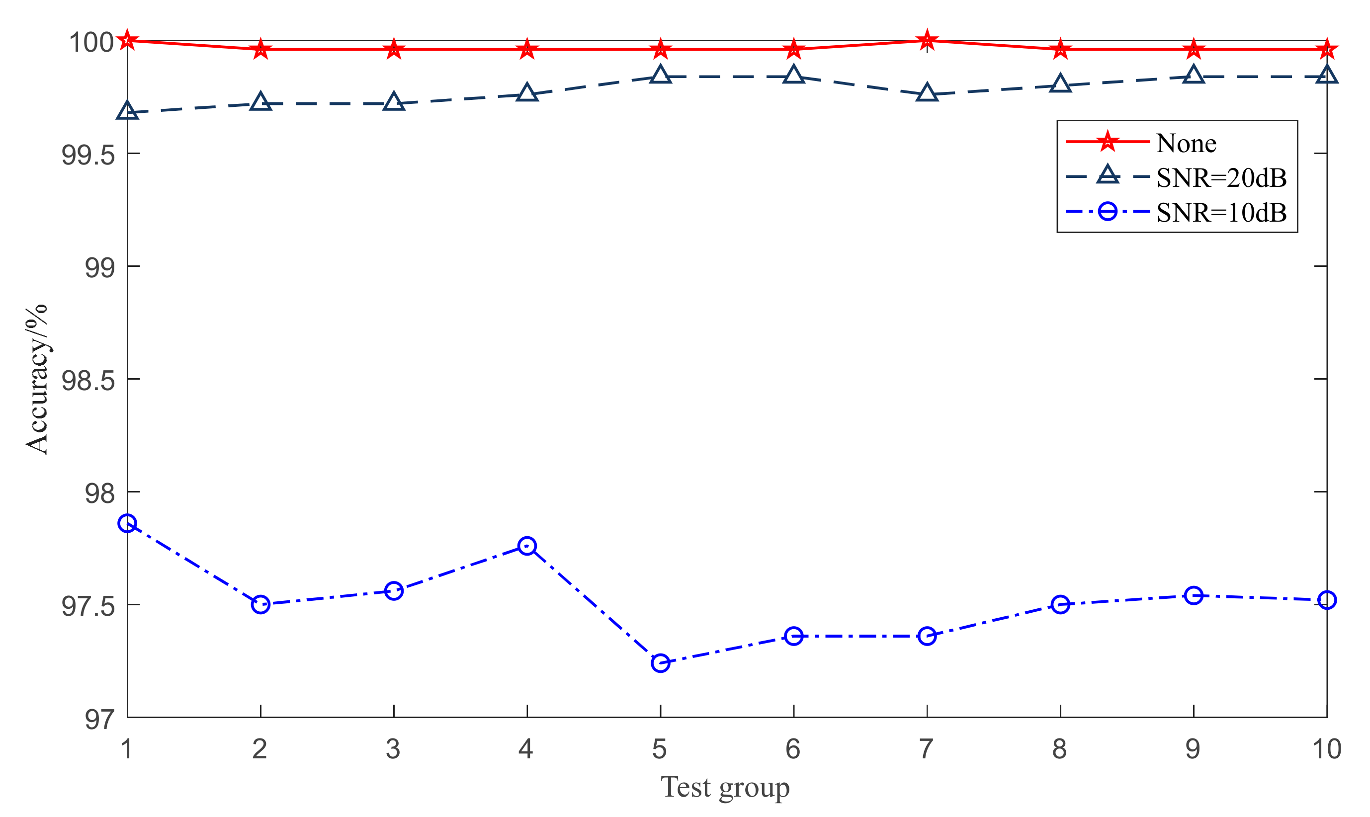
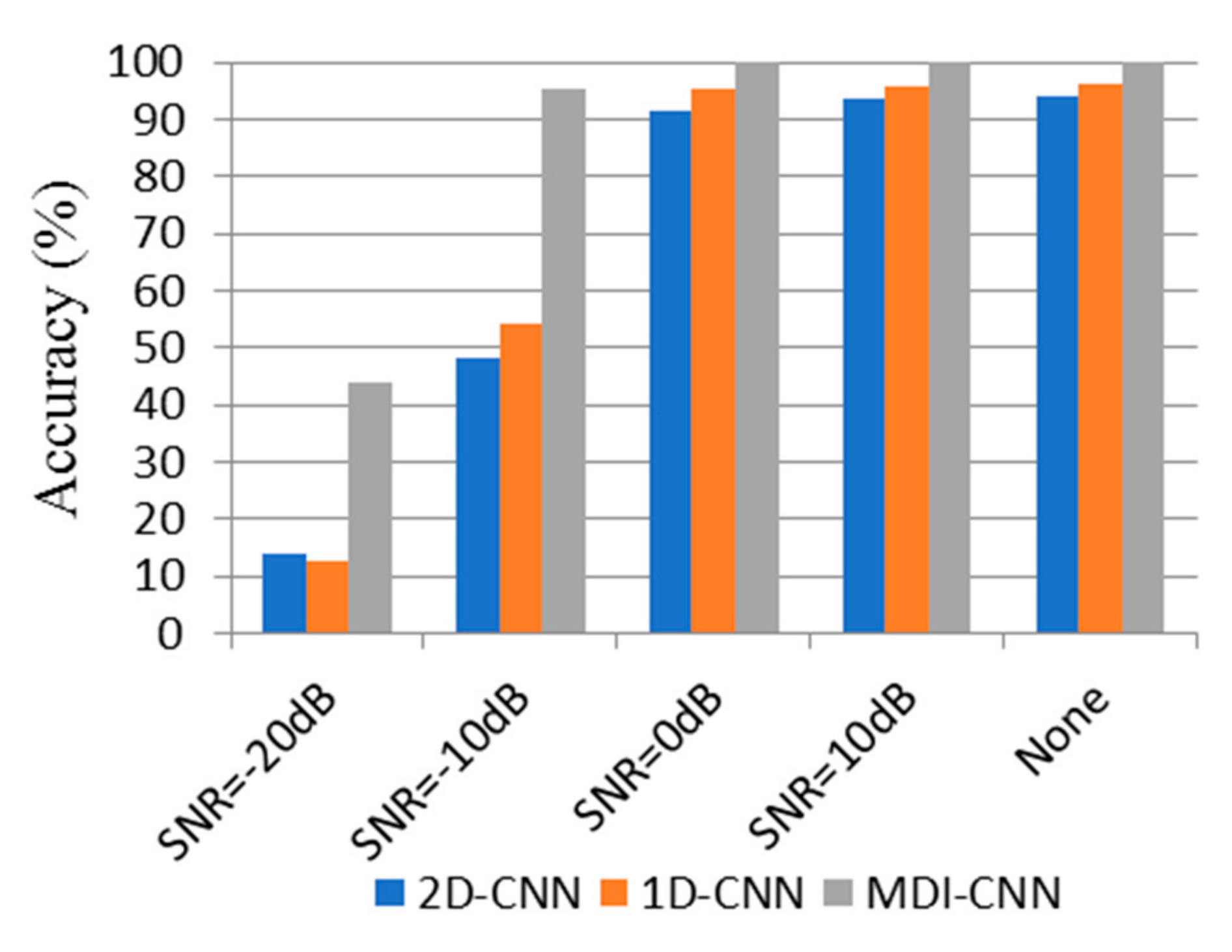
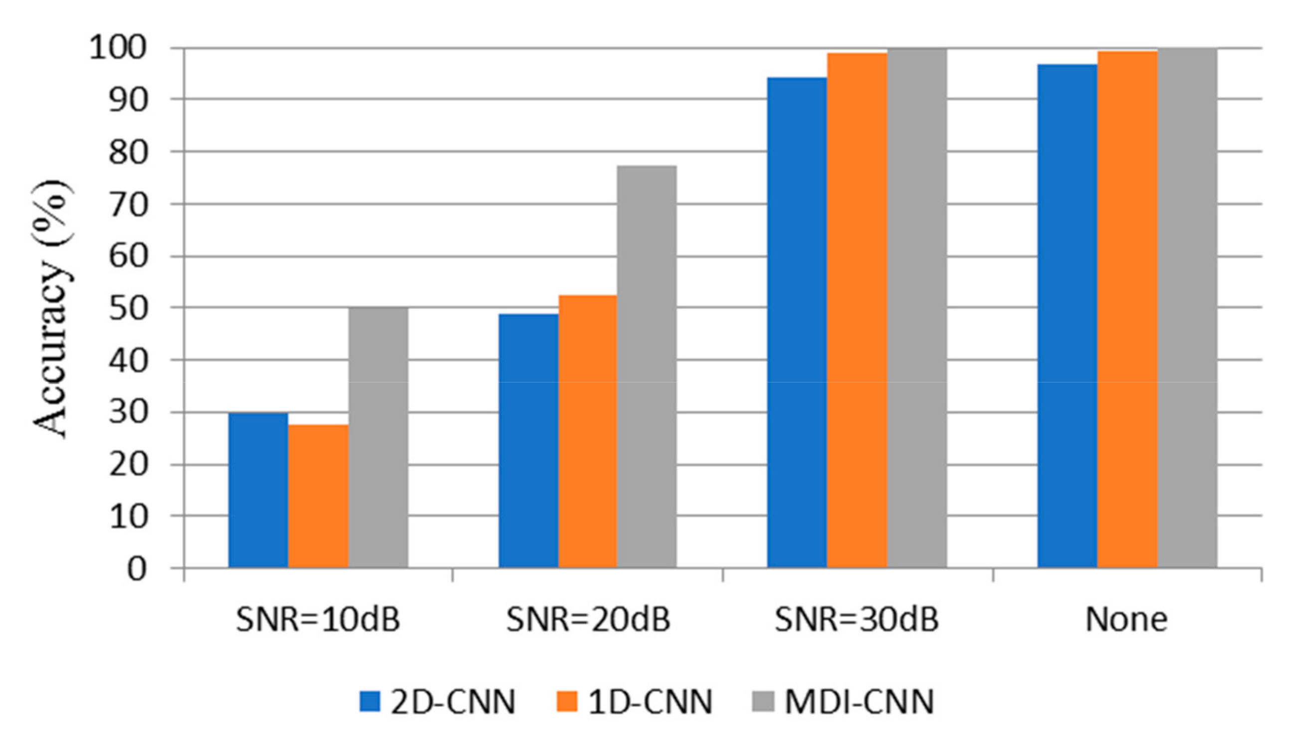
5.2.2. Performance Comparison and Discussion

Figure 13 shows the recognition accuracy for different test sets for different CNN models. In Figure 13, it can be seen that the accuracy of the three models had hardly changed under the interference of a low-intensity noise. When the noise intensity increased to −10 dB, the MDI-CNN still had a high recognition accuracy of 95.5%, but the accuracy of the other two models decreased, and it was up to about 50%. Thus, it can be concluded that the MDI-CNN model had great advantages regarding the recognition rate and robustness compared with the other two models.
In order to explain the result clearly, the feature visualization of the sample was carried out. In Figure 14, the FFT samples and ESA samples, which were obtained by signal processing of the noisy samples, are presented. Compared with the original samples, the features of the noisy samples were more confusing; thus, the recognition rate of the three models for the noisy test set was reduced. Because of the good clustering of FFT samples and ESA samples, the accuracy of the MDI-CNN model was better than of the other two models. Therefore, it can be concluded that the MDI-CNN model has good robustness because of a good inhibitory effect of spectrum analysis on noise.
In order to prove the performance advantage of the MDI-CNN model more accurately, a comparison was carried out between the proposed method and another model, using the raw data, the FFT data, and the ESA data as input data of the 2D-CNN and 1D-CNN, respectively. Table 5 shows the comparison results, where it can be seen that the proposed model had certain advantages, both regarding the recognition rate and the robustness.
Hence, the following conclusions can be drawn: (1) The accuracy and robustness of the 2D-CNN and 1D-CNN models were improved by using the FFT data and ESA data as input data; (2) compared with the ESA data, the FFT data was less sensitive to the noise; and (3) the improvement effect of the ESA data on the recognition accuracy and robustness was less obvious than of the FFT data; in other words, differently processed data had different effects on model performance.
The MDI-CNN achieves better stability and generalization performance by using multiple input layers to achieve effective fusion of multidimensional data.

6. Conclusions and Future Work

In this paper, a novel method named the MDI-CNN that fuses the multidimensional input data is proposed for fault diagnosis. The main advantage of the proposed model is the feature learning of multidimensional data by introducing a fusion model into the traditional CNN. Due to using multiple input layers, the proposed model can extract the features directly from the original vibration signal and avoid information loss. However, it can also automatically and effectively learn complementary and rich fault features of different data types directly from a signal using the multiple input layers, which greatly enhances the ability of feature extraction and fault recognition. In this paper, two experiments with rolling bearings are presented to verify the performance of the proposed model. Based on the experimental results, the following conclusions can be drawn:
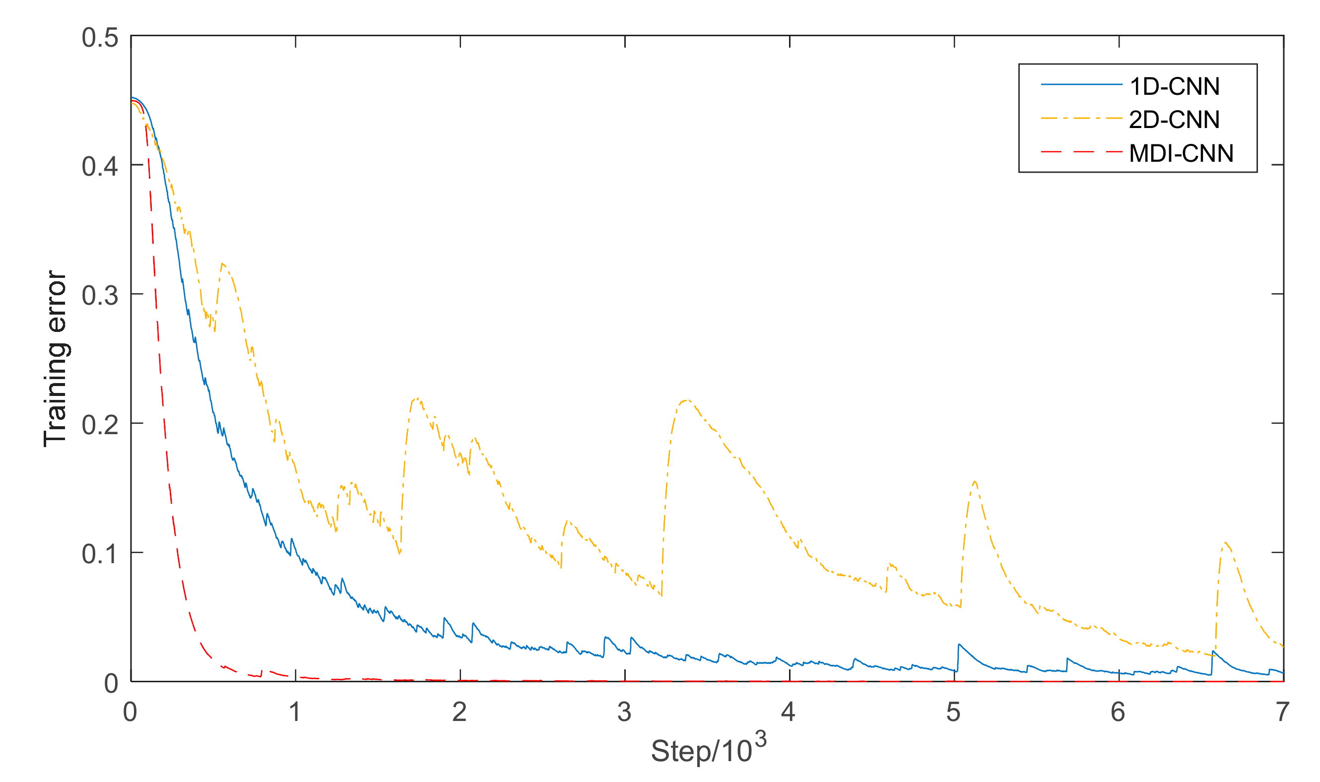
  • Compared with the traditional CNN model, the proposed model converges more quickly, has shorter training time, and achieves very good results in mixed fault identification;
  • The environmental noise seriously affects the recognition accuracy of the intelligent diagnostic model, and the proposed model can reduce the influence of noise on the recognition results. By using the noise data for incremental training, the fault recognition accuracy of the model is obviously improved;
  • Different data processing methods have different effects on diagnosis results of the traditional CNN models. The proposed model can fuse a variety of data and has high fault recognition accuracy, convergence, robustness, and generalization ability, providing a new method for real-time fault monitoring of mechanical equipment.
However, two issues need to be addressed in our future work. (1) In the experiments, the weight coefficient of the fusion model was artificially set to a constant value of one, and the other cases were not discussed. (2) The experimental data were collected in a stable environment, and then the Gaussian white noise was added artificially to the original signal to test the model sensitivity to the environmental noise. However, in the actual machining, the environmental noise is complex and changeable, which is very different from the Gaussian white noise.
Accordingly, in our future work, we will consider using an optimization algorithm to select the parameters for weight coefficients of the fusion model; also, we will collect the fault data in the actual machining environment to evaluate further the accuracy and robustness of the proposed model.

Author Contributions

Conceptualization, T.Z., H.W. and M.W.; Methodology, T.Z. and H.W.; Software, H.W. and Z.L.; Validation, T.Z., X.G. and H.W.; Formal analysis, H.W.; Investigation, Z.L.; Resources, X.G.; Writing—original draft preparation, H.W.; Writing—review and editing, H.W., M.W. and T.Z.; Visualization, Z.L.; Supervision, X.G.

Funding

This research was funded by the National Natural Science Foundation of China, grant number 51,875,008, 51,575,014 and 51,505,012, and the Beijing Municipal Education Commission Science and Technology Program project, grant number KM201,410,005,026.

Acknowledgments

This study was supported by the College of Mechanical Engineering and Applied Electronics Technology. The authors thank the Bearing Data Center of Case Western Reserve University for providing the data used in this research work, and thank Rasmus Berg Palm for providing the scripts of CNN (https://github.com/rasmusbergpalm/DeepLearnToolbox).

Conflicts of Interest

The authors declare no conflict of interest.

References

  1. El-Thalji, I.; Jantunen, E. A summary of fault modelling and predictive health monitoring of rolling element bearings. Mech. Syst. Signal Process. 2015, 60, 252–272. [Google Scholar] [CrossRef]
  2. Cui, L.L.; Wang, X.; Xu, Y.G.; Jiang, H.; Zhou, J.P. A novel Switching Unscented Kalman Filter method for remaining useful life prediction of rolling bearing. Measurement 2019, 135, 678–684. [Google Scholar] [CrossRef]
  3. Wang, H.; Ke, Y.; Luo, G.; Tang, G. Compressed sensing of roller bearing fault based on multiple down-sampling strategy. Meas. Sci. Technol. 2016, 27, 25009–25018. [Google Scholar] [CrossRef]
  4. Jiang, H.; Xia, Y.; Wang, X. Rolling bearing fault detection using an adaptive lifting multiwavelet packet with a dimension spectrum. Meas. Sci. Technol. 2013, 24, 125002–125012. [Google Scholar] [CrossRef]
  5. Chen, X.H.; Cheng, G.; Shan, X.L.; Hu, X.; Guo, Q.; Liu, X.G. Research of weak fault feature information extraction of planetary gear based on ensemble empirical mode decomposition and adaptive stochastic resonance. Measurement 2015, 73, 55–67. [Google Scholar] [CrossRef]
  6. Cui, L.L.; Huang, J.F.; Zhang, F.B.; Chu, F.L. HVSRMS localization formula and localization law: Localization diagnosis of a ball bearing outer ring fault. Mech. Syst. Signal Process. 2019, 120, 608–629. [Google Scholar] [CrossRef]
  7. Li, H.; Zhang, Q.; Qin, X.R.; Sun, Y.T. Fault diagnosis method for rolling bearings based on short-time Fourier transform and convolutional neural network. J. Vib. Shock 2018, 37, 124–131. [Google Scholar] [CrossRef]
  8. Cui, L.L.; Wang, X.; Wang, H.Q.; Wu, N. Improved Fault Size Estimation Method for Rolling Element Bearings Based on Concatenation Dictionary. IEEE Access 2019, 7, 22710–22718. [Google Scholar] [CrossRef]
  9. Cui, L.L.; Li, B.B.; Ma, J.F.; Jin, Z. Quantitative trend fault diagnosis of a rolling bearing based on Sparsogram and Lempel-Ziv. Measurement 2018, 128, 410–418. [Google Scholar] [CrossRef]
  10. Tian, J.; Morillo, C.; Azarian, M.H.; Pecht, M. Motor bearing fault detection using spectral kurtosis-based feature extraction coupled with K-nearest neighbor distance analysis. IEEE Ind. Electron. Soc. 2016, 63, 1793–1803. [Google Scholar] [CrossRef]
  11. Bhadane, M.; Ramachandran, K.I. Bearing fault identification and classification with convolutional neural network. In Proceedings of the 2017 International Conference on Circuit, Kollam, India, 20–21 April 2017; pp. 1–5. [Google Scholar] [CrossRef]
  12. Cui, L.L.; Yao, T.C.; Zhang, Y. Application of pattern recognition in gear faults based on the matching pursuit of a characteristic waveform. Measurement 2017, 104, 212–222. [Google Scholar] [CrossRef]
  13. Zhang, Z.; Verma, A.; Kusiak, A. Fault analysis and condition monitoring of the wind turbine gearbox. IEEE Trans. Energy Convers. 2012, 27, 526–535. [Google Scholar] [CrossRef]
  14. Zhang, Z.; Wang, Y.; Wang, K. Fault diagnosis and prognosis using wavelet packet decomposition, Fourier transform and artificial neural network. J. Intell. Manuf. 2013, 24, 1213–1227. [Google Scholar] [CrossRef]
  15. Lei, Y.; Zuo, M.J. Fault diagnosis of rotating machinery using an improved HHT based on EEMD and sensitive IMFs. Meas. Sci. Technol. 2009, 20, 125701–125713. [Google Scholar] [CrossRef]
  16. Lei, Y.; Lin, J.; He, Z.; Zuo, M.J. A review on empirical mode decomposition in fault diagnosis of rotating machinery. Mech. Syst. Signal Process. 2013, 35, 108–126. [Google Scholar] [CrossRef]
  17. Liu, J.; Li, Y.F.; Zio, E. A SVM framework for fault detection of the braking system in a high-speed train. Mech. Syst. Signal Process. 2017, 87, 401–409. [Google Scholar] [CrossRef]
  18. Yang, Y.; Yu, D.; Cheng, J. A roller hearing fault diagnosis method baesd on EMD energy entropy and ANN. J. Sound Vib. 2006, 294, 269–277. [Google Scholar] [CrossRef]
  19. Ali, J.B.; Fnaiech, N.; Saidi, L.; Chebel-Morello, B.; Fnaiech, F. Application of empirical mode decomposition and artificial neural network for automatic bearing fault diagnosis based on vibration signals. Appl. Acoust. 2015, 89, 16–27. [Google Scholar] [CrossRef]
  20. Unal, M.; Onat, M.; Demetgul, M.; Kucuk, H. Fault diagnosis of rolling bearings using a genetic algorithm optimized neural network. Measurement 2014, 58, 187–196. [Google Scholar] [CrossRef]
  21. Xie, N.; Ma, F.; Zheng, B. Rolling element bearing diagnostic based on EEMD and SVM. In Proceedings of the 12th World Congress on Intelligent Control and Automation (WCICA), Guilin, China, 12–15 June 2016; pp. 1658–1662. [Google Scholar] [CrossRef]
  22. Ding, X.; He, Q. Energy-Fluctuated Multiscale Feature Learning with Deep ConvNet for Intelligent Spindle Bearing Fault Diagnosis. IEEE Trans. Instrum. Meas. 2017, 66, 1926–1935. [Google Scholar] [CrossRef]
  23. Shao, H.; Jiang, H.; Zhao, H.; Wang, F. A novel deep autoencoder feature learning method for rotating machinery fault diagnosis. Mech. Syst. Signal Process. 2017, 95, 187–204. [Google Scholar] [CrossRef]
  24. Jia, F.; Lei, Y.; Lin, J.; Zhou, X.; Lu, N. Deep neural networks: A promising tool for fault characteristic mining and intelligent diagnosis of rotating machinery with massive data. Mech. Syst. Signal Process. 2016, 72, 303–315. [Google Scholar] [CrossRef]
  25. Tamilselvan, P.; Wang, P. Failure diagnosis using deep belief learning based health state classification. Reliab. Eng. Syst. Saf. 2013, 115, 124–135. [Google Scholar] [CrossRef]
  26. Gan, M.; Wang, C.; Zhu, C. Construction of hierarchical diagnosis network based on deep learning and its application in the fault pattern recognition of rolling element bearings. Mech. Syst. Signal Process. 2015, 72 –73, 92–104. [Google Scholar] [CrossRef]
  27. Dong, W.; Qingwu, G.; Wenqing, L. Research on internal and external fault diagnosis and fault-selection of transmission line based on convolutional neural network. Proc. CSEE 2016, 36, 21–28. [Google Scholar] [CrossRef]
  28. Zhang, W.; Zhang, F.; Chen, W.; Jiang, Y.; Song, D. Fault State Recognition of Rolling Bearing Based Fully Convolutional Network. Comput. Sci. Eng. 2018, 1. [Google Scholar] [CrossRef]
  29. Appana, D.K.; Alexander, P.; Jong-Myon, K. Reliable fault diagnosis of bearings with varying rotational speeds using envelope spectrum and convolution neural networks. Soft Comput. 2018, 22, 6719–6729. [Google Scholar] [CrossRef]
  30. Guo, S.; Yang, T.; Gao, W.; Zhang, C. A Novel Fault Diagnosis Method for Rotating Machinery Based on a Convolutional Neural Network. Sensors 2018, 18, 1429. [Google Scholar] [CrossRef] [PubMed]
  31. Han, Y.; Tang, B.P.; Deng, L. Multi-level wavelet packet fusion in dynamic ensemble convolutional neural network for fault diagnosis. Measurement 2018, 127, 246–255. [Google Scholar] [CrossRef]
  32. Lu, C.; Zhou, B.; Wang, Z.Y. Intelligent fault diagnosis of rolling bearing using hierarchical convolutional network based health state classification. Adv. Eng. Inform. 2017, 32, 139–151. [Google Scholar] [CrossRef]
  33. Fuan, W.; Hongkai, J.; Haidong, S.; Wenjing, D.; Shuaipeng, W. An adaptive deep convolutional neural network for rolling bearing fault diagnosis. Meas. Sci. Technol. 2017, 28, 95005–95022. [Google Scholar] [CrossRef]
  34. Wen, L.; Li, X.; Gao, L.; Zhang, Y. A New Convolutional Neural Network-Based Data-Driven Fault Diagnosis Method. IEEE Trans. Ind. Electron. 2018, 65, 5990–5998. [Google Scholar] [CrossRef]
  35. Peng, D.; Liu, Z.; Wang, H.; Qin, Y.; Jia, L. A Novel Deeper One-Dimensional CNN With Residual Learning for Fault Diagnosis of Wheelset Bearings in High-Speed Trains. IEEE Access 2019, 7, 10278–10293. [Google Scholar] [CrossRef]
  36. Zhang, W.; Peng, G.; Li, C.; Chen, Y.; Zhang, Z. A New Deep Learning Model for Fault Diagnosis with Good Anti-Noise and Domain Adaptation Ability on Raw Vibration Signals. Sensors 2017, 17, 425. [Google Scholar] [CrossRef] [PubMed]
  37. Levent, E.; Turker, I.; Serkan, K. A Generic Intelligent Bearing Fault Diagnosis System Using Compact Adaptive 1D CNN Classifier. J. Signal Process. Syst. 2018, 91, 179–189. [Google Scholar] [CrossRef]
  38. Zan, T.; Liu, Z.; Wang, H.; Wang, M.; Gao, X. Control chart pattern recognition using the convolutional neural network. J. Intell. Manuf. 2019, 30. [Google Scholar] [CrossRef]
  39. Jiang, G.; He, H.; Yan, J.; Xie, P. Multiscale Convolutional Neural Networks for Fault Diagnosis of Wind Turbine Gearbox. IEEE Trans. Ind. Electron. 2019, 66, 3196–3207. [Google Scholar] [CrossRef]
  40. He, H.B.; Garcia, E.A. Learning from imbalanced data. IEEE Trans. Knowl. Data Eng. 2009, 21, 1263–1284. [Google Scholar] [CrossRef]
  41. Li, X.; Zhang, W.; Ding, Q. A robust intelligent fault diagnosis method for rolling element bearings based on deep distance metric learning. Neurocomputing 2018, 310, 77–95. [Google Scholar] [CrossRef]
  42. Qu, J.L.; Yu, L.; Yuan, T.; Tian, Y.; Gao, F. Adaptive fault diagnosis algorithm for rolling bearings based on one-dimensional convolutional neural network. Chin. J. Sci. Instrum. 2018, 39, 134–143. [Google Scholar] [CrossRef]
Figure 1. The structure of the Multi-Dimension Input convolutional neural network. C1 and C2 represent the convolutional layer 1 and convolutional layer 2, respectively, and P1 and P2 represent the pooling layer 1 and pooling layer 2, respectively.
Applsci 09 02690 g001
Figure 2. The flowchart of the validation method for the MDI-CNN model. Accuracy 1 and Accuracy 2 represent the classification accuracy obtained by entering normal test samples and test sample containing the noise into the trained MDI-CNN, respectively, and Accuracy 3 indicates the classification accuracy of the model after the incremental training on the noisy test samples. MDI-CNN, Multi-Dimension Input convolutional neural network; FFT, Fourier transformation; ESA, envelope spectrum analysis.
Applsci 09 02690 g002
Figure 3. Image of the bearing test rig.
Applsci 09 02690 g003
Figure 4. The method of data augment.
Applsci 09 02690 g004
Figure 5. The training errors.
Applsci 09 02690 g005
Figure 6. The accuracy of different models.
Applsci 09 02690 g006
Figure 7. Confusion matrix results with MDI-CNN.
Applsci 09 02690 g007
Figure 8. Feature visualization of different samples. (a) The raw samples. (b) Fully connected layer sample.
Applsci 09 02690 g008
Figure 9. Testing diagnosis results of different models under different noise intensity.
Applsci 09 02690 g009
Figure 10. Testing the accuracy of MDI-CNN after incremental training.
Applsci 09 02690 g010
Figure 11. Schematic diagram of the experimental platform.
Applsci 09 02690 g011
Figure 12. The time-domain signal for different fault types.
Applsci 09 02690 g012
Figure 13. Testing diagnosis results of different models under different noise intensity.
Applsci 09 02690 g013
Figure 14. Feature visualization of different samples. (a) Feature visualization of raw samples; (b) Feature visualization of noisy samples; (c) Feature visualization of FFT samples; (d) Feature visualization of ESA samples.
Applsci 09 02690 g014
Table 1. The model of the confusion matrix.
Actual ValuePredicted Value
Label 1Label 2
Label 1TPFP
Label 2FNTN
Table 2. The experimental data.
Damage PositionNoneScroll BodyInner RingOuter Ring
Label0123456789
Damage diameter/inch00.0070.0140.0210.0070.0140.0210.0070.0140.021
Training set1750175017501750175017501750175017501750
Test set250250250250250250250250250250
Table 3. The MDI-CNN parameters; numepochs denotes the number of iterations of the model, batchsize denotes the number of samples processed per batch by the model during the batch training, and alpha denotes the learning rate.
Parameter NameC1 LayerP1 LayerC2 LayerP2 LayerSpacing
Parameter value 25 × 1 8 × 1 20 × 1 4 × 1 59
Parameter namenumepochsbatchsizealphaq1, q2, q3Number of neurons
Parameter value5500.05(1, 1, 1)(6, 12)
Table 4. Classification accuracy of different models.
Algorithm ModelNumber of EpochsAccuracy (%)
FFT-SVM-84.20
Wavelet-ANN-88.54
EMD-ANN-96.24
DWT-CNN [39]6099.80
PSO-CNN [31] 2092.84
WP-PSO-CNN [31]2099.71
STFT-CNN [7]1699.87
ACNN-FD [42]1299.40
MDI-CNN599.96
Table 5. Diagnosis results of different models.
ModelTraining SetNumber of EpochsSNR of Noise in Test SetAccuracy (%)
2D-CNNTwo-dimensional raw data20None93.85
−10 dB48.35
Two-dimensional FFT data10None99.00
−10 dB75.40
Two-dimensional ESA data10None97.50
−10 dB59.85
1D-CNNOne-dimensional raw data20None96.15
−10 dB54.35
One-dimensional FFT data10None99.85
−10 dB94.10
One-dimensional ESA data10None96.50
−10 dB57.55
MDI-CNNRaw data, FFT data, ESA data5None99.95
−10 dB95.50

