Ground Subsidence Investigation in Fuoshan, China, Based on SBAS-InSAR Technology with TerraSAR-X Images

Abstract
1. Introduction
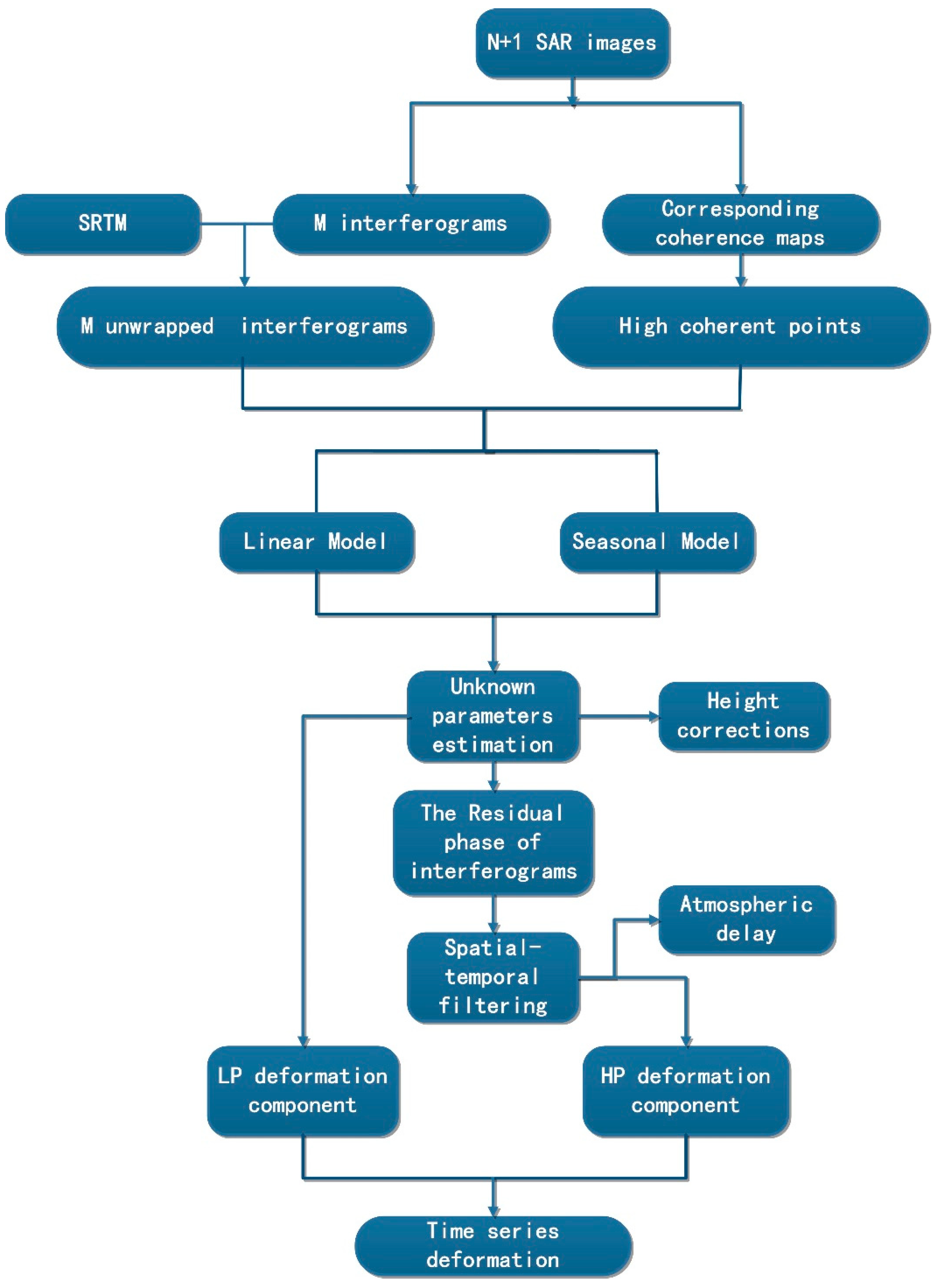
2. Methodology
2.1. SBAS-InSAR Technology Based on the Linear Model
2.2. Seasonal Model
3. Experiment
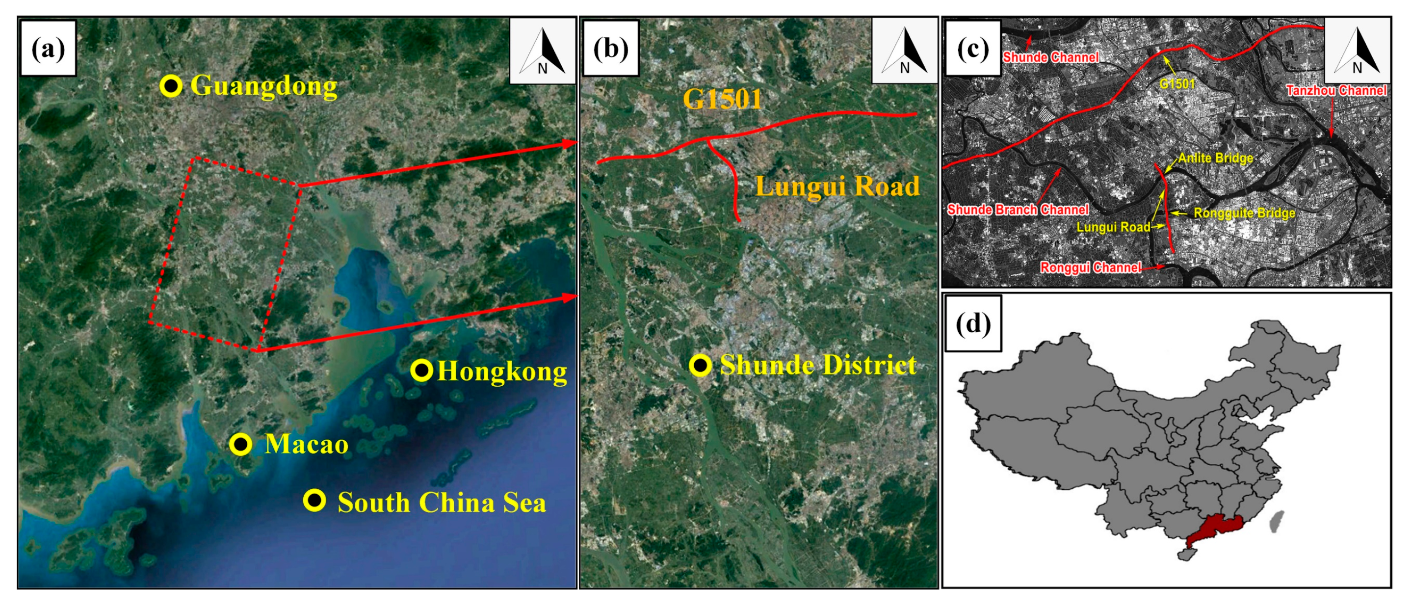
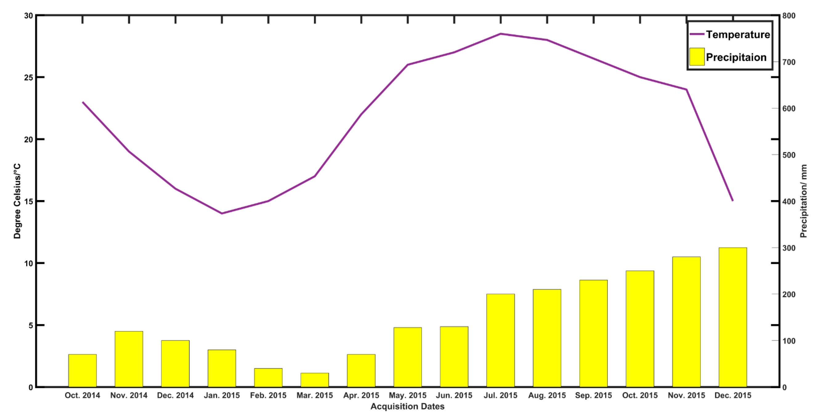
3.1. Study Area
3.2. SAR Acquisitions and Data Processing
4. Results and Discussion
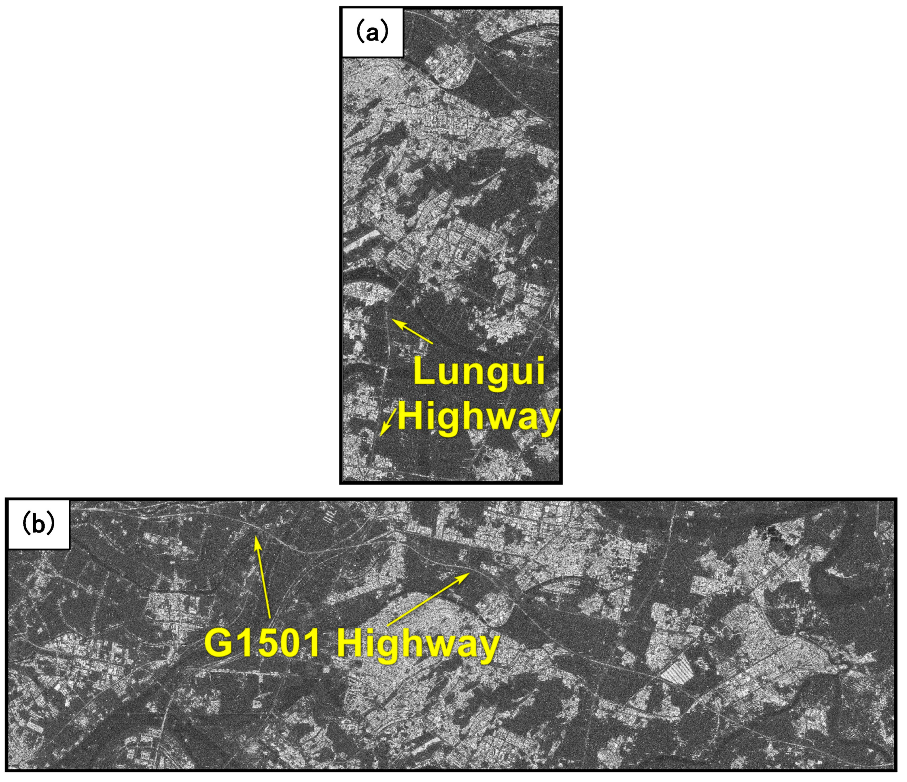
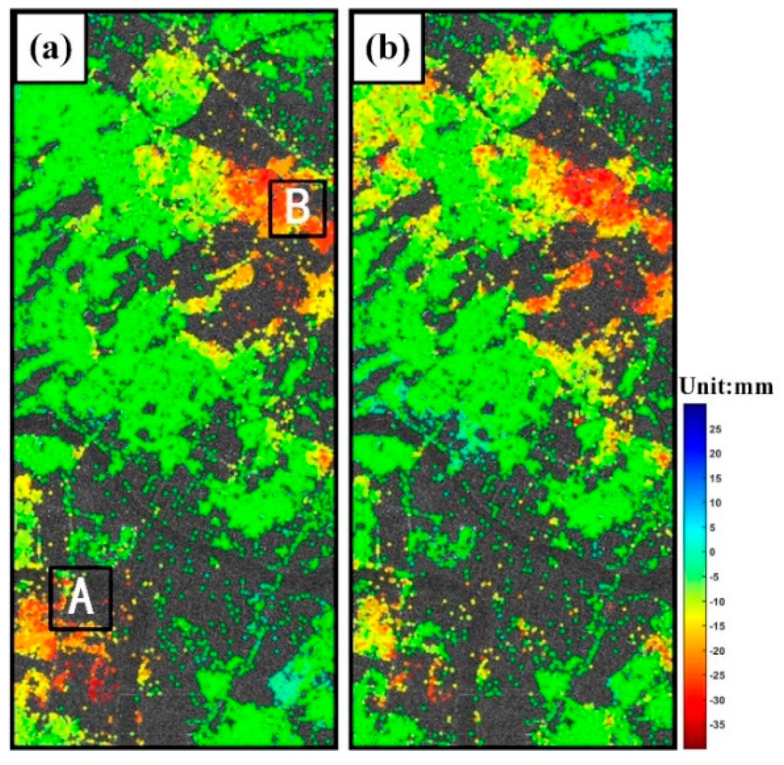
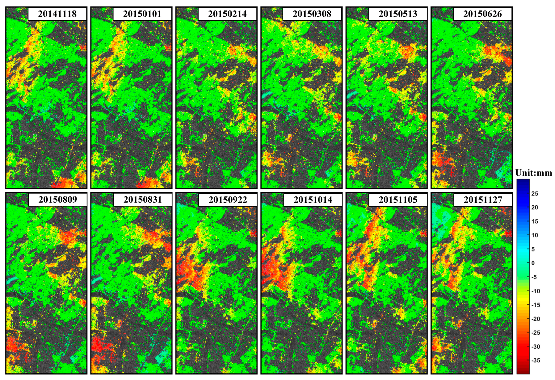
4.1. Lungui Highway
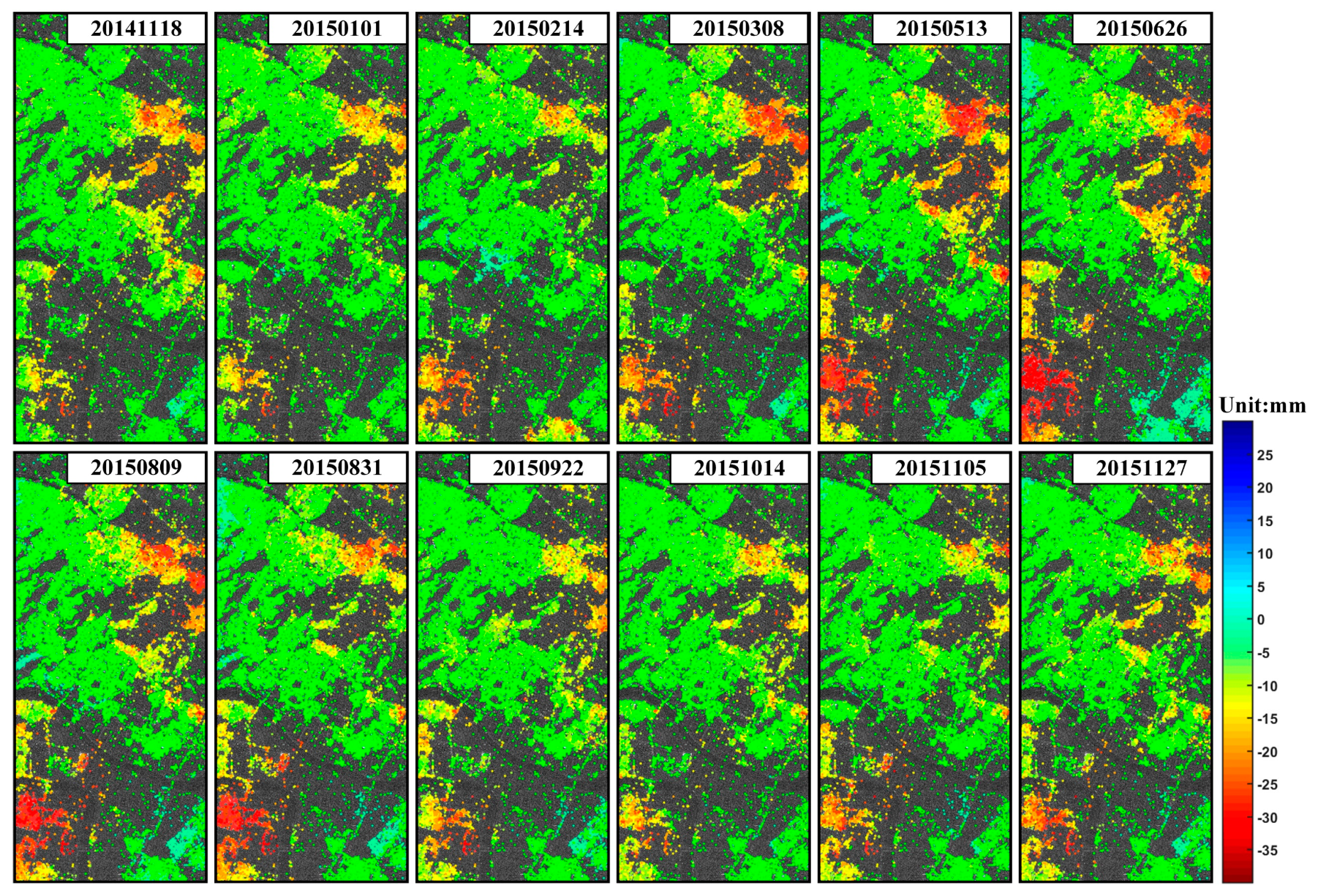
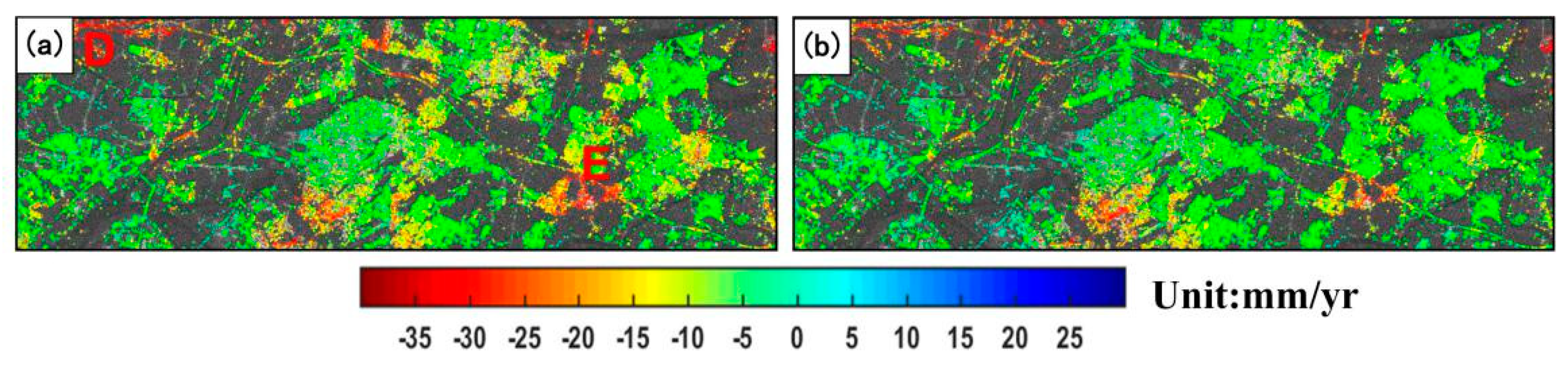
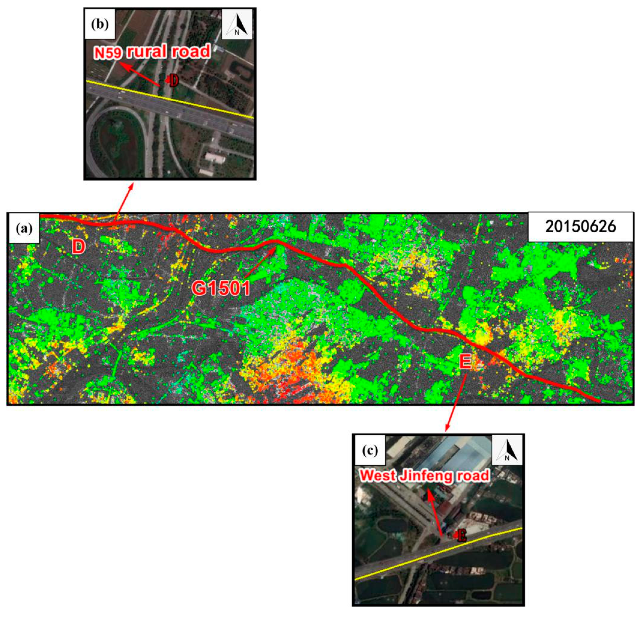
4.2. G1501 Highway
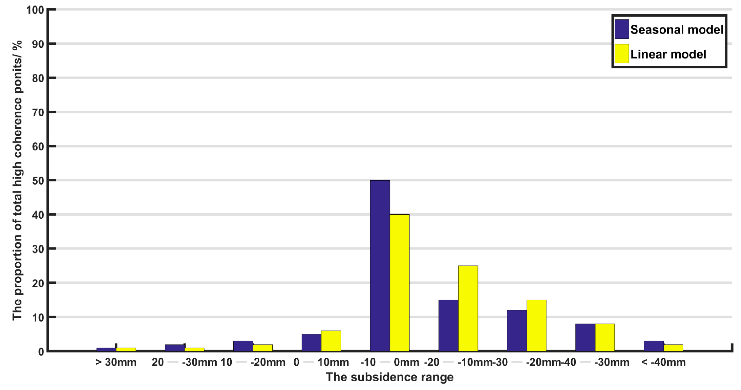
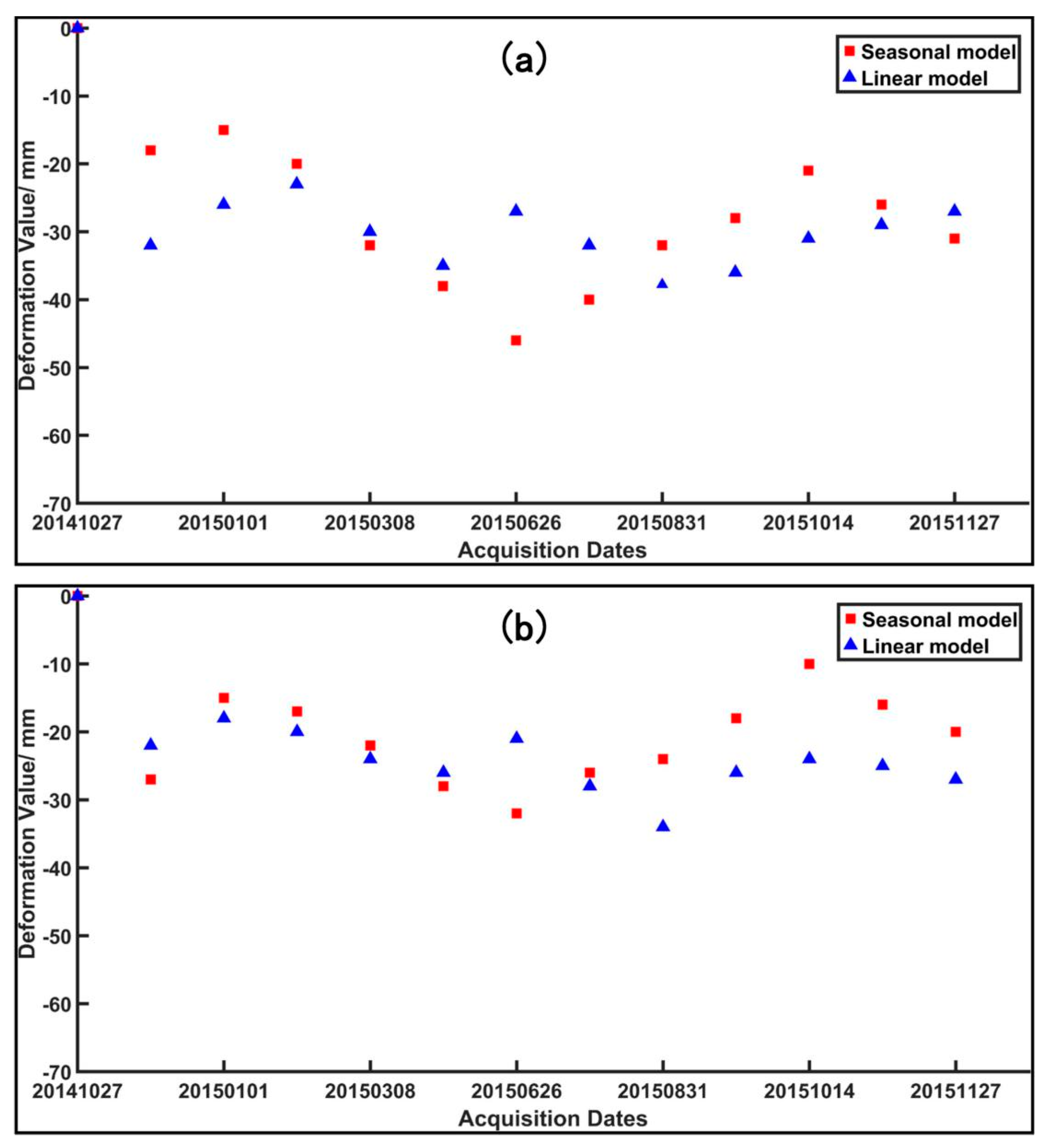
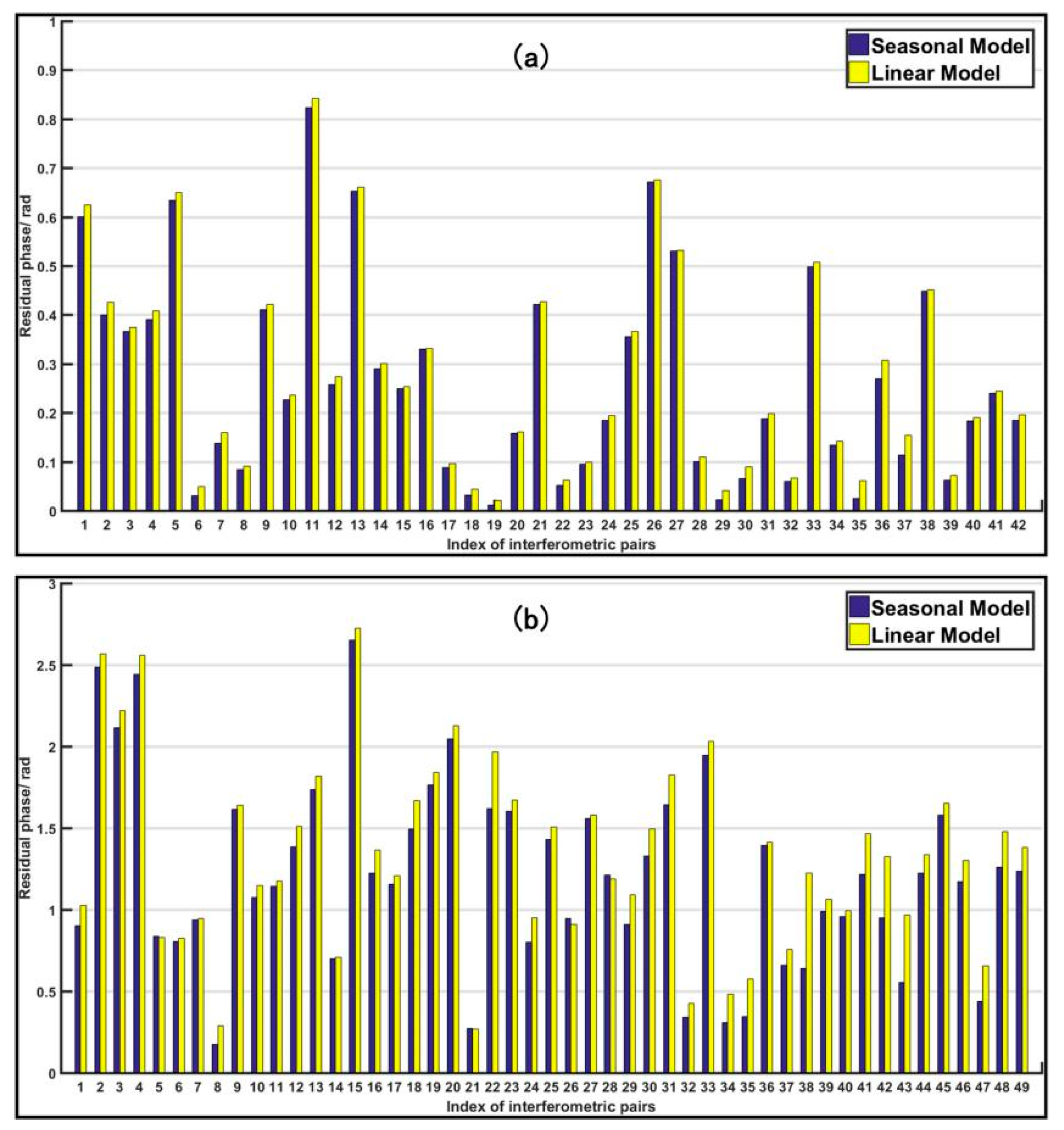
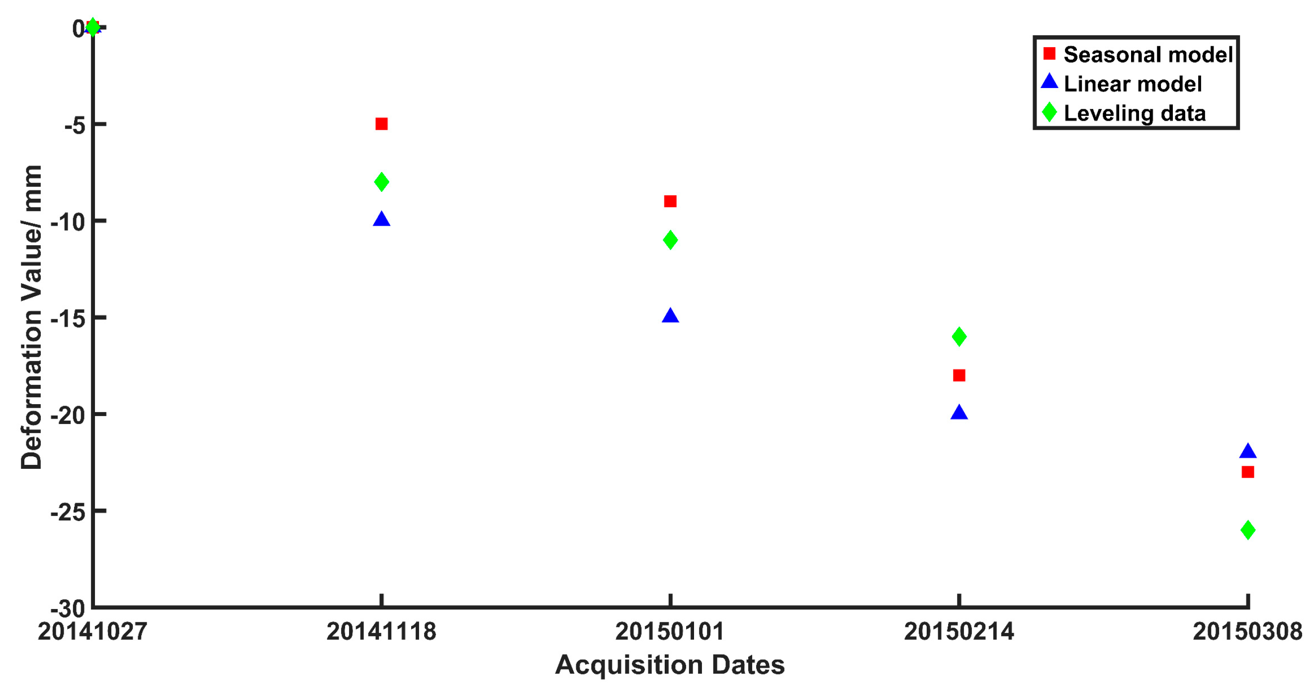
4.3. Accuracy Assessment
5. Conclusion
Author Contributions
Funding
Acknowledgments
Conflicts of Interest
References
- Bergado, D.T.; Ahmed, S.; Sampaco, C.L.; Balasubramaniam, A.S. Settlements of Bangna-Bangpakong highway on soft Bangkok clay. J. Geotech. Eng. 1990, 116, 136–155. [Google Scholar] [CrossRef]
- Shi, X.; Liao, M.S.; Teng, W.; Lu, Z.; Wei, S.; Wang, C.J. Expressway deformation mapping using high-resolution TerraSAR-X images. Remote Sens. Lett. 2014, 5, 194–203. [Google Scholar] [CrossRef]
- Mousavi, S.M.; Shamsai, A.; Naggar, M.H.E.; Khamehchian, M. A GPS-based monitoring program of land subsidence due to groundwater withdrawal in Iran. Can. J. Civ. Eng. 2001, 28, 452–464. [Google Scholar] [CrossRef]
- Lanari, R.; Mora, O.; Manunta, M.; Mallorqui, J.J. A small-baseline approach for investigating deformations on full-resolution differential SAR interferograms. IEEE Trans. Geosci. Remote Sens. 2004, 42, 1377–1386. [Google Scholar] [CrossRef]
- Berardino, P.; Fornaro, G.; Lanari, R.; Sansosti, E. A new algorithm for surface deformation monitoring based on small baseline differential SAR interferograms. IEEE Trans. Geosci. Remote Sens. 2003, 40, 2375–2383. [Google Scholar] [CrossRef]
- Chen, J.; Zeng, Q.M.; Jiao, J.; Zhao, B.C. SBAS time series analysis technique based on Sentinel-1A TOPS SAR images: A case study of Yellow River Delta. Remot. Sens. Land Resour. 2017, 29, 82–87. (In Chinese) [Google Scholar] [CrossRef]
- Lanari, R.; Berardino, R.; Bonano, M.; Casu, F.; Luca, C.D.; Elefante, S.; Fusco, A.; Manunta, M.; Manzo, M.; Ojha, C. Sentinel-1 results: SBAS-DInSAR processing chain developments and land subsidence analysis. In Proceedings of the 2015 IEEE International Geoscience and Remote Sensing Symposium (IGARSS), Milan, Italy, 26–31 July 2015. [Google Scholar]
- Corsetti, M.; Fossati, F.; Manunta, M.; Marsella, M. Advanced SABS- DInSAR technique for controlling large civil infrastructures: an application to the genzano di lucania dam. Sensors 2018, 18, 2371. [Google Scholar] [CrossRef] [PubMed]
- Papoutsis, I.; Papanikolaou, X.; Floyd, M.; Ji, K.H.; Kontoes, C.; Zacharis, V. Mapping infation at Santorini volcano, Greece, using GPS and InSAR. Geophys. Res. Lett. 2013, 40, 267–272. [Google Scholar] [CrossRef]
- Hooper, A.; Bekaert, D.; Spaans, K.; Arikan, M. Recent advances in SAR interferometry time series analysis for measuring crustal deformation. Tectonophysics 2011, 514, 1–13. [Google Scholar] [CrossRef]
- Tolomei, C.; Taramelli, A.; Moro, M.; Saroli, M.; Aringoli, D.; Salvi, S. Analysis of the deep-seated gravitational slope deformations over Mt. Frascare (Central Italy) with geomorphological assessment and DInSAR approaches. Geomorphology 2013, 201, 281–292. [Google Scholar] [CrossRef]
- Zhi, W.L.; Yang, Z.F.; Jian, J.Z.; Hu, J.; Yun, J.W.; Pei, X.L.; Guo, L.C. Retrieving three-dimensional displacement fields of mining areas from a single InSAR pair. J. Geod. 2015, 89, 17–32. [Google Scholar] [CrossRef]
- Solari, L.; Ciampalini, A.; Raspini, F.; Bianchini, S.; Zinno, I.; Bonano, M.; Casagli, N. Combined use of C-and X-Band SAR data for subsidence monitoring in an urban area. Geosciences 2017, 7, 21. [Google Scholar] [CrossRef]
- Han, Y.F.; Song, X.G.; Shan, X.J.; Qu, C.Y.; Wang, C.S.; Guo, L.M.; Zhang, G.F.; Liu, Y.H. Deformation monitoring of Changbaishan Tianchi volcano using D-InSAR technique and error analysis. Chin. J. Geophys. 2010, 53, 1571–1579. [Google Scholar] [CrossRef]
- Goldstein, R.M.; Engelhardt, H.; Kamb, B.; Frolich, R.M. Satellite radar interferometry for monitoring ice sheet motion: Application to an antarctic ice stream. Science 1993, 262, 1525–1530. [Google Scholar] [CrossRef] [PubMed]
- Li, J.; Li, Z.W.; Ding, X.L.; Wang, Q.J.; Zhu, J.J.; Wang, C.C. Investigating mountain glacier motion with the method of SAR intensity-tracking: Removal of topographic effects and analysis of the dynamic patterns. Earth Sci. Rev. 2014, 138, 179–195. [Google Scholar] [CrossRef]
- Xu, W.B.; Bürgmann, B.; Li, Z.W. An improved geodetic source model for the 1999 Mw 6.3 Chamoli earthquake, India. Geophys. J. Int. 2016, 205, 236–242. [Google Scholar] [CrossRef]
- Mirzaee, S.; Motagh, M.; Akbari, B.; Wetzel, H.; Roessner, S. Evaluating three InSAR time-series methods to assess creep motion, Case study: Masouleh landslide in North Iran. ISPRS Ann. Photogramm. Remote Sens. Spat. Inf. Sci. 2017, 223–228. [Google Scholar] [CrossRef]
- Bayer, B.; Simoni, A.; Schmidt, D.; Bertello, L. Using advanced InSAR techniques to monitor landslide deformations induced by tunneling in the Northern Apennines, Italy. Eng. Geol. 2017, 226, 20–32. [Google Scholar] [CrossRef]
- Sun, Q.; Zhang, L.; Ding, X.L.; Hu, J.; Li, Z.W.; Zhu, J.J. Slope deformation prior to Zhouqu, China landslide from InSAR time series analysis. Remote Sens. Environ. 2015, 156, 45–57. [Google Scholar] [CrossRef]
- Wang, C.; Zhang, Z.; Zhang, H.; Wu, Q.; Zhang, B.; Tang, Y. Seasonal deformation features on Qinghai-Tibet railway observed using time-series InSAR technique with high-resolution TerraSAR-X images. Remote Sens. Lett. 2017, 8, 1–10. [Google Scholar] [CrossRef]
- Zhao, R.; Li, Z.W.; Feng, G.C.; Wang, Q.J.; Hu, J. Monitoring surface deformation over permafrost with an improved SBAS-InSAR algorithm: With emphasis on climatic factors modeling. Remote Sens. Environ. 2016, 184, 276–287. [Google Scholar] [CrossRef]
- Lundgren, P.; Usai, S.; Sansosti, E.; Lanad, R.; Tesauro, M.; Fornaro, G.; Berardino, P. Modeling surface deformation observed with Synthetic Aperture Radar Interferometry at Campi Flegrei Caldera. J. Geophys. Res. 2001, 106, 19355–19366. [Google Scholar] [CrossRef]
- Usai, S. A least-squares approach for long-term monitoring of deformations with differential SAR interferometry. In Proceedings of the IEEE International Geoscience & Remote Sensing Symposium, Toronto, ON, Canada, 24–28 June 2002. [Google Scholar]
- Béjar-Pizarro, M.; Ezquerro, P.; Herrera, G.; Tomás, R.; Guardiola-Albert, C.; Hernández, J.M.; Merodo, J.F.; Marchamalo, M.; Martinez, R. Mapping groundwater level and aquifer storage variations from InSAR measurements in the Madrid aquifer, Central Spain. Hydrogol. J. 2017, 547, 678–689. [Google Scholar] [CrossRef]
- Lauknes, T.R.; Howard, A.Z.; Yngvar, L. InSAR deformation time series using an L1-Norm small-baseline approach. IEEE Trans. Geosci. Remote Sens. 2011, 49, 536–546. [Google Scholar] [CrossRef]
- Lanari, R.; Casu, F.; Manzo, M.; Lundgren, P. Application of the SBAS-DInSAR technique to fault creep: A case study of the Hayward fault, California. Remote Sens. Environ. 2007, 109, 20–28. [Google Scholar] [CrossRef]
- Manunta, M.; Marsella, M.; Zeni, G.; Sciotti, M.; Atzori, S.; Lanari, R. Two-scale surface deformation analysis using the SBAS-DInSAR technique: A case study of the city of Rome, Italy. Int. J. Remote Sens. 2008, 29, 1665–1684. [Google Scholar] [CrossRef]
- Arangio, S.; Calò, F.; Mauro, M.D.; Bonano, M.; Marsella, M.; Manunta, M. An application of the SBAS-DInSAR technique for the assessment of structural damage in the city of Rome. Struct. Infrastruct. Eng. 2014, 10, 1469–1483. [Google Scholar] [CrossRef]
- Zhou, L.; Guo, J.; Hu, J.; Li, J.; Xu, Y.; Pan, Y.; Shi, M. Wuhan surface subsidence analysis in 2015-2016 based on Sentinel-1a data by SBAS-InSAR. Remote Sens. 2017, 9, 982. [Google Scholar] [CrossRef]
- Li, S.S.; Li, Z.W.; Hu, J.; Sun, Q.; Yu, X.Y. Investigation of the seasonal oscillation of the permafrost over Qinghai-Tibet Plateau with SBAS-InSAR algorithm. Chin. J. Geophys. 2013, 56, 1476–1486. (In Chinese) [Google Scholar]
- Kampes, B.M.; Hanssen, R.F. Ambiguity resolution for permanent scatterer interferometry. IEEE Trans. Geosci. Remote Sens. 2004, 42, 2446–2453. [Google Scholar] [CrossRef]
- Funning, G.J.; Bürgmann, R.; Ferretti, A.; Novali, F.; Fumagalli, A. Creep on the Rodgers Creek Fault, northern San Francisco Bay area from a 10 year PS-InSAR dataset. Geophys. Res. Lett. 2007, 34, 255–268. [Google Scholar] [CrossRef]
- Ferretti, A.; Fumagalli, A.; Novali, F.; Prati, C.; Rocca, F.; Rucci, A. A New Algorithm for Processing Interferometric Data-Stacks: SqueeSAR. IEEE Trans. Geosci. Remote Sens. 2011, 49, 3460–3470. [Google Scholar] [CrossRef]
- Salichon, J.; Delouis, B.; Lundgren, P.; Giardini, M.; Costantini, M.; Rosen, P. Joint inversion of broadband teleseismic and interferometric synthetic aperture radar (InSAR) data for the slip history of the Mw = 7.7, Nazca ridge (Peru) earthquake of 12 November 1996. J. Geophys. Res.-Solid Eaeth 2003, 108. [Google Scholar] [CrossRef]
- Costantini, M.; Rosen, P.A. Generalized phase unwrapping approach for sparse data. In Proceedings of the IEEE International Geoscience & Remote Sensing Symposium, Hamburg, Germany, 28 June–2 July 1999. [Google Scholar]
- Xing, X.M.; Wen, D.; Chang, H.-C.; Chen, L.F.; Yuan, Z.H. Highway deformation monitoring based on an integrated CRInSAR algorithm—Simulation and real data validation. Int. J. Pattern Recognit. Artif. Intell. 2018, 32. [Google Scholar] [CrossRef]
- Roberto, T.; Yolanda, M.; Lopez-Sanchez, J.M.; José, D.; Blanco, P.; Jordi, J.M. Mapping ground subsidence induced by aquifer overexploitation using advanced Differential SAR Interferometry: Vega media of the Segura River (SE Spain) case study. Remote Sens. Environ. 2005, 98, 269–283. [Google Scholar] [CrossRef]
- Burbey, T.J. The influence of Geologic Structures on Deformation due to Ground Water Withdrawal. Ground Water 2008, 46, 202–211. [Google Scholar] [CrossRef]
- Hoffmann, J.; Zebker, H.A.; Galloway, D.L.; Amelung, F. Seasonal subsidence and rebound in Las Vegas Valley, Nevada, observed by synthetic aperture radar interferometry. Water Resour. Res. 2001, 37, 1551–1566. [Google Scholar] [CrossRef]
- Bell, J.W.; Amelung, F.; Ferretti, A.; Bianchi, M.; Novali, F. Permanent Scatterer InSAR reveals seasonal and long-term aquifer-system response to groundwater pumping and artificial recharge. Water Resour. Res. 2008, 44. [Google Scholar] [CrossRef]
- Wroblicky, G.J.; Campana, M.E.; Valett, H.M.; Dahm, C.N. Seasonal variation in Surface-subsurface water exchange and Lateral Hyporheic area of two stream-aquifer system. Water Resour. Res. 1998, 34, 317–328. [Google Scholar] [CrossRef]
- Segal, D.C.; Moran, J.E.; Visser, A.; Singleton, M.J.; Esser, B.K. Seasonal variation of high elevation groundwater recharge as indicator of climate response. J. Hydrol. 2014, 519, 3129–3141. [Google Scholar] [CrossRef]
- Hanssen, R.F. Radar Interferometry: Data Interpretation and Error Analysis; Kluwer Academic Publishers: New York, NY, USA, 2001. [Google Scholar]


| Image No. | Acquisition Dates (yyyy/mm/dd) | Normal Baseline (m) | Temporal Baseline (days) |
|---|---|---|---|
| 0 | 2014/10/27 | −126.22 | 242 |
| 1 | 2014/11/18 | 48.62 | 220 |
| 2 | 2015/01/01 | 122.99 | 176 |
| 3 | 2015/02/14 | −10.34 | 132 |
| 4 | 2015/03/08 | 15.94 | 110 |
| 5 | 2015/05/13 | −148.94 | 44 |
| 6 | 2015/06/26 | 0 | 0 |
| 7 | 2015/08/09 | −27.10 | 44 |
| 8 | 2015/08/31 | 57.39 | 66 |
| 9 | 2015/09/22 | −130.33 | 88 |
| 10 | 2015/10/14 | −36.83 | 110 |
| 11 | 2015/11/05 | −111.08 | 132 |
| 12 | 2015/11/27 | 111.41 | 154 |
| Deformation Model | Subsidence Increasing Period (yyyy/mm/dd) | Subsidence Decreasing Period (yyyy/mm/dd) | Maximum Subsidence (mm) | Maximum Fluctuation (mm) |
|---|---|---|---|---|
| Linear model | 2014/11/18–2015/08/31 2015/11/05–2015/11/27 | 2015/08/31–2015/11/05 | −71 (2015/08/31) | 67 |
| Seasonal model | 2014/11/18–2015/06/26 2015/09/22–2015/11/27 | 2015/06/26–2015/09/22 | −66 (2015/06/26) | 62 |
© 2019 by the authors. Licensee MDPI, Basel, Switzerland. This article is an open access article distributed under the terms and conditions of the Creative Commons Attribution (CC BY) license (http://creativecommons.org/licenses/by/4.0/).
Share and Cite
Zhu, Y.; Xing, X.; Chen, L.; Yuan, Z.; Tang, P. Ground Subsidence Investigation in Fuoshan, China, Based on SBAS-InSAR Technology with TerraSAR-X Images. Appl. Sci. 2019, 9, 2038. https://doi.org/10.3390/app9102038
Zhu Y, Xing X, Chen L, Yuan Z, Tang P. Ground Subsidence Investigation in Fuoshan, China, Based on SBAS-InSAR Technology with TerraSAR-X Images. Applied Sciences. 2019; 9(10):2038. https://doi.org/10.3390/app9102038
Chicago/Turabian StyleZhu, Yikai, Xuemin Xing, Lifu Chen, Zhihui Yuan, and Pingying Tang. 2019. "Ground Subsidence Investigation in Fuoshan, China, Based on SBAS-InSAR Technology with TerraSAR-X Images" Applied Sciences 9, no. 10: 2038. https://doi.org/10.3390/app9102038
APA StyleZhu, Y., Xing, X., Chen, L., Yuan, Z., & Tang, P. (2019). Ground Subsidence Investigation in Fuoshan, China, Based on SBAS-InSAR Technology with TerraSAR-X Images. Applied Sciences, 9(10), 2038. https://doi.org/10.3390/app9102038