Article

Evaluating the Energy Efficiency of Intermodal Trains

by
Mariusz Brzeziński
1,*,
Dariusz Pyza
1 and
Joanna Archutowska
2
1
Faculty of Transport, Warsaw University of Technology, Koszykowa 75, 00-662 Warsaw, Poland
2
Collegium of Business Administration, Warsaw School of Economics, Al. Niepodległości 162, 02-554 Warsaw, Poland
*
Author to whom correspondence should be addressed.
Appl. Sci. 2026, 16(7), 3567; https://doi.org/10.3390/app16073567
Submission received: 3 March 2026 / Revised: 1 April 2026 / Accepted: 3 April 2026 / Published: 6 April 2026
(This article belongs to the Special Issue Research Advances in Rail Transport Infrastructure)

Abstract

This article examines the impact of intermodal wagon technical specifications and railway infrastructure parameters on electricity consumption in rail freight transport. For this purpose, a three-stage analytical model was developed. The first stage defines the core assumptions, including train length, rolling stock types, container configurations, infrastructure constraints, and the characteristics of the energy consumption model. The second stage identifies the technical constraints of specific wagons, determines representative train compositions, and performs loading simulations. The third stage evaluates energy efficiency across different loading scenarios. The case study shows that specific energy consumption varies significantly with wagon type, train mass, and route characteristics. This findings challenge the use of static energy consumption values commonly applied in the literature. The results indicate that 40-foot wagons incur high energy penalties due to their tare weight and axle count, despite offering high loading capacity. While 60-foot wagons consume less energy, they lead to a high share of empty slots under a 20 t/axle limit. In contrast, 80-foot wagons are the most energy-efficient, particularly at a 22.5 t/axle limit. Mixed consists provide a balance between operational flexibility and competitive performance. Extending train length from 600 m to 730 m increases volume but does not automatically reduce unit energy consumption. These findings highlight the need to align wagon fleet selection with infrastructure capabilities and cargo characteristics. This study therefore provides practical recommendations for planning energy-efficient intermodal operations.

1. Introduction

The primary objective of this study is to develop a method that supports intermodal operators in optimising container transport for energy efficiency. Empirical observations suggest that energy efficiency increases significantly with improved railway infrastructure parameters, the selection of an appropriate wagon fleet, and an optimised loading strategy.
Intermodal transport includes, inter alia, the carriage of containers, semi-trailers, swap bodies and road-vehicle combinations. The core principle of intermodal transport is the movement of these ITUs (Intermodal Transport Units) using at least two different transport modes, without transshipping the cargo itself [1,2].
European Union (EU) Member States, in shaping sustainable development policy, support the growth of intermodal transport by introducing legal frameworks that facilitate its operation and enhance its competitiveness relative to conventional road transport [3]. An example of such regulations can be found in the TEN-T (Trans-European Transport Network) and AGTC (European Agreement on Important International Combined Transport Lines and Related Installations) agreements. These require the signatories, inter alia, to extend loading tracks at intermodal terminals and handover stations to 740 m, to increase the permissible axle load for freight traffic to 22.5 t, and to electrify loading tracks so that they can be accessed by electric locomotives without the need to use diesel traction [4]. Member States actively provide financial support for the construction of new intermodal transport infrastructure and handling equipment [5,6]. As noted by Kowalski [5], EU funding instruments have significantly supported the development of intermodal infrastructure, particularly in countries such as Poland, enabling terminal modernisation and improved rail connectivity. Recent findings reported by UIC [6] confirm the growing role of combined transport in Europe and emphasise its importance for decarbonisation, as well as the need for continued investment in infrastructure and technology.
Despite these advancements, discussions of sustainable development in intermodal transport rarely address the energy efficiency of intermodal rail freight. In particular, the academic literature does not sufficiently examine how wagon fleet selection and railway infrastructure parameters affect energy consumption. The only study analysing the impact of wagon configuration on energy consumption is presented in [7]. However, it focuses primarily on CO2 emissions, considering train length and the types of wagons used. Most of the available literature examines the energy consumption of trains composed of homogeneous wagon sets, typically dedicated to bulk freight [8], passenger transport [9,10], or intermodal transport [11,12].
On the one hand, railway lines used by intermodal trains differ in axle-load limits and maximum permitted train length. On the other hand, intermodal wagons available on the market vary in tare weight, length, and capacity, which allows them to carry containers of different sizes and gross weights.
These factors raise fundamental questions about how loading should be organised, which wagons should be used, and which parameters should be considered when selecting a railway route for transporting intermodal transport units in order to reduce energy intensity while maximising the number of containers or the total cargo mass carried. To address these issues, a three-stage research model was developed. Stage 1 defines the input assumptions, which largely determine the final results. In Stage 2, the basic constraints for the analysed wagon fleet are expressed as formulae. Train consists with both homogeneous and heterogeneous structures are then assembled, forming the basis for the loading scenarios developed in the next step; this stage concludes with a simulation of train loading under these scenarios. Stage 3 analyses the energy efficiency of intermodal transport on a given route.
The results highlight several key findings. First, longer trains do not always yield benefits. For some wagon types, unit energy consumption is higher in longer than in shorter consists. This is driven by, among other factors, greater wagon tare weight and a higher number of axles, which increase rolling resistance at the wheel–rail interface. Second, the case for 40-foot, four-axle wagons weakens as the permissible axle load increases from 20 to 22.5 t/axle. Because 60- and 80-foot wagons have a lower tare weight, they can become more economical as higher axle loads allow better use of their payload capacity. Third, the use of fixed unit energy consumption values in rail freight, often found in the literature, is not justified. These values vary with train gross mass, route length, wagon type, train length, permissible axle load, and other operational factors. Moreover, definitions of energy consumption per t-km are inconsistent across authors. Most do not specify how mass is defined in this unit, for example, whether it refers to train gross mass or net cargo mass.
This paper is structured as follows: Section 2 discusses the research findings in the field; Section 3 outlines the research algorithm; Section 4 presents a numerical example based on the research model; Section 5 interprets the results; and Section 6 provides general conclusions.

2. Literature Review

The production, storage, and distribution of energy pose substantial challenges for energy system operators, as well as for society and the environment. These processes are often associated with significant costs and greenhouse gas emissions [13,14]. In light of ongoing climate change and the potential for rising global energy prices, increasing attention is being directed towards the development of solutions that support energy conservation and efficient energy management [15,16,17]. Moreover, rising energy market volatility and decarbonisation goals have strengthened the role of technologies such as energy storage, which support system flexibility and facilitate the integration of renewable energy sources [15]. In this context, energy efficiency in the transport sector is of critical importance, as it remains one of the most energy-intensive sectors of the economy. Modern energy management is increasingly supported by forecasting and digital tools, which enable better alignment of energy supply and demand and improve operational efficiency [16]. In the railway sector, additional efficiency gains can be achieved through optimised energy use, monitoring systems, and data-driven management practices, as demonstrated in case studies of rail freight operations [17].
Importantly, reductions in energy consumption can be achieved not only through conventional measures, such as route optimisation, but also through less apparent strategies, including the optimal selection of transport modes and loading strategies for freight transport [18,19]. These aspects are further illustrated using the example of intermodal transport.
The literature review is divided into three parts. The first part examines global trends related to the electrification of transport, including rail transport. The second part reviews methods for optimising the loading of intermodal trains, with particular attention given to their relationship with energy consumption. The final part analyses approaches used to estimate energy consumption in freight rail transport, one of which is implemented in the model presented in this paper.

2.1. Transport Electrification

In global transport reports, electrification has been identified as one of the fastest-progressing processes within the broader energy transition. Documents [20,21,22,23,24,25] emphasise that the electric vehicle segment is currently developing rapidly. According to the IEA World Energy Outlook 2025 [20] and the Electricity 2025 [21] report, this growth is driven by falling battery costs, supportive policy frameworks, and expanding charging infrastructure. Together, these factors have accelerated market uptake across multiple regions. At the beginning of 2020, it remained relatively marginal; however, only four years later it achieved a significant market share—particularly in the passenger car segment. This trend is further confirmed by the DNV Energy Transition Outlook [22] and the IRENA World Energy Transitions Outlook 2024 [23]. These reports indicate that the electrification of transport is a central pillar of global decarbonisation pathways and is expected to intensify in the coming decades. Electrification is also expanding beyond passenger cars. The REN21 Global Status Report 2025 [24] highlights that electrification is expanding into other transport segments, including buses; light commercial vehicles; and, gradually, heavy-duty transport. Moreover, Pulido-Sánchez et al. [25] highlight the material and energy implications of large-scale transport electrification, emphasising both its decarbonisation potential and the associated challenges related to resource demand and energy system integration.
In recent years, rapid growth in electric two- and three-wheelers has been observed, particularly in Asia, along with a growing—though slower—share of electric vehicles in freight, rail, and bus transport [22,24]. The studies reviewed anticipate a further acceleration of transport electrification in the period up to 2050/2060. Some reports [22,23,26] present projections according to which electric vehicles will begin to dominate the structure of the entire operating fleet by mid-century. Several analyses also foresee a substantial increase in electrification in heavy-duty transport, albeit with a delay compared to the light-duty segment and with a significant role played by hybrid solutions [22,26,27].
An important complement to this perspective is provided by reports dedicated to rail and intermodal transport prepared by the International Energy Agency, the International Union of Railways, the International Union for Road–Rail Combined Transport, and Europe’s Rail Joint Undertaking [6,28,29,30]. They consistently emphasise that rail transport already exhibits a high degree of electrification compared to other modes, which positions it as a structurally advantaged component of low-emission freight systems. The UIC Activity Reports [28,29] highlight ongoing progress in the electrification of railway networks, improvements in traction efficiency, and increasing integration of digital solutions supporting energy management. These documents present rail as a transport mode that already makes extensive use of electric energy and, owing to its low energy intensity and emissions, may play a key role in the decarbonisation of land-based freight transport. Additionally, the joint UIC-UIRR report on combined transport [6] underlines the growing importance of intermodal solutions, in which rail serves as the backbone of long-distance freight movements and effectively reduces emissions compared with unimodal road transport.
The energy transition in this sector is primarily associated with further electrification of railway lines, improvements in the energy efficiency of rolling stock, and the development of combined transport, in which rail assumes the most emission-intensive segments of supply chains. Macroeconomic analyses, such as the EY European Economic Outlook [30], further contextualise these developments. They link investments in rail infrastructure and intermodal logistics with broader decarbonisation strategies and the resilience of European supply chains.
These documents consistently demonstrate that rail freight transport is significantly less energy-intensive than road transport and, for comparable cargo volumes, consumes several times less energy overall. In the scenario analyses presented particularly in [28,29], reductions in transport energy consumption are achieved primarily through modal shift from road to rail, improvements in railway infrastructure parameters (such as line electrification), and the modernisation and enhancement of rolling stock performance. On the other hand, study [9] addresses reductions in energy consumption in rail transport through decreasing the tare mass of freight wagons. It is shown that a lower wagon tare mass reduces the resistance forces that must be overcome to accelerate a freight train over a given section of a route. Lower resistance forces consequently result in lower energy consumption. The authors of [31] note that energy consumption varies depending on the type of wagons used; however, they do not examine the underlying causes of these differences. A technical analysis of energy consumption in rail freight transport is presented in [32]. This analysis considers route characteristics, wagon fleet and locomotive types, number of axles, train mass and length, operating speeds, axle loads, traction power supply systems, and related parameters. However, the study lacks a sensitivity analysis that would clearly show how total and unit energy consumption vary for a given scenario as individual parameters change.
Based on the literature review presented in this chapter, it can be concluded that there is a lack of practical knowledge on how to optimise freight train loading from a technical and operational perspective in order to reduce the energy intensity per unit mass of transported cargo. Moreover, the studies discussed do not provide specific quantitative values illustrating the extent to which energy consumption on the railway network may be reduced as a result of improvements in infrastructure parameters, such as increasing train length from 600 to 730 m or raising the permissible axle load from 20 to 22.5 t/axle.

2.2. Optimal Loading for an Intermodal Train

Among the few scholars to address this issue are those cited in [33]. The following conclusions can be formulated: (1) 40-foot and 80-foot wagons allow for the transport of the largest number of 40-foot containers; (2) 60-foot wagons are best suited to transporting 30-foot containers; (3) using 60- and 80-foot wagons allows transport of the greatest number of 20-foot containers.
In the international literature, optimal train loading is framed as the Train Load Planning Problem (TLPP). It is typically formulated with respect to criteria such as the following [34,35,36,37,38]: (1) minimisation of loading time; (2) optimal use of human and mechanical resources; (3) minimisation of train-loading costs; (4) optimal utilisation of the train’s loading length; and (5) minimisation of penalties for leaving cargo in the storage yard.
These objectives are often in conflict. This has led to the development of multi-objective optimisation approaches. For instance, Siri et al. [35] proposed models that explicitly balance operational efficiency and cost-related criteria. Similarly, Mantovani et al. [37] formulated the problem within a rigorous operations research framework, focusing on the combinatorial structure of container assignment, particularly in the context of double-stack intermodal trains.
Other studies focus on operational and simulation-based analyses. Kłodawski et al. [34] and Nehring et al. [36] investigated the impact of terminal operations and wagon configuration on loading time, highlighting the importance of practical constraints such as handling processes and equipment availability. In addition, Foti et al. [38] explored the use of Boolean optimisation techniques to solve large-scale TLPP instances efficiently, demonstrating the applicability of advanced computational methods.
In [39], the TLPP is defined as follows: a set of containers, differing in length, weight, loading priority, and stack position, must be assigned to wagons that vary in length, tare weight, and loading configurations. The objective is to determine an allocation that minimises the number of container-handling operations while maximising the number of loaded containers with the highest priority, subject to constraints on permissible length, payload capacity, and wagon loading configurations. The algorithm also enforces the permissible axle load—a key constraint determined by infrastructure parameters and the regulations of the railway infrastructure manager.
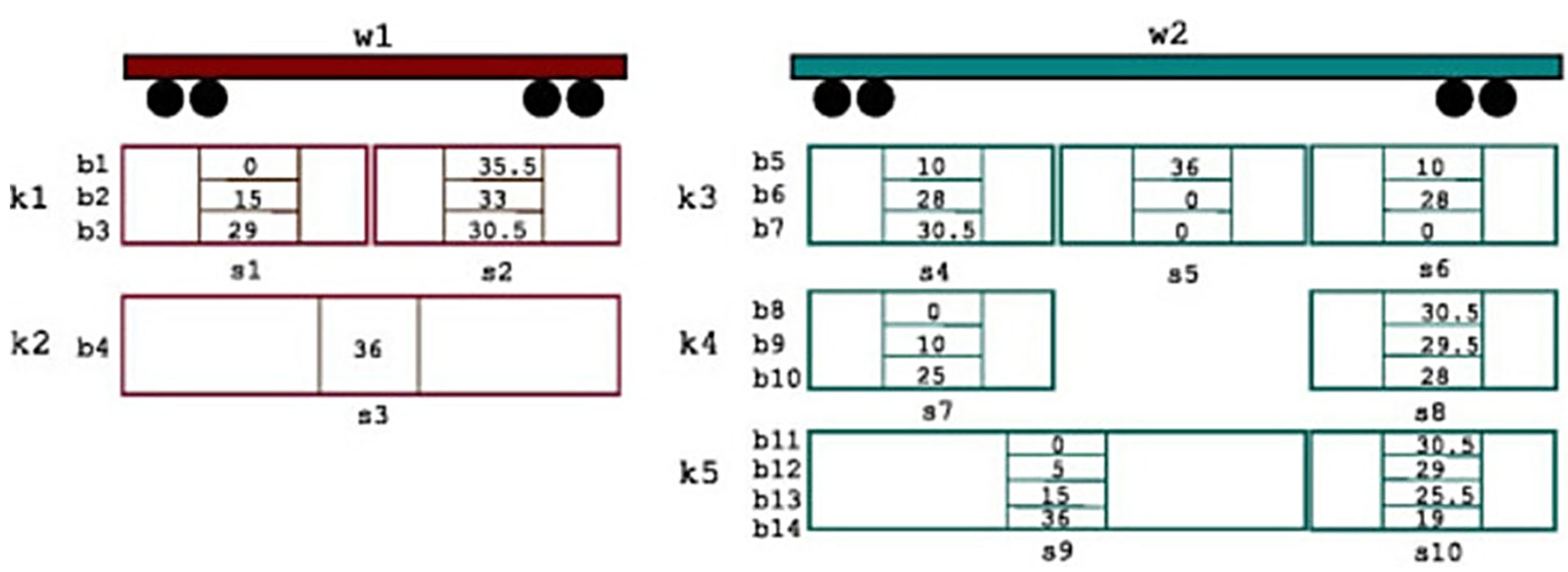
Figure 1 presents sample loading schemes for 40-foot and 60-foot wagons. These schemes show the maximum permissible container weight for each loading slot of a wagon.
Loading schemes also prevent overloading at either end of a wagon. This can occur when a very light container is placed at one end of the platform and a very heavy one at the other. In such cases, even if no bogie axle is overloaded, the wagon may tilt forward or backward, creating a safety hazard.
In practice, loading schemes are often insufficient, for example, when they are imprecise or offer too few configurations. In such situations, loading personnel use dedicated calculators to determine wagon axle loads. These calculations are based on basic equilibrium equations for statically and non-statically determinate beams [39].
In [39], the authors divide the optimal container-to-wagon assignment into two steps. First, they compute the maximum permissible container weight for each loading slot across wagon types. Second, they sort containers in descending order of weight. For each slot, the weight limit from the first step is compared with the heaviest available container in the yard. If it cannot be loaded, the process continues down the list until a container satisfies all constraints, including slot-specific limits and axle-load limits. Containers exceeding these limits are excluded from loading.
The TLPP has also been examined in numerous other publications [40,41,42]. In particular, Paul Corry and Erhan Kozan [40] formulated the train loading problem as an optimisation model that incorporates physical and operational constraints, such as wagon capacity and axle-load limits. Frank Bruns et al. [41] extended this approach by introducing robustness into the load planning process. They accounted for uncertainty in container weights and availability. Davide Anghinolfi and Marco Paolucci [42] proposed a Lagrangian heuristic framework that enables the efficient solution of large-scale problem instances. These studies generally consider 20- and 40-foot containers, which account for around 80–90% of the container market [43]. A common feature of this body of work is its focus on four-axle rail wagons. Container placement on such wagons is relatively straightforward from an operational perspective, as they offer limited loading configurations and simple axle-load calculations. In contrast, six-axle platforms (80-foot wagons) present a more complex loading problem, both mathematically and mechanically.
To address this gap, the present study examines the optimisation of train consists comprising not only 40- and 60-foot four-axle wagons but also 80-foot six-axle wagons. Solving this problem is considerably more complex than the approaches described in the international literature and—as will be shown—requires a tailored strategy. The study investigates energy efficiency with respect to wagon fleet type, train length, permissible axle load, and other operational parameters and loading strategies. This represents a novel contribution, as energy consumption in intermodal freight can be expected to vary significantly with these factors.

2.3. Methods for Estimating Energy Consumption in Rail Freight Transport

Electricity consumption in rail freight can be assessed in two ways: empirically, using meter readings, or theoretically, using models that estimate consumption from formulae. Early methods from the 1970s and 1980s, described in [44,45], required only a limited number of inputs, such as line voltage, current, and motor configuration. For example, the model presented by Wardrop [44] in the MTRAIN User’s Manual focused on practical simulation tools for railway operations. It enabled users to estimate energy consumption with relatively low data requirements. Later studies, such as those by Lee and Sun [45], introduced simulation-based approaches to evaluate the energy-saving potential of different train operation strategies. These approaches incorporated more detailed representations of train dynamics.
Overall, these early contributions laid the foundation for contemporary energy consumption models. They established key relationships between technical parameters and energy use, despite relatively simplified assumptions and limited input data. More recent studies have refined these estimation methods. Several studies [46,47,48,49] note that train energy consumption may depend on factors such as:
  • Track parameters, such as curve radius, rail pad type (e.g., hard rubber, steel, and soft rubber), track form (e.g., continuously welded or jointed), ballast, and gradient.
  • Mechanical and physical parameters, including wheel radius, gear ratio, traction system efficiency, train length and frontal area, and wagon type.
  • Operational conditions, such as speed, acceleration, load, and the rotational inertia of moving parts.
  • External factors, including wind and climate, which may affect the slip ratio as well as other track- and vehicle-related elements.
  • The presence of multiple train fronts, which increase total aerodynamic drag.
  • Driver behaviour and driving style.
In subsequent years, growing attention to environmental protection led to the development of methods that link emissions to energy consumption. Notable approaches include the MEET method (Methodologies for Estimating Emissions from Transport) [50], ARTEMIS (Assessment and Reliability of Transport Emission Models and Inventory Systems) [51], ETW (EcoTransIT World) [52], and mesoscopic models [53]. Each of these methods is described in detail by Heinold in [12,54,55].
The MEET model uses emission functions that depend primarily on average speed and vehicle type. This makes it simpler but less accurate under dynamic traffic conditions [50]. The ARTEMIS method is a detailed, microscopic emission model based on real-world speed profiles and engine operation. It accounts for traffic conditions and vehicle characteristics, which allows for high accuracy but requires substantial data [51]. The ETW (Engine-to-Wheel) approach focuses only on emissions generated during vehicle operation, excluding fuel or energy production [52].
Mesoscopic models provide an intermediate solution. They combine features of macro- and microscopic approaches by incorporating specific transport parameters, such as cargo mass, road gradient, and type of propulsion, based on average values for route segments. This approach offers relatively high emission estimation accuracy while requiring less data than microscopic models [53].
Knowledge of energy consumption in rail transport was also comprehensively systematised in our previous publication [7], which informed both the research model and the case study. In that work, total energy consumption included not only the energy required to overcome rolling resistance, but also losses in the traction network and conversion losses in electricity generation. In the present study, these factors are not included, as unit CO2 emissions from electricity generation are not calculated.
The most important symbols required to estimate energy consumption in each method are listed in Table 1.
The main problem in the global literature is not the diversity of methods used to estimate energy consumption, but the way in which the results obtained using these methods are interpreted. In the international literature, unit values of energy consumption are usually expressed in kWh/tkm (or Wh/tkm) [33,56,57,58]. Yet it is often unclear what these metrics actually include, as in [33]. For example, it is not always specified whether they refer to the total train mass, including locomotives and wagons, as in [56,57,58], or only the cargo mass, as in [59]. Nor is it consistently indicated which wagon types are used, what operating speeds are assumed, or which routes are analysed. To ensure reliable and comparable results, energy consumption units must therefore be defined explicitly, either descriptively or by means of equations, as done in this article.

3. Materials and Methods

Railway wagon designs differ in terms of length, mass, number of bogies, and payload capacity. These parameters largely determine how effectively individual wagon types perform in specific transport tasks. They directly affect the degree of train utilisation, as well as its gross and net mass, and consequently the unit energy consumption per ITU/TEU and per tonne of gross or net cargo.
To illustrate these relationships quantitatively, it is necessary to simulate intermodal train loading while taking into account both wagon design constraints, such as payload capacity, and railway infrastructure parameters, particularly permissible axle loads. This also requires the formulation of appropriate models and mathematical relationships. The results of the study make it possible to demonstrate the potential for energy optimisation in rail intermodal transport, a topic that has not yet been examined in such detail in the international literature.
The research model comprises three stages:
Stage 1: Identification of input data—In this stage, the inputs to the research model were specified. These included wagon parameters, train length, railway line characteristics, container types and their gross weights. This stage also defines the method used to estimate energy consumption, as well as the operational parameters of the given train route. Some of these inputs determine the loading scenarios analysed in Stage 2 and have a significant impact on the results obtained in Stage 3.
Stage 2: Simulation of container train loading (container consist)—Stage 2 comprises four steps. In Step 1, constraints on the wagon fleet, including axle loads and bending moments, were identified and defined using physico-mechanical formulae. These were based on equilibrium equations for statically determinate beams in the case of four-axle 40- and 60-foot wagons and statically indeterminate beams for six-axle 80-foot wagons. In Step 2, a purpose-built solver was used to assemble train consists composed of different wagon types given a specified objective function and selected constraints. Alongside heterogeneous consists, homogeneous consists, which are the most common on the European market, were also analysed. In Step 3, loading scenarios were developed that varied by train length, axle load, and wagon type. Step 4 defined the assumptions and objective functions that may guide operators in loading an intermodal train. Containers were then allocated manually to wagons in each scenario using dedicated calculators.
Stage 3: Results analysis—In the final stage, the total and unit energy consumption for transporting a given set of containers under different loading scenarios were analysed. Based on these results, conclusions and recommendations for intermodal operators were formulated.
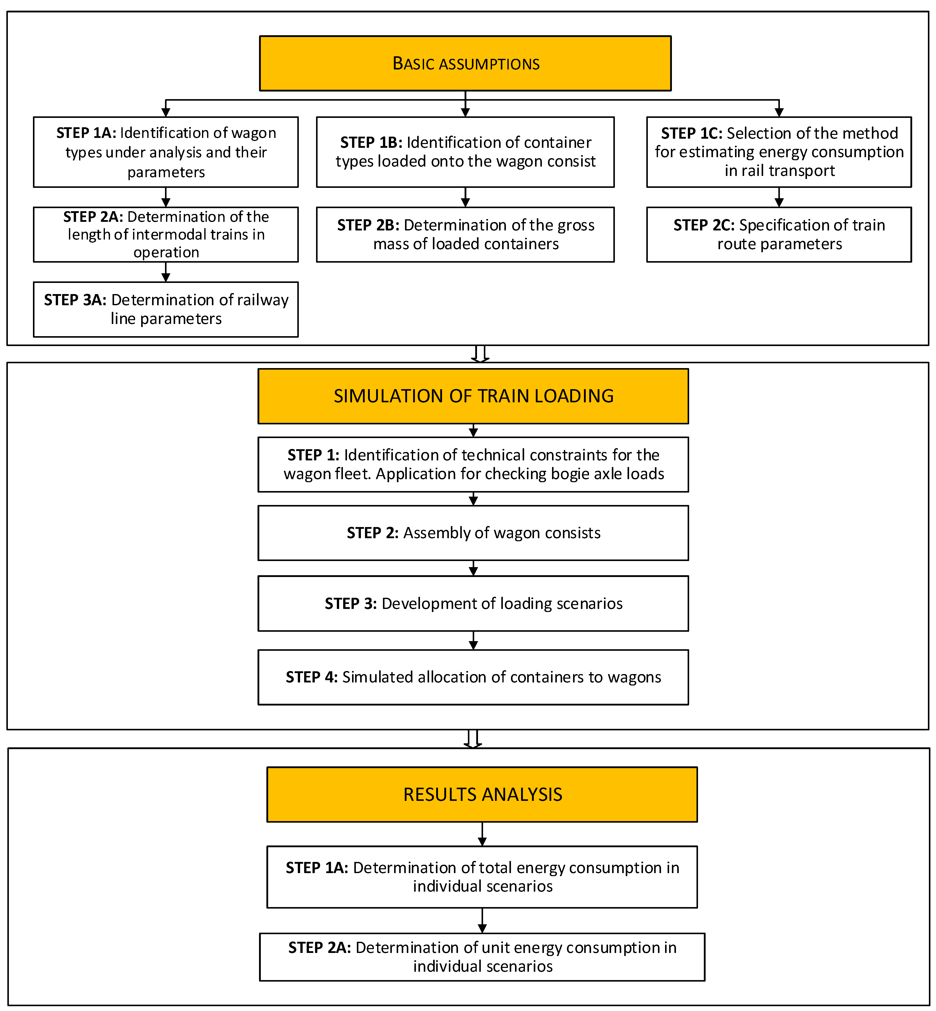
Figure 2 illustrates the research model.
Definition of the terms used in the above model is provided below:
Stage 1—Definition of the basic assumptions of the model
Step 1A: Identification of wagons and their parameters
The wagons used in intermodal transport are 40-, 60-, 80-, and 90-foot wagons. Their designations are presented as follows ( z ) : z = 1 :   40-foot wagon, z = 2 :   60-foot wagon, z = 3 :   80-foot wagon, and z = 4 :   90-foot wagon.
Step 2A: Determination of intermodal wagon consists
In Western and Central Europe, where the standard track gauge of 1435 mm prevails, two train lengths dominate in freight operations: 620 m and 750 m (or 740 m). The corresponding lengths of wagon consists are 600 m and 730 m, respectively. These lengths exclude the locomotive (~20 m).
Step 3A: Determination of railway line parameters
Railway lines on which freight trains operate are characterised by specific parameters. One such parameter is the permissible axle load that a wagon bogie axle may exert on the track. Until recently, most European railway infrastructure allowed freight trains to operate primarily with a maximum axle load of 20 t/axle. However, in line with the AGTC and TEN-T agreements, modernisation works are underway that are expected to enable trains to operate with an axle load of 22.5 t/axle on the main corridors of the European railway network. To distinguish between railway line classes ( f ), the following designations have been introduced: f = 1 : railway line with axle load up to 20 t/axle, f = 2 : railway line with axle load up to 22.5 t/axle, f = 3 : railway line with axle load up to 25 t/axle, and f = 4 : railway line with axle load up to 18 t/axle.
Step 1B: Identification of container types loaded onto the wagon consist
A wide variety of container sizes are used worldwide. These include containers with 10-, 20-, 30-, 40-, and 45-foot lengths. The following designations ( a ) have been introduced: a = 1 :   20-foot container, a = 2 :   40-foot container, a = 3 : 30-foot container, a = 4 :   10 - f o o t   c o n t a i n e r , and a = 5 :   45 - f o o t   c o n t a i n e r .
The sizes of the discussed containers have been identified as follows ( ϑ a ): ϑ 1 = 1   T E U ,     ϑ 2 = 2   T E U ,   ϑ 3 = 1.5   T E U ,     ϑ 4 = 0.5   T E U , and ϑ 5 = 2.25   T E U .
Step 2B: Determination of the gross mass of loaded containers
The gross weight of a container depends on its tare weight and the weight of the loaded cargo. The tare weight of a 20-foot container is approximately 2.2 t, while that of a 40-foot container is about 4.0 t. In both cases, around 26.0–28.0 t of cargo can be loaded. Therefore, the gross weight of a container of type a ( m a ) may be
m a = { [ 2.2 ,   30.2   ]   t ,   f o r   a = 1   [ 4.0 ,   32.0 ]   t ,   f o r   a = 2
Step 1C, 2C: Selection of the method for estimating energy consumption in rail transport and specification of train route parameters
At this stage, one of the methods described in the literature must be selected to estimate energy consumption in intermodal rail transport. For the chosen method, it is then necessary to identify the parameters that influence the energy use of an electrified intermodal train. In this analysis, one of the methods outlined in the literature review is selected.
Stage 2—Assembly of wagon consists and simulation of the loading process
Step 1: Determination of technical constraints for the wagon fleet
Rail vehicles are subject to technical constraints that must be observed during loading. During the loading of an intermodal train, dedicated loading schemes and calculation tools must be used. Loading schemes provide the operator responsible for loading with information on the permissible configurations for a given wagon. They indicate the positions of locking pins, which secure container corners and prevent containers from shifting or falling off the wagon during transport. For 20- and 40-foot containers, these locking pins are located in different positions depending on the wagon type. Loading schemes also specify the maximum allowable container weights for each loading configuration.
In the absence of loading schemes, loading calculators must be used to determine the load on individual wagon axles. The operator responsible for loading evaluates selected configurations using containers from the transport list. In practice, situations frequently arise in which axle overload occurs, for example, when two excessively heavy containers are assigned to the same wagon. In such cases, one of the containers must be replaced with a lighter unit.
To achieve optimal train loading, understood here as minimising empty slots while maximising net payload, containers should be arranged in descending order of weight. The loading process should begin with the heaviest containers and then be complemented with lighter ones so as to avoid exceeding axle-load limits. At the same time, the operator should minimise the number of unused loading slots on individual wagons.
In the case of a heterogeneous wagon composition, it is also advisable to begin loading the heaviest containers onto wagons with the most favourable loading characteristics, such as 40-foot four-axle wagons. Lighter containers should then be loaded at a later stage onto wagons with less favourable loading characteristics, such as 60-foot four-axle wagons, as this reduces the likelihood of exceeding axle-load limits.
The formal representation of the equations implemented in wagon loading calculators is presented below:
Constraint due to the wagon’s payload capacity limit
Each wagon has a specified payload capacity. Overloading can cause floor failure; therefore, the total mass of containers loaded on a wagon of type z must not exceed the manufacturer’s rated payload:
a A i I a m i , a · x i , k Y z 2   [ t ] ,     z Z , k Z k
where m i , a is the mass of the i - t h container of type a ; x i , k   is a binary decision variable equal to 1 if container i is assigned to wagon k and 0 otherwise (this variable determines whether the mass of the container is included in the load of wagon k ); and Y z 2 is the diagnostic variable denoting the payload capacity of a wagon of type z, expressed in [t].
Constraint due to the wagon’s maximum capacity
Each wagon type has a specified capacity expressed in TEU; accordingly, the total TEU-equivalent length of containers loaded on a wagon of type z must not exceed that wagon’s loading length.
a A i I a ϑ i , a · x i , k Y z 3   [ T E U ] ,     z Z , k Z k
where ϑ i , a is the TEU-equivalent length (e.g., 1 TEU for a 20-ft container and 2 TEU for a 40-ft container) of the i - t h container of type a and Y z 3 is the diagnostic variable denoting the capacity of a wagon of type z, expressed in TEU. The capacities of wagons may be defined as follows: Y 13 = 2   T E U ,   Y 23 = 3   T E U ,   Y 33 = 4   T E U   (where 1 TEU corresponds to the size of a 20-foot container).
Constraint due to the wagon’s permissible axle load
Railway tracks used by freight trains are designed with specific strength parameters. One of these is the permissible axle load that a wagon bogie axle may impose on the track. This constraint prevents excessive overstressing of the infrastructure and can be expressed as follows:
R j t z 2 α p e r f   [ t / a x l e ]
where R j t z is the load on the j t - t h bogie of a wagon of type z and α p e r f is the permissible axle load in railway line class f .
The value R j t z is determined differently for four-axle and six-axle wagons. For four-axle wagons, the following equations must be solved:
(a)
The equation for the vertical force equilibrium acting on the wagon between gravitational forces and track reaction forces:
  j t = 1 2 R j t z = j t = 1 2 T j t z + a A i I a m i , a ,     z = 1,2
where T j t z is the portion of the wagon’s tare mass assigned to each bogie in the z - t h type of wagon.
(b)
The bending moment distribution equations for the wagon:
( R j t z T j t z ) · c z a A i I a m i , a · b i , a z = 0                       z = 1,2 ,   j t = 2
where c z is the axle spacing of a wagon of type z and b i , a z is the distance from the support point ( R j t z ) to the center of gravity of the i - t h container of type a on a wagon of type z.
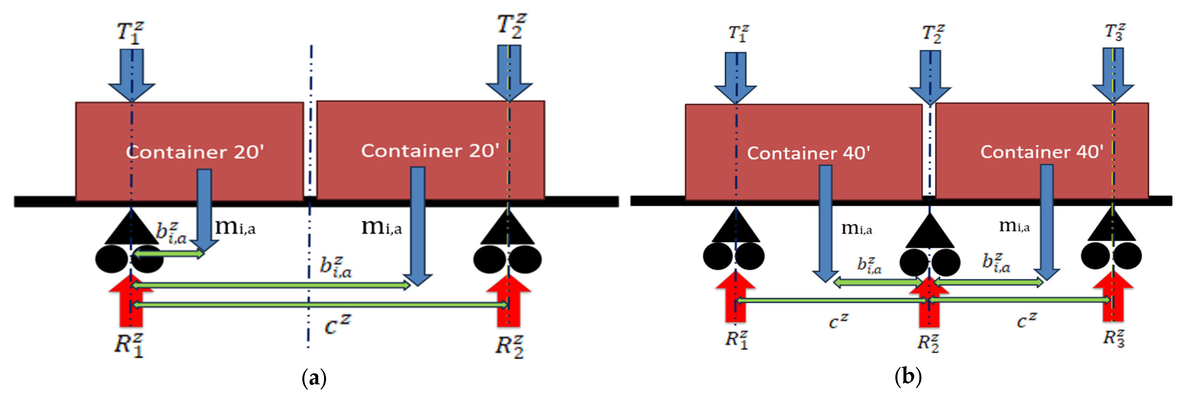
The designations used in the above equations are illustrated below (see Figure 3).
An 80-foot wagon is a statically indeterminate structure. To determine its support reactions, the wagon floor must be modelled as two independent statically determinate spans. For six-axle wagons, the following equations must therefore be solved:
(a)
The equation for the vertical force equilibrium acting on the wagon, i.e., gravitational forces and track reaction forces:
    j t = 1 3 R j t z = j t = 1 3 T j t z + a A i I a m i , a ,     z = 3
(b)
The bending moment distribution equations for the wagon:
  ( R j t z T j t z ) · c z a A i I a m i , a · b i , a z = 0 ,     z = 3 , j t = 1   ( R j t z T j t z ) · c z a A i I a m i , a · b i , a z = 0 ,     z = 3 , j t = 3
The designations used in the above equations are illustrated above (see Figure 3).
Step 2: Formation of wagon consists
Rail wagons used for container transport can be configured in two ways. In the first, the train consist is composed of a single wagon type—such formations are referred to as homogeneous consists. The number of wagons in a homogeneous consist is given by the following formula:
z Z   w z L H T Y z 4 [ u n i t s ]
where L H T is the length of the wagon consist and Y z 4 is the diagnostic variable denoting the length of a wagon of type z, expressed in [m].
Intermodal operators can also assemble consists from different wagon types; in this article, such formations are referred to as heterogeneous consists.
When assembling such a consist, the operator may pursue different objective functions, for example:
  • The operator may aim to minimise the total tare mass of all wagons (as infrastructure managers usually charge higher access fees for heavier trains) ( M w a g ) . This objective can be formulated as the minimisation of the total wagon mass, expressed as the sum of the products of the number of wagons of type z   ( z = 1 Z w z ) and the tare weight of a wagon of type z   ( Y z 1 ) .
  • The operator may select wagons for the consist so as to maximise their total payload capacity expressed in tonnes ( P L C ) , since a greater carried volume increases transport revenue. This objective can be formulated as the maximisation of the sum of the products of the number of wagons of type z   ( z = 1 Z w z ) and the payload capacity of a wagon of type z   ( Y z 2 ) .
  • The operator may select wagons for the consist so as to maximise their total capacity or the total number of slots expressed in TEU ( L G H ), as the more TEUs are transported, the greater the revenue that can be gained. This objective can be formulated as the maximisation of the total wagon capacity, expressed as the sum of the products of the number of wagons of type z   ( z = 1 Z w z ) and the capacity of a wagon of type z   ( Y z 3 ) .
  • The operator may seek an optimal solution that simultaneously accounts for all the above objective functions.
One of the above functions will be implemented in the solver.
It is important to ensure that, in order for the program to determine the number of wagons correctly, a constraint is imposed on the total length of all wagons, that is, the overall train consist length:
0 w z W M a x z ;   z w z · Y z 4 L H T   [ m ]
where W M a x z is the availability of wagons of type z.
Step 3: Determination of loading scenarios
Based on the previous step, loading scenarios can be defined that differ by the type and number of wagons used, train/consist length, and railway line class. The set of scenarios is denoted as
V = { v : v = 1 , V ¯ }
where v is the scenario index.
Step 4: Simulated assignment of wagons to the consist
Once the wagon fleet and its technical constraints are defined, the loading simulation can be performed. During loading, the entity responsible for container allocation may, for example, aim to achieve the following:
(a)
Maximise the utilisation of the loading space within the wagon consist ( U T ( v ) ) (same equation as (2)).
(b)
Transport the largest possible gross cargo mass ( M g o o d s g r o s s ( v ) ) (same equation as (1)) or transport the largest possible net cargo mass ( M g o o d s n e t ( v ) ) :
M g o o d s n e t ( v ) = z Z k K z a A i I a ( m i , a m i , a t a r e ) · x i , k , v M A X ,     v V
where m i , a t a r e is the tare mass of the i - t h container of type a selected for loading and x i , k , v is a binary decision variable equal to 1 if container i is assigned to wagon k in the v - t h scenario and 0 otherwise. This variable determines whether the mass of the container is included in the load of wagon k . This concerns the v - t h scenario.
Since no automated tool is available to perform the loading simulation in accordance with the above objective functions, the process must be carried out manually by analysing the loading of each wagon individually.
(c)
Minimising empty slots ( E S ( v ) ) within the wagon consist.
The number of empty slots, expressed in TEU, is defined as the difference between the maximum slots available in the consist under a given scenario, L G H ( v ) , and the actual number of slots utilised in that consist, U T ( v ) .
Stage 3—Analysis of results
Step 1A: Determination of total energy consumption
Once the loading simulation is complete, the train’s operational parameters can be compared. In the final stage, the comparison focuses on the total energy consumption of the locomotive(s) and the specific energy consumption for each scenario. The general equation for the total energy consumption of an intermodal train in the v - t h scenario, calculated using the n t - t h method ( E T T W n t ( v ) ) , is given below:
E T T W n t ( v ) = E n t ( v ) · 1 ϵ l o c [ k W h ]
where ϵ l o c is the electric locomotive engine efficiency and E 4 ( v ) is the energy required to overcome train resistances in the v - t h scenario.
For n t = 4 (mesoscopic method):
E 4 ( v ) = d V a v g · [ p A ( v ) + p T ( v ) + p G ( v ) + p A U X ( v ) ] + n s · d 100 · W t r ( v ) [ k W h ]
where d is the travelled distance, V a v g is the train average velocity, p A U X ( v ) is the power auxiliary devices (i.e., computers, lights, and air-conditioning in the locomotive) in the v - t h scenario, p A ( v ) is thepower required to overcome the aerodynamic drag of the locomotive and wagons in the v - t h scenario, p T ( v ) is the power required to overcome the rolling resistance of the locomotive and wagons in the v - t h scenario, p G ( v ) is the power required to overcome gradient resistance in the v - t h scenario, and n s is the number of stops. Further explanations of the remaining symbols are provided in references [7,51,54,55].
Step 2A: Determination of energy consumption
The total energy consumed by the train in a given loading scenario is not entirely informative, as it also includes the tare mass of the wagons. Therefore, to assess the energy use of the train more precisely, it is necessary to calculate the energy consumption in accordance with the formula described in [7], adapted for the purposes of this study:
  • Per gross train t-km ( F J g r o s s ( v ) ) :
F J g r o s s ( v ) = E T T W n t ( v ) d · M t l ( v )   [ k W h g r o s s t k m   ]
where M t l ( v ) is the gross mass of train in the v - t h scenario, or
  • Per net cargo t-km ( F J n e t ( v ) ) :
F J n e t ( v ) = E T T W n t ( v ) d · M g o o d s n e t ( v )   [ k W h n e t t k m   ]
or per TEU ( F J T E U ( v ) ) :
F J T E U ( v ) = E T T W n t ( v ) U T ( v )   [ k W h T E U   ]
or per ITU ( F J I T U ( v ) ) :
F J I T U ( v ) = E T T W n t ( v ) U T N ( v )   [ k W h I T U   ]
where U T N ( v ) is the number of ITUs loaded in the v - t h scenario.

4. Results

In the first subsection of this section, the impact of technical and operational factors on the energy consumption of intermodal trains is examined. The model incorporates real parameter values related to wagons, containers, and the train itself. Subsequently, loading scenarios are prepared in accordance with the principles defined in the model. These scenarios differ in terms of wagon composition and railway line parameters, particularly permissible axle loads; in this subsection, only trainsets with a length of 600 m are analysed.
In the following stage, a simulation of train loading is carried out for various scenarios, in accordance with the assumptions adopted in the model. The loading simulation, subject to the defined constraints, makes it possible to determine additional train parameters, such as gross train mass, net cargo mass, and the number of empty loading slots. Based on the selected energy consumption model, the input parameters, and the results obtained from the simulation, both total and unit energy consumption are calculated for successive loading scenarios.
At the end of the subsection, representative characteristics illustrating energy consumption and selected train operating parameters are presented, including the number of available slots, the gross train mass, and the number of loaded containers. This approach allows for the identification of relationships between energy consumption, operational practices, and the quality of the wagon fleet used.
In the second subsection, a comparative analysis is conducted in which scenarios involving 600 m long wagon consists are compared with those involving trains with a length of 730 m.
The results support the thesis that the energy consumption of electric trains depends not only on operating parameters, such as speed, gradient, and aerodynamic resistance, but also on factors such as wagon type, infrastructure parameters, and train length.

4.1. Algorithm Implementation, Calculations, and Results

Stage 1—Definition of the basic model assumptions
Stage 1 begins with the formulation of the model’s basic assumptions. These assumptions largely determine what is tested, how it is tested, and the results obtained in Stage 3. Depending on the selected wagon fleet and the container types used for transport, energy consumption and the utilisation of available loading space may vary.
In Step 1, 40-, 60-, and 80-foot wagons were selected for analysis. Ninety-foot wagons are less common in international intermodal transport due to the limited availability of 45-foot containers worldwide—these, together with 40-foot refrigerated containers equipped with cooling units, are typically the only units loaded onto such wagons. Consequently, this type of rolling stock was excluded from the analysis. Table 2 presents illustrative parameters for the 40-, 60-, and 80-foot wagons used in the analyses that follow. For the purposes of the analysis, the parameters of SGGRS wagons (80-foot wagons), SGS wagons (60-foot wagons), and SGMMNS wagons (40-foot wagons) were used.
In Step 2A, the length of the wagon consists to be formed was determined. To diversify the scenarios, the study included both consist lengths listed in the previous section. It is generally assumed that longer consists are more economical than shorter ones—a hypothesis tested in the sensitivity analysis.
In Step 3A, the class of railway lines on which the intermodal trains would operate was specified. Under the TEN-T Regulation, tracks should support an axle load of 22.5 t. However, lines limited to 20 t remain common. This constraint prevents the optimal use of wagon payload capacity, as it often leads to bogie-axle overloading. Lines allowing 25-tonne axle loads are relatively rare in Europe; accordingly, the analysis was confined to operations under 20- and 22.5-tonne axle-load conditions.
In Step 1B, 20- and 40-foot containers were selected for further analysis, as they are the most commonly used units in rail transport. Together, they account for approximately 90% (and up to 96% in Poland [61]) of all ITUs handled. The list of container types and their dimensions is presented in Table A1 in Appendix A.
In Step 2B, we specified the gross masses of the containers to be loaded. Values were generated in Excel using the RAND() function. The analysis focused on high-gross-mass containers, which are typically more difficult to load. Gross mass was sampled uniformly over 22–30 t (see Table A1 in Appendix A). Sampling also respected the constraint that the combined mass of the container and the road vehicle used in the road leg does not exceed the permissible limit for combined road transport (44 t) [62].
In Step 1C, the mesoscopic method discussed in [7] was selected for estimating the energy consumption of intermodal trains, as it had been previously implemented and validated.
In Step 2C, the train route parameters were specified. While velocity, trip altitude difference, distance, and number of stops were based on empirical experience, the remaining parameters were derived from values reported in [7,51,54,55]—see Table 3.
Stage 2—Simulation of intermodal train loading (train consist)
In Step 1, a dedicated tool was developed to calculate bogie-axle loads for a given container type during loading. It was implemented in MS Excel. For the tool to compute axle loads correctly, selected technical parameters of intermodal wagons had to be specified, as shown in Table 4.
In Step 2, wagon consists were assembled. Both homogeneous and heterogeneous consists were considered. Homogeneous consists were obtained by dividing the nominal train length by the length of a single wagon ( Y z 4 ). At this stage, only 600 m long wagon consists were considered. Mixed wagon consists were generated using the fourth function described in Section 4 (Stage 2, Step 2). The objective function in the solver was formulated to identify an optimal solution that accounts for all the above-mentioned objectives. It maximises the number of cargo slots and the wagon payload, while simultaneously minimising the total tare weight of the wagons.
In the case of homogeneous wagon consists, the intermodal operator is not constrained by the number of available wagons. It was therefore assumed that the operator had the following fleet available for service: W M a x 1 = 7 ,   W M a x 2 = 54 , and W M a x 3 = 15 .
In Step 3, based on the previous step, loading scenarios were developed that differed in terms of permissible axle load ( α p e r 1 = 20   t / a x l e and α p e r 2 = 22.5 t / a x l e ) and in the types of wagons used. As noted earlier, the case study analysis was carried out for wagon consists with an L H T = 600   m . After defining the scenarios, the tare mass of wagons, the total payload capacity in tonnes, the total capacity in TEU, and overall train length were analysed. For the purposes of sensitivity analysis, an analogous assessment was performed for L H T = 730   m (Table A2 in Appendix A)
In Step 4, a list of 82 containers was generated (Table A1 in Appendix A), consisting of 50 20-ft containers and 32 40-ft containers. Each unit was randomly assigned a gross mass within the range of 22–30 t, allowing for the simulation of container-to-wagon allocation. The adopted strategy prioritised the dispatch of containers with the highest loading priority; accordingly, containers were sorted in ascending order of priority value. Each intermodal transport unit was then manually allocated to wagons using a dedicated calculation tool. The results are summarised in Table A3 in Appendix A and include, among other indicators, the number of utilised slots within the train consist, the level of slot utilisation (in %), the payload utilisation ratio, the number of loaded 20- and 40-foot containers, and the gross and net mass of the loaded cargo.
Stage 3—Analysis of results
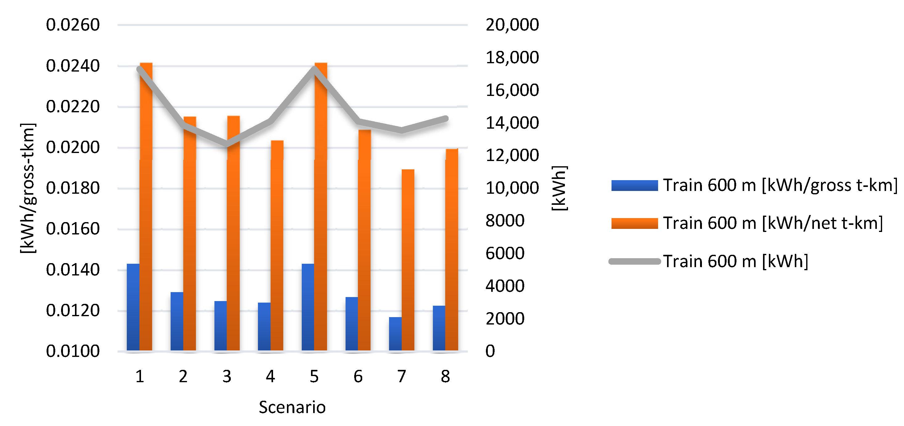
In Step 1A and Step 2A of Stage 3, the level of energy consumption for each scenario was determined in accordance with the procedure outlined in Section 3. To perform these calculations, the relevant input parameters were first prepared, as presented in Table 3. The results obtained are shown in Figure 4.
From the figure, it can be seen that total energy consumption in each scenario ranged from 12.7 to 17.3 MWh. The lowest value was observed in Scenario 3 (12.7 MWh), while the highest occurred in Scenarios 1 and 5 (both 17.3 MWh). Energy consumption per gross train t-km ranged from 0.012 to 0.014 kWh, with the lowest value in Scenario 7 (0.012 kWh/gross tkm) and the highest in Scenario 1 (0.014 kWh/gross tkm). Energy consumption per net cargo t-km ranged from 0.019 to 0.024 kWh, again with the lowest value in Scenario 7 (0.019 kWh/net tkm) and the highest in Scenarios 1 and 5 (0.024 kWh/net tkm).
The largest reduction in unit energy consumption, expressed in kWh/gross tkm and kWh/net tkm, was observed in scenarios using 80-foot wagons when the permissible axle load increased from 20 to 22.5 t/axle. In these cases, unit energy consumption was lower by 6% and 12%, respectively, compared with scenarios operating under a 20 t/axle limit. No such effect was observed for 40-foot wagons.
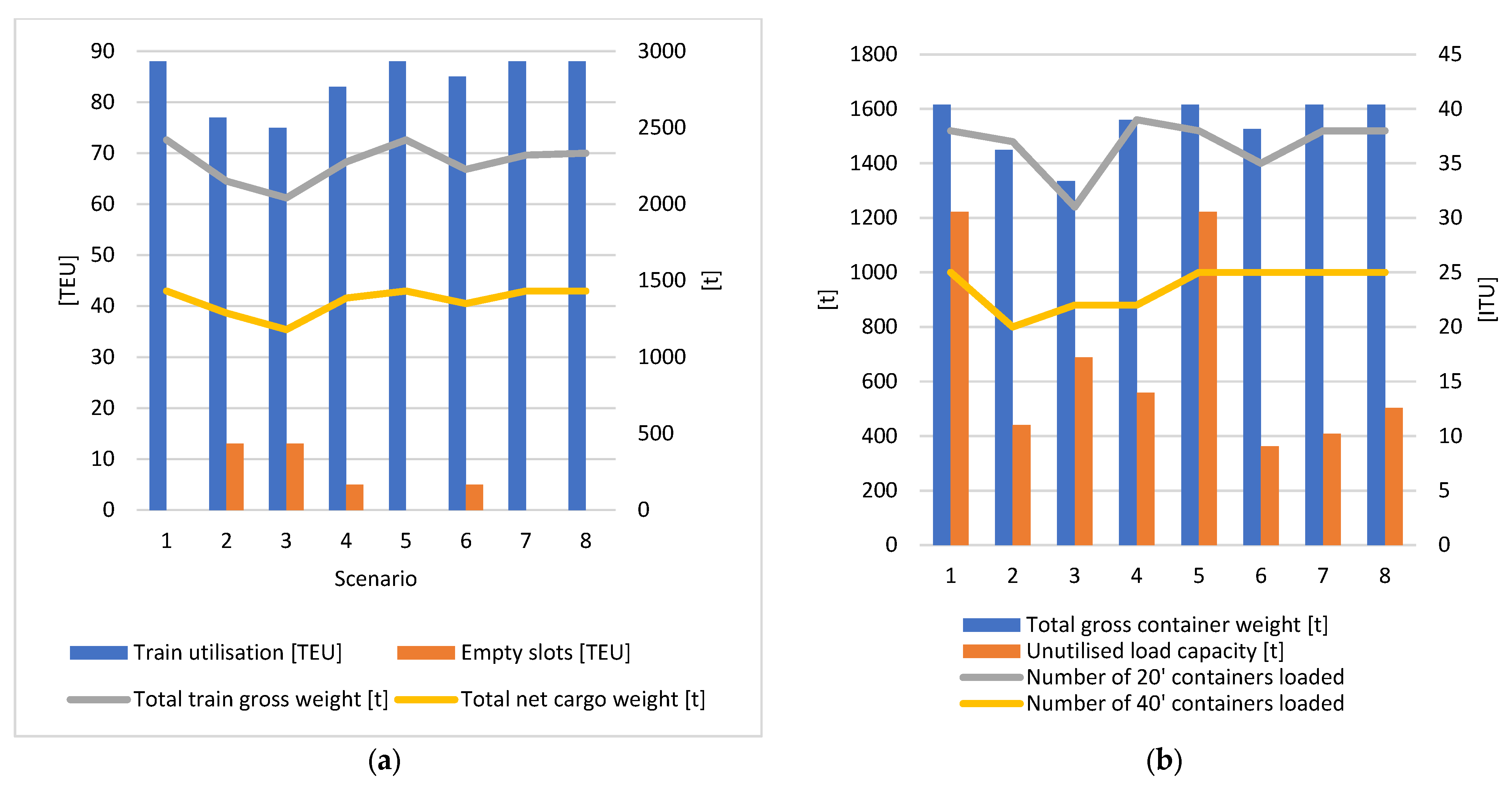
To better understand these differences, the analysis also covered the number of TEUs transported per train, the gross mass of transported containers, unused capacity (empty slots), and the number of containers carried, broken down into 20- and 40-foot ITUs (see Figure 5).
In the above figures, the number of transported TEUs ranged from 75 to 88, depending on the scenario. The lowest value was recorded in Scenario 3 (75 TEUs), while the highest occurred in Scenarios 1, 5, 7, and 8 (88 TEUs); in these cases, all loading slots were utilised. The highest number of empty slots was observed in Scenarios 2 and 3 (13 TEUs).
The gross train mass across all scenarios ranged from 2040 to 2419 t. The lowest value was recorded in Scenario 3 (2040 t), while the highest occurred in Scenarios 1 and 5 (2419 t). The net cargo mass, excluding container tare weight, ranged from 1179 to 1432 t. The smallest value was obtained in Scenario 3 (1179 t), and the highest in Scenarios 1, 5, 7, and 8 (1432 t).
The gross mass of the loaded containers ranged from 1335 to 1615 t across all scenarios. The lowest value was obtained in Scenario 3 (1335 t), while the highest occurred in Scenarios 1 and 5 (1615 t). Each train carried between 53 and 63 ITUs. The smallest number of 20-foot containers was recorded in Scenario 3 (31 units), and the largest in Scenario 4 (39 units). Conversely, the smallest number of 40-foot containers was observed in Scenario 2 (20 units), and the largest in Scenarios 1, 5, 6, 7, and 8 (25 units).
The unused payload capacity, expressed in tonnes, ranged from 363 to 1223 t. The lowest value was found in Scenario 6 (363 t, corresponding to 81% utilisation), while the highest occurred in Scenarios 1 and 5 (1223 t, corresponding to 57% utilisation).

4.2. Sensitivity Analysis

As part of the sensitivity analysis, the impact of extending the length of wagon consists from 600 m to 730 m on the characteristics discussed in the previous subsection was examined.
The scenarios involving 730 m wagon consists are described in Table A2 in Appendix A. As the main difference between these scenarios lies in the extended train length, they were designated as follows:
v —scenario number defined on the basis of the reference scenario.
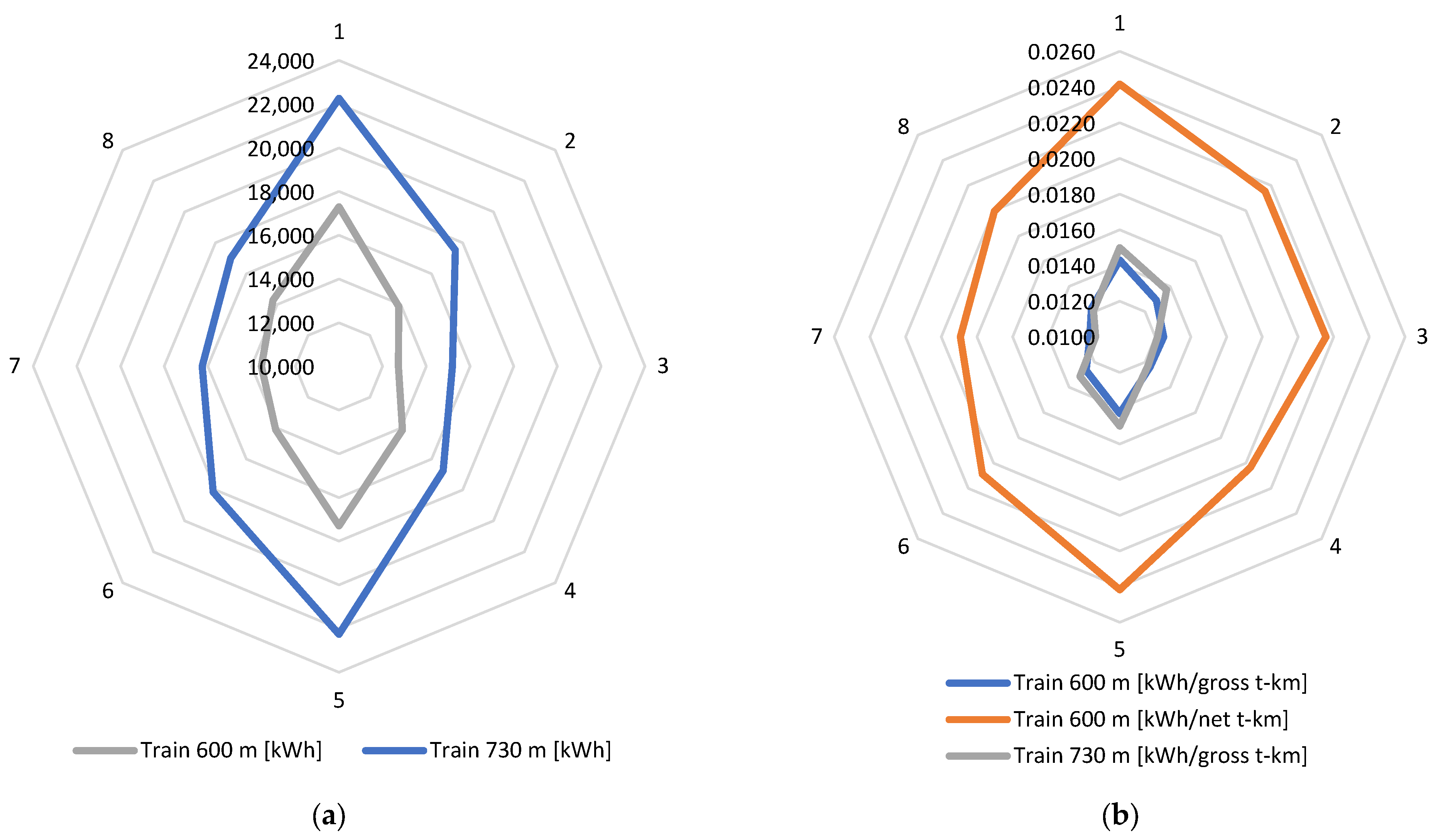
A comparison was made of total and specific electricity consumption, expressed in kWh/gross tkm and kWh/net tkm, for the given route (see Figure 6).
Based on the figures above, total energy consumption increased across all scenarios by an average of approximately 24%, ranging from 19% to 29% (from 12.7–17.3 MWh to 15.3–22.2 MWh). Energy consumption expressed in kWh/gross tkm and kWh/net tkm varied by scenario, showing both increases and decreases. It increased for scenarios v = 1, 2, 5, and 6 compared with their baseline counterparts, v = 1, 2, 5, and 6, by an average of 3.6–5.1%, while it decreased for scenarios v = 3, 4, 7, and 8 relative to v = 3, 4, 7, and 8 by an average of 2.1–3.3%.
In scenarios with a permissible axle load of 22.5 t/axle, energy consumption expressed in kWh/gross tkm and kWh/net tkm was on average 2–12% lower than in the scenarios with a 20 t/axle load. The lowest unit energy consumption was obtained in scenarios using 80-foot wagons with a 22.5 t/axle load. It amounted to 0.012 kWh/gross tkm and 0.019 kWh/net tkm for 600 m trains and 0.011 kWh/gross tkm and 0.018 kWh/net tkm for 730 m trains. The highest values were recorded in scenarios using 40-foot wagons, reaching 0.014 kWh/gross tkm and 0.024 kWh/net tkm for 600 m trains and 0.015 kWh/gross tkm and 0.025 kWh/net tkm for 730 m trains.
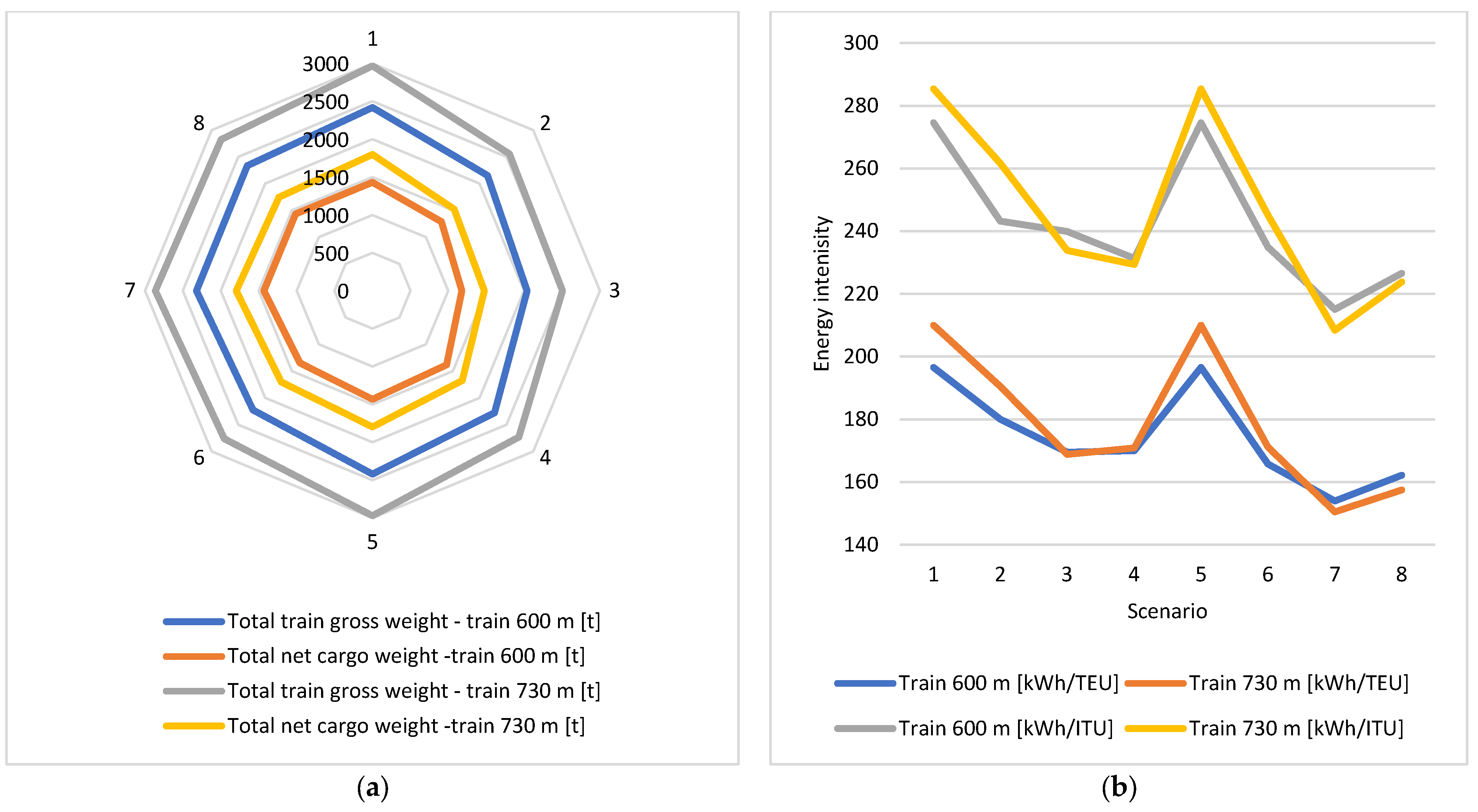
In the final stage of the sensitivity analysis, the impact of extending the train consist on increases in gross train mass and net cargo mass was examined, together with a comparison of unit energy consumption expressed in kWh/TEU and kWh/ITU (see Figure 7).
The first figure above indicates that both gross train mass and net cargo mass increased by an average of 21–23% in the scenarios with 730 m trainsets. Gross train mass rose from 2040–2419 t to 2507–2969 t, while net cargo mass increased from 1350–1432 t to 1476–1799 t. The second figure shows that unit energy consumption, expressed in kWh/TEU and kWh/ITU, was on average 3.21–6.82% higher in scenarios v = 1, 2, 5, and 6 compared with scenarios v = 1, 2, 5, and 6 and 0.41–2.9% lower in scenarios v = 3, 4, 7, and 8 compared with scenarios v = 3, 4, 7, and 8. The average energy consumption for 600 m trains amounted to 174 kWh/TEU and 242 kWh/ITU, while for 730 m trainsets the corresponding values were 178 kWh/TEU and 246 kWh/ITU. In scenarios with a permissible axle load of 22.5 t/axle, energy consumption expressed in kWh/TEU and kWh/ITU was on average 9–12 kWh lower than in scenarios with a 20 t/axle load for both 600 m and 730 m trains. The lowest unit energy consumption was observed in scenarios using 80-foot wagons with a 22.5 t/axle load, amounting to 153 kWh/TEU and 208 kWh/ITU for 730 m trains and 153 kWh/TEU and 215 kWh/ITU for 600 m trains. The highest values were recorded in scenarios using 40-foot wagons, reaching 209 kWh/TEU and 285 kWh/ITU for 730 m trains and 196 kWh/TEU and 274 kWh/ITU for 600 m trains.

5. Discussion

Based on the conducted research and supported by empirical evidence, the following conclusions have been formulated:
  • Energy consumption across all analysed scenarios ranged from 0.012 to 0.017 kWh/gross tkm and from 0.018 to 0.025 kWh/net tkm. Comparable values for energy consumption expressed in kWh/gross tkm have been reported in [61,63,64,65]. In [63,66], energy consumption for intermodal trains is reported at 0.0212 kWh per gross tonne-kilometre. For bulk trains, it is estimated at the same level, while for other train types it ranges from 0.0189 to 0.0327 kWh per gross tonne-kilometre, with higher values corresponding to speeds exceeding 130 km/h. The EcoTransIT [67] project provides estimates of energy use for freight trains based on total train weight. According to these findings, a train weighing 500 tonnes consumes about 0.024 kWh per gross tonne-kilometre, while a 1000-tonne train consumes approximately 0.017 kWh per gross tonne-kilometre and a 1500-tonne train requires around 0.014 kWh per gross tonne-kilometre. Bäckström [68] analysed data from an intermodal transport operator and estimated energy consumption at 5.84 kWh per train-kilometre, with an additional 0.0147 kWh per gross tonne-kilometre. In [64], figures illustrate specific energy consumption as a function of train gross mass. For trains below 500 tonnes, consumption exceeds 0.04 kWh/tkm. For trains of 1000 tonnes, it is approximately 0.02 kWh/tkm, consistent with [59], while for trains exceeding 2000 tonnes it is slightly above 0.01 kWh/tkm. Slightly higher values are reported in [61], where for 500-tonne trains specific energy consumption is estimated at 0.043–0.064 kWh/tkm, for 1000-tonne trains at 0.028–0.042 kWh/tkm, and for 2000-tonne trains at 0.018–0.027 kWh/tkm. Significantly higher values are reported in studies such as [69,70]. In [69], energy consumption for freight trains operating on an electrified network is estimated at 0.8–1.8 kWh/tkm. Another study [70] reports typical values in the range of 0.04–0.05 kWh/tkm, while noting that, depending on operating conditions, consumption may decrease to as low as 0.01–0.03 kWh/tkm.
  • Energy consumption values reported in the literature inevitably differ. This variation arises from differences in freight train operating parameters. The main factors include gross train mass, number of wagon axles, distance travelled, average speed, number of stops, rolling and aerodynamic resistance coefficients, the locomotive’s frontal area, and track gradient.
  • The validation of this study was also carried out using an empirical approach. For this purpose, data for 2024 were collected on the annual electricity consumption of all freight trains operating across the entire Polish railway network, as well as on transport performance. Energy consumption was expressed in MWh, while transport performance was measured in million tonne-kilometres. From the total transport performance, the share performed by diesel traction was excluded so that the analysis covered only operations carried out by electric vehicles. The total electricity consumption was then related to the adjusted transport performance. As a result of these calculations, the average energy consumption across the entire network in 2024 was estimated at 0.02503 kWh per net tonne-kilometre. This value corresponds to the upper bound of the results obtained in the present case study, thereby confirming their reliability. Additionally, analogous analyses were conducted for different types of bulk freight trains. In these cases, the average energy consumption values were also similar to those calculated for intermodal trains. The observed consistency indicates that the values presented in this study are representative and can be reliably used in further research and publications, both for bulk freight and intermodal transport. It is important to distinguish between energy consumption per gross train t-km and per net t-km. In many publications, the notion of unit energy consumption is not clearly defined. As noted earlier, the use of fixed energy consumption values introduces error, as demonstrated by the results of this case study. These values can vary substantially depending on the input parameters. To ensure comparability, it is therefore advisable to report the full set of train parameters for the case under consideration.
  • Although 40-foot wagons have favourable loading characteristics, allowing very high cargo mass without exceeding permissible bogie-axle loads, their operation is associated with relatively high energy use when launching an intermodal service. This is due to their having the greatest total tare mass among all wagon types. In addition, the higher number of bogie axles increases rolling resistance at the wheel–rail interface, which further raises energy consumption. Extending the train consist from 600 to 730 m does not reduce unit energy use; on the contrary, it increases it. In homogeneous consists of 40-foot wagons, the number of empty slots is practically negligible, as the four axles are positioned relatively close together, preventing axle overloading and enabling full utilisation of loading positions. Such consists can also carry the largest net cargo mass. However, the operational advantage of this wagon type diminishes relative to 60- and 80-foot wagons when the permissible axle load increases from 20 to 22.5 t.
  • Wagon consists composed of 60-foot wagons ranked second in terms of energy consumption (kWh/net tkm). In this case, energy use was driven primarily by the relatively low utilisation of available loading space, as the locomotive’s energy over a given route was distributed across a smaller cargo mass. The use of 60-foot wagons is disadvantageous from a space-utilisation perspective: at 20 t/axle, it is not possible to load three heavy 20-foot containers or one heavy 40-foot container together with a 20-foot container. This limitation becomes more pronounced when there is an insufficient number of ITUs of both types in the yard. For example, loading 30 sixty-foot wagons requires at least 30 forty-foot and 30 twenty-foot containers; otherwise, empty slots are likely to occur. It was also observed that 60-foot wagons are suitable when heavy 20-foot containers must be transported but 40-foot wagons are unavailable. The payload utilisation rate, measured in tonnes, ranged from approximately 75% to 77%. Furthermore, 60-foot wagons become a more attractive option once the permissible axle load increases from 20 to 22.5 t.
  • Train consists composed of 80-foot wagons exhibited some of the lowest energy-use levels, expressed in kWh/net tkm, kWh/gross tkm, kWh/TEU, and kWh/ITU. When consist length increased from 600 to 730 m, unit energy consumption continued to decline, unlike in trains composed of 60- and 40-foot wagons, although the differences were marginal. This may be attributed to slightly lower aerodynamic drag resulting from a smaller number of wagons, as fewer 80-foot wagons are required to form a train. However, the simulation showed that when a large number of heavy 20-foot containers are present in the yard and trains operate on lines limited to 20 t/axle, a significant number of empty slots occur in the consist. When the permissible axle load increases to 22.5 t/axle, the loading performance of 80-foot wagons improves considerably.
  • Using mixed consists appears particularly effective when heavy 20-foot containers must be transported but an insufficient number of 40-foot wagons are available. In such cases, the heaviest 40-foot containers are first loaded onto 80-foot wagons, the heaviest 20-foot containers are placed on 40-foot wagons, and the lightest 20- and 40-foot containers are allocated to 60-foot platforms. Simulation studies confirm these findings: mixed consists exhibit some of the lowest energy consumption levels, along with optimal utilisation of loading slots and payload capacity (in tonnes) under 20 t/axle scenarios. Combining different wagon types can therefore increase train utilisation and improve the energy efficiency of transport operations.
  • Operating 730-metre trains makes it possible to transport a significantly higher number of TEUs and ITUs. Consequently, such consists carry proportionally more cargo than 600-metre wagon consists. However, energy consumption does not consistently decrease across all scenarios; in most cases, the results are comparable to those obtained for the 600-metre configurations.
  • Increasing the permissible axle load from 20 to 22.5 t has a notably positive effect on train utilisation and energy efficiency. Across all key performance indicators, improvements of approximately 5–15% were observed.
  • It is not possible to unequivocally determine which wagon type is the most economically efficient in operation, as this depends on the parameters of the railway line on which the trains operate. From the perspective of energy consumption, 80-foot wagons perform best; however, at an axle-load limit of 20 t/axle, they may result in a large number of unused slots, in contrast to 40-foot wagons.
Despite its comprehensive nature, the proposed algorithm has certain limitations, namely:
  • The model is not suitable for estimating the energy use of refrigerated containers powered by onboard batteries or generator sets. In such cases, it would need to be extended with additional parameters, for example, differentiated rates for this type of intermodal transport unit, which is more expensive to move. A similar limitation applies to RO-RO intermodal transport: carrying semi-trailers, swap bodies, and road sets is significantly more energy-intensive than transporting containers and requires different wagon types, which may themselves consume energy.
  • In many regions—particularly the United States and Canada—double-stack trains are operated. For such trains, aerodynamic resistance coefficients must be adjusted to reflect the altered geometry and drag characteristics.
  • The model is limited to intermodal rail transport using electric locomotives. Many railway lines worldwide are not electrified. Its applicability to bulk rail transport is also limited; in such cases, the algorithm would require additional components and parameters.
  • The energy consumption model does not account for energy recuperation, that is, the recovery of braking energy.

6. Conclusions

The research showed that the use of different intermodal wagon types in non-uniform combinations has a significant impact on locomotive energy consumption.
The existing literature typically provides fixed values for energy consumption, which—as demonstrated in this study—constitutes a serious methodological limitation. The case study results indicate that energy use depends on numerous variables, including total train mass, speed, and route length. This study focused on three specific series of intermodal wagons; however, in practice there are several types of 40- and 60-foot wagons that differ in terms of payload, number of axles, overall length, and other characteristics. These differences have practical implications—for example, 40-foot wagons equipped with only two axles cannot carry two heavy 20-foot containers simultaneously. Further research should therefore include additional wagon types in order to broaden the analysis.
The findings shed new light on energy consumption in intermodal rail transport. In this study, energy use is closely correlated with parameters such as axle-load limits, train length, and wagon and container specifications, among others. These results open a new discussion on optimising intermodal transport from both economic and energy-efficiency perspectives. Until now, the influence of specific wagon types on energy use has not been systematically analysed. The conclusions presented here can therefore support logistics operators and rail carriers in improving the energy performance of their operations. This is particularly important in the context of growing global electricity demand and rising production costs. In Poland, energy costs already account for approximately 30% of the cost of operating a freight train. Lower energy consumption can therefore significantly reduce the total cost of freight transport on a given route.
The findings are also relevant for infrastructure design and management. In cost–benefit analyses conducted, for example, to secure EU funding for new rail infrastructure, it is necessary to demonstrate measurable environmental and energy benefits. The developed model enables precise simulation of energy consumption under defined infrastructure parameters. Given knowledge of a country’s energy mix, analysts can estimate greenhouse gas emissions based on train energy use. Assessing the impact of new infrastructure and transport operations is a fundamental requirement for obtaining EU funding for infrastructure development, such as railway lines and intermodal terminals, as well as for the acquisition of freight rolling stock, including locomotives and wagons.
It is important to note that, when planning a new railway line for freight or mixed traffic, at least three alternative route alignments must be developed. By taking into account parameters such as curvature, gradients and cant, design speed, and train mass, it is possible to estimate the annual energy consumption of freight trains for each design scenario. Within a multi-criteria analysis of railway projects, energy consumption—and consequently greenhouse gas emissions—may, depending on the assigned weighting, determine the selection of the preferred investment option. From a practical perspective, the study indicates which routes may be more advantageous for freight trains in terms of energy consumption and operating costs. Routes with steeper gradients can be expected to be more energy-intensive. A reasonable approach would therefore be to assign heavier trains (e.g., >1600 t gross) to lines with lower gradients, while lighter trains could be routed along steeper sections. At the same time, certain types of intermodal wagons, due to their more favourable loading characteristics (e.g., 40-foot wagons), could be assigned to lines with lower technical parameters (e.g., 20 t/axle) in order to maximise transported container mass, while other wagon types could be operated on lines with higher technical standards. Such an approach would be optimal in terms of both energy consumption and operating costs.
Research shows that 80-foot wagons are the optimal solution in terms of energy efficiency. However, it should be noted that when the axle load is limited to 20 tonnes, so-called empty slots often occur, generating significant costs for the intermodal operator. Under such conditions, ordering a fleet of 40-foot wagons may be economically justified. These, however, lose their advantage when the permissible axle load increases to 22.5 tonnes. In this case, the problem of empty slots in 80-foot wagons disappears, and the specific energy consumption remains the lowest compared to other train configurations.

Author Contributions

Conceptualisation, M.B., methodology, M.B., formal analyses, M.B., data curation, M.B., original draft preparation M.B. and J.A., visualisation M.B., project administration D.P., supervision D.P. and J.A., writing—review and editing D.P. and J.A., funding acquisition, D.P. and J.A. All authors have read and agreed to the published version of the manuscript.

Funding

This research has not external funding.

Institutional Review Board Statement

Not applicable.

Informed Consent Statement

Not applicable.

Data Availability Statement

The original contributions presented in this study are included in the article. Further inquiries can be directed to the corresponding author.

Conflicts of Interest

The authors declare no conflicts of interest. The funders had no role in the design of the study; in the collection, analysis, or interpretation of data; in the writing of the manuscript; or in the decision to publish the results.

Abbreviations

The following abbreviations are used in this manuscript:
EUEuropean Union
ITUIntermodal Transport Unit
TEUTwenty-foot Equivalent Unit
TEN-TTrans-European Transport Network
AGTCEuropean Agreement on Important International Combined Transport Lines and Related Installations
RO-RORoll-on/roll-off system
TLPPTrain Load Planning Problem
MEETMethodologies for Estimating Emissions from Transport
ARTEMISAssessment and Reliability of Transport Emission Models and Inventory Systems
ETWEcoTransIT World
kWh/tkmkWh/tonne-kilometre
z Wagon type
Y z 1 Diagnostic variable denoting the tare weight of a wagon of type z, in tones
Y z 2 Diagnostic variable denoting the payload capacity of a wagon of type z, in tones
Y z 3 Diagnostic variable denoting the capacity of a wagon of type z, in TEU
Y z 4 Diagnostic variable denoting the length of a wagon of type z, in metres
f Railway line class
a Container type
ϑ a Container size of type a , in TEU
m a Gross mass of a container of type a , in tones
L H T Wagon consist length, in metres
v Loading scenario number
i Number of containers
M t l ( v ) Gross mass of the train in the v - t h scenario, in tones
M g o o d s g r o s s ( v ) Gross mass of cargo in the v - t h scenario, in tones
M l o c Locomotive mass, in tones
M w a g ( v ) Mass of wagons in the v - t h scenario, in tones
M g o o d s n e t ( v ) Net mass of cargo in the v - t h scenario, in tones
p r Loading priority expressed as the number of days until loading
m i , a Gross mass of the i - t h container of type a, in tones
R j t z Load on the j t - t h bogie of a wagon of type z
α p e r f Permissible axle load in railway line class f , in tones per axle
T j t z Portion of the tare mass of a wagon of type z, in tones
c z Axle spacing in a wagon of type z, in metres
b i , a z Distance of the centre of gravity of the i - t h container of type a from the support centre ( R j t z ) of a wagon of type z, in meters
P L C Total wagon payload capacity, in tonnes
L G H Total wagon capacity, in TEU
w z Number of wagons of type z
W M a x z Maximum number of wagons of type z
V Set of loading scenarios
x i , k A binary decision variable equal to 1 if container i is assigned to wagon k and 0 otherwise (this variable determines whether the mass of the container is included in the load of wagon k )
U T ( v ) Utilisation of the loading space within the wagon consist in the v - t h scenario
m i , a t a r e Tare mass of the i - t h container of type a selected for loading, in tones
E S ( v ) Number of empty slots in the train consist in the v - t h scenario, in TEU
E T T W n t ( v ) Total energy consumption of the intermodal train in the v - t h scenario, calculated by the n t - t h method, in kWh
ϵ l o c Locomotive motor efficiency
E 4 ( v ) Energy required to overcome running resistance in the v - t h scenario, in kWh
p A U X ( v ) Power of auxiliary devices in the v - t h scenario, in kW
p A ( v ) Power required to overcome aerodynamic resistance in the v - t h scenario, in kW
p T ( v ) Power required to overcome rolling resistance in the v - t h scenario, in kW
p G ( v ) Power required to overcome gradient resistance in the v - t h scenario, in kW
d Distance travelled by the train, in kilometres
V a v g Average train speed in the v - t h scenario, in km/h
n s Number of train stops per 100 km
W t r ( v ) Energy required for train acceleration, in kWh
F J g r o s s ( v ) Energy use per gross train tone-kilometre of cargo, in kWh/gross-tkm
F J n e t ( v ) Energy use per net cargo tone-kilometre of cargo, in kWh/net-tkm
F J T E U ( v ) Energy use per TEU, in kWh/TEU
F J I T U ( v ) Energy use per ITU, in kWh/ITU

Appendix A

Table A1. Mass of the containers and their type.
Cont.No. ( i ) Cont. Type ( a ) Cont. Weight ( m i , a ) Priority ( p r ) Cont.No. ( i ) Cont. Type ( a ) Cont. Weight ( m i , a ) Priority ( p r )
1125.6142127.53
2129.2143128.53
3122.3144123.03
4122.5145123.13
5125.3146128.23
6126.4147123.73
7129.9148122.33
8122.0149129.93
9124.0150129.63
10122.7151125.13
11224.6152125.93
12224.4153125.53
13224.9154124.23
14229.0155128.93
15223.3156226.43
16228.1157224.33
17224.3158229.23
18229.4159227.53
19224.8160222.93
20124.7261229.83
21126.0262227.63
22129.0263223.53
23123.6264129.74
24128.5265127.64
25126.7266126.94
26127.2267125.24
27122.7268125.54
28123.7269123.44
29129.6270125.64
30126.0271128.64
31125.5272126.14
32125.7273128.44
33123.1274128.24
34224.1275129.14
35223.3276225.34
36223.6277227.04
37229.6278228.94
38222.7279229.04
39223.7280228.24
40222.9281228.04
41224.2282229.94
Table A2. Characteristics of the wagon sets (600 m and 730 m trains).
ScenarioNo. ( v ) Max. Lengths of Wagon Consists [m]Permissible Axle Load ( α p e r f )  [t/axle]Type of Wagon FleetEmpty Wagon Set Weight [t]Max. Capacity [t]Max. Capacity [TEU]Wagon Set Length [m]
16002044 × 40′704283888599.72
26002030 × 60′600189090589.2
36002022 × 80′605202488596.2
4600207 × 40′ + 6 × 60′ + 14 × 80′617211788592.65
560022.544 × 40′704283888599.72
660022.530 × 60′600189090589.2
760022.522 × 80′605202488596.2
860022.57 × 40′ + 6 × 60′ + 14 × 80′617211788592.65
1′7302053 × 40′8483419106722.39
2′7302037 × 60′7402331111726.68
3′7302027 × 80′7432484108731.7
4′730207 × 40′ + 14 × 60′ + 13 × 80′749.52529108722.7
5′73022.553 × 40′8483418106722.4
6′73022.537 × 60′7402331111726.7
7′73022.527 × 80′7432484108731.7
8′73022.57 × 40′ + 14 × 60′ + 13 × 80′749.52529108722.7
Table A3. Results for the subsequent scenarios (600 m and 730 m trains).
ScenarioNo. ( v ) Total Gross Container Weight [t]Unutilised Load Capacity [t]Number of 20′ Containers LoadedNumber of 40′ Containers LoadedSum ofITUsLoad Capacity Utilisation Rate [%]ScenarioNo.Total Train Gross Weight [t]Total Net Cargo Weight [t]
11615122338256357%124191432
2144944137205777%221491288
3133568931225366%320401179
4156055839226174%422771386
51615122338256357%524191432
6152736335256081%622271350
7161540938256380%723201432
8161550238256376%823321432
1′2021139850287859%1′29691799
2′171561642256774%2′25551523
3′166482040256567%3′25071476
4′188264748257374%4′27321677
5′2021139850287859%5′29691799
6′192240942327482%6′27621701
7′202146348307881%7′28641795
8′197055944327678%8′28201745

References

  1. Jacyna, M.; Pyza, D.; Jachimowski, R. Transport Intermodalny—Projektowanie Terminali Intermodalnych; PWN: Warszawa, Poland, 2017. [Google Scholar]
  2. Brzeziński, M. Method of Locating Intermodal Terminals for the Sustainable Development of Poland. Ph.D. Thesis, Division of Traffic Control and Transport Infrastructure, Warsaw University of Technology, Warsaw, Poland, 2024. [Google Scholar]
  3. Archutowska, J. (Ed.) White Book on Railway Development, 2nd Updated ed.; Available online: https://www.cpk.pl/en/the-white-book-on-railway-development (accessed on 1 August 2025).
  4. Regulation (EU) 2024/1679 of the European Parliament and of the Council of 13 June 2024 on Union Guidelines for the Development of the Trans-European Transport Network, Amending Regulations (EU) 2021/1153 and (EU) No 913/2010 and Repealing Regulation (EU) No 1315/2013. Available online: https://publications.europa.eu/resource/cellar/cc3395a5-3516-11ef-b441-01aa75ed71a1.0006.03/DOC_1 (accessed on 1 September 2025).
  5. Kowalski, S. Obtaining EU Funding for the Development of Intermodal Transport in Poland. Logist. Transp. 2013, 20, 21–28. [Google Scholar]
  6. UIC 2024 Report on Combined Transport in Europe. Available online: https://uic.org/IMG/pdf/uic_uirr_report_2024-2.pdf (accessed on 1 September 2025).
  7. Brzeziński, M.; Pyza, D. A Refined Model for Carbon Footprint Estimation in Electric Railway Transport. Energies 2023, 16, 6567. [Google Scholar] [CrossRef] [Scilit]
  8. Bulakh, M. Evaluation and Reduction of Energy Consumption of Railway Train Movement on a Straight Track Section with Reduced Freight Wagon Mass. Energies 2025, 18, 280. [Google Scholar] [CrossRef] [Scilit]
  9. Qi, T.; Mei, M. Analysis on Energy Efficiency and Rapidity of High-Speed Train Operation. In Proceedings of the 2022 3rd Asia-Pacific Conference on Image Processing, Electronics and Computers; ACM: Dalian, China, 2022; pp. 643–651. [Google Scholar]
  10. Janić, M. Estimation of Direct Energy Consumption and CO2 Emission by High Speed Rail, Transrapid Maglev and Hyperloop Passenger Transport Systems. Int. J. Sustain. Transp. 2021, 15, 696–717. [Google Scholar] [CrossRef] [Scilit]
  11. Nehring, K.; Kiszkowiak, Ł. Improving Aerodynamic Performance of Intermodal Trains through Optimisation of Loading Plans. Arch. Transp. 2025, 76, 137–159. [Google Scholar] [CrossRef] [Scilit]
  12. Heinold, A. Comparing Emission Estimation Models for Rail Freight Transportation. Transp. Res. Part D Transp. Environ. 2020, 86, 102468. [Google Scholar] [CrossRef] [Scilit]
  13. Yuan, M.; Thellufsen, J.Z.; Lund, H.; Liang, Y. The Electrification of Transportation in Energy Transition. Energy 2021, 236, 121564. [Google Scholar] [CrossRef] [Scilit]
  14. Jarnut, M.; Kaniewski, J.; Buciakowski, M. Energy Storage Systems for Fluctuating Energy Sources and Fluctuating Loads—Analysis of Selected Cases. Energies 2025, 18, 4792. [Google Scholar] [CrossRef] [Scilit]
  15. Serrano-Arévalo, T.I.; Ochoa-Barragán, R.; Ramírez-Márquez, C.; El-Halwagi, M.; Abdel Jabbar, N.; Ponce-Ortega, J.M. Energy Storage: From Fundamental Principles to Industrial Applications. Processes 2025, 13, 1853. [Google Scholar] [CrossRef] [Scilit]
  16. Khan, Z.A.; Ullah, A.; Ul Haq, I.; Hamdy, M.; Maria Mauro, G.; Muhammad, K.; Hijji, M.; Baik, S.W. Efficient Short-Term Electricity Load Forecasting for Effective Energy Management. Sustain. Energy Technol. Assess. 2022, 53, 102337. [Google Scholar] [CrossRef] [Scilit]
  17. Kuzior, A.; Staszek, M. Energy Management in the Railway Industry: A Case Study of Rail Freight Carrier in Poland. Energies 2021, 14, 6875. [Google Scholar] [CrossRef] [Scilit]
  18. Melnyk, O.; Onishchenko, O.; Onyshchenko, S.; Golikov, V.; Sapiha, V.; Shcherbina, O.; Andrievska, V. Study of Environmental Efficiency of Ship Operation in Terms of Freight Transportation Effectiveness Provision. TransNav Int. J. Mar. Navig. Saf. Sea Transp. 2022, 16, 723–729. [Google Scholar] [CrossRef] [Scilit]
  19. Zhang, D.; Zhou, F.-R.; Tang, Y.-Y.; Tao, Z.-Y.; Peng, Q.-Y. Optimization of the Loading Plan for a Railway Wagon from the Perspectives of Running Safety and Energy Conservation. Energy 2023, 280, 128229. [Google Scholar] [CrossRef] [Scilit]
  20. IEA World Energy Outlook. 2025. Available online: https://iea.blob.core.windows.net/assets/1438d3a5-65ca-4a8a-9a41-48b14f2ca7ea/WorldEnergyOutlook2025.pdf (accessed on 1 December 2025).
  21. IEA. Electricity 2025 Analysis and Forecast to 2027; IEA: Paris, France, 2025. [Google Scholar]
  22. DNV. Energy Transition Outlook: A Global and Regional Energy Forecast to 2060; DNV: Høvik, Norway, 2025. [Google Scholar]
  23. IRENA. World Energy Transitions Outlook 2024: 1.5 °C Pathway; IRENA: Abu Dhabi, United Arab Emirates, 2024. [Google Scholar]
  24. GSR Global Status Report 2025: A Comprehensive Annual Overview of the State of Renewable Energy. Available online: https://www.ren21.net/gsr-2025/ (accessed on 3 December 2025).
  25. Pulido-Sánchez, D.; Capellán-Pérez, I.; Castro, C.d.; Frechoso, F. Material and Energy Requirements of Transport Electrification. Energy Environ. Sci. 2022, 15, 4872–4910. [Google Scholar] [CrossRef] [Scilit]
  26. BP Energy Outlook. Available online: https://www.bp.com/content/dam/bp/business-sites/en/global/corporate/pdfs/energy-economics/energy-outlook/bp-energy-outlook-2025.pdf (accessed on 12 February 2026).
  27. Raźniewska, M.; Wronka, A. Transport Fleet Electrification Development Conditions—Perspective of Transport, Shipping, and Logistics Industry in Poland. Energies 2024, 17, 4288. [Google Scholar] [CrossRef] [Scilit]
  28. UIC Activity Report 2019. Available online: https://uic.org/IMG/pdf/uic_activity_report_2019.pdf (accessed on 15 January 2026).
  29. UIC Activity Report 2024. Available online: https://uic.org/IMG/pdf/uic_activity_report_2024.pdf (accessed on 30 January 2026).
  30. EY European Economic Outlook What Will the Tariffs Bring? Available online: https://www.ey.com/content/dam/ey-unified-site/ey-com/en-pl/insights/economic-analysis-team/documents/ey-european-economic_outlook-may25.pdf (accessed on 13 February 2026).
  31. Ćwil, M.; Bartnik, W.; Jarzębowski, S. Railway Vehicle Energy Efficiency as a Key Factor in Creating Sustainable Transportation Systems. Energies 2021, 14, 5211. [Google Scholar] [CrossRef] [Scilit]
  32. Gołębiowski, P.; Jacyna, M.; Stańczak, A. The Assessment of Energy Efficiency versus Planning of Rail Freight Traffic: A Case Study on the Example of Poland. Energies 2021, 14, 5629. [Google Scholar] [CrossRef] [Scilit]
  33. Kostrzewski, A.; Nader, M.; Kostrzewski, M. Racjonalizacja Rozłożenia Wybranych Jednostek Transportu Intermodalnego Na Długości Ładunkowej Pociągu. Pr. Nauk. Politech. Warsz. 2018, 120, 201–208. [Google Scholar]
  34. Kłodawski, M.; Nehring, K.; Jachimowski, R.; Lipińska, J. The Impact of the Intermodal Terminal Operation Strategy on Container Train Loading Duration. Transp. Probl. 2024, 19, 163–176. [Google Scholar] [CrossRef] [Scilit]
  35. Siri, S.; Palmiere, A.; Ambrosino, D. Multi-Objective Optimization Methods for Train Load Planning in Seaport Container Terminals. IEEE Trans. Autom. Sci. Eng. 2024, 21, 3216–3228. [Google Scholar] [CrossRef] [Scilit]
  36. Nehring, K.; Kłodawski, M.; Jachimowski, R.; Klimek, P.; Vasek, R. Simulation Analysis of the Impact of Container Wagon Pin Configuration on the Train Loading Time in the Intermodal Terminal. Arch. Transp. 2021, 60, 155–169. [Google Scholar] [CrossRef] [Scilit]
  37. Mantovani, S.; Morganti, G.; Umang, N.; Crainic, T.G.; Frejinger, E.; Larsen, E. The Load Planning Problem for Double-Stack Intermodal Trains. Eur. J. Oper. Res. 2018, 267, 107–119. [Google Scholar] [CrossRef] [Scilit]
  38. Foti, L.; Maratea, M.; Sacone, S.; Siri, S. Solving Train Load Planning Problems with Boolean Optimization. In Proceedings of the 19th RCRA International Workshop on Experimental Evaluation of Algorithms for Solving Problems with Combinatorial Explosion, Rome, Italy, 14–16 June 2012. [Google Scholar]
  39. Ambrosino, D.; Caballini, C. New Solution Approaches for the Train Load Planning Problem. EURO J. Transp. Logist. 2019, 8, 299–325. [Google Scholar] [CrossRef] [Scilit]
  40. Corry, P.; Kozan, E. Optimised Loading Patterns for Intermodal Trains. Spectr. 2007, 30, 721–750. [Google Scholar] [CrossRef] [Scilit]
  41. Bruns, F.; Goerigk, M.; Knust, S.; Schöbel, A. Robust Load Planning of Trains in Intermodal Transportation. Spectr. 2014, 36, 631–668. [Google Scholar] [CrossRef] [Scilit]
  42. Anghinolfi, D.; Paolucci, M. A General Purpose Lagrangian Heuristic Applied to the Train Loading Problem. Procedia—Soc. Behav. Sci. 2014, 108, 37–46. [Google Scholar] [CrossRef] [Scilit]
  43. Wymiary i Ładowność 20-Stopowych i 40-Stopowych Kontenerów Standardowych|DSV. Available online: https://www.dsv.com/pl-pl/nasze-rozwiazania/rodzaje-transportu/fracht-morski/wymiary-kontenerow-morskich/kontener-standardowy (accessed on 29 August 2025).
  44. Wardrop, A. MTRAIN User’s Manual; Version 89A; State Rail: New South Wales, Australia, 1989. [Google Scholar]
  45. Lee, C.K.; Sun, C.H. A Simulation Study on Energy Saving Effect of Train Operation. Transp. Plan. J. 2001, 30, 237–252. [Google Scholar] [CrossRef]
  46. Jong, J.-C. Models for Estimating Energy Consumption of Electric Trains. J. East. Asia Soc. Transp. Stud. 2005, 5, 278–291. [Google Scholar] [CrossRef]
  47. Parajuli, A. Modelling Road and Rail Freight Energy Consumption: A Comparative Study. Master’s Thesis, Queensland University of Technology, Brisbane, Australia, 2005. [Google Scholar]
  48. Lukaszewicz, P. Energy Consumption and Running Time for Trains: Modelling of Running Resistance and Driver Behaviour Based on Full Scale Testing; Royal Institute of Technology, Department of Vehicle Engineering: Stockholm, Sweden, 2001. [Google Scholar]
  49. Huo, X.-S.; Liu, T.-H.; Chen, Z.-W.; Li, W.-H.; Niu, J.-Q.; Gao, H.-R. Aerodynamic Characteristics of Double-Connected Train Groups Composed of Different Kinds of High-Speed Trains under Crosswinds: A Comparison Study. Alex. Eng. J. 2023, 64, 465–481. [Google Scholar] [CrossRef] [Scilit]
  50. Hickman, J.; Hassel, D.; Joumard, R.; Samaras, Z.; Sorenson, S. Methodology for Calculating Transport Emissions and Energy Consumption; Transport Research Laboratory: Washington, DC, USA, 1999. [Google Scholar]
  51. Lindgreen, E.B.G.; Sorenson, S.C. Simulation of Energy Consumption and Emissions from Rail Traffic; Department of Mechanical Engineering, Technical University of Denmark: Lyngby, Denmark, 2005. [Google Scholar]
  52. EcoTransIT. World Initiative Ecological Transport Information Tool for Worldwide Transports; EcoTransIT Word: Hannover, Germany, 2019. [Google Scholar]
  53. Kirschstein, T.; Meisel, F. GHG-Emission Models for Assessing the Eco-Friendliness of Road and Rail Freight Transports. Transp. Res. Part B Methodol. 2015, 73, 13–33. [Google Scholar] [CrossRef] [Scilit]
  54. Heinold, A.; Meisel, F. Emission Limits and Emission Allocation Schemes in Intermodal Freight Transportation. Transp. Res. Part E Logist. Transp. Rev. 2020, 141, 101963. [Google Scholar] [CrossRef] [Scilit]
  55. Heinold, A.; Meisel, F. Emission Rates of Intermodal Rail/Road and Road-Only Transportation in Europe: A Comprehensive Simulation Study. Transp. Res. Part Transp. Environ. 2018, 65, 421–437. [Google Scholar] [CrossRef] [Scilit]
  56. Favre, A. Rail Statistics on Energy Consumption and Emissions. Available online: https://unece.org/sites/default/files/2024-05/Rail%20statistics%20on%20energy%20consumption%20and%20emissions%20-%20UIC.pdf (accessed on 2 September 2025).
  57. Vleugel, J.M.; Bal, F. Climate Change and Resilient Rail Freight Transport. In Proceedings of the Sustainable Development and Planning, Online, 17 August 2022; pp. 79–88. [Google Scholar]
  58. Calculating GHG Emissions for Freight Forwarding and Logistics Services in Accordance with EN 16258—Terms, Methods, Examples. Available online: https://www.clecat.org/media/CLECAT_Guide_on_Calculating_GHG_emissions_for_freight_forwarding_and_logistics_services.pdf (accessed on 2 September 2025).
  59. Gallas, D.; Michalak, P.; Cichy, R. Analysis of Benefits and Drawbacks of Using Hybrid Drive Special Purpose Vehicles. Pojazdy Szyn. 2025, 1–2, 3–8. [Google Scholar] [CrossRef] [Scilit]
  60. PKP Cargo. Available online: https://www.pkpcargo.com/wp-content/uploads/2023/10/pkpcargo_katalogwagonow_3008_19.pdf (accessed on 1 March 2026).
  61. W 2021 Dalszy Wzrost Przewozów Intermodalnych w Polsce. Available online: https://utk.gov.pl/pl/aktualnosci/18679,W-2021-dalszy-wzrost-przewozow-intermodalnych-w-Polsce.html (accessed on 30 August 2025).
  62. Rozporządzenie Ministra Infrastruktury 1 z Dnia 31 Grudnia 2002 r. w Sprawie Warunków Technicznych Pojazdów Oraz Zakresu Ich Niezbędnego Wyposażenia. Available online: https://isap.sejm.gov.pl/isap.nsf/DocDetails.xsp?id=wdu20030320262 (accessed on 10 March 2026).
  63. Flodén, J. Rail Freight Costs—Some Basic Cost Estimates for Intermodal Transport; University of Gothenburg: Gothenburg, Sweden, 2011. [Google Scholar]
  64. Topsector Logistiek Insight into the Energy Consumption, CO2 Emissions and NOx Emissions of Rail Freight Transport. Available online: https://topsectorlogistiek.nl/wp-content/uploads/2018/04/20180318-Emissions-of-railtransport-Topsector-Logistics.pdf (accessed on 2 September 2025).
  65. Combined Transport Directive: Sustainable Means Combining Freight Transport Modes. Railway PRO 2024. Available online: https://www.railwaypro.com/wp/combined-transport-directive-sustainable-means-combining-freight-transport-modes/ (accessed on 10 March 2026).
  66. Trafikvert Swedish Transport AdministrationAnnual Report 2010. Available online: https://www.scribd.com/document/816447765/Trafikverket-Annual-Report-2010 (accessed on 22 March 2026).
  67. EcoTransIT: Ecological Transport Information Tool. Environmental Methodology and Data. Available online: https://www.hupac.com/downdoc.php?id_doc=185&lng=1&masterid=g1_5&rif=36170 (accessed on 1 September 2025).
  68. Bäckström, S.; Bohlin, M.; Franzen, U.; Jonsson, P. Miljökalkyler För Intermodala Transportkedjor Detaljerad Beräkningsmetodik Och Relevanta Schablonvärden; Rapp. Nr 20096; WSP Analys & Strategi, SIR-C Swedish Intermodal Transport Research Centre: Gothenburg, Swededn, 2009. [Google Scholar]
  69. García-Álvarez, A.; Pérez-Martínez, P.J.; González-Franco, I. Energy Consumption and Carbon Dioxide Emissions in Rail and Road Freight Transport in Spain: A Case Study of Car Carriers and Bulk Petrochemicals. J. Intell. Transp. Syst. 2013, 17, 233–244. [Google Scholar] [CrossRef] [Scilit]
  70. Gurrì, S.; Bocchieri, M.; Galasso, D.; Operti, V.; Dalla Chiara, B. Analisi Della Velocità di un Elettrotreno Merci a Potenza Distribuita su Linee ad Alta Velocità.|EBSCOhost. Available online: https://openurl.ebsco.com/contentitem/doi:10.57597%2FIF.05.2023.ART.1?sid=ebsco:plink:crawler&id=ebsco:doi:10.57597%2FIF.05.2023.ART.1 (accessed on 31 August 2025).
Figure 1. Loading instructions for 40′ and 60′ wagons. Source: [39].
Applsci 16 03567 g001
Figure 2. Research model.
Applsci 16 03567 g002
Figure 3. Example of the reaction forces for 4-axle wagons (a) and 6-axle wagons (b).
Applsci 16 03567 g003
Figure 4. Total and unit energy consumption.
Applsci 16 03567 g004
Figure 5. (a) Utilisation analysis. (b) Number of ITUs loaded and gross mass of the train.
Applsci 16 03567 g005
Figure 6. (a) Total energy consumption comparison for 600 and 730 m long wagon consists. (b) Unit energy consumption comparison for 600 and 730 m long wagon consists.
Applsci 16 03567 g006
Figure 7. (a) Total gross and net cargo weights for 600 and 730 m long wagon consists. (b) Unit energy consumption comparison for 600 and 730 m long wagon consists.
Applsci 16 03567 g007
Table 1. The designations used in the energy consumption measurement.
Method
MEETARTEMISETWMesoscopic
ParametersFirst approach:
Constants determined based on empirical observations ( B 0 , B 1 ) ; average velocity ( V a v g ) ; travelled distance ( d ) ; the maximal train payload ( M t l ) .
Second approach:
constants determined based on empirical observations ( G 0 , G 1 , G 2 ) ; number of stops ( n s ) ; maximal velocity of the route ( V m a x ) ; gravitation ( g ) ; trip altitude difference ( h ); travelled distance ( d ) ; the maximal train payload ( M t l ) .
Number of stops ( n s ) ; maximal velocity of the route ( V m a x ) ; gross train weight ( M t l ) ; mass of locomotive ( M l o c ) ; average velocity ( V a v g ) ; gravitation ( g ) ; trip altitude difference ( h ); travelled distance ( d ) ; air density ( ρ A ) ; locomotive front surface; number of stops per 100 km ( n s ) ; aerodynamic and rolling resistance factors of locomotives and wagons ( c l o c L A , c w a g A , c l o c R T , c w a g R T ) ; surface rolling resistance factors ( c 1 , c 2 ) ; number of axles in wagons of the z - t y p e ( n a x z ) ; number of the z - t y p e wagons ( w z ) ; train’s acceleration ( a p ) ;
the efficiency of the locomotive ( ϵ l o c ) .
Parameter related to the trip altitude difference ( q ) , train gross mass ( M t ) , train space utilisation rate ( c g ) ;wagons of the z - t y p e payload ( M P w z ) ; wagons of the z - t y p e max. payload ( M X w z ) ; empty travelled
distance ( d e m p t ) ; loaded travelled
distance ( d l o a d ) ; the efficiency of the locomotive ( ϵ l o c ) .
Number of stops ( n s ) ; maximal velocity of the route ( V m a x ) ; the maximal train payload ( M t l p ) ; mass of locomotive ( M l o c ) ; average velocity ( V a v g ) ; gravitation ( g ) ; trip altitude difference ( h ); travelled distance ( d ) ; air density ( ρ A ) ; locomotive front surface; number of stops per 100 km ( n s ) ; aerodynamic and rolling resistance factors of locomotives and wagons ( c l o c L A , c w a g A , c l o c R T , c w a g R T ) ; surface rolling resistance factors ( c 1 , c 2 ) ; number of axles in wagons of the z - t y p e   ( n a x z ) ; number of the z - t y p e wagons ( w z ) ; the efficiency of the locomotive ( ϵ l o c ) .
Source: Based on [7,53,54,55].
Table 2. Wagon diagnostic variables.
Type of Wagon
Diagnostic variable z = 1 z = 2 z = 3
Tare weight of the wagon ( Y z 1 [ t ] )162027.5
Payload capacity ( Y z 2 [ t ] )64.56392
Loading capacity ( Y z 3 [ T E U ] )234
Total length ( Y z 4 [ m ] )13.6319.6427.1
Source: Based on [60].
Table 3. Train and route parameters.
ParameterUnitValue
Locomotive weight ( M l o c ) t100
Trip’s altitude difference ( h ) m150
Locomotive efficiency ( ϵ l o c ) %90
Air density ( ρ A ) kg/m31.225
Locomotive front surface ( A ) m212.3
Gravitation ( g ) m/s29.81
Coefficients ( c l o c L A / c w a g A / c l o c R T / c w a g R T / c 1 / c 2 ) -1.1/0.22/0.004/0.0006/0.0005/0.0006
Power of auxiliary devices ( p A U X ) kW100
Distance ( d ) km500
Number of stops per 100 km ( n s ) -2
Average velocity ( V a v g ) km/h80
Number of wagon axles ( n a x z ) - z = 1 z = 2 z = 3
446
Source: Based on [7,51,54,55,60].
Table 4. Wagon parameters.
ParameterValue [m]
Axle spacing in the z -type wagon ( c 1,2 , 3 [ m ] ) 8.0/14.2/10.58
Portion of the wagon’s tare weight (symmetric) ( T j t 1,2 [ t ] ) 8.0/10.0
Portion of the wagon’s tare weight (asymmetric) ( T j t 3 [ t ] ) 8.8, 9.9 *, 8.9 )
Distance of the centre of gravity of the i - t h container of type a from the support point ( R j t z ) of the z-type wagon ( b i , a z [ m ] )
Configuration—40-foot wagon:
2 × 20-foot0.934/7.066
1 × 40-foot4.0
Configuration—60-foot wagon:
3 × 20-foot0.976/7.1/13.224
1 × 40-foot + 1 × 20-foot0.985/10.166
Configuration—80-foot wagon:
4 × 20-foot (wagon symmetry condition)3.535/9.635
2 × 20-foot + 1 × 40-foot (wagon symmetry condition)3.535/9.635/6.564
2 × 40-foot (wagon symmetry condition)6.564
Source: Based on [60]. * Value for the section of the wagon.
Disclaimer/Publisher’s Note: The statements, opinions and data contained in all publications are solely those of the individual author(s) and contributor(s) and not of MDPI and/or the editor(s). MDPI and/or the editor(s) disclaim responsibility for any injury to people or property resulting from any ideas, methods, instructions or products referred to in the content.