Estimating Economic Activity from Satellite Embeddings

Abstract

Earth Embedding (EMB) is a method that adapts embedding techniques from Large Language Models (LLMs) to compress the information contained in multiple remote sensing satellite images into feature vectors. This article introduces a new approach to measuring economic activity from EMBs. Using the Google Satellite Embedding Dataset (GSED), we extract a 64-dimensional representation of the Earth’s surface that integrates optical and radar imagery. A neural network maps these embeddings to nighttime light (NTL) intensity, yielding a 32-dimensional “income-aware” feature space aligned with economic variation. We then predict GDP levels and growth rates across countries and compare the results with those of traditional NTL-based models. The Earth-Embedding (EMB) based estimator achieves substantially lower mean squared error in estimating GDP levels. Combining the two sources yields the best overall accuracy. Further analysis shows that EMB performs particularly well in low-statistical-capacity and high-income economies. These results suggest that satellite embeddings can provide a scalable, globally consistent framework for monitoring economic development and validating official statistics.

1. Introduction

An accurate system of national accounts is essential for economic analysis. However, measurement error remains prevalent in national accounts data from developing countries. Devarajan [1] argues that limited statistical capacity and institutional constraints in low-income countries have produced persistent distortions in official data, which he characterizes as Africa’s “statistical tragedy.” These distortions become particularly evident during base-year adjustments. For example, GDP estimates for Ghana and Malawi increased sharply after methodological updates, which Young [2] cites as evidence of systematic measurement error in African growth statistics. Jerven [3] further shows that unon-synchronized revisions of methods and data sources have reduced temporal and cross-country comparability of GDP data in Sub-Saharan Africa. This issue is not unique to Africa. In Asia, there are also many debates about the statistical quality of emerging economies. Holz [4] reviews longstanding concerns about the quality of China’s GDP data and the institutional context of its compilation, while Subramanian [5] raises concerns about the accuracy of India’s GDP after the 2011 methodological revision. Overall, methodological changes and political incentives introduce nontrivial measurement error into official GDP data, which limits the reliability of national accounts for empirical analysis. This concern has motivated the use of alternative proxies for economic activity. Satellite data have become important tools for constructing economic proxies, particularly in situations where reliable official statistics are unavailable or delayed [6,7,8,9].

Nighttime lights were the first satellite products that researchers identified as useful for estimating economic indicators. Representative nighttime light systems include the Defense Meteorological Satellite Program–Operational Linescan System (DMSP–OLS) [10] and the Suomi National Polar-Orbiting Partnership–Visible Infrared Imaging Radiometer Suite (Suomi NPP–VIIRS) [11], as well as recently launched, higher-resolution platforms such as Luojia-1 [12] and SDGSAT-1 [13]. Nighttime light imagery directly captures illumination from infrastructure, transportation activity, and other indicators closely associated with economic activity. Therefore, it became the earliest and most extensively studied form of satellite data in economics.

As discussed before, GDP is not directly observed but inferred through imperfect statistical systems. Therefore, the estimation of national accounts data is a classic latent variable problem [14] in which official GDP data serve as noisy proxies for true economic output. The measurement error in official GDP can thus bias coefficient estimates and distort cross-country comparisons [15]. When the outcome of interest is a latent variable subject to classical measurement error, the optimal use of data involves combining multiple imperfect measures rather than relying on a single proxy [16]. This interpretation motivates approaches that combine official GDP data with independent signals, such as satellite nighttime lights, within a statistical framework to more accurately estimate latent economic output. Henderson et al. [6] developed such a framework. They applied the changes in nighttime lights data to augment official income growth measures and constructed optimal composite estimates of true economic growth, with weights determined by the relative reliability of the two signals. Hu et al. [17] developed a more general semi-parameter model to characterize the relationship between nighttime lights and GDP. Chen et al. [18] and Li et al. [19] explored how the dynamics of nighttime light can reflect economic growth and structural transformation within countries. Nighttime light data are also used for spatial pattern analysis related to economics. For example, Yan et al. [20] used nighttime light data combined with POI data to capture spatial patterns of China’s nighttime economy. Other economic-related indexes are also predicted based on nighttime light data, for example, Gao et al. [21] used nighttime light data to model electricity consumption in Cambodia. Another example is Yang et al. [22] who studied the relationship between nighttime light data and agriculture output value.

The capacity of national statistical systems plays a key role in cross-country GDP estimation as discussed by Henderson et al. [6] and Hu et al. [17]. By shaping the variance and bias of official GDP estimates while remaining independent of errors in remote-sensing measures, statistical capacity provides a natural source of heterogeneity for identifying the joint error structure across multiple proxies and improving inference on latent output. Dang et al. [23] introduces the Statistical Performance Indicators and Index (SPI) as a replacement for the earlier Statistical Capacity Index (SCI). Dang et al. [24] further examines how the SPI should be interpreted and used in empirical work. They argue that statistical capacity reflects differences in data-generating processes rather than levels of economic development. Based on the ability of SPI to capture systematic cross-country heterogeneity in statistical systems, Rastogi et al. [25] examines whether countries accurately capture inclusive growth, sustainability, and poverty using official indicators. In short, SPI can be used to understand the error structure of official GDP data.

Despite the success of nighttime light (NTL) data, they have several limitations. NTL intensity tends to saturate both in high-income regions and underdeveloped areas, which leads to biased estimates of economic activity [6,8,17]. Moreover, NTL imagery captures only artificial illumination and may fail to account for other economically relevant surface features such as infrastructure, land use, and industrial patterns. Recent studies [7,9,26,27] show that high-resolution daytime imagery also contains rich information correlated with regional income. For example, Jean et al. [26] and Ahn et al. [27] have demonstrated that learned visual features from daytime satellite images can predict poverty and welfare outcomes in data-scarce regions. High-resolution optical and radar data contain features such as building density, road networks, agricultural land use, and industrial areas. These features reflect a region’s production capacity and wealth [26,28,29]. However, the raw daytime imagery has an extremely high dimension. The spectral value of each pixel from a daytime satellite image is not directly linked to regional income. Therefore, numerous studies [30,31] have focused on compressing visual information into lower-dimensional indicators, such as maps of built-up areas, rooftop coverage, or road density. These task-specific features often fail to fully capture the nonlinear relationships between satellite images and economic outcomes.

Inspired by the development of large language models (LLMs) [32] and self-supervised learning [33], researchers [34,35,36] have introduced embedding-based representations of the Earth’s surface. Embeddings are basic technique for LLMs that converts discrete data into compact and continuous vectors that capture semantic relationships [37]. The embedding of the Earth’s surface follows this idea. The embedding vectors summarise multi-spectral and multi-temporal satellite image inputs into compact vectors that retain essential semantic information. For example, Google’s AlphaEarth Foundations (AEF) is an embedding generator which can compress multi-temporal optical and radar image series into embeddings [35]. The similarity of embedding vectors from different locations has been shown to reflect similar Earth-surface environments. A study [38] has shown that these embeddings can predict localized housing prices and urban development intensity without direct survey data. The Google Satellite Embedding dataset (GSED) [39], generated by AEF, was made open access in August 2025. It is a general-purpose annual representation of the Earth’s surface that integrates daytime optical images from Sentinel-2 and radar images from Sentinel-1 into a unified 64-dimensional latent space.

In this article, we explore how GSED can be correlated with economic information. Embeddings derived from remote sensing imagery can be interpreted as efficient encodings of all observable information captured by satellite sensors. Similar land-cover or built-environment types tend to produce similar embedding vectors. Regions with comparable income levels often exhibit pronounced similarities in their physical characteristics, including common roof materials, comparable road network density, and similar urban development patterns. Consequently, it is reasonable to hypothesize that GSED embeddings also encode features correlated with local income levels.

However, while these embeddings may contain income-related signals, they simultaneously encode a wide range of other attributes, including natural landscape variation driven by differing climate zones, vegetation types, or topographic patterns. To overcome this challenge, methods are required to disentangle these landscape-induced variations from the embedding space. The goal of such methods is to reproject the original embeddings into a representation that selectively emphasizes features linked to economic conditions while attenuating those attributable to exogenous environmental differences. Because the relationship between NTL data and economic information is well modeled [6,17], we first focus on how GSED can transfer to NTL domain via a transfer learning framework. We follow a strategy similar to the research of Jean et al. [26] and its followers [40,41], using NTL data as a proxy to reproject the 64-dimensional embeddings in GSED into a lower-dimensional subspace. This reprojection aims to retain embedding features highly correlated with regional income characteristics while filtering out dimensions that primarily capture non-economic variation. The resulting NTL-informed embeddings thus represent a refined, economically meaningful compression of Earth observation information that can be directly employed for GDP estimation.

Following the ideas discussed above, the main approach of this paper can be summarized as follows: (i) we exploit large, precomputed satellite embeddings such as GSED instead of original satellite images; (ii) we use a neural mapping to reproject these embeddings onto NTL intensity, extracting an intermediate 32-dimensional “income-aware” representation that emphasizes features correlated with economic activity; (iii) we evaluate the performance of this earth-embedding (EMB) based approach in estimating both GDP levels and GDP growth, comparing it with traditional NTL-based models as well as their combinations; (iv) based on cross-country variation in national statistical capacity, we explore the character of measurement error in EMB-based estimates, both to enable more reliable comparisons with NTL-based measures and to provide further opportunities for building estimation frameworks similar to Henderson et al. [6].

2. Methods

This section presents the methodological framework used to construct an economically relevant representation of regional income from satellite imagery. The approach combines transfer learning between EMB and NTL data, followed by a two-stage mapping to estimate country-level GDP. The overall procedure consists of three stages: (i) learning a mapping from EMB to NTL intensity, (ii) extracting an intermediate representation that encodes economic information, and (iii) predicting country-level GDP using this economically enriched representation.

2.1. Why EMB?

A growing number of studies apply deep-learning models directly to daytime satellite imagery to predict economic outcomes. They differ fundamentally from the EMB-based framework adopted in this study. The advantages of EMB arise from its restructuring of the information extraction process from satellite data. The detailed discussions are as follows.

First, EMB operates at the representation learning level rather than the task-specific prediction. Most existing approaches based on daytime imagery train convolutional neural networks end-to-end for a specific target. The learned visual features are tightly coupled to the training objective and sample distribution. By contrast, EMB is generated by a foundation model trained in a self-supervised manner on massive multi-modal and multi-temporal satellite data. All designed training objectives are constrained by researchers’ subjective understanding of the problem. For example, whether regional income levels are related to road density, rooftop materials, building density, or other surface features is not known in advance, nor is it clear how many such features would be sufficient to exhaust all available information. EMB provides an alternative by offering a compressed, general-purpose representation of all potential features contained in remote sensing imagery, and then the relationship with income levels can be learned based on these general representations.

Second, the EMB framework offers cross-country comparability. Task-specific deep-learning models typically require large amounts of labeled training data and often perform well only in regions similar to their training samples. This limitation is particularly severe in global economic measurement, where models must adapt to highly diverse surface environments worldwide, and the model performance strongly relies on both model generalization capacity and the internal consistency of the input remote sensing data. By contrast, EMB is pre-computed globally using a uniform training procedure to ensure global consistency across countries and years.

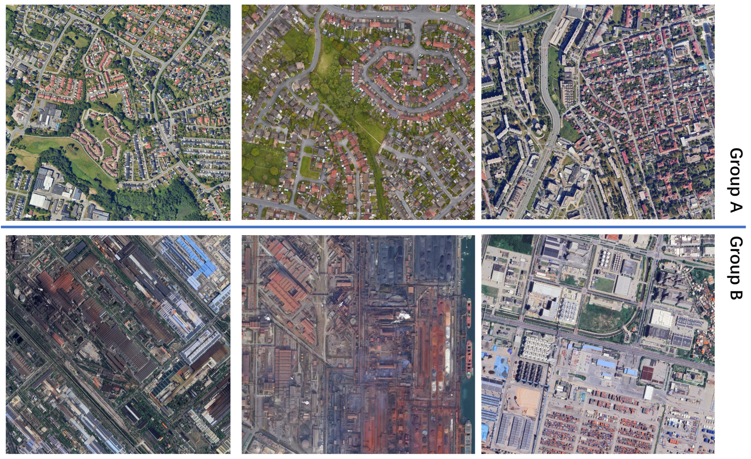
We use a concrete data example to illustrate the role of EMB. Figure 1 presents two groups of satellite images. Each group consists of three images from different geographic locations that exhibit similar EMB representations under the cosine distance metric. Group A shows comparable neighborhood appearances and building styles, indicating that these locations correspond to relatively affluent urban areas. Group B consists of images from port-adjacent heavy industrial zones. This example demonstrates that EMB encodings implicitly cluster regions with distinct economic characteristics even in the absence of labeled data.

Despite the above advantages, the EMB-based approach is subject to several limitations. First, EMB constitutes a high-dimensional, black-box representation, which limits the direct interpretability of the extracted features. Second, while EMB captures rich physical and structural characteristics of the Earth’s surface, it remains less sensitive to forms of economic activity that leave weak or delayed spatial footprints, such as services, finance, and digital production, particularly in high-income regions. Third, the open source GSED is updated at annual intervals, which leads to a temporal lag between real economic changes and their representation in the EMB space. This may reduce accuracy in contexts characterized by rapidly changing urban environments, infrastructure development, or short-term economic shocks. Fourth, the performance of EMB inherently depends on the training objectives, data coverage, and inductive biases of the underlying AEF model, which may introduce systematic dependencies on the composition and temporal scope of the satellite data used during pretraining. Since these limitations are partly structural, we recommend the joint use of EMB and more traditional NTL-based measures to capture long-term economic structure and short-term dynamics, respectively. As satellite embedding technologies continue to advance and more embedding generation models and datasets become openly available, some of these limitations may be mitigated in future applications.

2.2. Transfer Learning from NTL

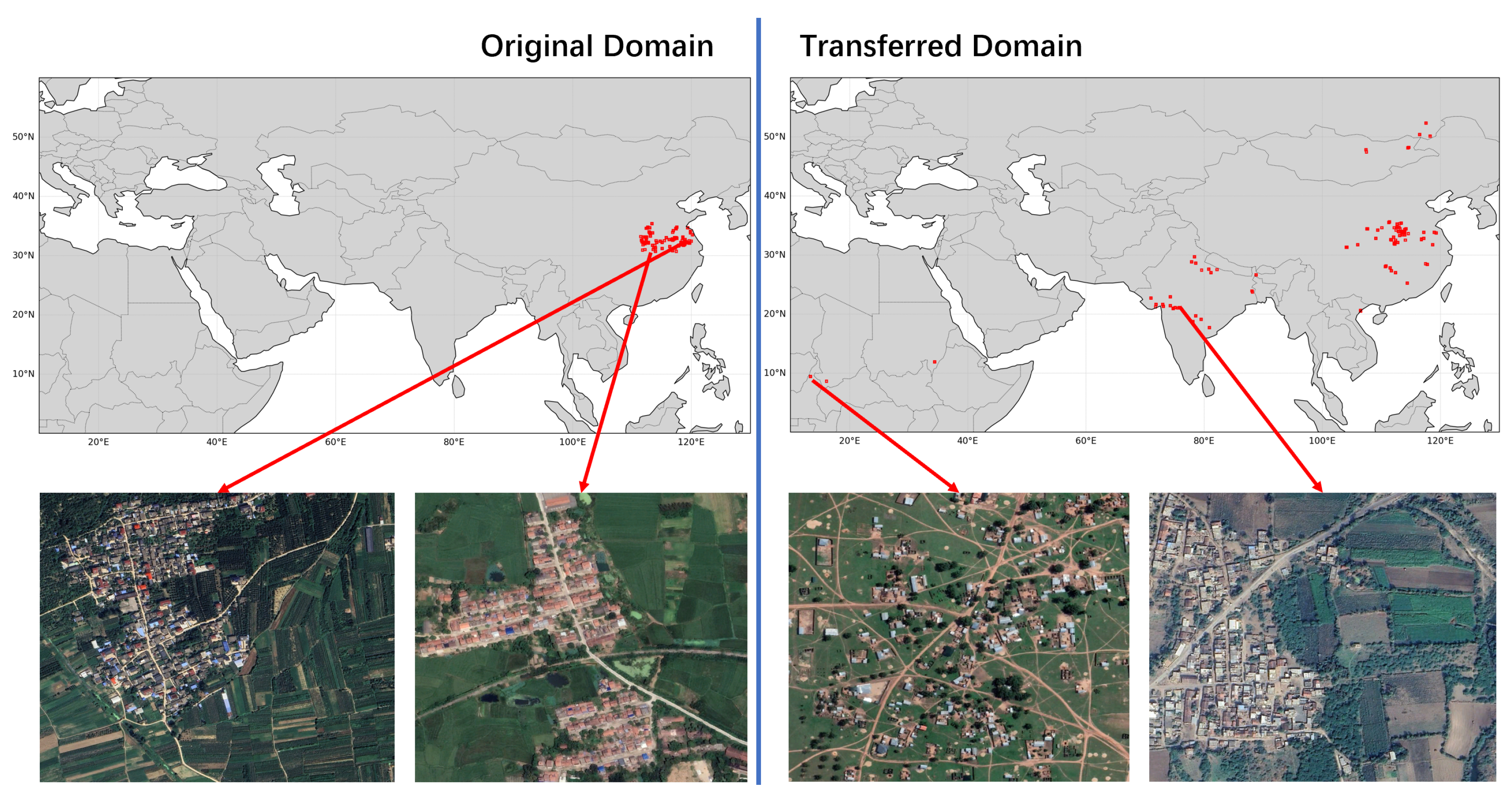
We focus on the economic information encoded in EMB representations. This assumption faces challenges when economically related features are intertwined with natural geographic characteristics. As illustrated in Figure 2, when we search for locations with similar EMB encodings to a rural area in the central plains of China within the original EMB domain, the top 100 candidate regions are all geographically proximate and share similar climatic patterns. In such cases, similarity in the embedding space is largely driven by natural environmental factors rather than economic structure. An effective feature representation for economic analysis should identify regions with similar economic characteristics across distant geographic locations. Since NTL data have been widely used as proxies for economic income, we employ transfer learning from EMB to NTL to separate economically relevant features from those that primarily reflect natural geography.

Let ${\mathbf{x}}_i\in {\mathbb{R}}^{64}$ denote the EMB vector for spatial unit i, derived from AEF model of daytime satellite observations that combine optical and radar imagery [35]. Each spatial unit also has an observed NTL intensity $y_i^{\left(NL\right)}$, taken from the Visible Infrared Imaging Radiometer Suite (VIIRS) onboard the Suomi National Polar-Orbiting Partnership (Suomi–NPP) satellite, preprocessed to annual means and aligned to administrative boundaries following [6,17].

We define a neural network $f_{\theta }:{\mathbb{R}}^{64}\to \mathbb{R}$ parameterized by $\theta$, trained to approximate the mapping

$${\widehat{y}}_i^{\left(NTL\right)}=f_{\theta }\left({\mathbf{x}}_i\right),$$

(1)

where ${\widehat{y}}_i^{\left(NTL\right)}$ denotes the predicted NTL. The parameters $\theta$ are estimated by minimizing the mean squared error (MSE) loss:

$${\mathcal{L}}_{NTL}\left(\theta \right)={\displaystyle \frac{1}{N}}\sum _{i=1}^N{\left(f_{\theta }\left({\mathbf{x}}_i\right)-y_i^{\left(NTL\right)}\right)}^2,$$

(2)

where $y_i^{\left(NTL\right)}$ represents the observed NTLs.

This step allows the model to align the spectral and structural information encoded in EMB with observable NTL intensity, effectively transferring the economic signal from nighttime to daytime satellite representations.

Once $f_{\theta }$ is trained, we truncate the network at an intermediate hidden layer to obtain a lower-dimensional representation. Let

$${\mathbf{z}}_i=g_{\theta }\left({\mathbf{x}}_i\right)\in {\mathbb{R}}^{32}$$

(3)

denote the output of the selected intermediate layer, where $g_{\theta }$ maps the 64-dimensional input to a 32-dimensional latent vector.

This economically aligned representation ${\mathbf{z}}_i$ retains features that are predictive of economic activity while filtering out redundant spectral details unrelated to the economy, e.g., spectral differences induced by vegetation. Figure 2 illustrates this effect. Compared with the original EMB representation, the reprojected embedding ${\mathbf{z}}_i$ captures regions with similar economic structures at a cross-continental scale. All highlighted regions are characterized by the coexistence of agricultural land and clustered rural settlements. The result indicates that the transfer learning process attenuates similarities driven by natural geography and emphasizes economically relevant spatial patterns.

2.3. GDP Prediction from Economic Embeddings

Based on the economically aligned representation ${\mathbf{z}}_i$s as input, we construct a country-level predictor of GDP by aggregating the economically enriched features obtained in the transfer learning stage. The GDP mapping network comprises two stages, as discussed below.

Let each spatial unit i within the country c be represented by its 32-dimensional economic embedding ${\mathbf{z}}_i\in {\mathbb{R}}^{32}$, produced by the truncated network $g_{\theta }(·)$ described above.

We first transform these features through a mapping network

$${\mathbf{v}}_i=p_{\psi }\left({\mathbf{z}}_i\right)\in {\mathbb{R}}^{16},$$

(4)

where $p_{\psi }$ is a feed-forward neural network parameterized by $\psi$. This step compresses and refines the spatial representation, encouraging the model to extract the most salient components for national-level income prediction.

Next, we aggregate these transformed vectors across all spatial units belonging to country c:

$${\mathbf{s}}_c=\sum _{i\in c}{\mathbf{v}}_i,$$

(5)

where ${\mathbf{s}}_c\in {\mathbb{R}}^{16}$ represents the summed national embedding vector that captures the cumulative economic structure observed in daytime imagery.

Finally, a country-level prediction network

$${\widehat{y}}_c^{\left(EMB\right)}=h_{\varphi }\left({\mathbf{s}}_c\right),$$

(6)

maps the aggregated representation to a scalar estimate of GDP. The parameters $\{\psi ,\varphi \}$ are jointly trained to minimize the mean squared error between predicted and official GDP:

$${\mathcal{L}}_{GDP}(\psi ,\varphi )={\displaystyle \frac{1}{C}}\sum _{c=1}^C{\left(h_{\varphi }\left(\sum _{i\in c}{p}_{\psi }\left({\mathbf{z}}_i\right)\right)-y_c^{\left(GDP\right)}\right)}^2,$$

(7)

where C is the number of countries, $y_c^{\left(EMB\right)}$ denotes the estimated (log-)GDP of country c by EMB, and $y_c^{\left(GDP\right)}$ denotes the official (log-)GDP of country c.

This hierarchical design ensures that the model first captures localized economic patterns at the spatial-unit level, then aggregates them into a coherent national representation, and finally learns a nonlinear mapping to aggregate income. By summing features before the final prediction stage, the framework respects additivity across spatial units and reduces overfitting to fine-scale noise.

2.4. Hybrid GDP Estimation

We construct a hybrid predictor of GDP as a convex combination of the two estimates to exploit the complementary strengths of EMB and NTL data:

$${\widehat{y}}_c^{\left(Hybrid\right)}=\lambda {\widehat{y}}_c^{\left(EMB\right)}+(1-\lambda ){\widehat{y}}_c^{\left(NTL\right)},$$

(8)

where ${\widehat{y}}_c^{\left(NTL\right)}$ denotes GDP predicted from a benchmark NTL-only model (as in [17] Hu et al. found that defining each country’s per capita NTL as total NTL divided by total population, per capita GDP and per capita NTL exhibit a quadratic relationship. This holds both when individual fixed effects are excluded and when they are included. The former corresponds to the estimation of GDP levels, and the latter to the estimation of GDP growth. The present study adopts this estimation framework), and $\lambda \in [0,1]$ can be optimized by evaluating validation performance over a discrete grid with a fixed step size. In this paper, we consider $\lambda$ values in increments of 0.25 to identify an approximate optimum. Since NTL and EMB estimate GDP from distinct data sources, they can be regarded as providing relatively independent information. Consequently, a linear combination of the two estimators may achieve better performance than either source alone.

2.5. Implementation Details

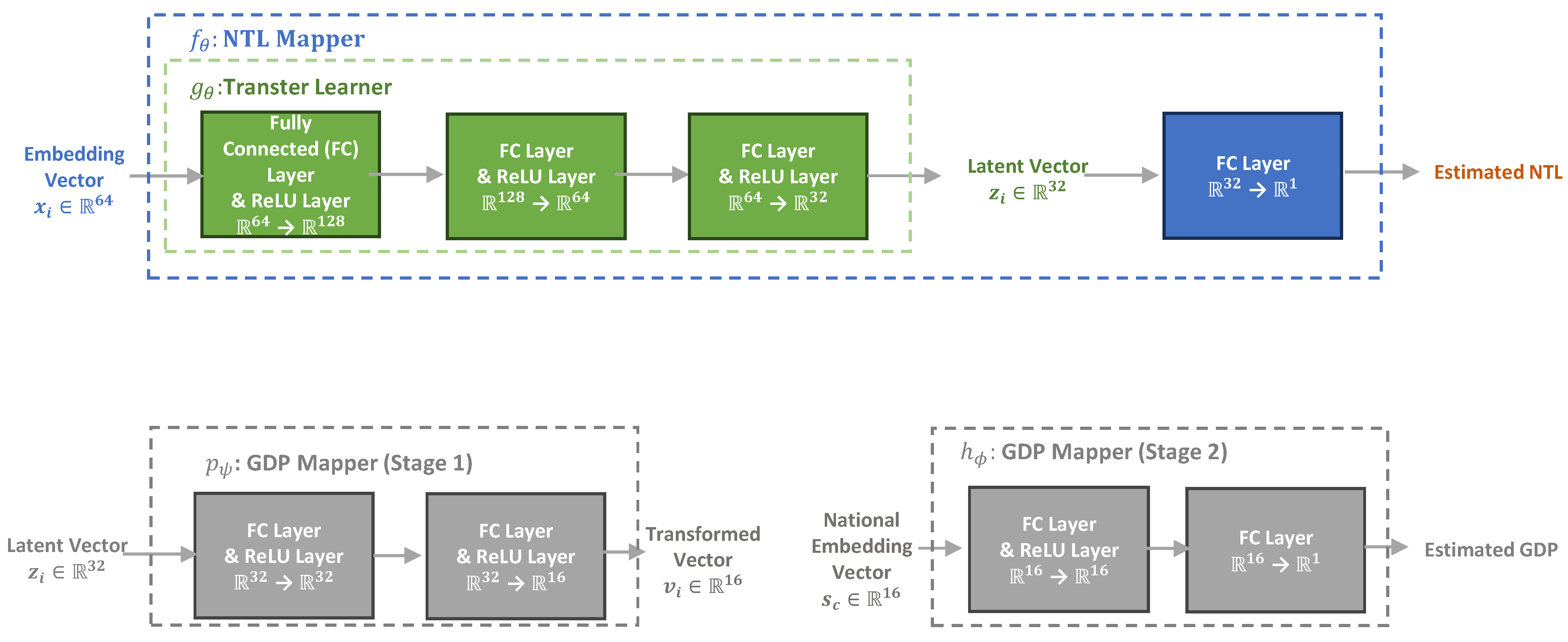
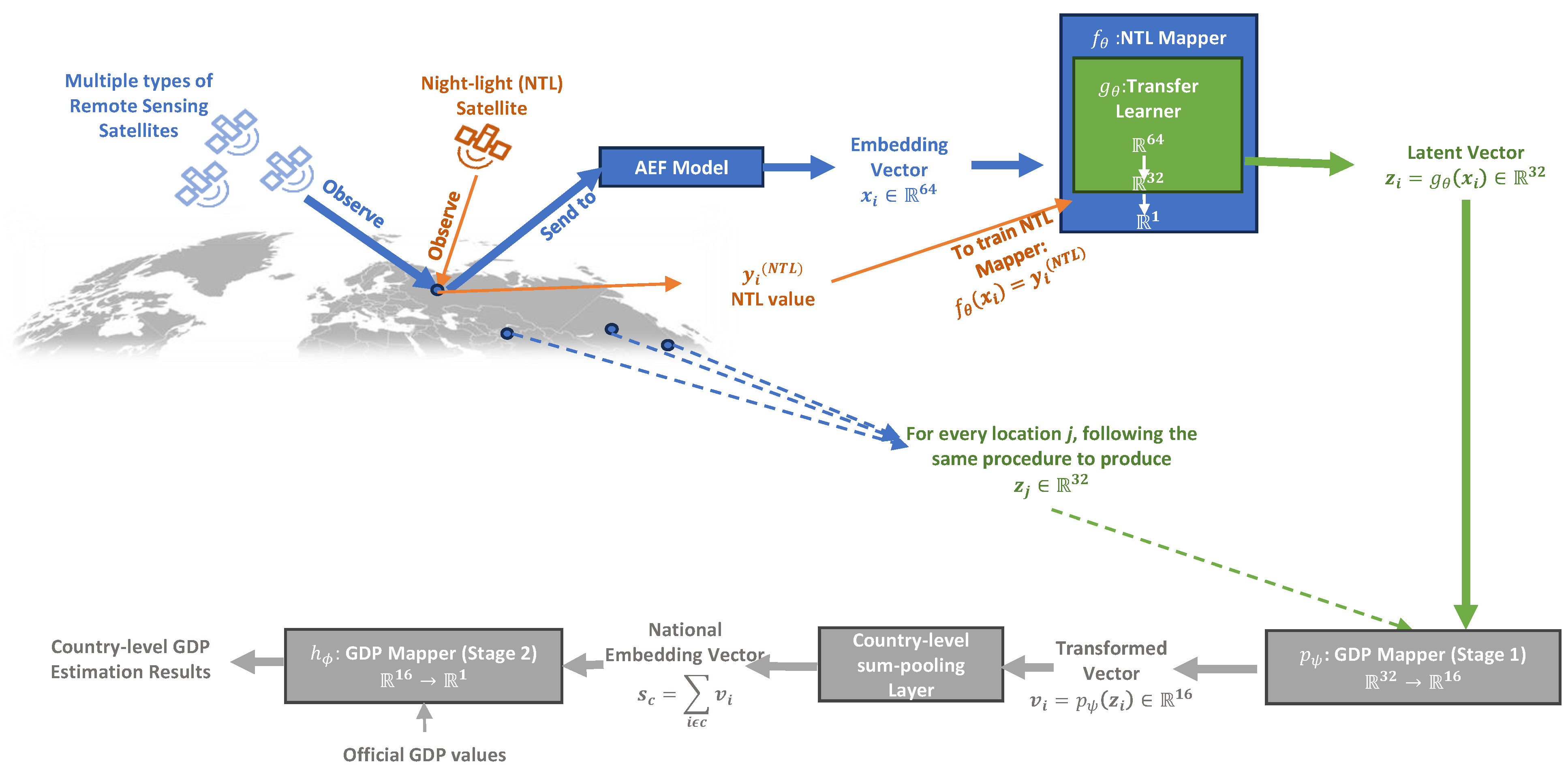
The overall neural network architecture is illustrated in Figure 3 and Figure 4. The training process is implemented following two sequential steps. In the first step, the NTL Mapper is trained according to the objective function defined in (2), learning the mapping from EMB to NTL intensity. In the second step, the two-stage GDP Mappers are jointly trained according to the objective function (7). This two-step design ensures that the model first captures economically relevant spatial signals in the embedding space and then efficiently transfers them to GDP representation learning.

All neural networks are implemented in PyTorch 2.5.1. For the first stage NTL mapper, the training uses the Adam optimizer with a fixed learning rate of 0.001 and stops after 10 epochs. The batch size is set to 32. For the GDP mapper, training is performed using the Adam optimizer with an initial learning rate of 0.001. The learning rate decreased to 0.0001 after 1100 epochs. The batch size is set to 32. An early stopping strategy is applied based on validation loss. Specifically, after a minimum of 1100 training epochs, the training process is terminated if the average validation loss over a rolling window of 100 epochs does not exhibit further improvement. The dataset is partitioned by country into training, validation, and testing subsets to ensure that no spatial unit appears in multiple partitions. Specifically, the full sample is divided into five mutually exclusive groups. In each rotation, one group is used for validation, one group is used for testing, and the remaining three groups are used for training. This procedure is repeated five times, rotating the roles of the groups, so that testing outputs are obtained for all samples and aggregated to produce comprehensive evaluation results.

2.6. Econometric Explanation

This subsection formalizes the econometric logic underlying the observed prediction errors within a conditional independence framework.

Let $y_{it}^{\left(true\right)}$ denote the latent true log GDP per capita of country i in year t, which is unobservable. The empirical analysis relies on officially reported GDP,

$$y_{it}^{\left(official\right)}=y_{it}^{\left(true\right)}+{\epsilon }_{it}^{\left(stat\right)},$$

(9)

where ${\epsilon }_{it}^{\left(stat\right)}$ denotes statistical measurement error generated by national accounting systems.

Satellite-based models aim to recover information about $y_{it}^{\left(true\right)}$ using observable remote sensing inputs. Let $y_{it}^{\left(sat\right)}$ denote satellite-derived information, such as NTL intensity or EMB-based representations. The relationship between satellite signals and true GDP can be expressed as

$$y_{it}^{\left(true\right)}=\mathrm{m}\left(y_{it}^{\left(sat\right)}\right)+{\epsilon }_{it}^{\left(sat\right)},$$

(10)

where $\mathrm{m}(·)$ is the true mapping from satellite information to economic output, and ${\epsilon }_{it}^{\left(sat\right)}$ captures the intrinsic limitation of satellite-based proxies. In this study, $sat$ takes values from $\{EMB,NTL\}$.

Combining the two equations yields the data-generating process for the observable outcome:

$$y_{it}^{\left(official\right)}=m\left(x_{it}\right)+{\epsilon }_{it}^{\left(sat\right)}+{\epsilon }_{it}^{\left(stat\right)}.$$

(11)

In practice, $\mathrm{m}(·)$ is approximated by an estimated model $\widehat{\mathrm{m}}(·)$ using either NTL- or EMB-based inputs. The empirical residual used to evaluate prediction performance is therefore

$${\epsilon }_{it}=y_{it}^{\left(official\right)}-\widehat{m}\left(x_{it}\right).$$

(12)

Assuming that $\widehat{\mathrm{m}}(·)$ consistently estimates $\mathrm{m}(·)$, the approximation error $\mathrm{m}\left(x_{it}\right)-\widehat{\mathrm{m}}\left(x_{it}\right)$ becomes asymptotically negligible, and the residual can be written as follows:

$${\epsilon }_{it}\approx {\epsilon }_{it}^{\left(sat\right)}+{\epsilon }_{it}^{\left(stat\right)}.$$

(13)

The two components of the residual arise from distinct data-generating mechanisms. Statistical measurement error ${\epsilon }_{it}^{\left(stat\right)}$ is driven by the quality of national statistical systems. The variance of ${\epsilon }_{it}^{\left(stat\right)}$ is heterogeneous across countries and depends on national statistical capacity. Satellite-based error ${\epsilon }_{it}^{\left(sat\right)}$ reflects the extent to which economic activity is observable from space. The magnitude of ${\epsilon }_{it}^{\left(sat\right)}$ is systematically related to the level of economic development. As economies develop, a larger share of GDP comes from service and digital sectors that are less visible in remote-sensing imagery. These two components may be correlated across countries because statistical capacity and income levels are themselves correlated. Our identifying assumption is therefore one of conditional independence. Let $S_i$ denote national statistical capacity (proxied by SPI), and let the log-transformed official per capita GDP ${\tilde{y}}_{it}^{\left(official\right)}$ serve as a proxy for the level of economic development. We assume

$${\epsilon }_{it}^{\left(stat\right)}\perp \perp {\epsilon }_{it}^{\left(sat\right)}\mid (S_i,{\tilde{y}}_{it}^{\left(official\right)}),$$

(14)

that is, conditional on statistical capacity and income level, the remaining variation in statistical measurement error is independent of the remaining variation in satellite-based error.

Under this assumption, the conditional dispersion of the observed residual satisfies the following:

$$\mathrm{Var}({\epsilon }_{it}\mid S_i,{\tilde{y}}_{it}^{\left(official\right)})=\mathrm{Var}({\epsilon }_{it}^{\left(stat\right)}\mid S_i)+\mathrm{Var}({\epsilon }_{it}^{\left(sat\right)}\mid {\tilde{y}}_{it}^{\left(official\right)}).$$

(15)

Finally, this study does not attempt to separately identify ${\epsilon }_{it}^{\left(stat\right)}$ and ${\epsilon }_{it}^{\left(sat\right)}$ or to recover the latent true GDP, although errors-in-variables approaches such as SIMEX could be employed for this purpose. We focus on taking EMB as a new data source for GDP estimation and assessing how its relative performance varies across countries with different statistical capacity and income levels. This conditional independence framework provides the theoretical foundation for the empirical results reported in Section 3, especially in Section 3.4.

3. Results

3.1. Dataset Preparation

The period of the EMB dataset spans 2017 to 2024, matching the temporal coverage of the released GSED. For NTL data, we employ the stable VIIRS–DNB composite series [42], available from 2014 to the present. We restrict our analysis to the intersection of the two time ranges (2017–2024) to ensure temporal consistency across both data sources.

As summarized in

Table 1. Data sources and pre-processing details.

Dataset	Pre-Processing Details
EMB data	Downloaded from the Google Earth Engine (GEE) platform, dataset ID: GOOGLE/SATELLITE_EMBEDDING/V1_ANNUAL;
	Years: 2017–2024; aggregated to a 10 km grid.
NTL data	VIIRS Nighttime Day/Night Annual Band Composites V2.2 from GEE;
	Years: 2017–2024; aggregated to the same 10 km grid as the satellite embedding dataset.
Official GDP per Capita	World Bank indicator “NY.GDP.PCAP.CD” (current USD, annual).
Official GDP Growth	World Bank indicator “NY.GDP.MKTP.KD.ZG” (annual growth rate, %).
Auxiliary layers	Administrative boundaries (GADM v4.0);
	Population (World Bank “SP.POP.TOTL”);
	Land-cover data (MODIS Land Cover Type Yearly Global 500 m, GEE platform).

, all satellite-derived datasets are spatially aggregated to a uniform 10 km grid. The EMB and NTL data are first resampled to this common resolution to ensure comparability. We then apply a land-cover mask derived from MODIS Land Cover Type data to exclude grid cells that are clearly unrelated to economic activity, such as water bodies, forested regions, glaciers, and deserts. Administrative boundary data from GADM 4.0 are used to assign each grid cell to its corresponding country.

This preprocessing step ensures that each grid cell can be linked to country-level economic statistics from the World Bank. Population data are used to convert predicted national aggregates into per capita terms, enabling direct comparison with official per capita GDP series.

3.2. Econometric Evaluation Strategy

We conduct two sets of evaluations: The estimation of GDP levels and the estimation of GDP growth. The evaluation strategy is designed to ensure consistency with the econometric framework described in the Section 2.

3.2.1. Estimation of GDP Levels

For the estimation of GDP levels, we compare the predictive performance of three approaches: the EMB-based estimator, the NTL-based estimator, and a mixed estimator that combines the two.

For the EMB approach, we first compute per capita values and directly assess the absolute levels of per capita GDP using the following validation regression:

$${\tilde{y}}_{it}^{\left(official\right)}=\alpha +\beta {\tilde{y}}_{it}^{\left(EMB\right)}+{\epsilon }_{it}^{\left(EMB\right)},$$

(16)

where ${\tilde{y}}_{it}^{\left(official\right)}$ denotes the log-transformed official per capita GDP for country i in year t, and ${\tilde{y}}_{it}^{\left(EMB\right)}$ refers to the log-transformed per capita GDP estimated from the EMB-based model. The error term ${\epsilon }_{it}^{\left(EMB\right)}$ captures the discrepancy between the EMB-derived estimates and official GDP statistics.

This regression is not intended to construct a new predictive model, but rather to serve as a validation exercise for the EMB-based estimates. Accordingly, ${\tilde{y}}_{it}^{\left(EMB\right)}$ is treated as a pre-computed model output, and the regression is used to assess its statistical alignment with official GDP data. The coefficient $\beta$ measures the proportional consistency between the EMB-based estimates and official GDP levels. $\beta$ is expected to be statistically indistinguishable from unity, while the intercept $\alpha$ is expected to be statistically indistinguishable from zero. Deviations from these values would indicate systematic level or scaling differences between the EMB-based estimates and official statistics. Model performance is evaluated by the mean squared error (MSE) of ${\epsilon }_{it}^{\left(EMB\right)}$ across all country–year observations.

For the NTL-based approach, we estimate a linear or quadratic predictive relationship between night light intensity and official per capita GDP:

$${\tilde{y}}_{it}^{\left(official\right)}=\alpha +{\beta }_1{\tilde{y}}_{it}^{\left(NTL\right)}+{\beta }_2{\left({\tilde{y}}_{it}^{\left(NTL\right)}\right)}^2+{\epsilon }_{it}^{\left(NTL\right)},$$

(17)

where ${\tilde{y}}_{it}^{\left(official\right)}$ denotes the log-transformed official per capita GDP for country i in year t, and ${\tilde{y}}_{it}^{\left(NTL\right)}$ represents the log-transformed per capita night light intensity for country i in year t. The error term ${\epsilon }_{it}^{\left(NTL\right)}$ captures the deviation of the NTL-based prediction from official GDP values. The inclusion of the quadratic term is optional to capture potential nonlinearities in the relationship between night lights and economic activity. When ${\beta }_2$ is set to zero, the specification reduces to a linear predictive model.

This regression is used as a predictive model rather than a causal model. ${\beta }_1$ reflects the average linear sensitivity of predicted GDP to changes in NTL intensity, while ${\beta }_2$ captures deviations from linearity, such as saturation effects at high or low light levels. Model performance is evaluated primarily by the MSE of ${\epsilon }_{it}^{\left(NTL\right)}$ across all country–year observations.

For the mixed estimator, we construct a convex combination of the EMB and NTL predictions, parameterized by $\lambda \in \{0.25,0.5,0.75\}$, and assess the MSE to identify potential efficiency gains from combining the two data sources.

3.2.2. Estimation of GDP Growth

To evaluate the models’ ability to capture within-country economic dynamics, we extend the analysis to GDP growth estimation. Specifically, we compare the performance of EMB-based, NTL-based, and mixed estimators within a fixed-effects (FEs) panel framework.

We estimate the following fixed-effects specification to assess the ability of satellite-based estimates to capture within-country variations in economic activity:

$${\tilde{y}}_{it}^{\left(official\right)}=\alpha +{\beta }_1{\tilde{y}}_{it}^{\left(sat\right)}+{\beta }_2{\left({\tilde{y}}_{it}^{\left(sat\right)}\right)}^2+{\gamma }_i+{\epsilon }_{it}^{(sat,FE)},$$

(18)

where ${\tilde{y}}_{it}^{\left(official\right)}$ denotes the log-transformed official per capita GDP for country i in year t, and ${\tilde{y}}_{it}^{\left(sat\right)}$ represents the log-transformed per capita GDP proxy derived from satellite data, including either EMB-based or NTL-based estimates. $sat\in \{\mathrm{NTL},\mathrm{EMB}\}$ corresponds to NTL-based and EMB-based estimates, respectively. The country fixed effects ${\gamma }_i$ absorb all time-invariant cross-country differences, such as persistent institutional characteristics or long-run income levels, while the constant term $\alpha$ captures the average level effect common across countries.

The inclusion of the quadratic term is optional and allows for potential nonlinearities in the relationship between satellite-based proxies and economic activity. When ${\beta }_2$ is set to zero, the specification reduces to a linear fixed-effects model. This specification is intended as a predictive framework rather than a causal model. After removing time-invariant country-specific components, the coefficient(s) ${\beta }_1$ (and ${\beta }_2$, when included) capture the extent to which within-country temporal variations in satellite-based measures are aligned with corresponding variations in official GDP. The residual term ${\epsilon }_{it}^{(sat,FE)}$ reflects remaining within-country discrepancies between satellite-based proxies and official statistics. Model performance is evaluated by the MSE of ${\epsilon }_{it}^{(sat,FE)}$ across all country–year observations.

Finally, for the mixed estimator, we construct linear combinations of EMB- and NTL-based predictions using weighting parameters $\lambda \in \{0.25,0.5,0.75\}$, and evaluate performance by the mean squared error (MSE) of residuals.

Including country and year fixed effects effectively removes persistent cross-sectional heterogeneity and common temporal shocks and isolates the within-country temporal variation in GDP. As a result, this FE specification makes the regression models in formula (18) to be interpreted as estimators of GDP growth rather than GDP levels.

3.3. Evaluation Results

Table 2. Validation regressions for satellite-based GDP proxies.

	GDP Level			GDP Growth (FE)
	NTL (Lin.)	NTL (Quad.)	EMB (Lin.)	NTL (Lin.)	NTL (Quad.)	EMB (Lin.)
Satellite proxy (${\tilde{y}}_{it}^{\left(sat\right)}$)	0.698 ***	1.032 ***	0.986 ***	0.228 ***	0.779 ***	0.028 **
	(0.013)	(0.182)	(0.014)	(0.022)	(0.138)	(0.011)
Satellite proxy2	–	0.014 *	–	–	0.023 ***	–
		(0.008)			(0.006)
Constant	16.520 ***	18.429 ***	0.020	−12.293 ***	−9.745 ***	−21.576 ***
	(0.146)	(1.047)	(0.123)	(2.536)	(2.597)	(2.484)
Observations	1225	1225	1225	1225	1225	1225
$R^2$	0.707	0.708	0.756	0.996	0.996	0.996
Fixed effects	No	No	No	Country	Country	Country

Notes: Each column reports a separate validation regression. Standard errors are reported in parentheses. ***, **, and * denote significance at the 1%, 5%, and 10% levels, respectively.

reports results of regressions (16)–(18) that assess the statistical alignment between satellite-based proxies and official GDP outcomes at both the level and growth dimensions.

The first column of Table 2 reports the linear NTL-based level regression. The estimated coefficient on the NTL proxy is positive and highly significant, indicating a strong monotonic association between NTL and official GDP levels. The second column extends the NTL-based level regression by allowing for a quadratic term. The linear coefficient remains highly significant, while the quadratic term is weakly significant, indicating mild nonlinearities in the mapping from NTL to income.

The third column reports the EMB-based level regression. In this specification, the linear coefficient is highly significant and statistically indistinguishable from unity. This pattern indicates that the EMB-based estimator is approximately unbiased with respect to official GDP levels.

Columns four and five report the NTL-based growth regressions with country fixed effects. In the linear specification (column four), the NTL proxy remains highly significant, indicating that within-country variation in NTL intensity is closely aligned with GDP growth. Column five allows for a quadratic term and shows that the quadratic coefficient is strongly significant.

The final column reports the EMB-based growth regression with country fixed effects. The estimated coefficient is positive and statistically significant but smaller in magnitude than in the corresponding level regression specifications. This result indicates that embedding-based measures are more suitable for capturing longer-term structural changes in economic activity than short-run fluctuations.

Finally, the high $R^2$ values in the fixed-effects regressions primarily reflect the explanatory power of country fixed effects in absorbing persistent cross-country income differences and should not be interpreted as evidence of superior predictive performance. Model comparison in the subsequent analysis relies on MSE rather than on $R^2$.

Additional robustness checks for these results are presented in Appendix A.

Table 3. Estimation results for GDP levels (MSE).

Estimator	Specification	$\mathit{\lambda }$	MSE
EMB	Direct level estimation	—	0.5037
NTL	Quadratic regression	—	0.6017
Mixed (EMB+NTL)	Linear combination	0.25	0.5101
		0.50	0.4620
		0.75	0.4594

shows the MSEs for the estimation of GDP levels. Based on the validation regressions reported in Table 2, we select the MSE reported in the linear form of the NTL-based models. The comparison of MSE values shows that EMB consistently achieves lower estimation error than NTL when predicting the absolute level of per capita GDP. The mixed estimator yields further improvements, with the smallest MSE observed at $\lambda =0.75$. This result indicates that combining EMB and NTL information leads to more accurate aggregate income estimation.

The estimation results of GDP growth are summarized in

Table 4. Estimation results for GDP growth (MSE).

Estimator	Specification	$\mathit{\lambda }$	MSE
EMB	FE regression	—	0.00836
NTL	Quadratic FE regression	—	0.00752
Mixed (EMB+NTL)	Linear combination	0.25	0.00757
		0.50	0.00780
		0.75	0.00797

. Based on the validation regressions reported in Table 2, we select the MSE reported in the quadratic form of the NTL-based models. The EMB-based fixed effects regression attains a slightly higher MSE than the NTL-based quadratic FE specification, implying that NTL captures short-run variations more effectively. The mixed estimator produces MSEs lying between those of the two individual models.

Overall, these results confirm the following two facts. Firstly, the EMB-based model yields more accurate estimates for GDP levels while the NTL-based model remains competitive for growth estimation due to its temporal sensitivity. Secondly, the mixed estimators achieve the lowest MSE in level estimation, especially when EMB receives a larger weight ($\lambda =0.75$).

Although prediction errors are heteroskedastic across countries, overall MSE remains a meaningful performance metric because all estimators are evaluated on the same sample with identical distributions of statistical capacity and income levels.

3.4. The Determinants of the Estimation Performance

This section discusses the determinants of the estimation performance. We analyze how the prediction errors of the four models (EMB-level, NTL-level, EMB-growth, and NTL-growth) vary with country characteristics. Specifically, we focus on two potential explanatory factors: (i) national statistical capacity and (ii) per capita income.

We begin with two hypotheses derived from the discussion in Section 2.6 and Equation (15):

H1. 

Prediction errors decrease with higher statistical capacity. The official GDP itself contains measurement errors, especially in low statistical capacity countries. The observed discrepancy between estimated and official GDP thus reflects both model error and statistical error, as demonstrated in Equation (15). In countries with stronger statistical systems, $\mathrm{Var}({\epsilon }_{it}^{\left(stat\right)}\mid S_i)$ is expected to be smaller, reducing the observed error.

H2. 

Prediction errors increase with income level. As economies develop, a larger share of GDP comes from service and digital sectors that are less visible in remote-sensing imagery. Thus, both NTL and EMB may exhibit larger residuals $\mathrm{Var}({\epsilon }_{it}^{\left(sat\right)}\mid {\tilde{y}}_{it}^{\left(official\right)})$ for high-income countries. EMB encoded rich daytime information, such as building quality and land use. Therefore, EMB-based models may mitigate this limitation relative to NTL.

To test these hypotheses, we regress the absolute residuals of each estimator on two explanatory variables: (i) the World Bank’s Statistical Performance Indicators (SPI) index [43], which is the proxy of national statistical capacity and (ii) the log of official GDP per capita. The empirical regression used to assess the determinants of residual dispersion is specified as follows:

$$\left|{\epsilon }_{it}\right|=\alpha +{\beta }_1{S}_i+{\beta }_2{\tilde{y}}_{it}^{\left(official\right)}+u_{it},$$

(19)

where $S_i$ denotes national statistical capacity, proxied by the Statistical Performance Indicators (SPI), and ${\tilde{y}}_{it}^{\left(official\right)}$ denotes the log-transformed official per capita GDP for country i in year t, serving as a proxy for the level of economic development. The dependent variable $\left|{\epsilon }_{it}\right|$ represents the absolute residual from the satellite-based GDP estimation, which aggregates both statistical measurement error and satellite-based observability error. We estimate this model separately for each of the four experimental settings: EMB-level (${\epsilon }_{it}={\epsilon }_{it}^{\left(EMB\right)}$), NTL-level (${\epsilon }_{it}={\epsilon }_{it}^{\left(NTL\right)}$), EMB-growth (${\epsilon }_{it}={\epsilon }_{it}^{(EMB,FE)}$), and NTL-growth (${\epsilon }_{it}={\epsilon }_{it}^{(NTL,FE)}$). The regression is not intended to identify a causal relationship. Instead, log GDP per capita is used as a state variable to index heterogeneity in the conditional dispersion of prediction errors.

Table 5. Regression of absolute residuals on SPI and income level.

	Level Estimation		Growth Estimation
	EMB	NTL	EMB	NTL
SPI index	−0.0027 **	−0.0005	−0.0017 ***	−0.0017 ***
Log(GDP per capita)	+0.0398 ***	+0.1048 ***	+0.0084 ***	+0.0090 ***
Constant	0.4063 ***	−0.2702 ***	0.1032 ***	0.0949 ***
Observations	1225	1225	1225	1225
F-statistic	6.485	59.23	46.09	50.42
Prob(F)	0.001	2.8 × ${10}^{-25}$	5.1 × ${10}^{-20}$	9.1 × ${10}^{-22}$

Notes: The dependent variable is the absolute residual $|{\epsilon }_{it}|$. Coefficients marked *** $p<0.01$, ** $p<0.05$, * $p<0.1$.

reports the estimated coefficients and significance levels.

The results indicate that the SPI index exerts a consistently negative influence on prediction errors, confirming hypothesis H1. The negative effect is statistically significant in all cases except when per capita NTL is used to estimate absolute GDP levels, where the coefficient becomes insignificant. The reason for the insignificance may be the greater idiosyncratic noise inherent in NTL measurements.

For hypothesis H2, our results support that the log of per capita income is positively correlated with estimation errors in all cases, and the effect is notably stronger for NTL-based estimates. Compared with NTL-based models, EMB-based models are less sensitive to income differences.

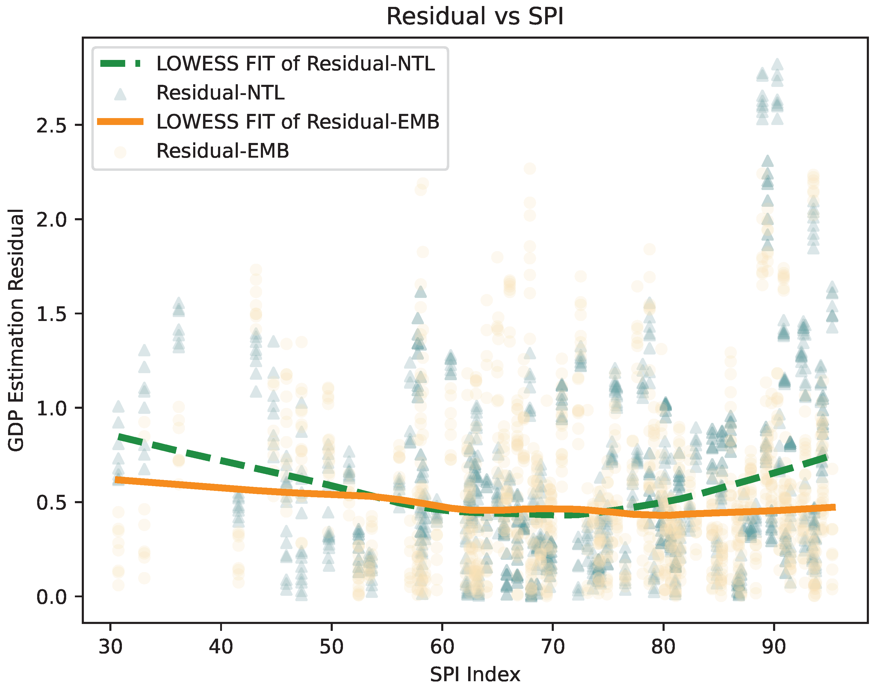
We further plot the expected prediction error as a function of the SPI index, as shown in Figure 5. The curve shows that, across both low- and high-statistical-capacity countries, EMB consistently achieves lower estimation errors than NTL for GDP levels. This result suggests that the EMB-based approach provides a more robust representation of economic structure across diverse institutional contexts. Therefore, we recommend using EMB or a mixed EMB+NTL estimator when assessing true GDP levels in both low-income and high-income regions, where statistical quality and the structure of economic activity differ substantially.

Figure 5 illustrates how prediction errors vary with statistical capacity when averaging over countries at different income levels. Under our conditional independence framework, a well-behaved estimator should exhibit declining errors as statistical capacity improves, with residuals converging to the model’s intrinsic satellite-based error. The EMB-based estimator closely follows this pattern, while the NTL-based estimator deviates at high SPI levels due to its increasing sensitivity to income-related structural features.

These results collectively indicate that EMB outperforms NTL in estimating absolute economic levels, particularly at both ends of the spectrum—countries with low statistical capacity and high-income economies. For the former, prior research has recommended using NTL instead of official statistics to approximate true income levels. Our findings suggest that the proposed EMB-based models, or their combination with NTL, can yield more reliable estimates. For the latter countries with high per capita income but weak statistical capacity, EMB remains preferable, as it exhibits sufficiently lower statistical errors in high-income contexts compared with NTL. Moreover, when extending income estimation to smaller spatial units, the advantage of EMB becomes more pronounced due to its higher spatial resolution.

In contrast, NTL-based models are more suitable for measuring growth dynamics, as indicated by the test results discussed above.

3.5. Application on Estimating True GDP Levels Across Countries

We apply the trained models (EMB, NTL, and their combination) to estimate country-level GDP from 2017 to 2024. For each country i and year t, we compute the predicted GDP per capita ${\widehat{y}}_{it}^{\left(sat\right)}$ and compare it with the official World Bank statistics $y_{it}^{\left(\mathrm{official}\right)}$. The relative deviation is defined as follows:

$${\mathrm{Deviation}}_{it}={\widehat{y}}_{it}^{\left(sat\right)}-y_{it}^{\left(\mathrm{official}\right)}.$$

(20)

Countries with persistently positive deviations may have underreported GDP or unmeasured informal activity, whereas those with persistently negative deviations may have potentially overreported official GDP. To identify the latter cases, we focus on the subset of countries with the lowest 25% of the Statistical Performance Index (SPI), as these countries typically exhibit weaker national accounting systems and lower reliability of official economic statistics.

Table 6. Countries in the lowest 25% SPI group with potentially overestimated GDP levels (Top 10).

Country	Official $log\left({\mathit{GDP}}_{\mathit{pc}}\right)$	Predicted $log\left({\mathit{GDP}}_{\mathit{pc}}^{\mathit{EM}1}\right)$	Difference
Oman	9.8020	8.5077	−1.2943
Papua New Guinea	7.8260	6.8315	−0.9946
Angola	7.8334	7.0159	−0.8175
Guyana	9.3443	8.5372	−0.8071
Kuwait	10.1594	9.8151	−0.3443
Timor-Leste	7.3007	7.0395	−0.2613
Turkmenistan	8.8672	8.6321	−0.2352
Lebanon	8.8394	8.7122	−0.1272
Democratic Republic of the Congo	6.2062	6.1135	−0.0928
Cameroon	7.2845	7.1962	−0.0884

lists the top ten countries with the largest negative deviations between predicted and official GDP levels in 2024 in the lowest-SPI group. Oman, Papua New Guinea, and Angola show more than 0.8 in log points. The results suggest that their officially reported per capita GDP levels may exceed those implied by the EMB-based estimates. Similarly,

Table 7. Countries in the lowest 25% SPI group with potentially overestimated GDP growth (top 10, 2017–2024 cumulative % change).

Country	Official Growth (%)	Predicted Growth (NTL-FE, %)	Difference (pp)
Guyana	284.9	19.9	−265.0
Sudan	86.1	7.9	−78.2
Timor-Leste	62.1	10.0	−52.1
Afghanistan	48.9	7.0	−41.9
Libya	63.9	21.6	−42.3
Turkmenistan	26.6	4.1	−22.5
Bahamas	33.1	10.5	−22.6
Angola	24.7	5.0	−19.7
China	35.4	17.1	−18.3
Democratic Republic of the Congo	16.2	5.5	−10.7

presents the top ten countries with the largest negative deviations in cumulative GDP growth from 2017 to 2024 inferred from the NTL-FE approach. Countries such as Guyana, Sudan, and Timor-Leste exhibit official growth rates far higher than those estimated from satellite data. Although the magnitudes should not be interpreted literally as mismeasurement rates, these deviations may indicate cases where national statistics diverge from physical and activity-based proxies.

4. Discussion

The results of the experiments indicate that the EMB-based GDP estimates achieve substantially higher accuracy than the NTL-based estimates in predicting GDP levels. Figure 5 provides a detailed comparison of their respective performance. We offer the following additional interpretation of the patterns shown in the figure. A well-behaved GDP-level estimator should exhibit a monotonic decline in prediction error as SPI increases. Lower SPI values imply that official GDP statistics are less reliable, so prediction errors derived from satellite-based models will reflect both the noise embedded in official GDP figures and the intrinsic modeling error of the satellite-based estimator. Conversely, higher SPI values indicate that official statistics are closer to true GDP, in which case the observed prediction error should primarily reflect the model’s own estimation error. In our results, the EMB-based estimator conforms more closely to this ideal error pattern. By contrast, the NTL-based curve exhibits pronounced upward deviations at both low-SPI and high-SPI ranges, resulting in a U-shaped pattern. This suggests that the prediction error of the NTL-based model with respect to true GDP (not official GDP) is not stable across SPI levels. The possible explanation is that NTL data contain systematically larger prediction errors in both low-income and high-income economies, and income levels are positively correlated with SPI. Taken together, these findings further demonstrate that EMB-based GDP estimators display more desirable statistical properties, with estimation errors that do not require adjustment for cross-country differences in income levels.

It is important to clarify the scope and interpretation of the estimation results of true GDP levels across countries. The country lists above were obtained by ranking residuals only within the subset of nations whose SPI values fall in the bottom 25% globally. In low-SPI contexts, national accounts may be less reliable, and independent validation from remote-sensing proxies becomes more meaningful. By contrast, ranking residuals across all countries would be difficult to interpret, since deviations in high-income economies are more likely driven by limitations of the remote-sensing proxies themselves rather than by deficiencies in statistical capacity. Accordingly, these findings should be interpreted as identifying candidates in which official GDP levels or growth might be overestimated, not as definitive evidence of mismeasurement or as proof of the model’s superiority. The EMB and NTL-based estimators serve here as independent diagnostic tools that highlight where further scrutiny may be warranted. Large negative deviations (official > predicted) could arise from several mechanisms, such as infrequent base-year revisions, inflation misreporting, valuation differences in resource exports, or partial coverage of informal activity. Each of these explanations is context-specific and cannot be confirmed without supplementary data.

In summary, this exercise demonstrates how learned geospatial features can be used as a screening tool for statistical validation in countries with weak statistical systems. It does not aim to rank or assess model accuracy across all economies but rather to flag cases where physical and administrative indicators diverge substantially and may merit closer investigation by statistical agencies and researchers.

5. Conclusions

This study demonstrates the potential of EMB as an advanced alternative to traditional NTL data for measuring economic activity from space. By transferring learned representations from daytime optical and radar imagery to the NTL domain, an “income-aware” embedding is constructed to capture structural and spatial patterns relevant to GDP estimation. Empirical results show that the EMB-based model achieves higher accuracy in estimating GDP levels, particularly in low-statistical-capacity or high-income countries, whereas NTL remains more responsive to short-term growth fluctuations.

Unlike earlier studies such as Henderson et al. [6] and Hu et al. [17], this paper does not attempt to systematically integrate official and model-predicted GDP series, as the current understanding of EMB is still preliminary. Future research may extend this direction by combining official data with embedding-based estimates to construct improved hybrid indicators.

Furthermore, embedding frameworks such as AEF could be enhanced by incorporating additional geospatial and socioeconomic signals, such as carbon emissions, transportation networks, logistics activity, and mobile phone data, into their latent representations. Such multi-source embeddings would enable more powerful, interpretable, and real-time models for global economic monitoring and policy analysis.