Article

Intelligent Fleet Monitoring System for Productivity Management of Earthwork Equipment

Department of Civil and Environmental Engineering, Hanyang University, Seoul 04763, Republic of Korea
*
Authors to whom correspondence should be addressed.
These authors contributed equally to this work as first authors.
These authors also contributed equally to this work.
Appl. Sci. 2026, 16(2), 1115; https://doi.org/10.3390/app16021115
Submission received: 23 December 2025 / Revised: 9 January 2026 / Accepted: 18 January 2026 / Published: 21 January 2026
(This article belongs to the Special Issue Building Information Modelling: From Theories to Practices)

Abstract

Earthwork operations constitute a substantial share of infrastructure project costs and are critical to overall project efficiency. However, the construction industry still relies on conventional approaches and there is a lack of integrated fleet management systems for collaboratively working equipment. While telematics is widely used in other industries, its applications to monitor the complex interactions between excavators, dump trucks, and dozers in real time remain limited. This study proposes an intelligent fleet monitoring system that utilizes only satellite navigation data (GNSS) to analyze the real-time productivity of multiple earthwork machines without relying on additional sensors, such as IMU or accelerometers, thereby eliminating the need for separate measurement procedures. A lightweight site configuration step is required to define the work area/loading/dumping geofences on an existing site map. This research provides novel developed algorithms that facilitate a real-time productivity assessment for several earthwork equipment and provide planning-level recommendations for equipment deployment combinations. Dedicated motion classification algorithms were developed for excavators, dump trucks, and dozers to distinguish activity states, to compute working and idle times, and to quantify operational efficiency. The system integrates a web-based e-Fleet Management platform and a mobile e-Map application for visualization and equipment optimization. Field validation was conducted on two active earthwork projects to evaluate accuracy and feasibility. The results demonstrate that the developed algorithms achieved classification and productivity estimation errors within 2.5%, while enabling optimized equipment combinations and improved cycle time efficiency. The proposed system offers a practical, sensor-independent approach for enhancing productivity monitoring, real-time decision-making, and cost efficiency in large-scale earthwork operations.

1. Introduction

The global construction industry shows an upward trend with consistent annual growth, with an estimated total size of USD 15 trillion by 2025 and USD 17.5 trillion by 2030 [1]. Earthwork typically accounts for a significant portion of an infrastructure project’s cost, such as in road and railway projects, and it can represent up to 30–50% of the total costs [2]. Despite numerous efforts to enhance the productivity of construction and infrastructure projects in recent years, the industry continues to grapple with slow productivity growth [3,4]. Most construction projects possess uncertain, dynamic, and transient characteristics, making it challenging to pinpoint the factors affecting productivity.
Currently, earthwork operations still depend heavily on the experiential judgment of managers and operators rather than data-driven monitoring systems [5,6]. The lack of integrated and collaborative fleet management often leads to inefficient equipment utilization, idle time, and inconsistent productivity. One of the most prominent technologies in other industries is fleet telematics, which has been successfully adopted in logistics and transportation for real-time tracking, maintenance, and operational control [7]. However, its use in the construction industry remains limited, particularly for the integrated management of multiple earthwork equipment working simultaneously on site. The majority of earthwork operations heavily rely on construction machinery and equipment, such as excavators, dump trucks, dozers, and rollers [8]. They must be selected and optimized based on the construction method, efficiency, and working conditions required for the specific project [9,10]. Earthwork operations typically involve multiple sequential tasks, such as excavation, transportation, spreading, compaction, and ground improvement, which are often intermixed [11].
Recent trends in the logistics and transportation industry have shown a significant increase in adopting fleet telematics technology for the safe and efficient management of fleets [12]. This technology enables the real-time sharing of fleet information, including location, operational status, fuel management, vehicle maintenance, driver management, and dispatch planning control [13,14]. Fleet management using telematics has been successfully implemented in logistics and transportation companies, resulting in improved efficiency, productivity, cost-effectiveness, and safety [15,16]. Previous studies have primarily focused on the unit productivity analysis of individual machines, such as excavators or dump trucks, without considering the overall earthwork process that includes excavation, hauling, and grading. Furthermore, most research has relied on multiple sensors, such as IMUs, gyroscopes, and accelerometers, which increases the complexity, cost, and calibration requirements, limiting scalability and field applicability [17]. Despite these advancements, several research gaps remain that restrict the practical implementation of fleet telematics in construction. Existing telematics frameworks depend on multiple sensing modules, resulting in higher costs and reduced flexibility for deployment under varying field conditions. Moreover, real-time productivity monitoring and optimization across the entire earthwork process have yet to be explored and comprehensively validated through practical on-site testing.
To address these limitations, this research aims to develop an intelligent fleet monitoring system for the real-time productivity analysis and management of the entire earthwork process using only Global Navigation Satellite System (GNSS) data. The proposed system utilizes advanced motion classification algorithms to calculate productivity and to provide planning-level equipment deployment guidance using GNSS-derived cycle-time information. By eliminating the need for additional sensors or survey data, it simplifies implementation while maintaining high accuracy and consistency and requiring only a lightweight site configuration based on geofence definition on existing BIM/GIS maps. The developed system integrates a web-based “e-Fleet Management” platform and a mobile “e-Map” application to visualize the equipment status, work type, and productivity of individual machines in real time. The evaluation and feasibility of the system were verified through field validation on two active earthwork projects.
The key contributions of this study are summarized as follows:
  • Development of motion classification algorithms for excavators, dump trucks, and dozers based solely on the GNSS data combined with user-defined geofences, without auxiliary sensors.
  • Implementation of a unified web-mobile fleet management platform for real-time productivity visualization and optimization.
  • Validation of the developed system through two field case studies demonstrating accuracy within 2.5% for productivity estimation, confirming its reliability and practical applicability.
Overall, this study establishes a scalable and sensor-independent framework for intelligent fleet management, supporting data-driven productivity monitoring and decision-making in earthwork operations.

2. Literature Review

It is essential to examine the potential of fleet telematics in improving the productivity of earthwork operations in the construction industry. The goal of applying fleet telematics for earthwork operations is to optimize operational efficiency by introducing intelligent systems that streamline processes such as loading, hauling, dispatching, tracking, and planning in real time. A substantial body of literature has been published analyzing the unit productivity of construction equipment using various sensing technologies, including GPS, IMU, accelerometers, gyroscopes, and audio-based systems. To assess the current status of fleet telematics in earthwork applications, it is necessary to review the existing research and to identify the key challenges that hinder widespread implementation. Accordingly, this section provides background information and relevant strategies in fleet telematics and identifies critical research gaps that must be addressed to advance its practical use in construction.

Fleet Telematics Technology

Fleet telematics technology falls under the umbrella of the supply chain industry. It enables communication via satellite and terrestrial wireless networks across logistics, transportation, and distribution systems to improve operational productivity, service quality, and cost efficiency [18,19]. Telematics technology has been introduced in the construction industry and focuses on closely monitoring and optimizing the efficiency of excavators and dump trucks with a series of sophisticated sensing technologies, such as GPS, IMU, gyroscopes, and accelerometers. For the last two to two-and-a-half decades, the construction equipment industry has been working to adopt fleet telematics to improve productivity, operations, maintenance, and management for earthwork operations. Construction fleet telematics can be divided into four major components, each with its own principal functions: (i) Collection and Buffering, it collects and stores data from different sensors, including GPS information, for later transmission; (ii) Transmission and Receipt, it sends the data to a centralized location based on the most cost-effective technology available; (iii) Processing and Archiving, it processes the received data to generate reports and to manage data flow; (iv) Dissemination and Use, it disseminates the reports and charts to the construction manager for an effective understanding of fleet requirements and decision making [20]. It is worth noting that the capabilities of fleet telematics extend beyond simple equipment location tracking [21]. The Association of Equipment Management Professionals (AEMP) has established a standard for telematics data that allows the monitoring of equipment without the requirement of specialized sensors [20]. However, to apply this to construction equipment, it is necessary to establish connections between the relevant modules, such as the engine, transmission, and brakes, and the response device via the CAN bus protocol. Notably, not all manufacturers support this standard protocol [22]. Additionally, even though the CAN bus protocol can be connected, the data are often encrypted for security reasons, which poses a significant challenge to scalability during on-site deployment and integration across different equipment brands. Recent studies have also emphasized that standardization and interoperability remain major bottlenecks for industry-wide implementation [23,24].
Fleet monitoring technology in construction encompasses two fundamental functions: asset management service and productivity management. Asset management service leverages construction equipment status information for preventive maintenance and diagnostics. It gathers data on equipment information, such as engine oil temperature, coolant temperature, and fuel consumption, through the CAN bus protocol [25]. Productivity management focuses on measuring the efficiency of equipment operations and collects information about the working and idle time of the earthwork heavy equipment. These functions enhance the construction equipment performance, reduce downtime, and increase productivity [26]. A work and idle time analysis of the excavators and dump trucks using high-precision GPS and NMEA 0183 data can be used to calculate the utilization time for loading and dumping operations. The optimal route for dump truck operations can be achieved using GPS, google APIs, sensors, and Global System for Mobile Communications (GSM) developed for the fleet management of transportation companies [27]. Telematics data streams can contain missing intervals due to communication and positioning constraints; smartphone-based implementations may additionally be affected by battery limitations and background-execution policies [28]. Intermittent data gaps can occur in practice due to device variability, battery depletion, operating system background restrictions, and temporary GNSS/cellular signal loss, and these are treated as missing intervals in reporting. A fleet telematics system was adopted to collect data from multiple dump truck operations using a mobile app, control sensors, and web programs to identify critical cycle-time information in real-time, thereby enabling the identification of inefficient operations through cycle-time analysis [29]. Recent advances have extended telematics research toward AI-enabled and data-driven systems [30]. More recently, Chen et al. [31] analyzed the implementation of an Autonomous Fleet Management System (AFMS) in automated container terminals, demonstrating that centralized fleet coordination significantly enhances operational safety and efficiency compared with isolated vehicle intelligence. Similarly, Lopes et al. [32] presented an integrated fleet management platform for heterogeneous mobile robots in industrial environments, emphasizing interoperability across multi-brand fleets and achieving near real-time supervision with low-latency data exchange. These recent developments have highlighted the growing relevance of centralized and interoperable fleet management frameworks, supporting the need for scalable, GNSS-based systems in construction contexts where multi-equipment coordination remains a challenge [33,34]. Recent studies have demonstrated the growing role of intelligent sensing, data-driven monitoring, and automation in infrastructure management, including condition assessment, process monitoring, and BIM-enabled robotic operations [35,36]. While these approaches have highlighted advances in system-level monitoring and coordination, their integration into scalable, real-time fleet management frameworks for construction equipment remains limited [37,38]. This indicates a clear need for unified fleet-level monitoring solutions that support coordinated operations and productivity optimization in earthwork environments. Table 1 summarizes the literature review and identifies the gap that needs to be addressed in the research.

3. Methodology

3.1. System Architecture and Data Processing

The system architecture of the intelligent fleet monitoring system is based on the BIM–GIS platform Version 1.0.7 named e-fleet manager, which operates through a web interface. The system uses BIM–GIS maps to track the equipment’s location, speed, work time, and downtime. It consists of several modules that offer various analytical functions to assess the efficiency and productivity of the construction equipment for each specific task (Figure 1).
The Hauling Unit Productivity Module collects data from the dump trucks, including license plate number, timestamps, working and idle time durations, cycle time, number of cycles, and geofencing information. As motion classification is not applied to the dump trucks, their location is tracked solely using the GNSS-based positional data. Geofences and the loading/unloading/work areas are defined by the site manager within the e-Fleet Management BIM–GIS interface or imported from existing CAD/GIS layers and can be updated whenever the site layout changes. Geofences are treated as a configurable site information layer rather than as a sensing modality. In practice, they are defined by the site manager from the available site layout information (BIM–GIS/CAD plans or map-based boundaries) and can be updated when operational zones change. The proposed algorithms do not require auxiliary onboard sensors beyond the GNSS stream; however, geofence definitions are necessary for a cycle-time computation for hauling operations. The data are processed by the hauling algorithm to estimate the hauling productivity and to perform an optimal route analysis within the Driving Path Module.
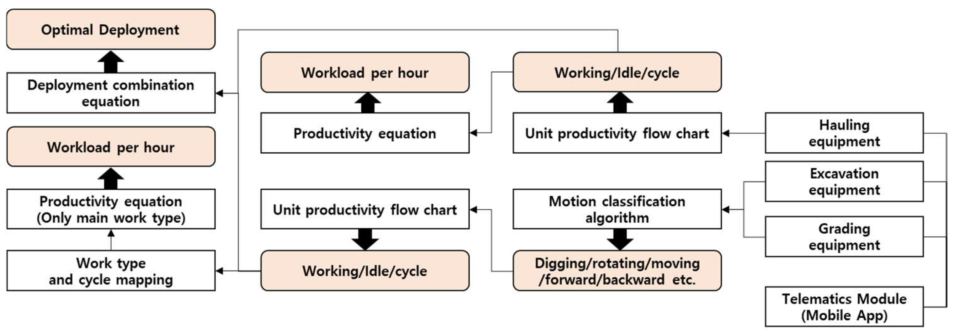
The Earthwork Unit Productivity Module gathers information of the earthwork equipment to classify the motion using system data processing methods based on algorithms developed for each of the earthwork equipment. Equipment, such as excavators and dozers, are capable of identifying movements like rotation, digging/loading, forward and backward motion, and stopping, utilizing self-developed motion analysis algorithms. Subsequent to the identification of these movements, each operation is categorized into either work time or rest time. Operations aligned with work time are further grouped into loading cycle, transport cycle, and stop cycle. The motions of the excavators are classified into five categories: digging/loading, rotating, leveling, moving, and stopping. Similarly, to classify the motions of dozers, they are divided into three categories: forward, backward, and stop. The motion classification algorithm was developed to process the data and to classify the motions. The results of the motion classification algorithm are in the Machine Learning Module for work type classification. Based on the above-processed information, the Productivity Module calculates the productivity and deployment combination of the earthwork equipment in real time. Productivity is analyzed in real time by applying the cycle pertinent to the principal work type, along with the specification information of the construction equipment, work time, and rest time into the productivity calculation formula.
Additionally, the recommended number of dump trucks is computed as a planning-level fleet-sizing indicator based on the excavator efficiency and GNSS-observed cycle times. The system data processing workflow is shown in Figure 2. Within this framework, ‘e-fleet management’ (web-based platform) and ‘e-map’ (mobile app) are integral components and are user interfaces allowing for the interaction of information to project managers in visual representation, with the ‘e’ denoting ‘earthworks’. It processes construction equipment data conforming to the NMEA 0183 protocol and to mobile information from the e-map. A database stores all the information, and the BIM–GIS Module provides the information in terms of orthophoto maps, point clouds, CAD, and geofencing areas.

3.2. Platform Structure

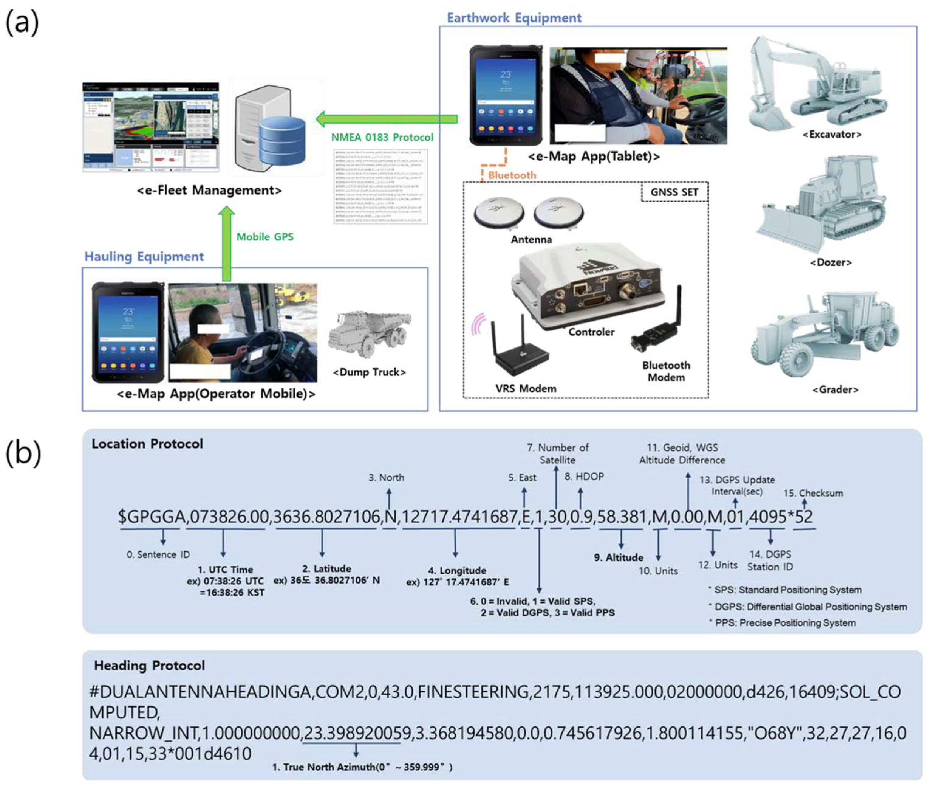
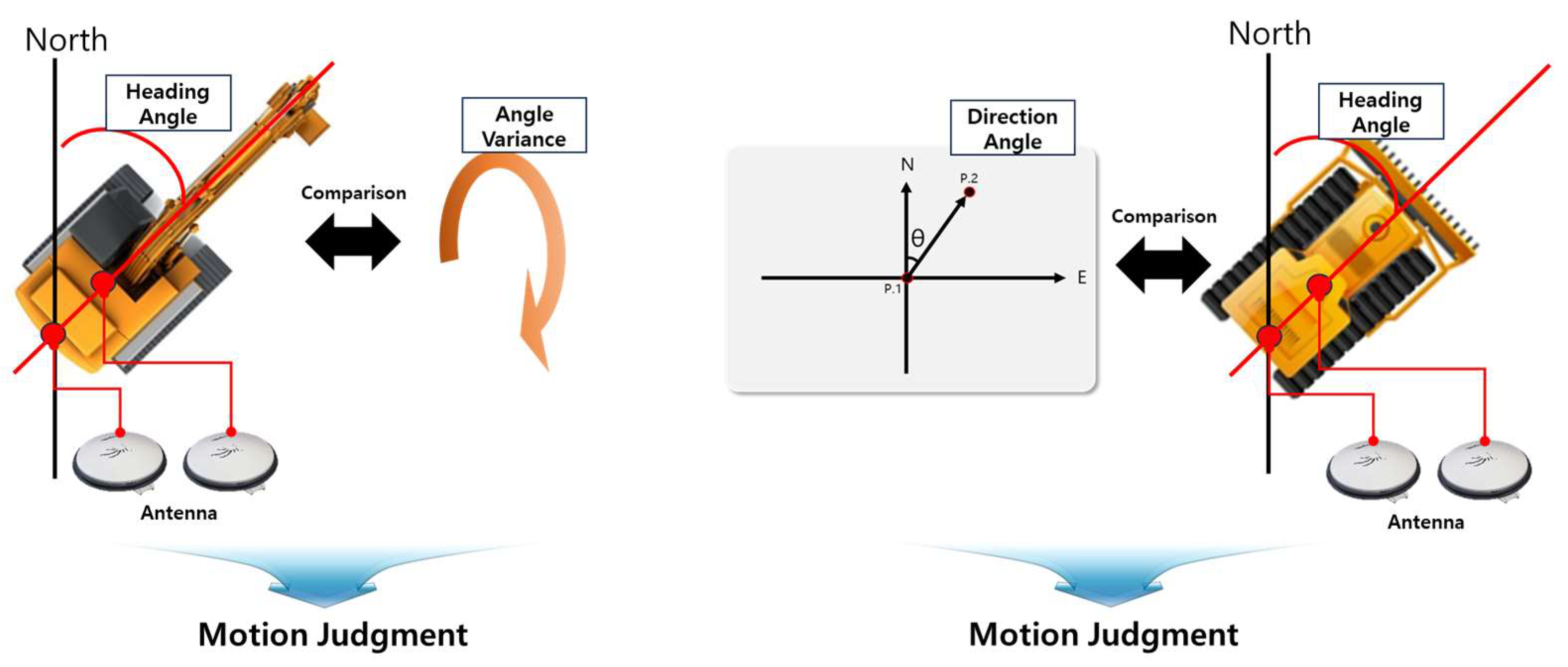
The platform structure gathers the information from the earthwork machines, GNSS, and mobile GPS data, and stores the information in the database, which is then processed based on the developed algorithms and the productivity report is generated. Figure 3a represents the configuration of the e-map. In general, excavators, dozers, and graders are set up using high-precision GPS equipment and onboard tablets. For dump trucks, the system is established by installing the e-map application on the driver’s mobile phone. Most local earthwork companies do not assign specific dump trucks for the project but rather dispatch them on a daily basis. Therefore, the installation method on mobile phones was adopted considering the practicality of dump truck operations. Figure 3b depicts the protocol generated by the e-map. The key aspects of the protocol include latitude, longitude, altitude, heading, and quality information based on coordinated universal time (UTC). When the quality information is transmitted as 0, the data are excluded from algorithmic analysis and other processes on the e-fleet management server. Figure 4 depicts the GPS equipment installation method and criteria for the e-map. The equipment’s alignment with true north is used to determine the angle change. The excavator primarily uses GPS angle changes for motion classification, while graders depend on the angle difference between the GPS and direction.
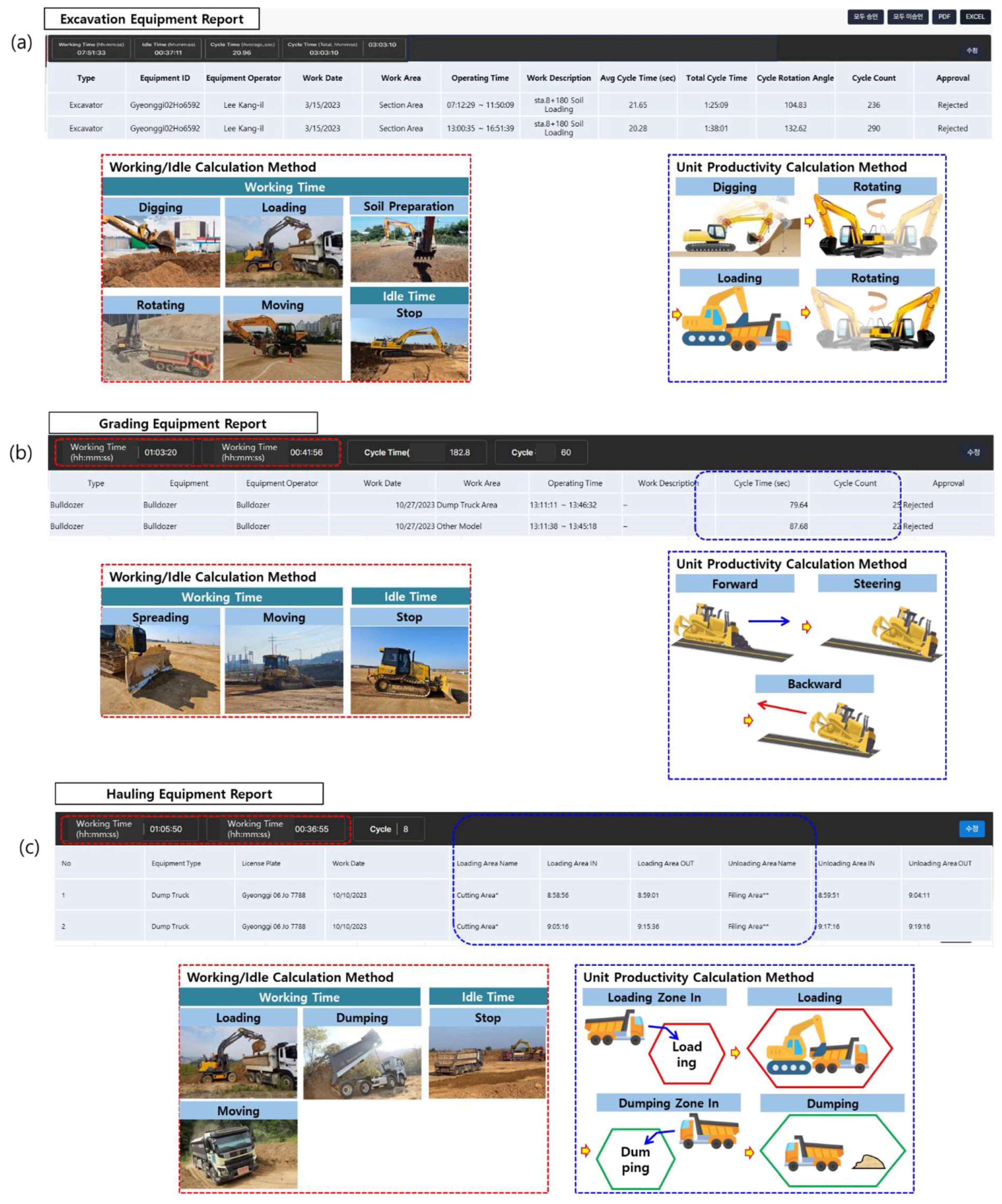
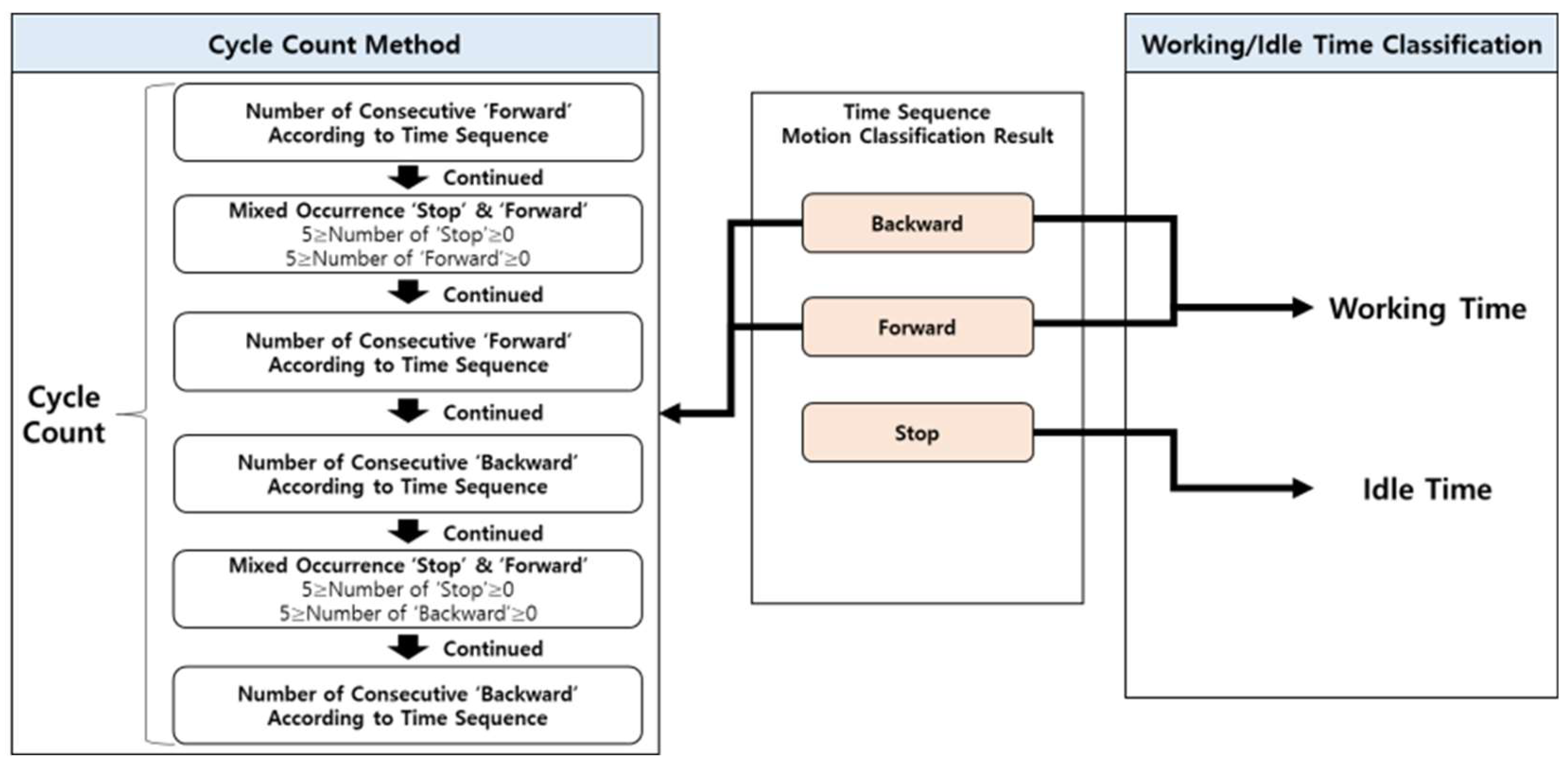
The concept of a unit productivity report for excavation equipment is illustrated in Figure 5a. Working time and idle time are categorized based on activities such as digging/loading, stopping, rotating, moving, and soil preparation. Soil preparation refers to fine leveling/position adjustment operations in which the machine may exhibit small heading changes while remaining nearly stationary. At very low speeds, the GNSS-derived heading can fluctuate; therefore, brief soil preparation segments may be intermittently labeled as a stop under noisy heading conditions. Motion classification algorithms determine the criteria for categorizing these activities, which define a single cycle as digging, rotating, loading, and rotating again. Figure 5b shows a unit productivity report for the grading equipment. Unlike the excavation equipment, working time and idle time are categorized based on activities such as stop, forward, and backward. Motion classification algorithms are employed to establish the criteria for classifying activities as stop, forward, and backward. A single cycle is defined as forwards to stop to backwards or forwards to backwards. Figure 5c shows a unit productivity report for the hauling equipment. Working and idle time are calculated based on the displacement of over or under 0.5 m. A single cycle is defined as entering the loading zone and exiting from the dumping.

3.3. Fleet Telematics System Algorithms

3.3.1. Hauling Equipment Productivity

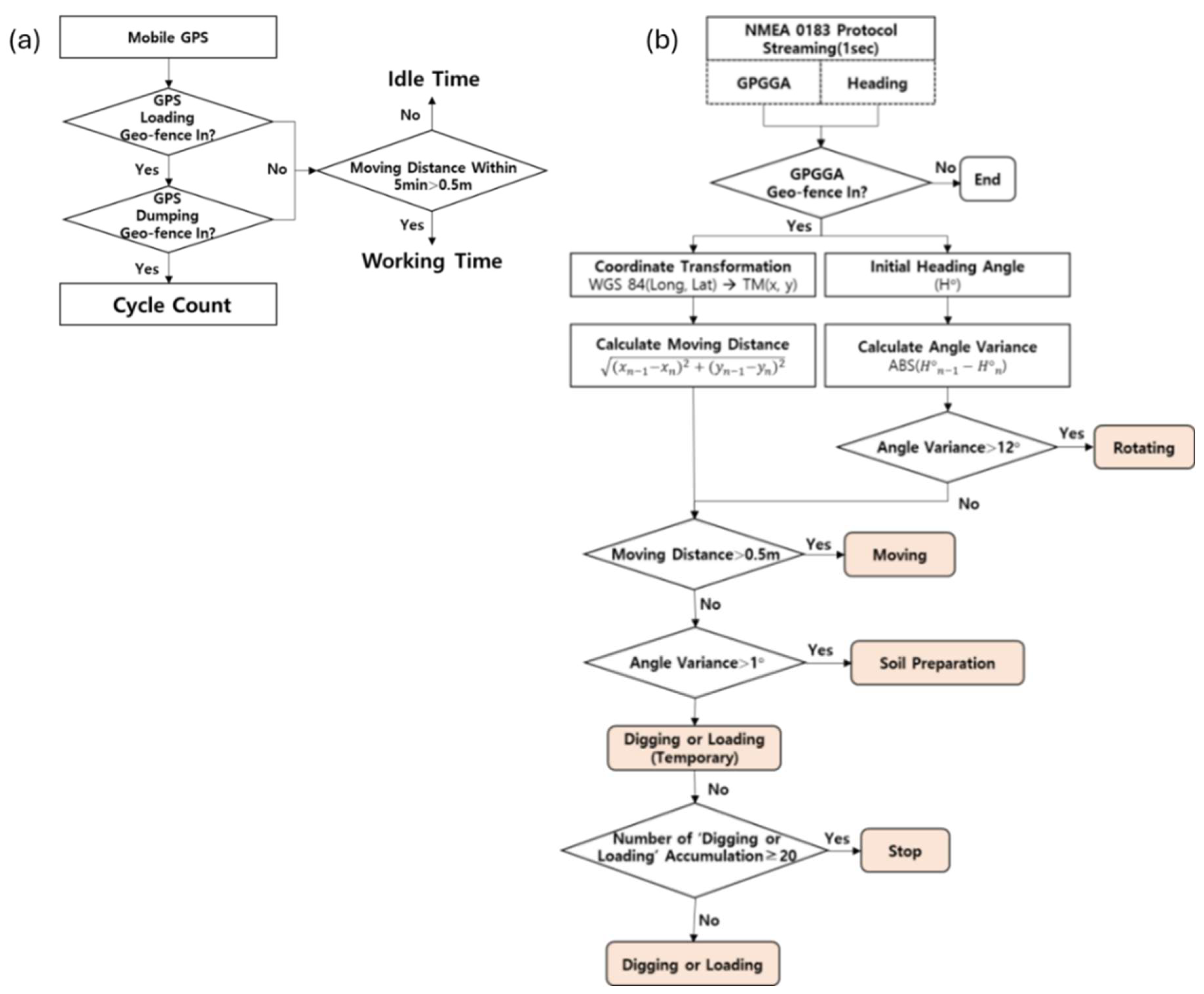
For the dump productivity calculation, the ray casting algorithm is used to determine the number of dump truck cycles. The ray casting algorithm, also known as the crossing number or even–odd rule algorithm, has been known since 1962 [46]. It tests the number of times a ray intersects its edges to determine whether a certain point lies inside or outside a simple polygon. The ray can start from any point and move in any fixed direction. If the point is outside the polygon, the ray will intersect the polygon edges an even number of times. Conversely, if the point is inside the polygon, the polygon edges will be intersected an odd number of times. The ray casting algorithm determines the in/out status of the hauling equipment in the geofence area. It assigns attribute information to the geofence to distinguish between loading and unloading points. Geofences and loading/unloading/work areas are defined by the site manager within the e-Fleet Management BIM–GIS interface (or imported from existing CAD/GIS layers) and can be updated whenever the site layout changes. For highly dynamic sites where loading/dumping locations change frequently, the geofence polygons can be rapidly updated in the BIM–GIS interface, and the Cycle Detection Module uses the updated geofences for the subsequent cycle computation. The cycle calculation is then based on the in/out status of the loading and unloading points. If the hauling equipment remains motionless for more than 5 min with no movement exceeding 0.5 m without entering the loading or unloading geofence, it is classified as idle time; otherwise, it is classified as working time (Figure 6a). Refer to Section 3.3.2 for a detailed explanation of Figure 6b.
The calculated number of cycles is used in Equation (1) to perform a productivity analysis for the hauling equipment. The productivity analysis refers to the amount of work performed per hour. The number of cycles can be considered as the number of hauling trips. The hauling productivity is calculated by multiplying the number of trips by the loading capacity of the hauling equipment and the volume of the earthwork, and then dividing this by the total time required. The total number of cycles (i.e., hauling trips) is then used to compute the unit productivity using Equation (1) as follows:
P i = i V i T c , i
where
P i = productivity of equipment i (m3/h);
V i = total volume of material handled by equipment i (m3); that is (No. of Cycles × Load Volume)
T c , i = total cycle time of equipment i (h); that is (Working Time + Idle Time)
Equation (1) is used as a baseline productivity definition driven by GNSS-derived cycle segmentation; it is not intended as a stochastic hauling model. Because cycle timestamps are obtained from 1 Hz GNSS geofence crossings, the resulting cycle times include a bounded timing uncertainty at the scale of seconds (see feasibility verification in Table 4), and productivity is therefore interpreted as the aggregation-window level rather than as the second-level ground truth.

3.3.2. Excavation Equipment Motion Classification and Productivity

The motion analysis algorithm used for the excavation equipment is illustrated in Figure 6b. It begins upon receiving the data from the e-map protocol defined in e-fleet management to determine the entry status of the excavator in the geofence. The geofence represents the user-defined work area for the excavation equipment. The algorithm’s analysis is based on the location information (x, y) and the heading information (angle) to decide whether the equipment enters the defined work area. The distance between two points is calculated using location information, and the angle change is determined by means of heading information.
The movement of the excavation equipment is assessed in three stages. First, if the angle change is greater than 12°, it is classified as rotating. Second, if the angle change is less than 12°, but the displacement is greater than 0.5 m, it is categorized as moving. Third, if the angle change is greater than 1°, it is classified as soil preparation. If the angle change is less than 1°, but the excavator is digging or loading, an additional filtering step is applied, named as a stop, which means it is idle. If digging or loading activities accumulate for more than or equal to 20 s, all digging or loading activity data from the previous 20 s are considered a stop. After conducting mock tests with two excavators with different bucket specifications. The rotating parameter was tested to find the most suitable value considering the excavator movements, and it was found to be 12°. Decreasing the angle change value parameter below 12° classifies minor movements as rotating, leading to an overestimated cycle count. The moving parameter was determined based on the equipment’s minimum speed. Meanwhile, the soil preparation parameter was established to detect minor movements and to classify them as any other activity than rotation. This parameter addresses the limitations of GPS sensors, which cannot detect the movement of the excavator’s boom, arm, and bucket. A 20-s time buffer was implemented to assess digging or loading.
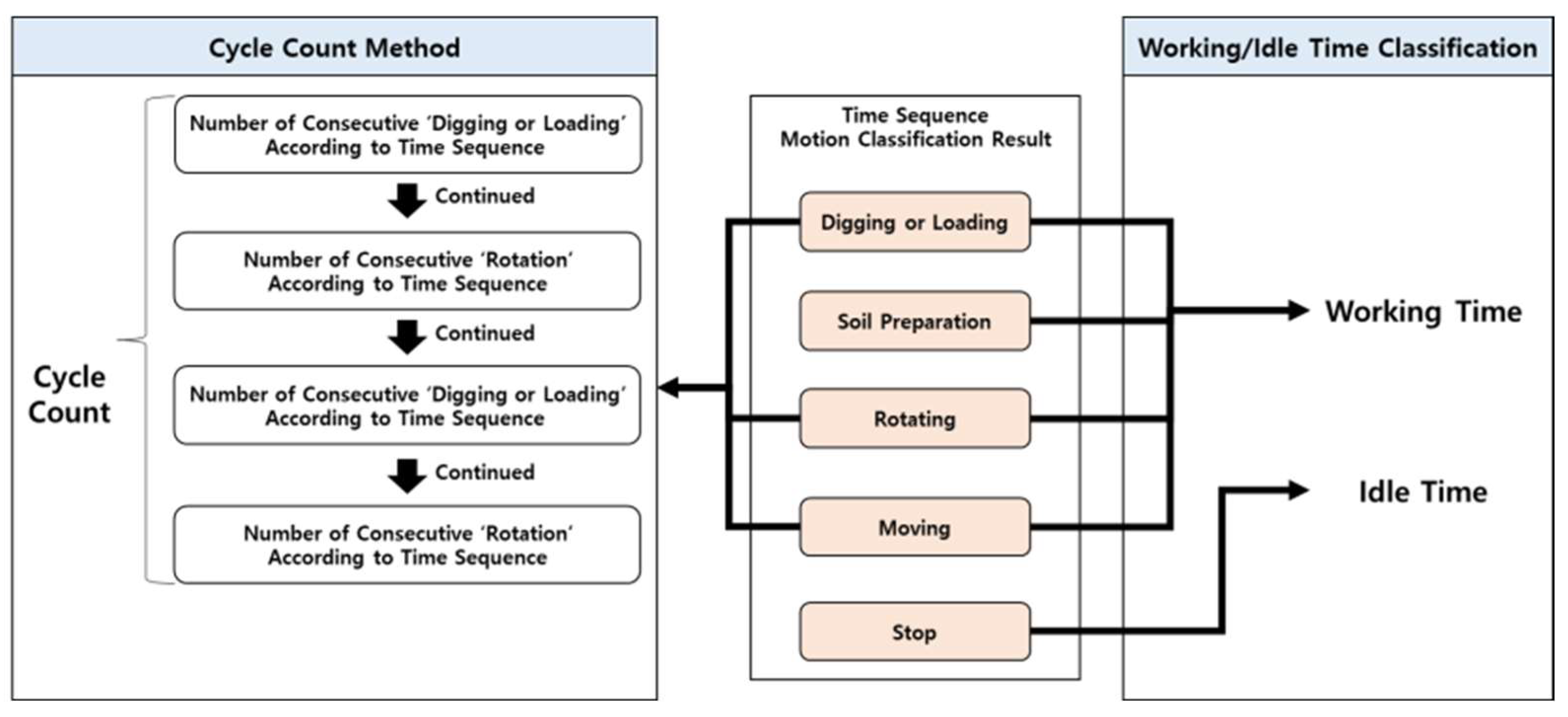
The number of cycles, working time, and idle time for the excavation equipment are determined based on the classified motion shown in Figure 7. Digging/loading, rotating, moving, and soil preparation activities are classified as working time, while a stop is considered idle time. If digging/loading, rotating, moving, and soil preparation occur continuously in a sequence without interruption, it is considered a single cycle. The number of cycles computed is used in Equation (2) to analyze productivity for the excavation equipment. Productivity refers to the amount of work completed in a given time, similar to the hauling equipment.
P e x c = N c y c l e × V b u c k e t T w o r k + T i d l e
where
P e x c = productivity of the excavator (m3/h);
N c y c l e = number of excavation cycles (–);
V b u c k e t = bucket volume (m3);
T w o r k = total working time (h);
T i d l e = total idle time (h).
In Equation (2), V bucket is treated as an effective operating capacity (nominal capacity × field fill factor) when reporting real site productivity. Accordingly, we present nominal estimates for initialization and then verify/calibrate the effective capacities using independent drone-based volume measurements.

3.3.3. Grading Equipment Motion Classification and Productivity

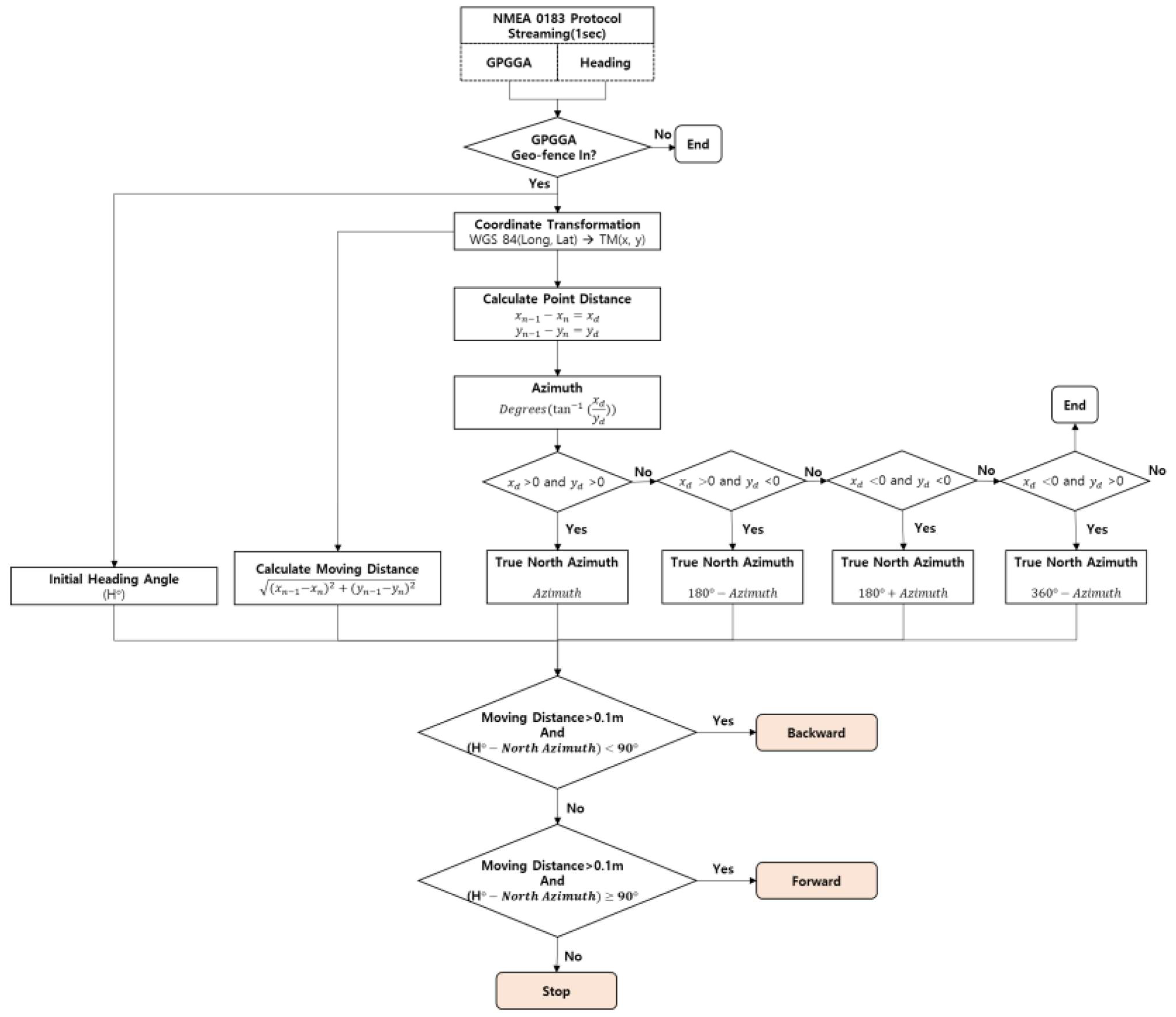
The motion analysis algorithm for grading equipment, as shown in Figure 8, is similar to that of the excavation equipment. Upon receiving the e-map protocol in e-fleet management, it determines whether the equipment has entered the geofence project area. It calculates the distance between two points in terms of x and y coordinates and uses this information to determine the true north azimuth. Simultaneously, it computes the displacement during movement. Using the true north azimuth, the GPS heading, and the displacement, the algorithm first identifies the backward movement. If the difference between the GPS heading and the true north azimuth is less than 90° and the displacement is greater than 0.1 m, it is classified as backward movement. If the difference is greater than or equal to 90° and the displacement is greater than 0.1 m, it is classified as forward movement. If the location information shows a displacement of 0.1 m or less, it is considered to be idle, named as a stop in the algorithm. The forward and backward movement algorithm was developed to address cases where the equipment’s direction and heading data are reversed. If the forward and backward parameters are excessively large compared to 90°, it may be difficult to distinguish between changes in the two parameters. Conversely, if they are excessively small, it may lead to erratic forward and backward detections due to errors in the GPS data.
The workflow to calculate the number of cycles, working time, and idle time for the grading equipment based on classified motions is shown in Figure 9. Generally, forward and backward movement is categorized as working time, while a stop is categorized as idle time. Both forward to backward, forward movement to a stop, and then move backwards are considered one single cycle. In situations where the grader stops moving and then starts again, any forward, stop, and backward activity, and if the equipment is idle for less than 5 s, it will be considered part of a single cycle and will not be counted as a stop.

3.3.4. Planning-Level Recommended Equipment Combination

Previous studies have not focused on determining the optimal equipment deployment combinations based on real-time productivity analysis for earthwork operations. This study identifies the most recommended equipment combination for earthwork operations by analyzing the productivity of the excavators and determining the maximum number of dump trucks required through several equations. The first dump truck shift time is determined from actual earthwork operations. Then, the number of excavator cycles per dump truck is calculated using Equation (3). The next step is determining the time the excavator requires to complete loading one dump truck using Equation (4).
N e x c / d t = N e x c _ c y c l e N d t _ c y c l e
where
N e x c / d t = number of excavator cycles per dump truck (-);
N e x c _ c y c l e = total number of excavator cycles (-);
N d t _ c y c l e = total number of dump truck cycles (-).
T l o a d , e x c = T l o a d , e x c _ s i n g l e × N e x c / d t
where
T l o a d , e x c = total excavator loading time per dump truck (s);
T l o a d , e x c _ s i n g l e = time required for one excavator loading operation (s).
It is important to calculate the number of dump truck hauls when the excavator is operating at maximum efficiency. The time required for the existing dump truck to leave and another dump truck to enter in the reverse direction once the excavator has completed loading must also be considered. Therefore, Equation (5) is used to determine the number of dump truck cycles at the excavator’s maximum working capacity. It considers the time required for the excavator to load one dump truck from Equation (4) and the shift time for each dump truck yields the absolute time required for the excavator to accommodate one dump truck. Then, using Equation (6), the number of cycles for one truck is calculated. Finally, the recommended equipment combination of a total number of dump trucks according to the excavator’s maximum working capacity is determined using Equation (7).
N d t , m a x = T w o r k + T i d l e T s h i f t , d t + T l o a d , e x c
where
N d t , m a x = number of dump truck cycles at the excavator’s maximum working capacity (-);
T w o r k = total working time of the excavator (s);
T i d l e = idle time (s);
T s h i f t , d t = shift time of a dump truck (s);
N d t , o n e = N d t , m a x N d t , t o t a l
where
N d t , o n e = number of cycles per single dump truck (-);
N d t , t o t a l = total number of dump trucks in operation (-).
C o p t = N d t , m a x N d t , o n e
where
C o p t = recommended equipment combination (planning-level) (-);
Equation (7) provides a recommended number of dump trucks to balance the excavator loading capacity and the dump truck cycle time under steady-cycle, average-cycle, assumptions, using average loading time, and average haul-cycle time. The formulation assumes approximately constant operating conditions within the selected analysis window and does not explicitly model stochastic disruptions (e.g., traffic congestion, route variability, mechanical breakdowns, or queuing). Therefore, the result should be interpreted as a practical planning guideline rather than a stochastic scheduling optimum.

4. Evaluation and Feasibility Validation

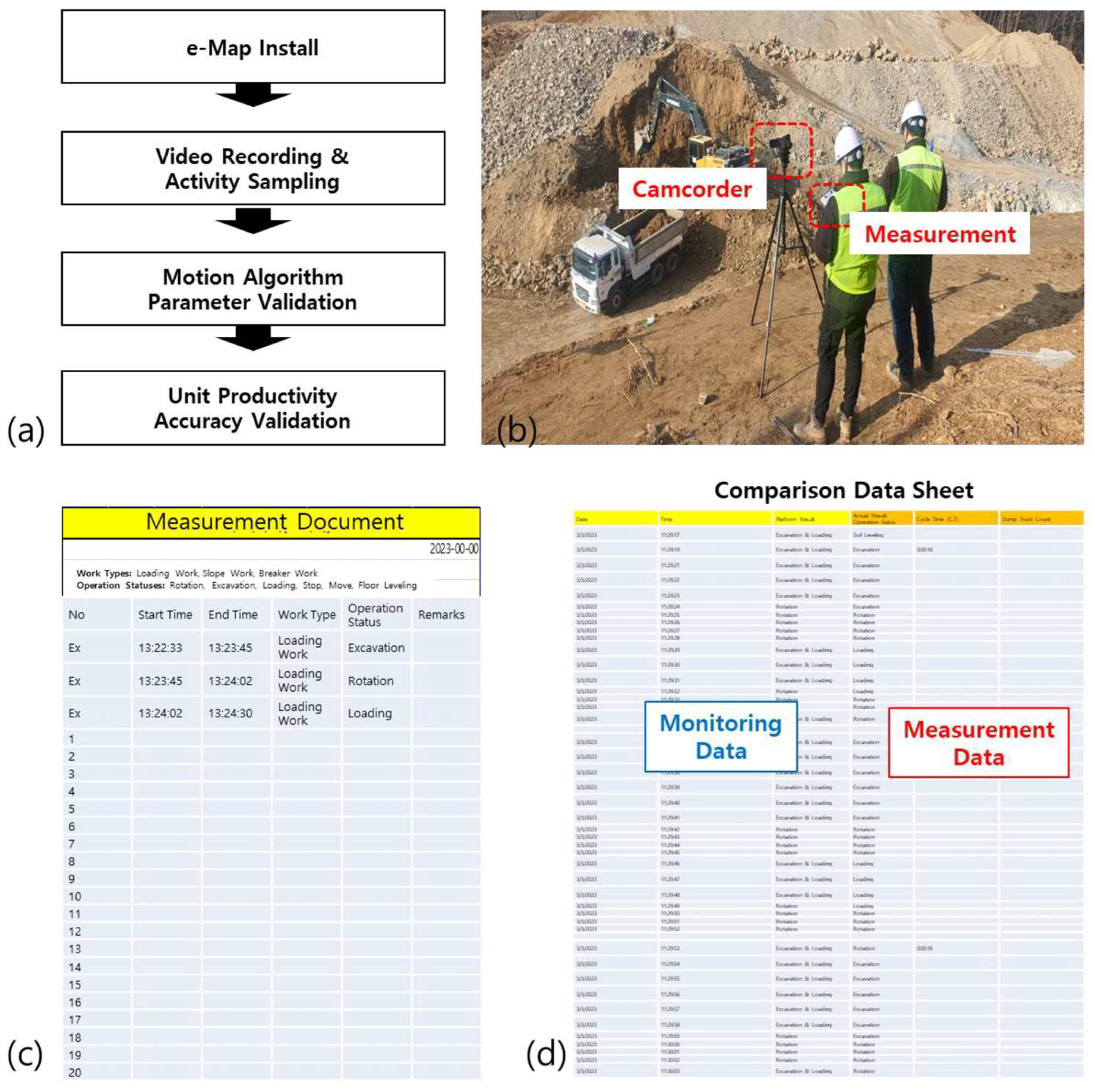
The evaluation and validation were performed from three aspects: the validation of motion algorithm, parameter accuracy, and unit productivity accuracy. This process compares the results of the developed intelligent fleet monitoring technology with actual field measurements at the earthwork site. Figure 10a shows the evaluation and validation process. A mobile app was deployed on all types of earthwork equipment along with a camcorder recording at the same time to record actual equipment operations (Figure 10b). Camcorder recording was carried out to record the actions of the actual equipment down to the second, and it was performed with precision to enhance accuracy. Camcorders were set up around the excavators and dozers to record the operations of both the excavators and the dozers, as well as the dump trucks approaching the respective equipment. Manual activity labels (ground truth) were obtained by reviewing the synchronized camcorder videos using predefined start/end rules for each activity and time-stamping at 1 s resolution. Manual labeling can involve subjective judgment; inter-observer variability was not quantified in the current dataset and was acknowledged to be a limitation. The activities of the excavator and the loader were defined from the literature [4]. Figure 10c shows the site document intended for the recording equipment operations. Figure 10d exhibits the document that compares the algorithmic results derived from e-fleet management with actual measured results by time-matching to validate the practicality; a comparison analysis of the actual measurement data and the information displayed on the developed platform was conducted. The results of the motion algorithm are analyzed, and a comparative analysis of the unit productivity information, such as cycle time, number of cycles, and idle time, is performed with the actual measurement data.

4.1. Calculation Basis for Motion Algorithm ‘Stop’ and ‘Rotating’ Parameter

Table 2 presents the validation test details for a stop motion. The equipment’s per-second travel distance was measured based on RPM, and the measurement continued for 6 min and 43 s. The measurement results showed that, at low RPM, the per-second forward and reverse travel distances were 0.77 m; while, at high RPM, they were 0.92 m. Considering the possibility of a rapid reduction in travel distance just before the actual stop of the equipment and taking into account the test results, the algorithm of this system was designed to classify it as a stop motion when the movement is less than 0.5 m per second.
As shown in Table 2, the per-second travel distance under low/high RPM exhibits a small dispersion (SD = 0.017 m) with a tight 95% CI (0.75–0.79 m for low RPM and 0.90–0.94 m for high RPM), indicating repeatable measurements under steady motion. Therefore, a stop threshold of 0.5 m/s was set conservatively below the lower CI bound to accommodate deceleration immediately before a full stop and potential GNSS-induced fluctuations.
To quantify the variability and robustness of the empirical parameters, we report the standard deviation (SD) and the 95% confidence interval (CI) of the mean for each indicator. The 95% CI was computed as x ¯ ± t 0.975 , n 1 s / n , where n is the number of samples, s is the sample SD, and t denotes the Student’s t critical value. Narrow CIs indicate stable measurements across repeated trials, whereas wider CIs reflect operational variability that should be considered when selecting conservative thresholds.
Table 3 presents the validation test details for a rotating motion. Angle changes were measured in two types of operations: loading and excavation, and the measurement was carried out for 7 min and 54 s. The results indicated that the average angle change in loading operations was 23.71°, while in excavation operations, it was 19.21°. Upon examining the minimum angle change, it was found to be 14.21°. Based on this, the algorithm was designed to classify it as a rotating motion if the movement is 12° or more.
Table 3 shows that the mean angular variance during rotating segments is substantially larger than the selected threshold, with 95% CIs of 20.40–27.03° (loading work type) and 14.88–23.54° (slope work type). Since the lower CI bound (14.88°) remains above 12°, the chosen threshold provides a separation margin that is robust to within-class variability.
Table 4 provides the validation test details for the soil preparation motion. This test was conducted for the purpose of classifying data as a soil preparation motion or as a digging/loading motion, excluding a rotating motion. The measurement was conducted for 20 min. The results showed that the average angle change was 5.66°, and the minimum angle change was 1.97°. Based on this, the algorithm was designed to classify it as a soil preparation motion if the movement is 1° or more, and as a digging/loading motion if the movement is 1° or less.
In Table 4, the soil preparation segments show a mean angular variance of 5.66° with a 95% CI of 3.44–7.88°. The threshold of 1° was selected well below the lower CI bound to reliably capture sustained minor posture changes while minimizing missed detections as the soil preparation > 1° and the digging/loading ≤ 1°.
Table 5 provides the validation test details for the digging/loading motion. This test was conducted to classify a stop motion additionally within the digging/loading motion. As the GNSS equipment cannot measure digging/loading motion directly, a time buffer was planned, and the measurement was carried out for 8 min and 31 s. The results showed that both digging and loading required approximately 6.5 s each, while digging required a relatively longer time. Accordingly, to separate short digging/loading stationary events from prolonged stoppages, the algorithm classifies a stationary segment as digging/loading when the duration is ≤20 s, and a stop when the duration exceeds 20 s.
Table 5 indicates the noticeable variability in the observed digging/loading durations (SD = 3.6 s; 95% CI = 4.21–8.79 s), reflecting operational fluctuations that cannot be directly sensed by GNSS. Hence, a time buffer-based criterion was adopted, and the 20 s threshold was intentionally set beyond the typical single digging/loading duration to reduce false segmentation under intermittent pauses and measurement noise.
Table 6 provides the validation test details for forward and reverse motion. This test was conducted to determine forward and reverse motion by calculating the difference between the true north azimuth, based on heading and position values derived from GNSS, and the direction in which the dozer is facing. The measurement was conducted for 35 min and 6 s.
The results indicated that forward motion could be classified when the direction the dozer was facing was 180° opposite to the direction of travel, while reverse motion could be classified when the dozer’s facing direction matched the direction of travel. Due to location information errors (within ±2 cm), it was determined that there could be a difference between the true north azimuth and the heading. Taking this into consideration, the algorithm was designed to classify it as forward motion when the difference between the heading and the true north azimuth is greater than 90° and as reverse motion when it is less than 90°.
Table 6 demonstrates clear separation between forward and backward conditions: the forward angle margin is tightly concentrated around 180° (mean 180.59°, 95% CI 177.32–183.86°), whereas the backward condition is near 0° (mean 5.02°, 95% CI 2.26–7.78°). Therefore, the 90° threshold provides a wide decision margin that is robust to GNSS heading/position uncertainties. In this study, the GNSS position determination antenna was installed on the front of the vehicle for alignment, and the heading determination antenna was installed on the rear. If these antennas are installed in reverse, it may be necessary to reverse the criteria in the parameters accordingly.
In this study, work states were classified using a rule-based approach based on the motion displacements computed from GNSS-derived equipment motions. The threshold values for each rule were determined by comparing the distributions of state-specific indicators in the sample data and selecting boundary values that maximized separability between the states.
Excavator rotating (Rotating): A segment was classified as rotating when the cumulative heading (angular) change over a continuous interval exceeded 12° (>12°).
Equipment moving (Moving): A segment was classified as moving when the planar displacement over a continuous interval exceeded 0.5 m (>0.5 m).
Soil preparation (Soil preparation): To capture intervals characterized by sustained minor posture changes, the angular change threshold was set to greater than 1° (>1°).
Stop vs. Digging/Loading: Because GNSS cannot directly observe digging/loading, stationary segments are differentiated by duration. A segment is classified as digging/loading when the stationary duration is ≤20 s, and as a stop when the stationary duration is >20 s (≤20 s/>20 s).
Forward/Backward: Based on the relative angle of the travel direction vector, motion was classified as forward when the relative angle was ≥90°, and as backward when it was ≤90° (≥90°/≤90°).
These threshold-based rules have the advantage of being GNSS-only, i.e., they do not require auxiliary onboard sensors (e.g., IMU/accelerometers or machine control signals) and instead rely exclusively on the GNSS-derived displacement and heading indicators. In this study, geofence definitions are treated as a lightweight site configuration layer (operational zone labeling) rather than as an additional sensing modality, enabling scalable deployment while preserving a single sensor data stream.
Parameter values were estimated by partially extracting and measuring the GNSS data from the equipment that was actually operated in this case study; therefore, the thresholds should be recalibrated when applying the method to other equipment.
To further address robustness beyond the descriptive statistics, we conducted a local parameter sweep around the candidate thresholds (displacement, angular change, and time buffer values) and quantified the resulting motion classification/proxy productivity errors against manually labeled reference segments. The results show that reducing the thresholds below the selected values increases the false state transitions due to GNSS jitter and heading instability at low speeds, whereas increasing the thresholds leads to missed short operational transitions. The adopted parameter set therefore represents a transparent accuracy–robustness trade-off under the tested GNSS conditions.

4.2. Motion Algorithm Evaluation and Feasibility Validation

A comparative analysis was carried out for the excavators and dozers to optimize the motion algorithms by comparing their actual motion measurements and varying the algorithm parameters. The motion algorithm parameters for the excavator are as follows: an angle change of 12° for rotation, a displacement of over 0.5 m for movement, an angle change of more than 1° for soil preparation, and the stop parameter is 20 s when the excavator remains idle for more than 20 s. A sensitivity analysis was carried out by varying all these parameters, as shown in Table 7. The very large percentage errors in Table 7 occur only under intentionally mis-specified sensitivity settings (e.g., overly small displacement thresholds), which cause over-segmentation due to GNSS jitter and heading instability at low speeds. Because the percentage error can be unstable when the ground truth duration/count of a motion state is small (i.e., rare or short duration states), we interpret extreme percentages in the sensitivity tests primarily as a denominator effect. To improve robustness and interpretability, we report (i) absolute deviations (Δ seconds and Δ counts) alongside percentage errors and (ii) robust summaries (median and interquartile range) across motion states, which are less sensitive to outliers. This dual reporting allows the reader to evaluate the practical impact of parameter changes on productivity-relevant quantities without overstating errors for rare states. Changing the rotating parameter to 15° resulted in a rotational motion error of 12.7% and decreasing this parameter to 10° led to an error of 8.8%. For the analysis of the moving parameters, increasing the parameter to 1 m resulted in an error of 72.2%, while reducing it to 0.1 m caused the motion error to exceed 100%. Testing the soil preparation parameter at 3° results in an error of 77.0%, which is more significant than the 54.1% error compared to an optimal parameter set at 1°. Changing the parameter to 0.5° decreases the error but increases the error in the stop parameter. This error often occurs in the misclassification of stationary equipment motions as soil preparation due to the limitation of GPS, which causes heading errors. Setting the stop parameter to 30 s results in underestimating the stop parameter and overestimating the digging/loading activities. Changing this parameter to 10 s leads to overestimating the stop time and underestimating the digging/loading activities. The motion classification thresholds (e.g., heading change and displacement criteria) were selected to balance (i) GNSS measurement noise and the sampling interval under low-speed earthwork operations and (ii) typical kinematic patterns of excavator/dozer movements. In addition to preliminary mock tests, we quantified the parameter sensitivity using field data (Table 7), showing that overly small thresholds overcount changes while overly large thresholds miss short transitions. The same parameters were further evaluated and set across multiple construction sites with different hauling distances and operational conditions in the case study section.
The grading equipment motion algorithm is based on a determination of the three actions: forward, backward, and stop. After a comparative analysis, the optimal forward/backward parameters were determined to be 90°, and the stop parameters were set to 0.1 m. A sensitivity analysis was performed by varying the parameters to identify the optimal values, as illustrated in Table 8. Changing the forward/backward parameters to 180° results in a motion error of 35.8% and 30.3%, respectively. Conversely, adjusting these parameters to 10° leads to a motion error of up to 14.6%. Testing the stop parameter by setting it at 0.5 m for grading equipment results in an error margin of up to 2.5%, which also decreased the accuracy of forward/backward motion detection. Increasing the stop parameter to 1.0 m demonstrated an error of 8.0%, indicating a proportional rise in error relative to the results obtained with the 0.5 m parameter test. A sensitivity analysis of the excavation and grading equipment highlights the importance of precise parameter settings for accurately capturing and classifying the various movements of the excavator and grader.

4.3. Unit Productivity Evaluation and Feasibility Validation

The unit productivity of hauling, excavation, and grading equipment is evaluated by comparing the actual measurement of the variables required for unit productivity calculation from the real-time construction project with the results of the development of the Intelligent Fleet Monitoring Technology. For the hauling equipment, entry, exit, total time, and the number of cycles are compared for validation. The actual measurements are recorded using the existing traditional manual system, and the developed system calculates the entry and exit time stamps based on the entry and exit of the hauling equipment in the geofence area (Table 9). The analysis shows an average delay of around 7 s in recording the entry time into the geofence compared to the actual entry time. Similarly, an average delay of approximately 10 s was observed in recording the exit time from the geofence in relation to the actual exit time. However, the number of cycles determined is exactly the same, which is the key variable in determining unit productivity. For completeness, we also report the corresponding absolute time error (seconds) and robust summaries (median and interquartile range) of the entry/exit time offsets, in addition to percentage error, to ensure interpretability even when the true values are short in duration. These values are reported to transparently characterize the timing uncertainty in a geofence-based cycle segmentation at 1 Hz sampling; accordingly, subsequent productivity estimates are presented as practical monitoring indicators aggregated over operational windows rather than as precise second-level measurements. The GNSS-derived heading, course-over-ground, is most reliable during motion and can fluctuate under near-zero speed conditions; this limitation is reflected in the discussion of boundary cases, such as soil preparation versus a stop. Therefore, the developed system’s application is considered acceptable for effective and suitable earthwork operations. The analysis highlights the system’s ability to provide reliable data, despite minor time lag discrepancies deemed insignificant for overall productivity analysis.
A unit productivity analysis of the excavation equipment was conducted over two sessions, lasting 44 min and 40 s and 4 h, 18 min, and 35 s, respectively. The results presented in Table 10 indicate that the error for cycle time, total cycle time, number of cycles, and idle time determined by the developed algorithm was less than 2.5% compared to the ground truth values. In addition to the percentage error, absolute deviations (seconds and cycle counts) are provided to avoid overstating the performance when denominators are small and to improve comparability across sites and operating conditions. The results show the system’s validity for earthwork operations, as this amount of error is considered acceptable. A detailed analysis of the data for each activity provided the insight that this error was mainly due to the soil preparation activity, which was misinterpreted as a stop or grouped into one cycle. Consequently, this results in errors in the cycle information and idle time. This is due to the highly irregular movement of excavators during soil preparation, and its fundamental operation overlaps with all other activities as well. The analysis emphasizes the system’s capability in accurately determining and analyzing the operations of excavators, thereby confirming its appropriateness for deployment in real-world contexts. The data from the motion accuracy analysis of the grading equipment was used to analyze the average cycle time, total cycle time, number of cycles, and idle time to validate the unit productivity algorithm. The results are shown in Table 10. It clearly indicates that the error was less than 1.3% for all the variables required for the unit productivity calculations. The detailed analysis of each motion activity identifies that there were some cases where minor movements just before coming to a stop or during the transition from forward to reverse were classified as a stop. Also, vibrations from the chassis frame resulted in a stop motion being interpreted as forward and reverse movements. The total number of cycles, which is a key parameter for productivity calculation, is identified correctly. This level of precision is considered satisfactory for grading earthwork operations. It endorses the system’s accurate assessment of earthwork productivity measurement in real-world construction environments for the decision-making process. The unit productivity evaluation and feasibility validation of the developed system shows that it is effective in accurately identifying and analyzing tasks performed by different earthwork equipment.

5. Practical Implementation and Case Study

5.1. Case Study Overview

A case study was conducted at two construction sites for the practical implementation of the developed intelligent fleet monitoring technology for productivity management of the earthwork equipment. The developed system was implemented from March to April at the Pocheon Road Construction Project and in June and from August to October at the Yeongjong Road Construction Project for this case study. Using the proposed intelligent fleet monitoring system, various construction equipment, including a Hyundai 1.5 m3 excavator, a Komatsu 2.0 m3 excavator, a Doosan 1.5 m3 excavator, four 25-ton dump trucks, and one Cat d1 dozer were used at the construction sites. The Hyundai excavator used at the Pocheon Road Construction Project had a dumping zone over 15 Km away. On the other hand, the Komatsu and Doosan excavators, along with the Cat d1 dozer, were employed in the Yeongjong Road Construction Project, where the dumping zone was just 1 Km away. Each of the construction equipment in the fleet monitoring system was equipped with a GPS sensor to enhance the spatial resolution of the equipment at the construction site. The GPS sensor facilitated a real-time analysis of the construction equipment productivity, enabling immediate tracking of progress and efficiency improvements for each of the equipment. Furthermore, the optimal number of dump trucks based on the excavator’s work efficiency was evaluated to assist site managers in planning the equipment deployment combinations. A comparative study was conducted using the dump trucks deployed at the construction site. A device sharing the GPS sensor protocol was also developed for the Doosan 1.5 m3 excavator equipped with Trimble machine guidance. This setup provided a foundation for exploring the potential of integrating the machine guidance systems with the monitoring system in future operations. Importantly, in this study, only the GNSS protocol stream was used for activity classification and productivity computation; the machine guidance internal states were not accessed and a foundation for future integration of the machine guidance internal kinematic states. To examine robustness beyond a single setting, the proposed motion classification and productivity pipeline was applied to multiple excavator models (Hyundai, Komatsu, and Doosan) and to two sites with substantially different hauling distances, approximately 1 km versus > 15 km. While this supports the general applicability of the default parameter set, we note that sites with a markedly different GNSS quality (e.g., severe multipath) or sampling configurations may require minor threshold recalibration, consistent with the sensitivity trends reported in Table 6.

5.2. Equipment Productivity Analysis Using Fleet Telematics System

5.2.1. Unit Productivity

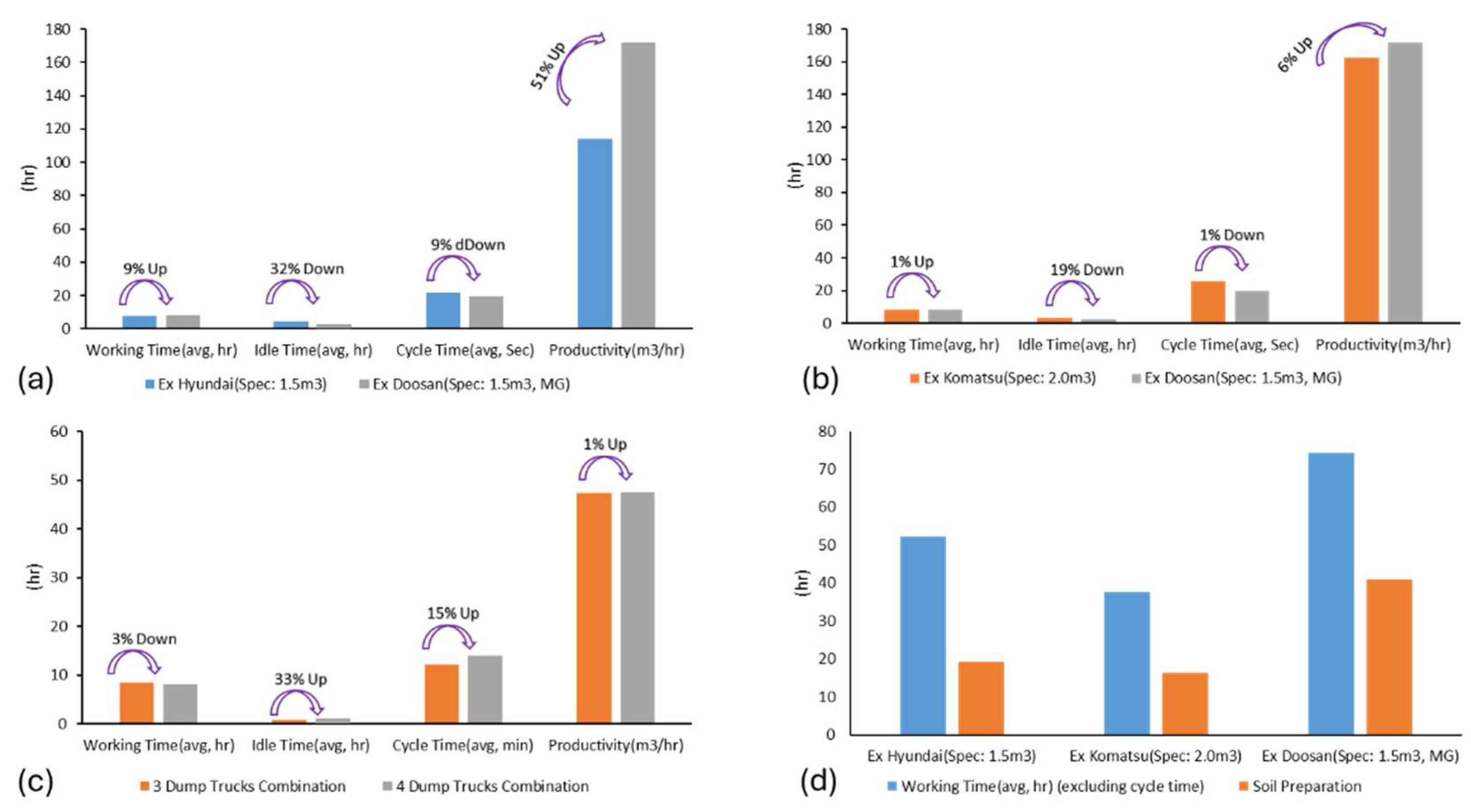
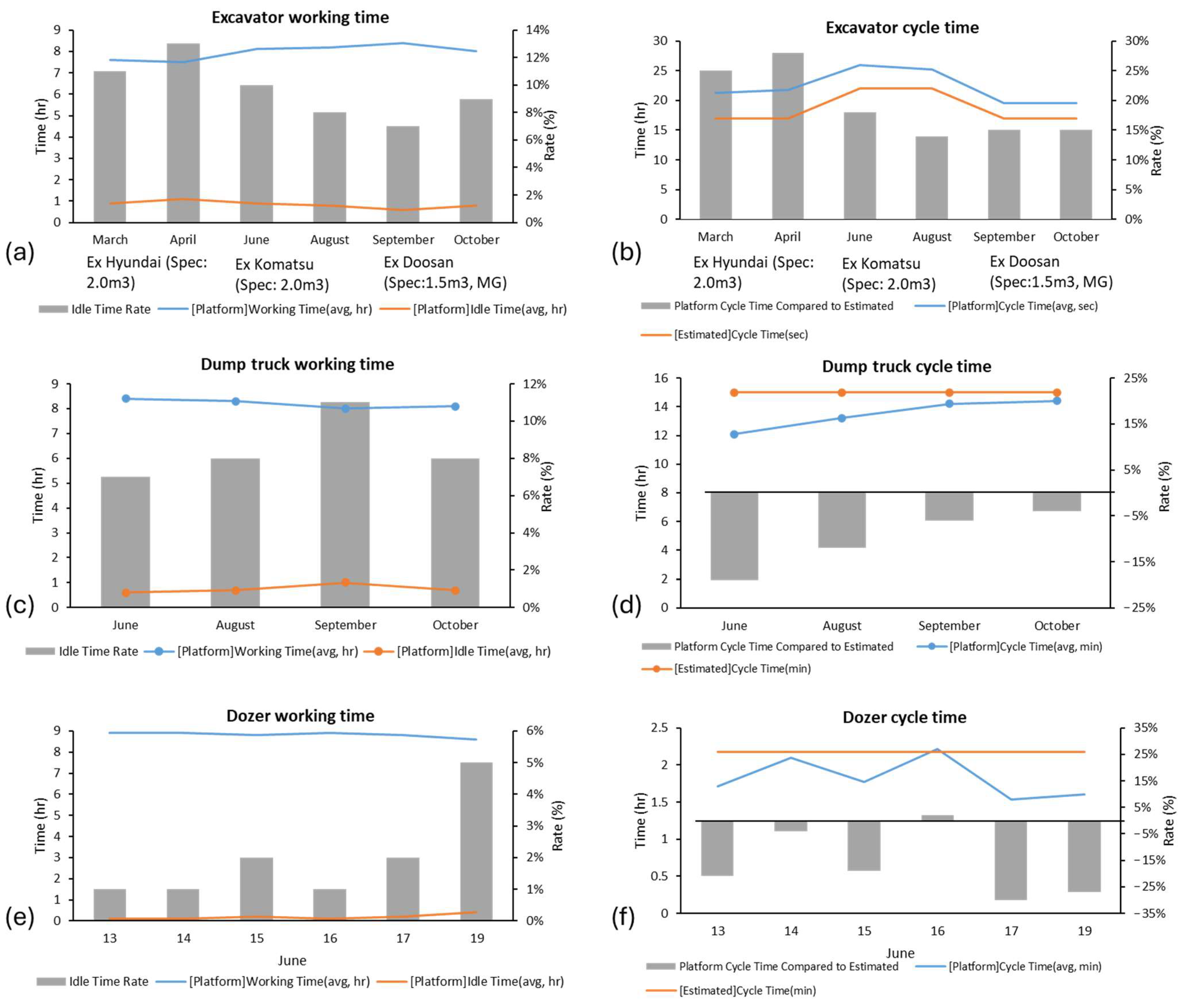
A detailed analysis of the excavators’ working and idle times as evaluated on the platform is shown in Figure 11a. The Hyundai excavator shows the highest percentage of idle time relative to the working hours compared to the Komatsu and Doosan excavators, indicating extended periods of idleness, particularly during loading operations where dump trucks are queuing for the excavator to the load. Therefore, the Hyundai excavator demonstrates a lower cycle time efficiency than the Doosan excavator with similar specifications, suggesting a more efficient dumping cycle and operational environment for the Doosan excavator, as shown in Figure 11b. The Komatsu excavators exhibit a lower cycle efficiency than the Hyundai and Doosan excavators, indicating a lowered working performance at construction sites. Furthermore, the cycle time efficiency compared to the estimated standard was on the lower side for all excavators when compared against the estimated standard. The Doosan excavator showed efficiency metrics closer to the estimated standard, concurrent with a lower idle time proportion and site-specific operating conditions observed during the monitored periods (Figure 11a,b). Because operator strategy and machine-guidance usage were not controlled and the machine guidance internal states were not accessed in the computation, these factors are treated as potential confounders rather than causal drivers. The mean values of the dump trucks’ working and idle times at the Yeongjong–Cheongna site were estimated, as presented in Figure 11c. The discrepancy in the idle time reported during September was due to the prolonged waiting time for dump trucks and delays due to the rolling operation. A gradual decrease in the cycle time efficiency of the dump truck was recorded over successive months, as shown in Figure 11d. The dumping and loading areas were located nearby; it is hypothesized that the overall cycle time efficiency remains comparatively on the higher side when compared to the calculated standard value. An optimal operational route was identified during the dumping operations stages. It can be updated based on system feedback to improve cycle time efficiency in case of changes at the earthwork site. The working and idle time of the dozer for compaction operation for spreading the soil was analyzed daily during the shorter work period at the construction site, as shown in Figure 11e. The cycle time efficiency of the dozers aligns with the estimated standard values, as shown in Figure 11f. However, the cycle time efficiency on 16 June was recorded as a 2% longer cycle time, which is 2 s more than the estimated standard values. It was due to the track compaction operations where forward and backward distances are at the driver’s judgment.

5.2.2. Work Volume

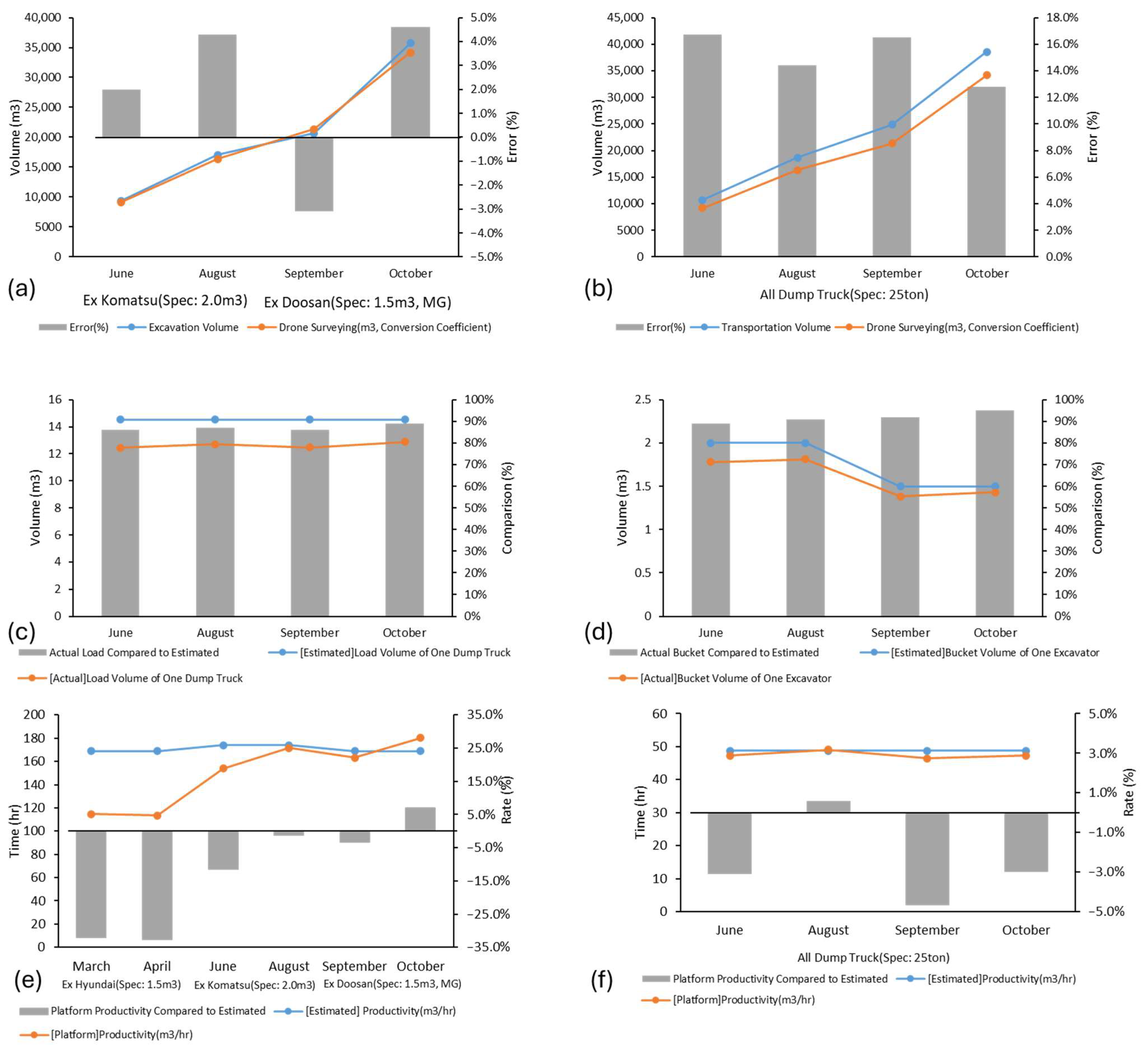
The initial work volume estimation for the excavators and dump trucks was obtained by multiplying the respective load capacities by the number of operational cycles. These preliminary estimations were compared with the volume obtained from drone surveys for a comparative analysis. The comparison based on the drone survey data indicated a volume discrepancy of up to 4.6% for the excavators and 16.7% for the dump trucks, as shown in Figure 12a,b, respectively. Consequently, the 4.6% and 16.7% significant margins of error highlighted the necessity of reevaluation and recalibration of the equipment specifications for excavators and dump trucks. Reevaluation and recalibration ensure that the load capacities accurately reflect real-world working conditions. Figure 12c,d shows the refined outcomes of the excavators’ and dump trucks’ load capacities for enhanced accuracy in the productivity analysis. The initial load capacity of a dump truck was calculated by dividing its cycle count by the results from the drone survey. To find the actual operating bucket capacity for the excavators, the cycle count of a dump truck was divided by its actual load capacity. The calculations showed that the dump trucks’ actual loading capacity was between 12.44 and 12.87 cubic meters. For the Komatsu excavators, the bucket capacity was between 1.78 and 1.81 cubic meters, while for the Doosan excavators, it ranged from 1.38 to 1.43 cubic meters. It was observed that all the target equipment operated with lower excavation and transportation volumes than estimated. This calibration does not modify the productivity formulation itself; rather, it ensures that the capacity inputs used in Equation (2) reflect effective field conditions, thereby aligning the analytical definition with the observed operational variability. The resulting volume discrepancy between nominal-based and drone-calibrated estimates remained within ±5%, which is consistent with stakeholder-accepted tolerances and accepted for earthwork volume monitoring [47,48].

5.2.3. Productivity

Figure 12e compares the excavators’ productivity against the estimated standard. The Hyundai excavators exhibited a reduction of up to 32.7%, while the Komatsu excavators showed reductions of 1.3–11.5%, reflecting differences in the GNSS-derived working/idle time composition and the cycle time efficiency across the monitored periods (Figure 11 and Figure 12). The Doosan excavator showed a 3.3% reduction in September and a 6.9% increase in October; this month-to-month variation coincided with changes in the observed idle time patterns and equipment interaction conditions reflected in the platform outputs (Figure 11c) and with the use of the drone-calibrated effective capacities (Figure 12c,d). Because operator behavior, soil/workface conditions, and site logistics were not experimentally controlled and the machine guidance internal states were not used in the computation, these factors are not interpreted in this study and are instead acknowledged as potential confounders. Figure 12f presents the dump truck productivity estimates and the corresponding calibrated load capacity values; monthly variations are discussed in terms of the observed idle time/downtime patterns rather than causal attribution. The productivity of the dump trucks remains consistent monthly and aligns with the estimated standards. The slight reduction in the productivity of the Doosan excavator during September was due to the soil compaction work and quality testing resulting in the excessive downtime of dump trucks, as depicted in Figure 11c, and indicates potential impacts on the productivity of the excavators, as demonstrated in Figure 12e. This highlights the importance of categorizing different types of work when assessing productivity.
Figure 12. Productivity Analysis: (a) Drone Survey and Excavator Workload Comparison; (b) Drone Survey and Dump Truck Workload Comparison; (c) Actual Load Capacity Calculation of Excavators; (d) Actual Load Capacity Calculation of Dump Trucks; (e) Productivity Analysis for Each Excavator; (f) Productivity Analysis for Dump Trucks.
Applsci 16 01115 g012
Figure 13a illustrates that the Doosan excavators exhibit higher active work time and lower idle time than others in the same category, resulting in superior cycle time efficiency and increased productivity, as indicated in Figure 13b. The results suggest efficient operator work habits, effective machine guidance systems, and strategic positioning of dump trucks when considering excavation sequence and loading processes, reducing cycle times and increasing productivity. Figure 13b demonstrates the Komatsu’s and Doosan’s work time, idle time, and productivity comparison outcomes during the excavation periods. The Doosan excavator has higher productivity compared to the Komatsu excavator despite the lower bucket capacity due to the extended working hours, minimal downtime, and faster cycle time.
The results of a comparative analysis focusing on the impact of the number of dump trucks utilized on the overall productivity are shown in Figure 13c. Operating three dump trucks improved unit productivity, marked by prolonged working time and reduced idle time, reflecting efficient cycle time management. Utilizing four trucks showed marginal productivity improvement due to September’s proof of rolling work and quality inspections. However, the consistent use of dump trucks in October at excavation sites increased productivity (Figure 12e,f). Figure 13d shows that the Doosan excavator had the highest working time and soil preparation work, followed by the Komatsu and Hyundai excavators. This observation is supported by Figure 12c, which demonstrates the significant role of soil preparation in enhancing productivity. The process of soil loosening through soil preparation creates more favorable conditions for excavation, increasing the bucket’s working capacity and overall productivity.

5.2.4. Equipment Deployment Combination

Table 11 provides information on the number of dump trucks and the hauling cycle time in combination with an excavator operating at maximum efficiency. The first attribute represents the average time for replacing the dump trucks loading soil in front of the excavator, which was 29 s. The second attribute indicates the number of loading cycles per single dump truck and the cycle time of the excavator in corresponding months using Equation (3). The third attribute is the excavator loading time, which can be calculated by using Equation (4). The fourth attribute represents the optimal transport cycle for the dump trucks determined by Equation (5), which is calculated by dividing the sum of the excavator’s working time and idle time by the sum of the dump truck’s shift time and the excavator’s loading time. The fourth attribute, “Number of Dump Truck Cycles at the Excavator’s Maximum Working Capacity”, assists in evaluating the hauling cycles of the dump trucks when the excavator operates at maximum efficiency. The average number of one dump truck cycle is calculated using Equation (6), shown as the fifth attribute in Table 11. The sixth attribute indicates the optimal number of dump trucks to be used, calculated using Equation (7). Analyzing dump truck deployment and excavator operations shows that adding another dump truck and increasing the number of excavator operations minimizes the idle time on site. However, this strategy raises concerns regarding potential extended waiting periods for dump trucks during loading. It establishes the possibility that an extra excavator may be required for soil preparation tasks for the loading excavator.

5.2.5. Discussion

This case study evaluated the work efficiency and productivity of various types of equipment. It was found that the rolling process was the primary cause of the excessive idle time observed in the dump trucks. It was necessary to develop a classification technique for the dump trucks, excluding them from the analysis when engaged in rolling operations due to their specific work nature. It was noted that the excavator’s productivity is influenced by the application of machine guidance and the optimal combination of dump trucks by analyzing the differences among the productivity of different excavators. This impact was particularly pronounced in the Pocheon–Hwado site, where there was a significant distance between the dumping and loading areas, leading to the irregular number of cycles of dump trucks and, consequently, to the increased excavators’ downtime. The findings highlighted the need to calculate the required dump trucks based on the excavators’ work efficiency. It also revealed that the equipment’s digging and loading capacities were below the estimated established standards, with productivity being constrained mainly by equipment downtime. A correlation was also established between soil preparation and the overall workload. It is also concluded that executing soil preparation tasks aimed at optimizing the working environment for the excavators leads to increased excavation capacity and overall productivity. However, a practical enhancement is to introduce a short persistence window and heading smoothing to reduce spurious switching between stop and soil preparation states under near zero-speed conditions. Table 12 presents a comprehensive indicator derived from this case study. Recent geometry-aware 3D point-cloud learning approaches also demonstrate how perception modules can improve cutting-point localization in unstructured environments, providing a complementary pathway for future integration with earthwork monitoring pipelines [49].

6. Conclusions

This study set out to develop an intelligent fleet monitoring and management system for construction earthwork equipment based on telematics technology. The system uses only satellite navigation for work type classification based on operational data to provide real-time productivity insights and to offer planning-level recommendations for equipment deployment combinations (truck–excavator matching) based on the GNSS-derived cycle times. Motion classification algorithms for several of the construction equipment are developed considering their earthwork operations in combination with other equipment. An implementation case study on two real-time projects demonstrating the potential and advantages of using the developed system in earthwork operations are presented. The research makes the following contributions to the main body of knowledge: (i) system architecture of fleet management for earthwork operations, (ii) development of motion algorithms for activity classification of excavators, graders, and dump trucks, (iii) development of an e-fleet management platform based on NMEA protocol, and (iv) real-time productivity monitoring, optimization, visualization, and management using the GNSS-derived streams with lightweight site configuration from existing site maps.
This study lays the foundation for adopting telematics technology for fleet management for productivity estimation for a combination of construction equipment considering the earthwork process. While this development system has significant advantages for managing earthwork operations for construction projects, some limitations need to be acknowledged. First, the proposed system relies solely on the GNSS data, which is inherently susceptible to signal loss, multipath interference, and degraded accuracy in environments such as urban canyons, tunnels, or near tall structures. These conditions can introduce uncertainty into positional tracking and affect motion classification performance. Second, interoperability challenges persist due to vendor-specific data encryption and proprietary telematics communication protocols. The diversity of data standards among the equipment manufacturers limits seamless integration within mixed-brand fleets and hinders large-scale deployment. Third, the field validation was performed using a limited sample size of equipment and case studies. Although the results were consistent across tests, broader validation under varied soil types, project scales, and operational contexts is necessary to fully establish general applicability. Fourth, proof of rolling operation is not considered and can be reported as stop/idle time, leading to an overestimation of the downtime, and should be excluded from the main work type analysis. The optimal combination of the dozer with the required number of dump trucks and the excavator is being overlooked and the equipment combination recommendation is derived from steady-cycle balancing and does not capture stochastic delay. In addition, limitations include reliance on manual video time-stamping without quantifying inter-observer agreement, which should be addressed using inter-annotator agreement metrics in future work. The dump truck cycle logic also depends on predefined loading/dumping geofences that must be updated when zones shift; automating zone inference/tracking from GNSS trajectory clustering is left for future study.
To address these limitations, future enhancements in the excavation algorithm will be carried out to incorporate diverse soil types and working environments and to integrate machine guidance technologies for tracking the movements of an excavator’s boom, arm, and bucket. Further research will be carried out to optimize the number of dozers and to integrate roller operation in the platform to measure productivity and ground compaction quality in real time. Finally, the developed system has excellent potential to improve fleet management through real-time productivity monitoring and management to enhance earthwork management with a significant reduction in cost and time for earthwork operations.

Author Contributions

Conceptualization, A.S., S.L. and J.S.; methodology, A.S. and S.L.; software, A.S. and S.L.; validation, A.S. and S.-H.Y.; formal analysis, A.S. and S.L.; investigation, A.S., S.L. and S.-H.Y.; resources, J.S.; data curation, A.S. and S.L.; writing–original draft preparation, A.S., S.L. and S.-H.Y.; writing–review and editing, S.L., S.-H.Y. and J.S.; visualization, A.S.; supervision, J.S.; project administration, J.S.; funding acquisition, J.S. All authors have read and agreed to the published version of the manuscript.

Funding

This work was funded by the Korea Agency for Infrastructure Technology Advancement, funded by the Ministry of Land, Infrastructure and Transport, Republic of Korea (RS-2020-KA157089 and RS-2025-11802969); the National Research Foundation of Korea, funded by the Ministry of Science and ICT, Republic of Korea (RS-2024-00356995); and the Korea Planning & Evaluation Institute of Industrial Technology, funded by the Ministry of Trade, Industry and Energy, Republic of Korea (Grant No. 20023755).

Institutional Review Board Statement

Not applicable.

Informed Consent Statement

Not applicable.

Data Availability Statement

The dataset used and analyzed during the current study are available from the corresponding authors upon reasonable request. The data are not publicly available due to privacy and confidentiality agreements with the construction site operators involved in the data collection.

Acknowledgments

The authors hereby acknowledge the use of AI-assisted tools, specifically Grammarly (Version 8.932) and ChatGPT (GPT-5.2, developed by OpenAI), to enhance linguistic clarity and correct grammatical inconsistencies. All content generated with the assistance of these tools was carefully reviewed and edited by the authors, who take full responsibility for the integrity and originality of the published work. The use of AI-assisted tools complies with the journal’s policies on transparency and ethical standards in authorship.

Conflicts of Interest

The authors declare no conflicts of interest.

References

  1. Luo, J.; Wang, G.; Li, G.; Pesce, G. Transport Infrastructure Connectivity and Conflict Resolution: A Machine Learning Analysis. Neural Comput. Appl. 2022, 34, 6585–6601. [Google Scholar] [CrossRef]
  2. Benrouba, F.; Sharafat, A.; Ullah, A.; Seo, J. Autonomous Productivity Measurement NDT-SLAM-Based Algorithm for Excavator Earthwork Operations. KSCE J. Civ. Eng. 2025, 100483. [Google Scholar] [CrossRef]
  3. Dadi, G.B.; Goodrum, P.M.; Taylor, T.R.B.; Carswell, C.M. Cognitive Workload Demands Using 2D and 3D Spatial Engineering Information Formats. J. Constr. Eng. Manag. 2014, 140, 4014001. [Google Scholar] [CrossRef]
  4. Sharafat, A.; Latif, K.; Deng, T.; Seo, J. Excavator Activity Recognition under Occlusion via Multi-Camera Deep Learning. Results Eng. 2026, 29, 108611. [Google Scholar] [CrossRef]
  5. Deng, T.; Sharafat, A.; Lee, S.; Seo, J. Automatic Vision-Based Dump Truck Productivity Measurement Based on Deep-Learning Illumination Enhancement for Low-Visibility Harsh Construction Environment. J. Constr. Eng. Manag. 2024, 150, 04024154. [Google Scholar] [CrossRef]
  6. Sharafat, A.; Tanoli, W.A.; Zubair, M.U.; Mazher, K.M. Digital Twin-Driven Stability Optimization Framework for Large Underground Caverns. Appl. Sci. 2025, 15, 4481. [Google Scholar] [CrossRef]
  7. Zhou, Z.; Wang, Y.; Zhou, G.; Nam, K.; Ji, Z.; Yin, C. A Twisted Gaussian Risk Model Considering Target Vehicle Longitudinal-Lateral Motion States for Host Vehicle Trajectory Planning. IEEE Trans. Intell. Transp. Syst. 2023, 24, 13685–13697. [Google Scholar] [CrossRef]
  8. Deng, T.; Sharafat, A.; Lee, S.; Seo, J. Automatic Vison-Based Volume Estimation of Dump Loading for Real-Time Earthwork Productivity Assessment. Expert Syst. Appl. 2026, 303, 130657. [Google Scholar] [CrossRef]
  9. Zhou, Z.; Wang, Y.; Zhou, G.; Liu, X.; Wu, M.; Dai, K. Vehicle Lateral Dynamics-Inspired Hybrid Model Using Neural Network for Parameter Identification and Error Characterization. IEEE Trans. Veh. Technol. 2024, 73, 16173–16186. [Google Scholar] [CrossRef]
  10. Tanoli, W.A.; Seo, J.W.; Sharafat, A.; Lee, S.S. 3D Design Modeling Application in Machine Guidance System for Earthwork Operations. KSCE J. Civ. Eng. 2018, 22, 4779–4790. [Google Scholar] [CrossRef]
  11. Gomes Correia, A.; Winter, M.G.; Puppala, A.J. A Review of Sustainable Approaches in Transport Infrastructure Geotechnics. Transp. Geotech. 2016, 7, 21–28. [Google Scholar] [CrossRef]
  12. Chen, J.; Yu, C.; Wang, Y.; Zhou, Z.; Liu, Z. Hybrid Modeling for Vehicle Lateral Dynamics via AGRU with a Dual-Attention Mechanism under Limited Data. Control Eng. Pract. 2024, 151, 106015. [Google Scholar] [CrossRef]
  13. Du, G.; Zhang, H.; Yu, H.; Hou, P.; He, J.; Cao, S.; Wang, G.; Ma, L. Study on Automatic Tracking System of Microwave Deicing Device for Railway Contact Wire. IEEE Trans. Instrum. Meas. 2024, 73, 3527611. [Google Scholar] [CrossRef]
  14. Cho, H.S.; Latif, K.; Sharafat, A.; Seo, J. Multi-Modal Excavator Activity Recognition Using Two-Stream CNN-LSTM with RGB and Point Cloud Inputs. Appl. Sci. 2025, 15, 8505. [Google Scholar] [CrossRef]
  15. Gowda, V.R.C.; Gopalakrishna, K. Real Time Vehicle Fleet Management and Security System. In Proceedings of the 2015 IEEE Recent Advances in Intelligent Computational Systems (RAICS), Trivandrum, India, 10–12 December 2015; pp. 417–421. [Google Scholar]
  16. Zhang, H.; Xu, Y.; Luo, R.; Mao, Y. Fast GNSS Acquisition Algorithm Based on SFFT with High Noise Immunity. China Commun. 2023, 20, 70–83. [Google Scholar] [CrossRef]
  17. Yao, Y.; Shu, F.; Cheng, X.; Liu, H.; Miao, P.; Wu, L. Automotive Radar Optimization Design in a Spectrally Crowded V2I Communication Environment. IEEE Trans. Intell. Transp. Syst. 2023, 24, 8253–8263. [Google Scholar] [CrossRef]
  18. Hazrathosseini, A.; Moradi Afrapoli, A. Maximizing Mining Operations: Unlocking the Crucial Role of Intelligent Fleet Management Systems in Surface Mining’s Value Chain. Mining 2023, 4, 7–20. [Google Scholar] [CrossRef]
  19. Li, Z.; Hu, J.; Leng, B.; Xiong, L.; Fu, Z. An Integrated of Decision Making and Motion Planning Framework for Enhanced Oscillation-Free Capability. IEEE Trans. Intell. Transp. Syst. 2023, 25, 5718–5732. [Google Scholar] [CrossRef]
  20. Tanoli, W.A.; Ullah, A.; Sharafat, A.; Ismaeil, E.M.H. A Multi-Model BIM-Based Framework for Integrated Digital Transformation of Design to Construction of Large Complex Underground Caverns. Buildings 2025, 15, 2834. [Google Scholar] [CrossRef]
  21. Qi, H.; Ding, L.; Zheng, M.; Huang, L.; Gao, H.; Liu, G.; Deng, Z. Variable Wheelbase Control of Wheeled Mobile Robots with Worm-Inspired Creeping Gait Strategy. IEEE Trans. Robot. 2024, 40, 3271–3289. [Google Scholar] [CrossRef]
  22. Pegorer, H.R.; Júnior, J.V.; Santos, M.M.D. Communication Protocols Analysis for Automotive Diagnostic: KWP2000, J1939 and UDS; SAE International: Warrendale, PA, USA, 2013. [Google Scholar]
  23. Rao, A.S.; Radanovic, M.; Liu, Y.; Hu, S.; Fang, Y.; Khoshelham, K.; Palaniswami, M.; Ngo, T. Real-Time Monitoring of Construction Sites: Sensors, Methods, and Applications. Autom. Constr. 2022, 136, 104099. [Google Scholar] [CrossRef]
  24. Hui, Y.; Tang, Y.; Yang, Q.; Mochida, A. Numerical Study on Influence of Surface Vegetation on Aerodynamics of High-Rise Buildings. Sustain. Cities Soc. 2024, 107, 105407. [Google Scholar] [CrossRef]
  25. Latif, K.; Sharafat, A.; Tao, D.; Park, S.; Seo, J. Digital Twin for Excavator-Dump Optimization Based on Two-Stream CNN-LSTM and DES. In Proceedings of the KSCE Convention Conference and Civil Expo, Jeju, Republic of Korea, 16–18 October 2024; pp. 17–18. [Google Scholar]
  26. Liu, Z.; Kim, J.I. Autonomous Earthwork Machinery for Urban Construction: A Review of Integrated Control, Fleet Coordination, and Safety Assurance. Buildings 2025, 15, 2570. [Google Scholar] [CrossRef]
  27. Sharafat, A.; Kim, J.; Park, S.; Seo, J. Accuracy and Error Analysis of 3D Mapping Using Unmanned Aerial Vehicle (UAV) for Earthwork Project. In Proceedings of the KSCE 2019 Convention Conference and Civil Expo, KSCE, Pyeongchang, Republic of Korea, 16–18 October 2019; pp. 385–386. [Google Scholar]
  28. Tao, D.; Sharafat, A.; Lee, S.; Latif, K.; Seo, J. Automatic earthwork productivity measurement based on IOT and passive RFID for low light harsh construction environment. In Proceedings of the KSCE Convention Conference and Civil Expo, Yeosu, Republic of Korea, 20–23 October 2023; pp. 1–2. [Google Scholar]
  29. Tao, D.; Sharafat, A.; Latif, K.; Lee, S.; Seo, J. AI-Based Digital Twin for Real-time Monitoring of Dump Truck Productivity Using IoT and Deep Learning Transformer Model for License Plate Recognition. In Proceedings of the KSCE Convention Conference and Civil Expo, Jeju, Republic of Korea, 16–18 October 2024; pp. 147–148. [Google Scholar]
  30. Latif, K.; Sharafat, A.; Park, S.; Seo, J. Digital Twin-Based Hybrid Approach to Visualize the Performance of TBM. In Proceedings of the KSCE, Busan, Republic of Korea, 20 October 2022; pp. 3–4. [Google Scholar]
  31. Chen, R.; Zhang, J.; Wang, H. Autonomous Fleet Management System in Smart Ports: Practical Design and Analytical Considerations. Multimodal Transp. 2025, 4, 100211. [Google Scholar] [CrossRef]
  32. Lopes, D.; Pereira, T.; Gonçalves, A.; Cunha, F.; Lopes, F.; Antunes, J.; Santos, V.; Coutinho, F.; Barreiros, J.; Durães, J. Integrated Fleet Management of Mobile Robots for Enhancing Industrial Efficiency: A Case Study on Interoperability in Multi-Brand Environments Within the Automotive Sector. Appl. Sci. 2025, 15, 7235. [Google Scholar] [CrossRef]
  33. Alazeb, A.; Chughtai, B.R.; Al Mudawi, N.; AlQahtani, Y.; Alonazi, M.; Aljuaid, H.; Jalal, A.; Liu, H. Remote Intelligent Perception System for Multi-Object Detection. Front. Neurorobot 2024, 18, 1398703. [Google Scholar] [CrossRef] [PubMed]
  34. Liang, J.; Tan, C.; Yan, L.; Zhou, J.; Yin, G.; Yang, K. Interaction-Aware Trajectory Prediction for Safe Motion Planning in Autonomous Driving: A Transformer-Transfer Learning Approach. IEEE Trans. Intell. Transp. Syst. 2025, 26, 17080–17095. [Google Scholar] [CrossRef]
  35. Shu, J.; Li, S.; Yang, H.; Yu, H.; Xu, S.; Zeng, W.; Xu, J. Subsurface Defect Area Quantification of Reinforced Concrete Structures with Array Ultrasound and Dual-Scale Neural Network. J. Build. Eng. 2025, 111, 113130. [Google Scholar] [CrossRef]
  36. Wang, K.; Qiu, Z.; Hu, H.; Sun, M.; Wang, J. Macro-Meso Mechanical Behavior and Degradation Mechanisms of Silty Clay Subgrade Subjected to Coupled Traffic Loading and Dry-Wet Cycles. Transp. Geotech. 2025, 55, 101725. [Google Scholar] [CrossRef]
  37. Wang, M.; Zhou, D.; Chen, M. Hybrid Variable Monitoring: An Unsupervised Process Monitoring Framework with Binary and Continuous Variables. Automatica 2023, 147, 110670. [Google Scholar] [CrossRef]
  38. Yang, Z.; Shu, J.; Jiang, J.; Han, W.; Wang, Y.; Zhao, L.; Bai, Y. Automated Path-planning Strategy for Robotic Inspection of Underground Utilities Based on Building Information Model. Comput.-Aided Civ. Infrastruct. Eng. 2025, 40, 5554–5575. [Google Scholar] [CrossRef]
  39. Alshibani, A.; Moselhi, O. Productivity Based Method for Forecasting Cost & Time of Earthmoving Operations Using Sampling GPS Data. J. Inf. Technol. Constr. 2016, 21, 39–56. [Google Scholar]
  40. Lee, S.S.; Park, S.; Seo, J. Utilization Analysis Methodology for Fleet Telematics of Heavy Earthwork Equipment. Autom. Constr. 2018, 92, 59–67. [Google Scholar] [CrossRef]
  41. Miller, J.; Herstein, K.; Stentz, T. Autonomous Monitoring of Hauling Equipment in Earthmoving Operations. Epic Ser. Built Environ. 2021, 2, 293–301. [Google Scholar] [CrossRef]
  42. Monnot, J.M.; Williams, R.C. Construction Equipment Telematics. J. Constr. Eng. Manag. 2011, 137, 793–796. [Google Scholar] [CrossRef]
  43. Dekate, D.A. Prognostics and Engine Health Management of Vehicle Using Automotive Sensor Systems. Int. J. Sci. Res. 2013, 2, 244–251. [Google Scholar]
  44. Kim, H.; Ahn, C.R.; Engelhaupt, D.; Lee, S. Application of Dynamic Time Warping to the Recognition of Mixed Equipment Activities in Cycle Time Measurement. Autom. Constr. 2018, 87, 225–234. [Google Scholar] [CrossRef]
  45. Kukreja, V.; Marwaha, A.; Sareen, B.; Modgil, A. AFTSMS:Automatic Fleet Tracking & Scheduling Management System. In Proceedings of the 2020 8th International Conference on Reliability, Infocom Technologies and Optimization (Trends and Future Directions) (ICRITO), Noida, India, 4–5 June 2020; pp. 114–118. [Google Scholar]
  46. Shimrat, M. Algorithm 112: Position of Point Relative to Polygon. Commun. ACM 1962, 5, 434. [Google Scholar] [CrossRef]
  47. Chian, S.C.; Yang, J.; Wong, S.; Yeoh, K.-W.; Sarman, A.T. Bin Digitalisation and Building Information Modelling Integration of Basement Construction Using Unmanned Aerial Vehicle Photogrammetry in Urban Singapore. Buildings 2025, 15, 1023. [Google Scholar] [CrossRef]
  48. Kang, S.H.; Seo, J.W.; Baik, K.G. 3D-GIS Based Earthwork Planning System for Productivity Improvement. In Proceedings of the Construction Research Congress 2009: Building a Sustainable Future, Seattle, WA, USA, 5–7 April 2009; pp. 151–160. [Google Scholar]
  49. Wang, H.; Zhang, G.; Cao, H.; Hu, K.; Wang, Q.; Deng, Y.; Gao, J.; Tang, Y. Geometry-Aware 3D Point Cloud Learning for Precise Cutting-Point Detection in Unstructured Field Environments. J. Field Robot. 2025, 42, 3063–3076. [Google Scholar] [CrossRef]
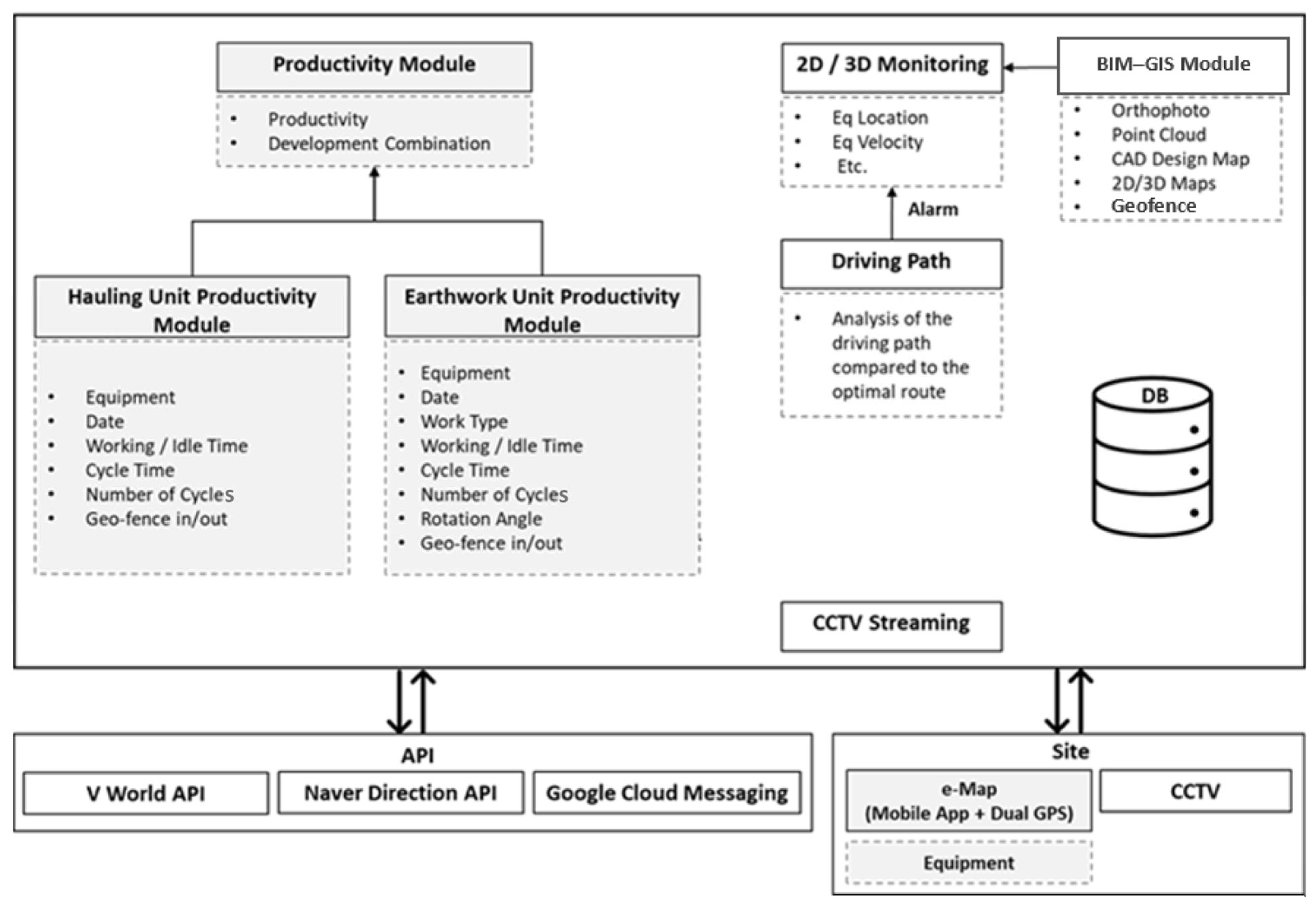
Figure 1. System Architecture of Intelligent Fleet Telematics System.
Applsci 16 01115 g001
Figure 2. System Data Processing Workflow Diagram.
Applsci 16 01115 g002
Figure 3. (a) e-Map Structure; (b) e-Map Interface Protocol.
Applsci 16 01115 g003
Figure 4. The e-Map Installation and Data Analysis Method.
Applsci 16 01115 g004
Figure 5. (a) Excavation Equipment Report Concept; (b) Grading Equipment Report Concept; (c) Hauling Equipment Report Concept.
Applsci 16 01115 g005
Figure 6. (a) Hauling Equipment Unit Productivity Flow Chart; (b) Excavation Equipment Motion Classification Algorithm.
Applsci 16 01115 g006
Figure 7. Excavation Equipment Motion Classification Algorithm.
Applsci 16 01115 g007
Figure 8. Grading Equipment Motion Classification Algorithm.
Applsci 16 01115 g008
Figure 9. Grading Equipment Unit Productivity Flow Chart.
Applsci 16 01115 g009
Figure 10. (a) System Evaluation and Feasibility Validation Process; (b) Measurement Environment; (c) Sample Measurement Document; (d) Sample Comparison Data Sheet.
Applsci 16 01115 g010
Figure 11. Unit productivity calculations of different construction machines: (a) Excavator Working/Idle Time Result; (b) Excavator Cycle Time Result; (c) Dump Truck Working/Idle Time Result; (d) Dump Truck Cycle Time Result; (e) Dozer Working/Idle Time Result; (f) Dozer Cycle Time Result.
Applsci 16 01115 g011
Figure 13. Construction machines working analysis under different conditions: (a) Productivity Analysis Between Equivalent Excavator; (b) Productivity Analysis Between Same Site Excavator; (c) Productivity Analysis by Number of Dump Trucks in the Same Site; (d) Soil Preparation Performance Rate Between Excavators.
Applsci 16 01115 g013
Table 1. Summary of the literature on fleet monitoring and productivity estimation for earthwork equipment.
Author(s)/
Year
Method/GoalResearch OutputResearch Gap
Addressed in this Research
Alshibani and Moselhi, 2016
[39]
GPS receivers on dump trucks calculate equipment operation cycles, while parameters, like earthwork volume, working hours, and costs, are input to measure earthwork productivity at the construction site.Dump truck operation cycle calculation.Consider other equipment working with dump trucks.
Lee et al., 2018 [40]Fleet management technology utilized to enhance fleet productivity and to introduce algorithms based on the ray casting algorithm for calculating dump trucks’ working time and idle time.Work motion classification as working and idle time of dump trucks using GPS data.(i) Work motion classification, Working/Idle for other construction equipment.
(ii) Equipment deployment combination.
Miller et al., 2021
[41]
A process for collecting data from multiple dump truck operations using a mobile app, control sensors, and web programs to identify inefficient operations through Cycle Time analysis was presented.Identify inefficient tasks using cycle time difference.Attaching sensors to dump trucks is not practical due to actual site conditions. Driver mobile is used to collect data.
Monnot and Williams, 2011 [42]The telematics data standards of the Association of Equipment Management Professionals (AEMP) are established for fleet monitoring.Established standard protocols for fleet management.Monitoring equipment productivity information is considered. Location and heading protocol is used for construction equipment.
Pegorer et al., 2013 [22]Discusses the issue that not all manufacturers are using standard protocols.
Dekate, 2013 [43]Evaluates the equipment’s actual lifespan and product reliability using PHM (Prognostics and Health Management) technology and the CAN bus protocol of construction equipment.
Kim et al., 2018 [44]A smartphone’s Inertial Measurement Unit (IMU) was used to gather rotation data from the excavator. The data were then classified into categories, such as Moving, Not Moving, Rotating Clockwise, and Rotating Anti-Clockwise, using the Random Forest algorithm. This classification enabled the analysis of the excavator’s Cycle Time.Analyze productivity using machine learning.Cycle analysis of earthwork equipment with an excavator is considered.
Kukreja et al., 2020 [45]The optimal route for dump truck operations was proposed using GPS, Google API, and GSM to minimize cycle time.Naver API utilization.(i) Dump truck productivity analysis.
(ii) Calculation of optimal deployment combination.
Table 2. Stop Motion Feasibility Verification Result.
ClassificationActual MotionRun Time
(s)
Average Moving Distance per Second (m)Average (m)Standard Deviation/CI 95% (Range)
Low RPMForward230.780.770.017/0.77 (0.75~0.79)
Backward320.78
Forward320.75
Backward340.78
Forward350.74
Backward360.77
High RPMForward330.910.920.017/0.92 (0.90~0.94)
Backward330.93
Forward310.94
Backward340.93
Forward350.90
Backward340.90
Applsci 16 01115 i001
Measurement Time: 00:06:43 (Including Stop).
Table 3. Rotating Motion Feasibility Verification Result.
ClassificationActual
Motion
Run Time
(s)
Average Angle Variance
per Second (°)
Average (°)Standard Deviation/CI 95% (Range)
Loading
Work
Type
Rotating419.7123.713.96/23.72 (20.40~27.03)
Rotating324.14
Rotating323.33
Rotating329.22
Rotating421.85
Rotating329.63
Rotating418.79
Rotating323.06
Slope
Work
Type
Rotating214.7719.215.17/19.21 (14.88~23.54)
Rotating125.41
Rotating113.61
Rotating222.81
Rotating219.13
Rotating114.21
Rotating417.07
Rotating626.67
Applsci 16 01115 i002
Measurement Time: 00:07:54 (Including Stop and Digging/Loading).
Table 4. Soil Preparation Motion Feasibility Verification Result.
ClassificationActual MotionRun Time
(s)
Average Angle Variance
per Second (°)
Average (°)Standard Deviation/CI 95% (Range)
Loading
Work
Type
Soil Preparation223.215.662.65/5.66 (3.44~7.88)
Soil Preparation134.01
Soil Preparation221.97
Soil Preparation149.74
Soil Preparation164.60
Soil Preparation206.38
Soil Preparation128.18
Soil Preparation67.17
Applsci 16 01115 i003
Measurement Time: 00:20:00 (Including Stop and Digging/Loading).
Table 5. Digging and Loading Motion Feasibility Verification Result.
ClassificationActual MotionRun Time
(s)
Average (s)Standard Deviation/CI 95% (Range)
Loading
Work
Type
Digging106.53.6/6.4 (4.21~8.79)
Loading3
Digging6
Loading4
Digging7
Loading5
Digging7
Loading4
Digging10
Loading4
Digging15
Loading3
Applsci 16 01115 i004
Measurement Time: 00:08:31 (Including Stop).
Table 6. Forward and Reverse Motion Feasibility Verification Result.
ClassificationActual MotionRun Time
(s)
Average Angle Margin (°)Average (°)Standard Deviation/CI 95% (Range)
Spreading
Work
Type
Forward7172.15180.593.91/180.59 (177.32~183.86)
Forward10181.01
Forward4186.14
Forward18182.49
Forward69180.69
Forward100180.65
Forward40181.65
Forward39179.94
Backward810.305.023.30/5.02 (2.26~7.78)
Backward152.80
Backward89.65
Backward91.68
Backward775.35
Backward761.97
Backward494.48
Backward553.92
Applsci 16 01115 i005
Measurement Time: 00:35:06 (Including Stop).
Table 7. Excavation Motion Algorithm Parameter Accuracy Result.
Actual Measurement
EquipmentMotionNote
Digging/LoadingSoil PreparationRotatingMovingStop
Excavation6357479345979530
Monitoring (Determining Parameter)
EquipmentMotionNote
Digging/LoadingSoil PreparationRotatingMovingStop12°, 0.5 m,
1°, 20 s
Excavation6593220347480537
Error (%)3.7%−54.1%0.4%1.3%1.3%
Monitoring (Case 1: Rotating Parameter Test)
EquipmentMotionNote
Digging/LoadingSoil PreparationRotatingMovingStop15°, 0.5 m,
1°, 20 s
Excavation66272393021469548
Error (%)4.2%−50.1%−12.7%493.7%3.4%
EquipmentMotionNote
Digging/LoadingSoil PreparationRotatingMovingStop10°, 0.5 m,
1°, 20 s
Excavation6450153376472465
Error (%)1.5%−68.1%8.8%−8.9%−12.3%
Monitoring (Case 2: Moving Parameter Test)
EquipmentMotionNote
Digging/LoadingSoil PreparationRotatingMovingStop12°, 1.0 m,
1°, 20 s
Excavation6618239347422551
Error (%)4.1%−50.1%0.4%−72.2%4.0%
EquipmentMotionNote
Digging/LoadingSoil PreparationRotatingMovingStop12°, 0.1 m,
1°, 20 s
Excavation47673834742301324
Error (%)−25.0%−92.1%0.4%2812.7%−38.9%
Monitoring (Case 3: Soil Preparation Parameter Test)
EquipmentMotionNote
Digging/LoadingSoil PreparationRotatingMovingStop12°, 0.5 m,
3°, 20 s
Excavation6593110347480647
Error (%)3.7%−77.0%0.4%1.3%22.1%
EquipmentMotionNote
Digging/LoadingSoil PreparationRotatingMovingStop12°, 0.5 m,
0.5°, 20 s
Excavation6593289347480468
Error (%)3.7%−39.7%0.4%1.3%−11.7%
Monitoring (Case 4: Stop Parameter Test)
EquipmentMotionNote
Digging/LoadingSoil PreparationRotatingMovingStop12°, 0.5 m,
1°, 30 s
Excavation6983103347480264
Error (%)9.8%−78.5%0.4%1.3%−50.2%
EquipmentMotionNote
Digging/LoadingSoil PreparationRotatingMovingStop12°, 0.5 m,
1°, 10 s
Excavation16234273474803761
Error (%)−97.5%615.4%0.4%1.3%609.6%
Measurement Time: 3:01:44.
Table 8. Grading Motion Algorithm Parameter Accuracy Result.
Actual Measurement
EquipmentMotionNote
ForwardBackwardStop
Grading5815941136
Monitoring (Determining Parameter)
EquipmentMotionNote
ForwardBackwardStop90°, 0.1 m
Grading5925941125
Error (%)1.9%0.0%−1.0%
Monitoring (Case 1: Forward, Backward Parameter Test)
EquipmentMotionNote
ForwardBackwardStop180°, 0.1 m
Grading3737741164
Error (%)−35.8%30.3%2.5%
EquipmentMotionNote
ForwardBackwardStop10°, 0.1 m
Grading6405071164
Error (%)10.2%−14.6%2.5%
Monitoring (Case 2: Stop Parameter Test)
EquipmentMotionNote
ForwardBackwardStop90°, 1.0 m
Grading5375471227
Error (%)−7.6%−7.9%8.0%
EquipmentMotionNote
ForwardBackwardStop90°, 0.5 m
Grading5685791164
Error (%)−2.2%−2.5%2.5%
Measurement Time: 00:38:31.
Table 9. Hauling Equipment Algorithm Feasibility Verification Result.
Actual Measurement
EquipmentLoading Zone InLoading Zone OutTime RequiredNumber of Cycles (sum)
DT 801410:16:1310:23:450:07:327
10:27:2810:35:380:08:10
10:39:2010:48:520:09:32
10:53:5511:02:190:08:24
11:08:0311:16:130:08:10
11:21:4511:30:100:08:25
11:35:4711:43:450:07:58
AVG10:54:3911:02:570:08:19
Monitoring
EquipmentLoading Zone InLoading Zone OutTime RequiredNumber of Cycles (sum)
DT 801410:16:0010:23:370:07:377
10:27:2410:35:270:08:03
10:39:1410:48:330:09:19
10:53:4511:02:160:08:31
11:08:0011:16:070:08:07
11:21:4111:30:030:08:22
11:35:4011:43:310:07:51
AVG10:54:3211:02:480:08:16
Error (sec)0:00:070:00:100:00:03
Measurement Time: 1:27:32.
Table 10. Excavation and Grading Equipment Algorithm Feasibility Verification Result.
Measurement Time: 00:43:07
Actual Measurement
EquipmentCycle Time (avg, s)Cycle Time (sum, s)Number of Cycles (sum)Idle Time
Excavation equipment201573790:05:27
Monitoring
EquipmentCycle Time (avg, s)Cycle Time (sum, s)Number of Cycles (sum)Idle Time
Excavation equipment19.691595810:05:35
Error (%)−1.5%1.4%2.5%2.4%
Absolute error (Δ)−0.31 s+22 s+2+0:00:08 (+8 s)
Measurement Time: 3:01:44
Actual Measurement
EquipmentCycle Time (avg, s)Cycle Time (sum, s)Number of Cycles (sum)Idle Time
Excavation equipment2175873600:08:50
Monitoring
EquipmentCycle Time (avg, s)Cycle Time (sum, s)Number of Cycles (sum)Idle Time
Excavation equipment21.3277423630:08:57
Error (%)1.5%2.0%0.8%1.3%
Absolute error (Δ)+0.32 s+155 s+3+0:00:07 (+7 s)
Measurement Time: 00:38:31
Actual Measurement
EquipmentCycle Time (avg, s)Cycle Time (sum, s)Number of Cycles (sum)Idle Time
Grading equipment621065170:18:56
Monitoring
EquipmentCycle Time (avg, s)Cycle Time (sum, s)Number of Cycles (sum)Idle Time
Grading equipment62.821068170:18:45
Error (%)1.3%0.3%0.0%−1.0%
Absolute error (Δ)+0.82 s+3 s0−0:00:11 (−11 s)
Table 11. Dump Truck Deployment According to Excavator Operating Efficiency.
Yeongjong–Cheongna
Ex Komatsu
(Spec: 2.0 m3)
Ex Doosan
(Spec: 1.5 m3, MG)
JuneAugustSeptemberOctober
① Dump Truck Shift Time (s)29292929
② Number of Excavator Cycles per Dump Truck7799
Excavator Cycle Time (avg, s)26.025.219.519.5
③ Excavator Loading Time (s)182176175175
Number of Dump Truck Cycles (avg)123129132127
Number of Dump Truck Deployments3444
Excavator Working Time + Idle Time (avg, h)9998.8
④ Number of Dump Truck Cycles at Excavator’s Maximum Working Capacity154158159155
⑤ Number of One Dump Truck Cycles (avg)41353433
⑥ Calculated Dump Truck Recommendation for Excavator Combination3.84.54.74.7
Actual Number of Dump Trucks Deployed3444
Table 12. Case Study Comprehensive Indicators.
MarchAprilJuneAugustSeptemberOctober
Working Time
(avg, h)
Excavator7.67.58.18.28.48.0
Dump Truck--8.48.38.08.1
Dozer--8.8---
Idle Time
(avg, h)
Excavator0.91.10.90.80.60.8
Dump Truck--0.60.71.00.7
Dozer--0.2---
Cycle Time
(avg, s)
Excavator21.321.826.025.219.519.5
Dump Truck--12.113.214.214.4
Dozer--1.8---
Number of Cycles
(sum)
Excavator1037641574677852013,78923,834
Dump Truck--737128717122654
Dozer--6093---
Angle (avg, °)Excavator97.093.198.784.281.988.2
Volume (m3)Excavator--935417,04120,68335,750
Dump Truck--10,70118,68724,85838,536
Ex-Bucket--1.781.811.381.43
DT-Load--12.4412.7012.4612.87
Drone--916916,33921,33534,166
Productivity
(m3/h)
Excavator114.6113.6153.9171.7163.2180.4
Dump Truck--47.2649.0746.4847.32
Deployment Dump CycleDump Truck--154158159155
Deployment DumpDump Truck--3.84.54.74.7
Disclaimer/Publisher’s Note: The statements, opinions and data contained in all publications are solely those of the individual author(s) and contributor(s) and not of MDPI and/or the editor(s). MDPI and/or the editor(s) disclaim responsibility for any injury to people or property resulting from any ideas, methods, instructions or products referred to in the content.