Collaborative Coverage Path Planning for AUV Formations: Dual-Layer PSO-Voronoi Partitioning for Time-Based Load Balancing Combined with BINN

Abstract

In multi-AUV collaborative underwater coverage operations, the fundamental principle of load balancing is temporally rather than spatially defined. Traditional partition schemes that equalize area or grid counts suffer from a critical fallacy: they assume a linear mapping from geometry to working time, which collapses in the presence of irregular obstacles. This paper demonstrates that temporal load imbalance causes some AUVs to finish prematurely and remain idle—consuming power and fighting currents while their counterparts struggle with topologically complex sub-regions. To address this, we propose a dual-layer nested Particle Swarm Optimization (PSO) framework for Voronoi partitioning, where the outer layer coarsely initializes grid counts, while the inner layer directly minimizes the makespan and time variance derived from actual BINN-simulated coverage paths. This two-stage PSO architecture effectively resolves the nonlinear mismatch between geometric partitioning and real operation time, redefining load balancing from a geometrical abstraction to a temporally grounded, operationally relevant metric. Furthermore, we rigorously distinguish the intrinsic nature of coverage path planning (CPP) from Traveling Salesman Problem (TSP)-based point routing—the latter generates discontinuous, sharp-turning trajectories that violate the kinematic constraints of side-scan sonar payloads and cause critical data gaps. The proposed architecture yields a standard deviation of mission times that is an order of magnitude lower than area-based heuristics, while maintaining kinematically feasible continuous sweeps. Crucially, we explicitly delineate the operational boundary of this framework: it is purpose-built for static, pre-surveyed environments where offline computational overhead (approximately 8 min) is a justifiable investment against a 3 h optimal field execution.

1. Introduction

1.1. Background

Traditionally, tasks such as area search and underwater terrain exploration have often relied on a single autonomous underwater vehicle. However, as the scale of the operational area continues to expand, single-AUV solutions increasingly suffer from low operational efficiency, concentrated reliability risks, and limited adaptability. Multi-AUV cooperation has therefore become an essential approach to overcoming the performance limitations of individual platforms. Nevertheless, underwater environments impose severe constraints on cooperative operation. Acoustic communication is characterized by low bandwidth, long latency, poor reliability, and strong susceptibility to environmental disturbances. In addition, underwater vehicles generally lack access to global navigation satellite signals. As a result, AUV formations cannot rely on frequent and high-volume information exchange in the same way as autonomous aircraft. Designing efficient and conflict-free task planning methods for multi-AUV systems under such communication-constrained conditions has thus become a central challenge. This problem is of both practical engineering significance and theoretical research value. However, a critical oversight persists in current literature: load balancing is almost universally defined in the spatial domain—equal area, equal grid count, or equal cell distribution. This implicit assumption presumes a linear mapping from area to working time. In reality, the presence of concave obstacles and narrow passages causes a nonlinear inflation of traversal time for a given geometry. More importantly, for underwater operations, the consequence of temporal imbalance is far more severe than mere inefficiency. An AUV that completes its sub-region early has no productive role except to remain idle at the rendezvous point. During this idle period, the vehicle continues to drain its batteries against unsteady ocean currents and must actively maintain its position without collecting scientific data—a pure waste of onboard energy and an increased risk of navigation drift. Consequently, in the static, pre-surveyed underwater coverage scenarios focused on in this paper, temporal balancing is not merely an optimization goal; it is a practical necessity to maximize the effective utilization of every vehicle’s finite underwater endurance.

1.2. Related Work

Research on multi-AUV coordination has historically coalesced around three interconnected themes: region partitioning, coverage path planning (CPP), and collaborative system architecture [1].

The objective of region partitioning is to carve the overall operational area into sub-regions that allocate workload fairly among vehicles [2]. Existing solutions broadly fall into geometric, clustering-based, and metaheuristic categories. Geometry-driven approaches, such as Voronoi diagrams [3], are computationally lean but struggle to accommodate irregular obstacle fields [1]. Clustering methods—including K-means++ [4] and fuzzy C-means [5]—rely on Euclidean proximity and thus break down in non-convex or narrow-lane environments [6]. Alternative geometric partitioning tools, such as Delaunay triangulation [7], and density-based clustering methods (e.g., DBSCAN [8] and HDBSCAN [9]) have also been explored for multi-robot area coverage. Nevertheless, the standard Delaunay triangulation requires a constrained variant to accommodate concave obstacles, whereas density-based clustering approaches are generally sensitive to parameter selection. Moreover, density-based clustering approaches are gaining traction in underwater platforms, yet their systematic application at the region-partitioning level—especially their deep coupling with coverage path planning (CPP)—remains conspicuously underexplored. More recently, multi-agent reinforcement learning [10] and graph neural networks [11] have been proposed, yet they incur heavy training overhead and generalize poorly across unseen terrains, all while presupposing reliable communication links.

A critical observation is that area or grid count has long served as a convenient proxy for workload, but this geometric abstraction is not equivalent to actual working time. The presence of concave obstacles and narrow passages causes a nonlinear inflation of traversal time for a given geometry. Recognizing this, several recent studies have begun to address temporal load balancing in multi-robot CPP. For instance, game-theoretic decomposition methods directly use Dubins path costs for task reallocation, explicitly breaking the conventional assumption that “balanced area guarantees balanced coverage time” [12]. Auction-based approaches, such as SCoPP, aim at time-efficient coverage with workload-balanced plans by coupling partitioning with boundary bidding [13]. Graph-based direct partitioning methods also adopt balanced workload as a core criterion [14], and iterative task decomposition and allocation frameworks have been shown to reduce inter-UAV execution time gaps substantially [15]. These works confirm that temporal balancing is not an unexplored direction. However, they typically adopt a loosely coupled paradigm: partitioning is first determined, and path time is then evaluated or locally adjusted. The path cost used for balancing is often an analytical approximation (e.g., Dubins distance) or a heuristic estimate, rather than being derived from the actual coverage path that will be executed. Consequently, the partitioning decision and the true traversal time remain disconnected, and the optimization does not benefit from closed-loop feedback from path simulation to region shaping. This is the methodological gap that the present work aims to address.

A CPP algorithm must produce a path that exhaustively sweeps a given region while minimizing redundancy, energy draw, and steering effort [16]. The core difficulty lies in tailoring the sweep pattern to the specific geometry of each sub-region [17]. Among classical methods, the Spanning Tree Coverage (STC) algorithm guarantees completeness but tends to generate jagged, turn-heavy trajectories that impose unnecessary mechanical stress [18]. Others adjust track spacing dynamically to reduce overlap [19] or reformulate CPP as a Traveling Salesman Problem over sub-regions [20]. It is tempting to formulate coverage as a TSP over grid centroids, but this commits a category error: TSP optimizes discrete point-to-point hops, whereas CPP is inherently a continuous area-sweeping problem. For an underactuated AUV with side-scan sonar, a TSP-derived path is physically untenable: sharp turns break sensor swath continuity, causing unrecoverable data gaps, while frequent reorientations accelerate mechanical fatigue on thrusters. Thus, TSP solves the wrong problem class; underwater CPP must optimize continuous, directionally persistent sweeps (e.g., lawnmower patterns), not point-to-point distances. Evolutionary search techniques, including genetic algorithms [21] and differential evolution with Q-learning-based strategy selection [22], have also demonstrated promising performance in path planning, yet their integration with temporally aware load balancing remains underexplored in specific scenarios such as multi-AUV underwater coverage. On the optimization front, exact cellular decomposition combined with differential evolution [23] can shorten execution times but still provides no guarantee of global optimality given the absence of energy-aware heuristics. Internal-spiral algorithms achieve full coverage, yet their applicability shrinks with fleet size [24]. The Glasius bio-inspired neural network (GBNN) offers an elegant dynamic-field solution for coverage, though it takes little account of starting-position sensitivity [25]. For multi-AUV systems, the tight coupling between partitioning and intrazone routing—and the need to resolve both in service of time-balancing—remains conspicuously underexplored.

Centralized frameworks provide a global view and superior optimality potential, but they introduce single points of failure and scalability bottlenecks. Distributed architectures, by contrast, are robust and scalable but struggle to reach globally consistent decisions. Hybrid schemes—and particularly the “plan centrally, execute distributively” paradigm—offer an attractive middle ground, preserving global coordination while granting local reactivity [26]. This is the architectural philosophy we adopt here.

1.3. Research Motivation and Contributions

Building on the above observations, we introduce an architecture that couples dual-layer PSO-driven Voronoi partitioning with BINN-based coverage routing, under a centralized planning/distributed execution model. The methodological novelty of this work lies not in the individual techniques—Voronoi partitioning, PSO, and BINN are well established—but in the nested coupling mechanism that renders the partitioning process responsive to the nonlinear, topology-dependent time costs of coverage sweeps. Our specific contributions are threefold:

A path-cost-driven nested PSO formulation with closed-loop feedback. Unlike existing time-balancing approaches that evaluate path time after partitioning, our second-layer PSO directly minimizes the makespan and time dispersion derived from actual BINN-simulated coverage paths. This embeds a path-simulation-based time cost into the inner optimization loop, allowing the Voronoi seeds to be reshaped by the true traversal costs. This redefines load balancing from a geometric proxy to a temporally grounded, operationally relevant metric, and establishes a closed-loop coupling between region partitioning and intrazone routing.

A hybrid CPP engine that ensures the physical validity of the time feedback. BINN generates smooth, forward-looking primary sweeps, while A* intervenes locally to escape deadlocks and close paths back to the home position. This integration is not merely a combination of existing tools; it guarantees that the time signal used in the outer layer reflects kinematically feasible, continuous coverage paths. Without such a path generator, temporal optimization would operate on a cost model disconnected from actual sweep execution—a prerequisite that is often overlooked in loosely coupled time-balancing methods.

A systematic benchmarking campaign that isolates the contributions of partitioning and path generation. We compare against four representative alternative architectures using multiple performance dimensions, explicitly separating the effects of partitioning strategy and path generation strategy. This delineates the strengths and appropriate deployment contexts of the proposed framework and provides empirical evidence that the closed-loop coupling—rather than any single component—is responsible for the order-of-magnitude reduction in time dispersion.

2. Problem Formulation

This paper considers the problem of region partitioning and coverage mission planning for a formation of AUVs operating within a static two-dimensional maritime area. Each operational AUV undertakes a full three-stage mission profile: departing from a shared central rendezvous point, transiting to its assigned sub-region, performing exhaustive sweep coverage throughout the sub-region, and ultimately returning to the central point upon survey completion. The overarching objectives are to achieve full coverage of all traversable areas, balance mission durations across the AUV fleet, minimize the global maximum mission completion time (makespan), and reduce redundant coverage.

Conventional spatial partitioning schemes, which equalize sub-region area or grid count, inherently overlook disparities in transit distance between proximal and distal sub-regions, as well as the nonlinear traversal time introduced by complex obstacle topologies. This creates a fundamental mismatch between geometric workload balance and actual temporal load equilibrium, which constitutes the core problem addressed in this work.

We model the operational area as a rectangle, discretized into a two-dimensional grid map. The team consists of one mother AUV and five homogeneous operational AUVs. The mother AUV is responsible for transporting the five operational AUVs from the shore base to the geometric center of the designated mission area, then performing centralized offline decision-making and task assignment, after which it deploys the operational AUVs to execute the coverage survey. All five operational AUVs start from the mother AUV; upon completing their sweeps, they return to the mother AUV for recovery and offload the collected data. Let $S={\{(x_i,y_i)\}}_{i=1}^N,N=5$ denote the Voronoi seed set that defines the partition, and let $P_i=\{p_{i,1},p_{i,2},\cdots ,p_{i,M_i}\}$, where $p_{i,j}=(x_{i,j},y_{i,j})$, denote the grid-coordinate waypoint sequence of $AU{V}_i$. Thus, the planning problem can be stated as a constrained multi-objective optimization over $(S,\{P_i\})$: the primary objective is to minimize the maximum mission duration, and the secondary objective is to minimize the dispersion of the mission durations across AUVs. The constraints are fourfold: (i) coverage completeness—every passable grid cell must be covered by at least one AUV’s sonar swath; (ii) a non-overlapping Voronoi partition—the sub-regions must be mutually exclusive, and their union must equal the set of all passable cells; (iii) obstacle avoidance—no path segment may enter an obstacle cell; and (iv) kinematic feasibility—consecutive waypoints must differ by at most one grid cell, and turning is subject to directional inertia. The AUVs are modeled as discrete-grid point masses with position $(x,y)$, constant cruise speed $v=3 \mathrm{m}/\mathrm{s}$, grid resolution $\Delta =200 \mathrm{m}$, and eight-neighborhood motion, so that directional inertia yields smooth, lawnmower-like trajectories.

To keep the problem tractable, we adopt the following assumptions:

• Communication and control strategy: A “centralized planning—distributed execution” strategy is adopted. The mother AUV performs offline global planning (region partitioning and initial path generation) using prior environmental information. During execution, each operational AUV follows its assigned path, requiring only minimal real-time inter-AUV communication to avoid communication conflicts, which is suitable for the bandwidth-limited nature of underwater acoustic communication.
• Environmental obstacles and inter-AUV collision avoidance: Static obstacles in the mission area (e.g., reefs and shipwrecks) are known a priori and represented as impassable grid cells. Under the premise that the assigned sub-regions are mutually non-overlapping, AUVs face only a slight collision risk during the departure and return phases, which can be resolved through simple time-slot scheduling and does not affect the core partitioning results.
• AUV deployment and energy: All AUVs are homogeneous, with identical cruising speed (3 m/s) and sensor detection width (equal to one grid cell side length of 200 m). Each AUV has sufficient on-board energy to complete its assigned full-coverage task and return; thus, energy acts as a constraint for time balancing but does not appear as a limiting factor on feasibility in simulations. This paper does not undertake bottom-level energy modeling; its core objective is to employ mission-level temporal balancing to eliminate the idle-time energy waste of early finishers and to prevent late finishers from having insufficient energy to complete the mission.
• Mission completeness and coverage verification: Coverage is considered complete when every passable grid cell has been visited by at least one AUV’s sensor. The path planning algorithm must guarantee 100% coverage within each assigned sub-region. The grid cell size is set equal to the sensor detection width, ensuring that a single pass along grid lines fully covers each cell and thereby simplifying coverage verification. At the region boundary, half of the swath extends beyond the mission area, which guarantees complete coverage of boundary cells. Moreover, the actual sonar swath width is larger than 200 m; it is limited to 200 m to account for coverage gap effects and other potential factors.

This study considers static environments with known obstacle distributions; dynamic scenarios are deferred to future work (a detailed discussion of applicability boundaries is provided in Section 3.2.3). Based on the above assumptions, the core challenges are as follows: (1) how to partition the region to minimize the maximum mission duration across AUVs; and (2) for a given sub-region, how to generate a low-redundancy, smooth coverage path.

This work focuses on pre-planned offshore survey tasks with a priori known static obstacle information, rather than real-time online re-planning for unknown dynamic environments.

3. Methodology

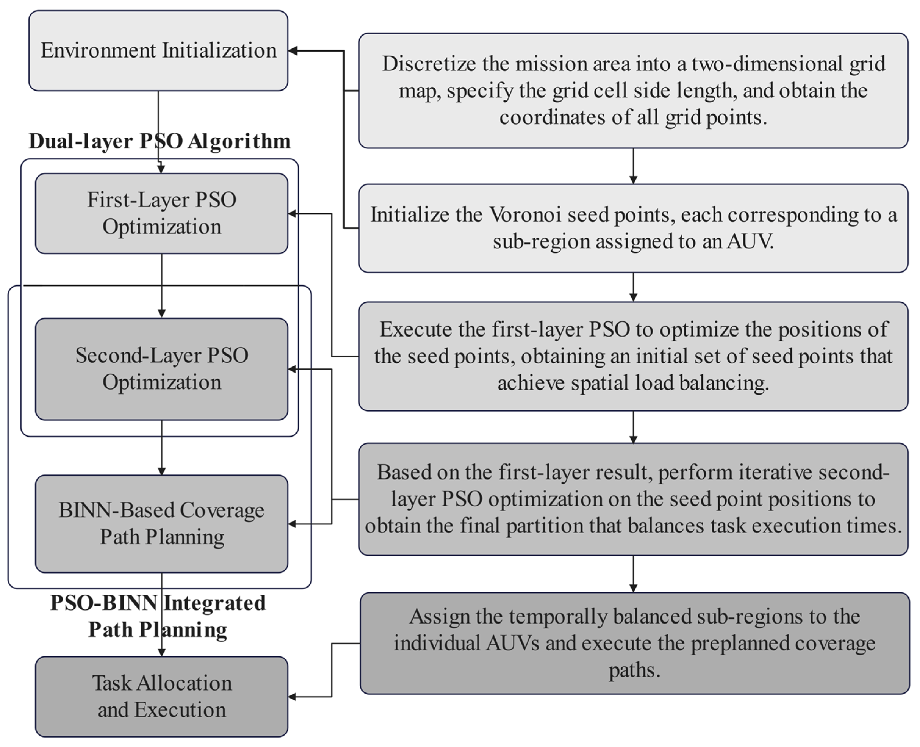
To address the above problems, this paper designs a hierarchical, modular algorithmic architecture. The architecture first addresses the macroscopic region allocation problem, then handles the microscopic individual path planning problem. The overall workflow is illustrated in Figure 1.

3.1. Voronoi Diagram-Based Region Partitioning

The Voronoi diagram, which is also referred to as the Thiessen polygon, is a region partitioning structure widely used in computational geometry [27]. Given a set of $N$ seed points $P=\{p_1,p_2,\cdots p_N\}$ in the plane, each free grid cell is assigned to the nearest seed point $p_i$, which yields a partition of the plane. The task allocation problem therefore reduces to locating an optimal set of seed points $P$.

3.2. Optimal Voronoi Partitioning via Dual-Layer PSO

The pivotal innovation of this research lies in employing a dual-layer nested Particle Swarm Optimization (PSO) framework to search for optimal seed point locations. The standard PSO algorithm keeps a population consisting of “particles”, each representing a candidate solution [28]. Each particle has a position $x$ and velocity $v$, updated according to Equations (1) and (2) based on its own historical best position and the global historical best position of the population.

$$v_{\left(t+1\right)}=w·v_{\left(t\right)}+c_1·r_1·\left(p_{best}-x_{\left(t\right)}\right)+c_2·r_2·\left(g_{best}-x_{\left(t\right)}\right)$$

(1)

$$x_{(t+1)}=x_{(t)}+v_{(t+1)}$$

(2)

where $w$ is the inertia weight, $c_1$ and $c_2$ are the cognitive and social learning factors, respectively, and $r_1$ and $r_2$ are uniformly distributed random numbers in $[0,1]$.

3.2.1. First-Layer PSO: Grid Count Balancing Optimization

The objective of the first layer is to rapidly achieve coarse task-load balancing using grid count as a surrogate metric. For $N=5$ AUVs, a particle represents a set of five 2D seed points, forming a 10-dimensional vector $x=[x_1,y_1,x_2,y_2,\cdots ,x_5,y_5]$. The objective function $f_1$ minimizes the difference between the maximum and minimum grid counts across regions, as shown in Equation (3).

$$f_1(S)=\underset{k}{\max } N_k-\underset{k}{\min } N_k$$

(3)

where $N_k$ is the number of free grid points in region $k$.

For the first-layer PSO, the swarm size is set to 50 particles, and the maximum number of iterations is 100. Since the first layer only performs coarse partitioning of regional grid counts, PSO can achieve rapid convergence. For the initialization strategy, this paper adopts a stripe-based intelligent initialization scheme rather than purely uniform random sampling: the operational area is equally divided along the x-axis into five vertical stripes; the x-coordinates of the five seed points are uniformly sampled within their corresponding stripes, while the y-coordinates are uniformly sampled over the entire y-range of the operational area. This strategy ensures a spatially uniform distribution of the initial population and prevents premature convergence caused by seed-point clustering. If the difference between the maximum and minimum regional grid counts exhibits no improvement for 20 consecutive iterations before the 100th iteration, early stopping is triggered. In addition, to avoid local optima, a population-diversity maintenance mechanism is introduced: when the global best value has not been updated for 10 consecutive iterations, the worst 20% of particles in terms of fitness are reinitialized using the above stripe-based sampling strategy, thereby restoring population diversity. The core parameter settings are as follows:

Initial inertia weight, ${\omega }_0=0.9$. This value preserves particle momentum and thereby promotes broad global exploration during the early iterations.

Inertia decay factor, set to 0.98. The inertia weight decays exponentially with each iteration, progressively shifting the swarm from exploration to local exploitation.

Cognitive coefficient, $c_1=2.0$. This parameter weights the attraction of each particle toward its own historical best position, following standard PSO practice.

Social coefficient, $c_2=2.0$. This parameter weights the attraction of each particle toward the global best position of the entire swarm, also following standard PSO practice.

3.2.2. Second-Layer PSO: Task Time Balancing Optimization

The second-layer PSO performs local fine-tuning around the balanced seed points $S^{(1)}$ obtained from the first layer, directly optimizing the temporal balance of task completion times.

The task time $T_k$ for $AU{V}_k$ is the sum of transit time, coverage time, and return time. The coverage path is generated by the BINN algorithm (Section 3.3), with a step count of $N_k^{\mathrm{cov}}$; the transit path and return path are planned by the A* algorithm (Section 3.4), with step counts of $N_k^{trans}$ and $N_k^{ret}$. The total step count is $M_k=N_k^{\mathrm{cov}}+N_k^{trans}+N_k^{ret}$, and the task time is $T_k={\displaystyle \frac{M_k\cdot \Delta }{v}}$, where $\Delta =200 \mathrm{m}$ is the grid cell side length and $v=3 \mathrm{m}/\mathrm{s}$ is the AUV speed.

To ensure the fitness function maintains a consistent physical meaning across all PSO generations, we use fixed theoretical bounds for normalization instead of population-wise extreme values. The objective function $f_2$ of the second-layer PSO is formulated as shown in Equations (4) and (5).

$$f_2(S)={\displaystyle \frac{\underset{k}{\max } T_k-T_{lower}}{T_{upper}-T_{lower}}}+\alpha \cdot {\displaystyle \frac{Std(T_1,\cdots T_K)-S_{lower}}{S_{upper}-S_{lower}}}$$

(4)

$$S_{upper}=T_{upper}-T_{lower}, S_{lower}=0$$

(5)

where $T_{upper}$ is the theoretical maximum time for a single AUV to cover all free grids (ideal straight-line without turns), $T_{lower}$ is the theoretical minimum makespan with perfectly equal workload, i.e., $T_{upper}/N$; $S_{upper}$ is the theoretical maximum standard deviation, and $S_{lower}$ is the theoretical minimum standard deviation. This fixed-bound normalization eliminates the adaptive scaling drift caused by population-based normalization, ensuring that the optimization direction remains stable throughout the evolution process. The weight coefficient $\alpha$ governs the relative priority between makespan minimization and time-dispersion minimization. Since reducing the maximum mission duration generally also compresses the idle waiting of early-finishing AUVs and thus tends to reduce the standard deviation of mission times, the makespan term should remain dominant, while the standard-deviation term serves as a secondary refinement. Accordingly, $\alpha$ should be kept relatively small. In preliminary simulations over multiple runs, $\alpha =0.1$ provided satisfactory and stable optimization results, and this value is therefore adopted. This normalization further ensures that both criteria are commensurate, preventing either term from dominating merely due to numerical scale.

Because each fitness evaluation in the second layer requires executing a complete BINN-based coverage path simulation for all AUVs, the computational cost is substantial. A smaller population is therefore adopted for local fine-tuning: the population size is set to 15 particles, and the maximum number of iterations is set to 30. This layer employs a localized initialization scheme: all particles are generated by superimposing zero-mean Gaussian noise on the optimal seed points output by the first-layer PSO. The noise standard deviation is set to 5% of the side length of the operational area, so that the second-layer search concentrates on the neighborhood of the high-quality solution identified by the first layer, thereby substantially improving convergence efficiency. The algorithm terminates upon reaching the maximum of 30 iterations, with no additional early-stopping mechanism. The core parameter settings are as follows:

Initial inertia weight, ${\omega }_0=0.7$. A lower initial inertia is adopted to prioritize local exploitation, since the first layer already provides a high-quality starting point.

Inertia decay factor, set to 0.98. This gradually narrows the search granularity as iterations proceed.

Cognitive coefficient, $c_1=2.0$. This retains the standard weight for personal best attraction.

Social coefficient, $c_2=1.5$. The reduced social weight prevents over-convergence and preserves moderate swarm diversity during fine-tuning.

3.2.3. Scope of Applicability, Modeling Abstraction, and Validation Boundaries

Before proceeding to the experimental validation, it is imperative to delineate the operational envelope of the proposed nested optimization framework. The reliance on repeated BINN simulations within the inner PSO loop incurs non-negligible computational overhead, which scales with grid resolution and fleet size. Consequently, this algorithm is specifically designed and recommended for the following deployment scenarios:

• Static and fully surveyed environments, where the obstacle map (e.g., reefs, pipelines, and wreckages) is known a priori from bathymetric surveys.
• Strategic offline planning, where a one-time computational investment of approximately 8 min is amortized over a 2–3 h long field mission (i.e., planning time accounts for about 5% of the total operational timeline).
• Time-critical formation missions, where synchronizing the completion times of all AUVs significantly reduces idle energy waste and minimizes the risk associated with prolonged underwater station-keeping.

Conversely, this framework is explicitly not recommended for highly dynamic environments (e.g., areas with moving obstacles or sudden and unpredictable current shifts) or for scenarios demanding rapid online re-planning (within sub-5 min response windows). In such cases, the geometric heuristics (e.g., sector partitioning) or reactive methods, despite their suboptimal makespan, would be more appropriate due to their negligible computational latency.

Before proceeding to experimental validation, it is necessary to further clarify the modeling abstraction level and the corresponding validation scope of the proposed framework. This study is positioned at the mission planning layer, focusing on region partitioning and waypoint-level coverage path scheduling, rather than explicit modeling of low-level AUV dynamics and control constraints. Specifically, six-degree-of-freedom hydrodynamics, minimum turning radius, curvature continuity, and trajectory tracking errors are outside the scope of this work. This abstraction allows the paper to concentrate on the algorithmic-level interplay between partition strategies and path topology in shaping mission-time balance, while leaving a clear interface for subsequent engineering extensions that incorporate dynamic constraints. Importantly, this modeling simplification does not undermine the validity of the proposed framework at the planning layer: in static, pre-surveyed environments, the smooth primary sweeps generated by BINN already exhibit strong directional persistence and low turning frequencies, enabling reliable assessment of mission-time balancing at the planning level. Consequently, the operational boundary of this framework should be understood as follows: offline strategic planning in static environments, validated at the mission planning layer, where performance metrics reflect topological-level coordination efficiency rather than execution accuracy after full dynamic simulation.

3.2.4. Computational Complexity Analysis

Let $G=N_g^2$ be the number of grid cells, $N$ the number of AUVs and Voronoi seeds, and $P_1,I_1$ and $P_2,I_2$ the swarm sizes and iteration limits of the two PSO layers. The first layer evaluates a particle by constructing a Voronoi partition and counting free cells, which costs $O(NG)$. Its total cost is $O(P_1{I}_{1}NG)$, which is low and serves only as coarse initialization.

The second layer dominates the runtime. Each fitness evaluation requires a complete BINN coverage simulation for every AUV, together with A* calls for deadlock escape and return-path closure. For $AU{V}_k$, let $G_k$ and $L_k$ denote the number of cells in its sub-region and the number of BINN path steps. One particle evaluation costs $O({\displaystyle \sum _{k=1}^N{G}_k{L}_k})$, so the second-layer cost is $O(P_2{I}_2{\displaystyle \sum _{k=1}^N{G}_k{L}_k})$. Since $L_k=O(G_k)$, this is approximately $O(P_2{I}_2{\displaystyle \sum _{k=1}^N{G}_k^2})$. With $P_2=15$, $I_2=30$, $N=5$, and $G=625$, the second layer performs up to 450 particle evaluations, i.e., 2250 BINN simulations, which accounts for the measured runtime of about 480 s.

This computational burden is intentional. The second layer optimizes mission times produced by actual BINN paths rather than by area or grid-count proxies. Removing BINN from the fitness evaluation would reduce computation but would restore the linear geometry-to-time assumption and cause severe temporal imbalance. The proposed method achieves a mission-time standard deviation of 84.3 s, far below that of geometric-proxy baselines. For static, pre-surveyed missions, the approximately 8 min offline planning cost is therefore a justified investment for near-synchronous formation completion. Finally, the scalability of the proposed algorithm with respect to problem size is discussed and analyzed in Section 4.4.

3.3. BINN-Based Coverage Path Planning

To address the CPP challenge in complex environments, this study employs the Biologically Inspired Neural Network (BINN) algorithm. BINN is a dynamic planning algorithm inspired by biological neural systems, which models the task area as a neural network and guides AUV movement through the dynamic evolution of neural activities, thereby generating coverage paths [29].

In this implementation, the following is true:

• Network construction: Each grid point is treated as a neuron. The network comprises two state variables: neural activity value $v$ and external input $I$.
• State initialization:

All neurons are initialized with activity $v=0$.

The setting of external input $I$ is crucial: neurons corresponding to uncovered regions are assigned a large positive input $E$, indicating “attractive” target points; neurons corresponding to covered areas, obstacles, or regions outside the area are assigned a large negative input $-E$ or 0, indicating “repulsive” or “neutral” points.

3.

Dynamic evolution: The map is a $N_g\times N_g$ grid area. $N_g=25$. Each grid cell $(i,j)$ contains a neuron with activity value $v_{ij}$ satisfying the following differential equation (discretized using Euler’s method):

$${\displaystyle \frac{d{v}_{ij}}{dt}}=-A{v}_{ij}+(B-v_{ij})({[I_{ij}]}^{+}+S_{ij})-(D+v_{ij}){[I_{ij}]}^{-}$$

(6)

The discrete update formula (time step $\Delta t=0.02$) is as follows:

$$\begin{gathered} \mathrm{The} \mathrm{formula} \mathrm{has} \mathrm{been} \mathrm{revised}. \\ {v}_{ij}\leftarrow v_{ij}+\Delta t\cdot [-A{v}_{ij}+(B-v_{ij})({[I_{ij}]}^{+}+S_{ij})-(D+v_{ij}){[I_{ij}]}^{-}] \end{gathered}$$

(7)

followed by clamping within the range $[D,B]$.

The physical meanings and parameter selection justifications are as follows:

$A=0.1$: Passive decay rate. Controls the rate at which neuronal activity decays to zero in the absence of external stimuli. A smaller value maintains activity for a longer duration. Based on multiple preliminary experimental comparisons and the neural dynamics activity decay time constant of 10, the value is determined as 0.1.

$B=300, D=-300$: Upper and lower bounds of neuronal activity. $B$ represents the maximum excitation level, and $D$ represents the maximum inhibition level. A larger dynamic range enhances the model’s discriminative capability between uncovered regions and covered/obstacle regions. The values are experimentally validated and adopted as ±300.

$\mu =1.5$: Neighborhood excitatory weight coefficient. Used to compute the excitatory contribution $S_{ij}={\displaystyle \sum {\omega }_{pq}{[v_{pq}]}^{+}}$ from neighboring neurons, where ${\omega }_{pq}=\mu /d$, d is the Manhattan distance. Larger $\mu$ values strengthen excitatory propagation, making the path more “straight-line” oriented. Based on preliminary comparative experiments ($\mu =1.0,1.5,2.0$), $\mu =1.5$ was selected to achieve a good balance between path smoothness and regional exploration completeness.

$E=150$: External input intensity. Uncovered grids are assigned a positive input $+E$ (attracting the AUV); obstacles are assigned a negative input $-E$ (repelling the AUV). $E$ is set to half of $B$, allowing the initial activity of uncovered regions to rise rapidly toward $B$ while avoiding dynamic oscillations.

$R=3$: Neighborhood radius. Only neighboring neurons with Manhattan distance less than $R$ are considered. $R=3$ implies a neighborhood range of distances 1 and 2. This value matches the grid resolution, ensuring that the AUV can perceive terrain information approximately 1–2 grids ahead (i.e., 200–400 m), avoiding “short-sightedness” due to an overly narrow local field of view.

$\Delta t=0.02$: Euler discretization time step. To ensure numerical stability, $\Delta t$ must be less than $1/A$ (i.e., 10). The value (0.02) ensures that the activity values do not undergo sharp jumps within a single step.

The external input $I_{ij}$ is as follows:

$$I_{ij}=\left\{\begin{array}{cc}E,& \mathrm{Grid} (i,j) \mathrm{is} \mathrm{uncovered}\\ -E,& \mathrm{Grid} (i,j) \mathrm{is} \mathrm{an} \mathrm{obstacle}\\ 0,& \mathrm{Grid} (i,j) \mathrm{is} \mathrm{covered}\end{array}\right.$$

(8)

$${[x]}^{+}=\max (x,0),{[x]}^{-}=\max (-x,0)$$

(9)

The neighborhood excitatory input $S_{ij}$ is as follows:

Considering the neighborhood with a Manhattan distance not exceeding $R=3$, neighbors with $d=1$ and $d=2$ are assigned weights of $\mu /1=1.5$ and $\mu /2=0.75$, respectively, while the weight is set to 0 for $d>3$.

$$S_{ij}={\displaystyle \sum _{(p,q)\in {\mathrm{N}}_{ij}}{\omega }_{pq}}\cdot {[v_{pq}]}^{+}$$

(10)

$${\mathrm{N}}_{ij}=\{(p,q)|0<|p-i|+|q-j|<R\}$$

(11)

$${\omega }_{pq}=\left\{\begin{array}{cc}{\displaystyle \frac{\mu }{|p-i|+|q-j|}},& |p-i|+|q-j|<R\\ 0,& |p-i|+|q-j|>R\end{array}\right.$$

(12)

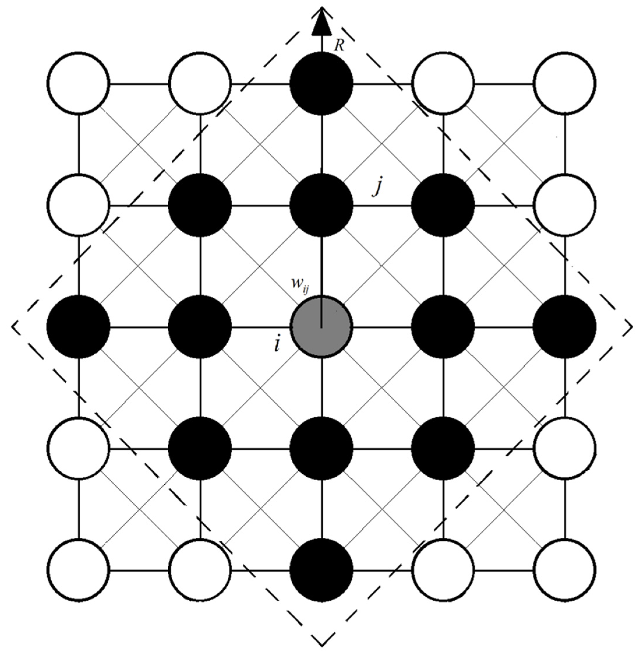
A schematic diagram of the BINN is shown in Figure 2.

4.

Path generation strategy:

The BINN planner maintains a path list, starting from the initial position. At each step,

(a)

Update the neural network: Update all neurons according to the dynamics described above.

(b)

Select the next position: From the neighborhood (distance ≤ R) of the current position $(i_c,j_c)$, select uncovered grids as candidate set $C$.

If the previous movement direction is $(\Delta i,\Delta j)$, and $(i_c+\Delta i,j_c+\Delta j)\in C$, preferentially select that grid (directional inertia).

Otherwise, select the grid with the maximum neuronal activity value in the candidate set:

$$(i_{next},j_{next})=\underset{(p,q)\in C}{\arg \max } v_{pq}$$

(13)

when multiple maxima are present, select the one with the smallest Manhattan distance.

(c)

Deadlock escape: If $C\in \phi$ (i.e., no uncovered grids in the neighborhood), invoke the A* algorithm to plan the shortest path from the current position to the “highest uncovered density” grid, and advance one step along that path (see Section 3.4).

(d)

Add the new position to the path, mark it as covered, set its external input $I$ to zero, and repeat until all designated grids are covered.

Starting from its initial point (the global center), each AUV examines all uncovered grid points within its neighborhood at each step and selects the point with the highest neuronal activity value $v$ as the next target. This “greedy” strategy ensures that the AUV always moves toward the “most attractive” direction. To promote smoother “lawnmower” paths, a heuristic rule is added: if there remains an uncovered neighbor in the previous movement direction, the AUV preferentially continues straight. When the AUV moves to a new grid point, its external input $I$ is set to zero, indicating coverage. The entire network’s neuronal activity values v are then updated through one iteration of the above equation. This “move–update” cycle continues until all grid points in the sub-region are covered.

The advantage of BINN lies in its dynamic and adaptive characteristics. By tuning parameters, it can generate smooth, low-repetition “lawnmower” paths and naturally navigate around obstacles.

3.4. A*-Based Deadlock Resolution and Path Closure

When the BINN planner detects a deadlock (no uncovered grids in the neighborhood while the sub-region is not yet fully covered), the A* algorithm is invoked. This algorithm plans the shortest path from the current position to an uncovered grid with the highest “uncovered neighbor density”. Once the deadlock is resolved, the AUV switches back to BINN mode to continue coverage.

After completing full coverage of the sub-region, the AUV’s final position typically does not coincide with the center point. The A* algorithm is invoked again to plan the optimal collision-free return path from the current position back to the center point.

4. Simulation Results and Discussion

We evaluated our architecture against four baselines in a controlled simulation environment.

4.1. Experimental Setup

All tests shared the following settings:

• Domain: $5000 \mathrm{m}\times 5000 \mathrm{m}$ square.
• Grid resolution: $200 \mathrm{m}$, resulting in a $25\times 25$ grid map.
• Obstacles: Several $2\times 2$ square blocks, generated using random seeds to ensure that obstacle positions are not fixed in each simulation.
• AUV formation: Five operational AUVs, speed $3 \mathrm{m}/\mathrm{s}$, start/end at the geometric center.
• All simulation experiments presented in this paper were conducted on a computer equipped with an AMD Ryzen 9 7945HX processor (16 cores, 32 threads, AMD (Advanced Micro Devices, Inc.), Bayan Lepas, Penang, Malaysia) and 16 GB of DDR5 RAM. The code was developed and executed in a Python 3.13 environment.

To comprehensively evaluate the performance of each algorithmic architecture, the following seven key metrics are defined:

• Maximum mission duration (s): The time of the last AUV to complete its task in the formation; the core efficiency indicator.
• Mean mission duration (s): The average mission duration across all AUVs.
• Standard deviation of mission durations (s): Measures the balance of task allocation.
• Repeat coverage rate (%): $\rho ={\displaystyle \frac{{\displaystyle {\displaystyle \sum _{k=1}^N}{N}_k^{\mathrm{cov}}}-{\displaystyle {\displaystyle \sum _{k=1}^N}{U}_k}}{{\displaystyle \sum _{k=1}^N{U}_k}}}\times 100\%$, where ${\displaystyle \sum _{k=1}^N{N}_k^{\mathrm{cov}}}$ is the total number of coverage path steps, and ${\displaystyle \sum _{k=1}^N{U}_k}$ is the total number of unique traversable grid cells that require coverage in the region. The transit paths to the mission region and the A* return paths are excluded from consideration.
• Total number of turns: Total number of turns across all AUV coverage paths (a turn is counted when two consecutive movement vectors are not parallel), likewise excluding the outbound transit and return paths.
• Algorithm runtime (s): Total computation time from region partitioning to path generation.
• Coverage rate: A fundamental metric; all architectures achieve 100%.

All experimental data presented below are averaged over at least 20 independent simulation runs.

4.2. Experimental Comparison of Baseline Algorithm Architectures

To verify the advantages and methodological novelty of the proposed framework, two independent and representative baselines are selected: DARP + Improved STC and CVT/Lloyd + Sweep CPP. DARP represents the distance-field-based iterative allocation paradigm, which iteratively balances workload through evaluation matrices and has been widely validated in multi-robot coverage. CVT/Lloyd represents the classical geometric equilibrium paradigm, where seed points are iteratively adjusted to equalize Voronoi cell areas. Improved STC represents deterministic spanning-tree coverage, while Sweep CPP represents directionally persistent lawnmower sweeps. Together, these two baselines cover the principal combinations of partitioning strategy and path generation strategy, ensuring that the comparison is not biased toward variants of the proposed framework (

Table 1. Performance comparison against baseline algorithm architectures.

Algorithm Architecture	Max Mission Duration (s)	Mean Mission Duration (s)	Std Dev of Mission Durations (s)	Repeat Coverage (%)	Total Number of Turns	Algorithm Runtime (s)
Dual-layer PSO + Voronoi + BINN (Proposed)	9325.00 ± 102.02	9199.95 ± 139.25	84.30 ± 22.84	11.26 ± 0.58	215.63 ± 11.42	476 ± 13
DARP + Improved STC	13,104.86 ± 542.55	10,754.34 ± 266.91	2539.68 ± 287.97	16.24 ± 1.83	185.38 ± 13.66	7 ± 0
CVT/Lloyd + Sweep CPP	12,443.28 ± 457.62	10,397.36 ± 204.90	1621.03 ± 263.97	15.78 ± 1.32	197.63 ± 11.88	6 ± 0

).

TSP formulates coverage as discrete point-to-point routing, which is categorically different from continuous area sweeping; for an underactuated AUV with side-scan sonar, a TSP-derived path produces discontinuous, sharp-turning trajectories that break sensor swath continuity and cause unrecoverable data gaps. Therefore, TSP is retained only as an illustrative counterexample rather than a competitive baseline.

The following figures present the experimental results.

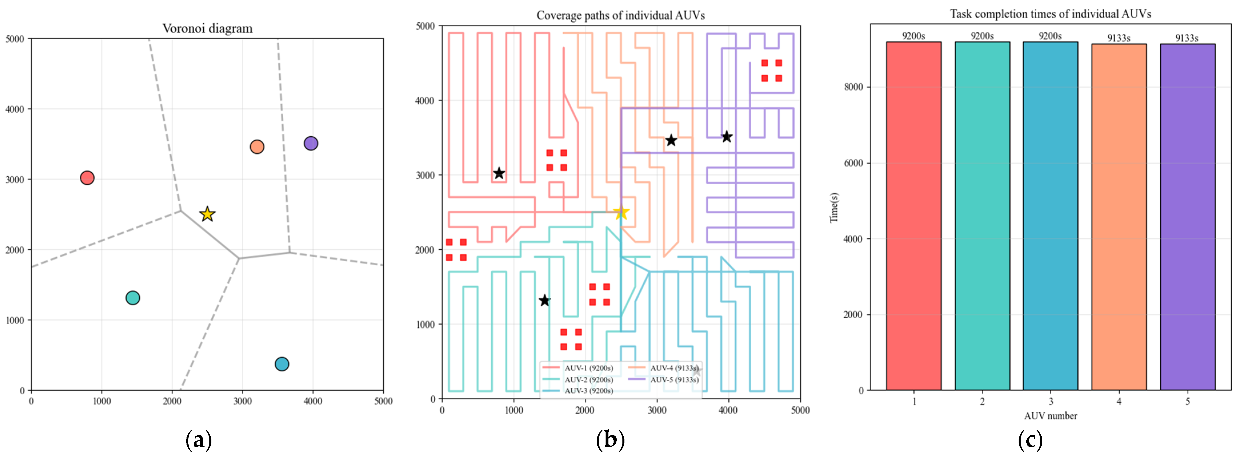
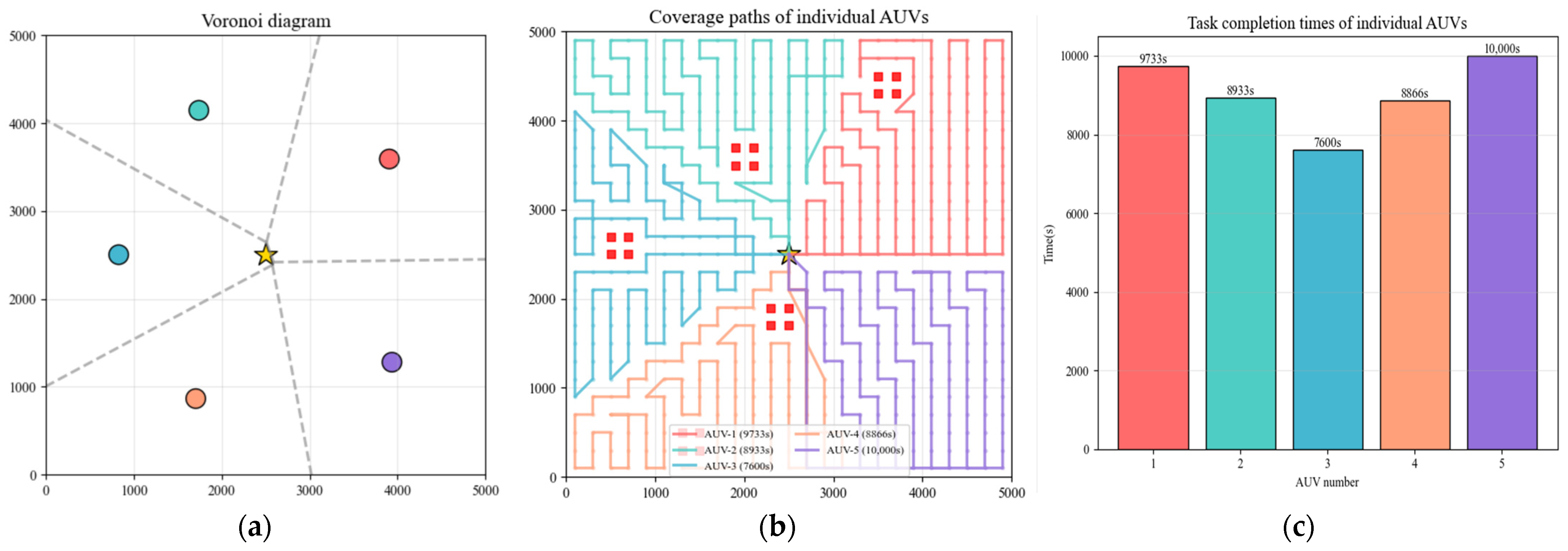
• Dual-layer PSO + Voronoi + BINN (Proposed): The architecture described in Section 3. Simulation results are presented in Figure 3.

2.

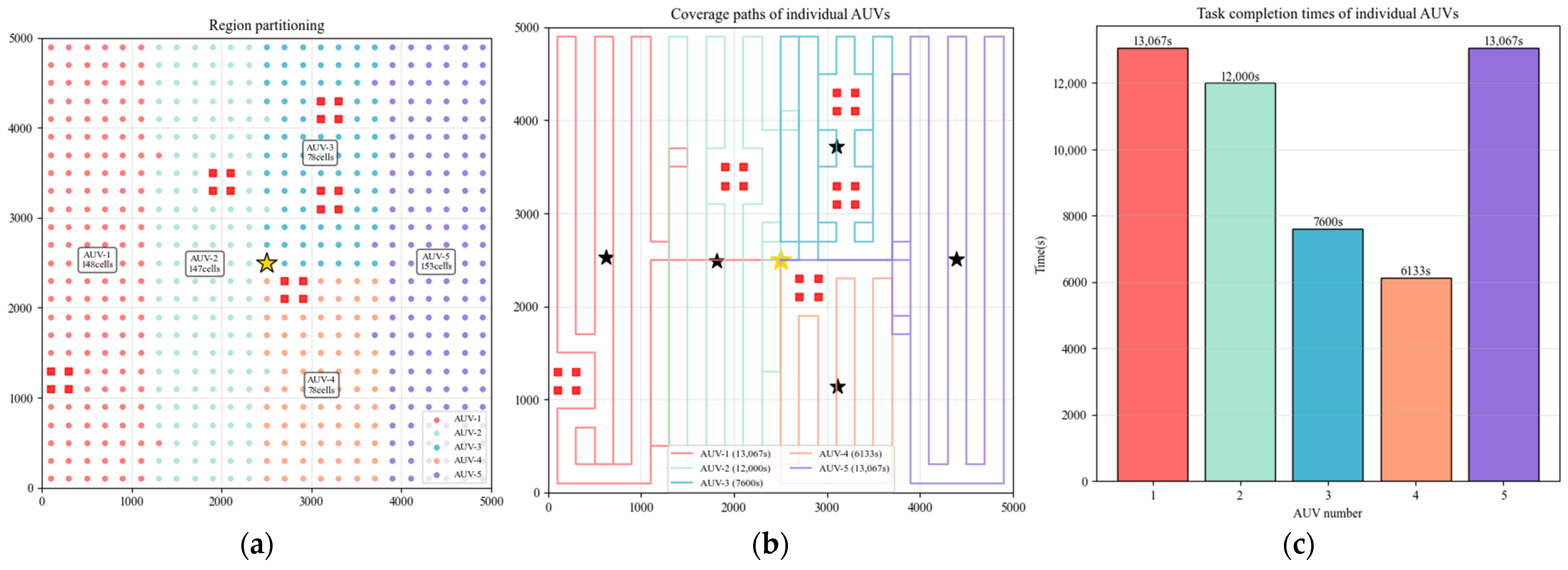
DARP + Improved STC: DARP for balanced partitioning and improved STC for subsequent coverage path planning. Simulation results are shown in Figure 4.

3.

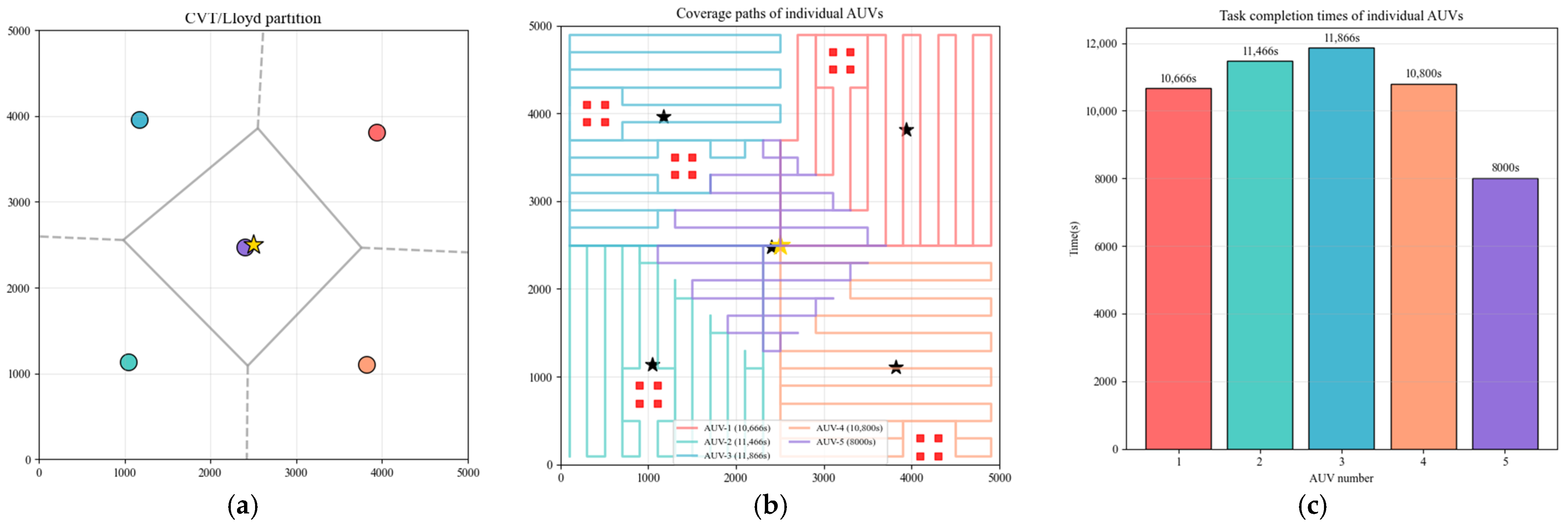
CVT/Lloyd + Sweep CPP: CVT/Lloyd for balanced partitioning and sweep CPP for subsequent coverage path planning. Simulation results are shown in Figure 5.

The data presented in Table 1 are analyzed as follows. The proposed architecture achieves the lowest maximum mission duration. Its standard deviation of mission durations is lower than those of DARP + Improved STC and CVT/Lloyd + Sweep CPP by factors of 30.1 and 19.2, respectively. This confirms that temporal load balancing cannot be achieved by geometric equilibrium alone: both baselines produce spatially balanced partitions, yet their mission-time dispersion remains more than an order of magnitude larger. The reason is that neither incorporates the actual traversal time of the coverage path into the partitioning objective. The proposed method directly minimizes the BINN-simulated makespan and time variance, reshaping Voronoi seeds to absorb the nonlinear path cost caused by different obstacle configurations and varying sub-region distances. This comparison directly demonstrates that, in this scenario, temporal balancing is superior to area balancing as the workload unit for multi-AUV coverage operations. In terms of path quality, the proposed method achieves a repeat coverage rate of 11.26%, outperforming DARP + Improved STC and CVT/Lloyd + Sweep CPP in this metric. Its turn count is approximately 215, slightly higher than those of the two baselines, but this modest increase in steering effort is justified by the lower repeat coverage rate. The runtime of the proposed method (476 s) is longer, but as discussed in Section 3.2.3, this overhead is acceptable for offline strategic planning.

4.3. Ablation Study

To isolate the contribution of each component in the proposed framework, four ablation variants are evaluated. All variants share the same BINN-based path generator and differ only in their partitioning strategy (

Table 2. Ablation study results.

Algorithm Architecture	Max Mission Duration (s)	Mean Mission Duration (s)	Std Dev of Mission Durations (s)	Repeat Coverage (%)	Algorithm Runtime (s)
Dual-layer PSO + Voronoi + BINN (Proposed)	9325.00 ± 112.88	9199.95 ± 129.25	84.30 ± 22.84	11.26 ± 0.72	476 ± 15
Single-layer PSO + Voronoi + BINN	10,091.28 ± 436.22	9426.67 ± 125.48	473.50 ± 104.33	14.88 ± 1.16	18 ± 2
Random-seed second-layer PSO + Voronoi + BINN	10,136.43 ± 266.39	9632.73 ± 178.01	203.61 ± 45.20	15.26 ± 1.13	519 ± 16
Sector Uniform Partitioning + BINN	10,316.68 ± 481.61	9233.33 ± 105.41	873.23 ± 172.97	13.08 ± 0.88	12 ± 1

).

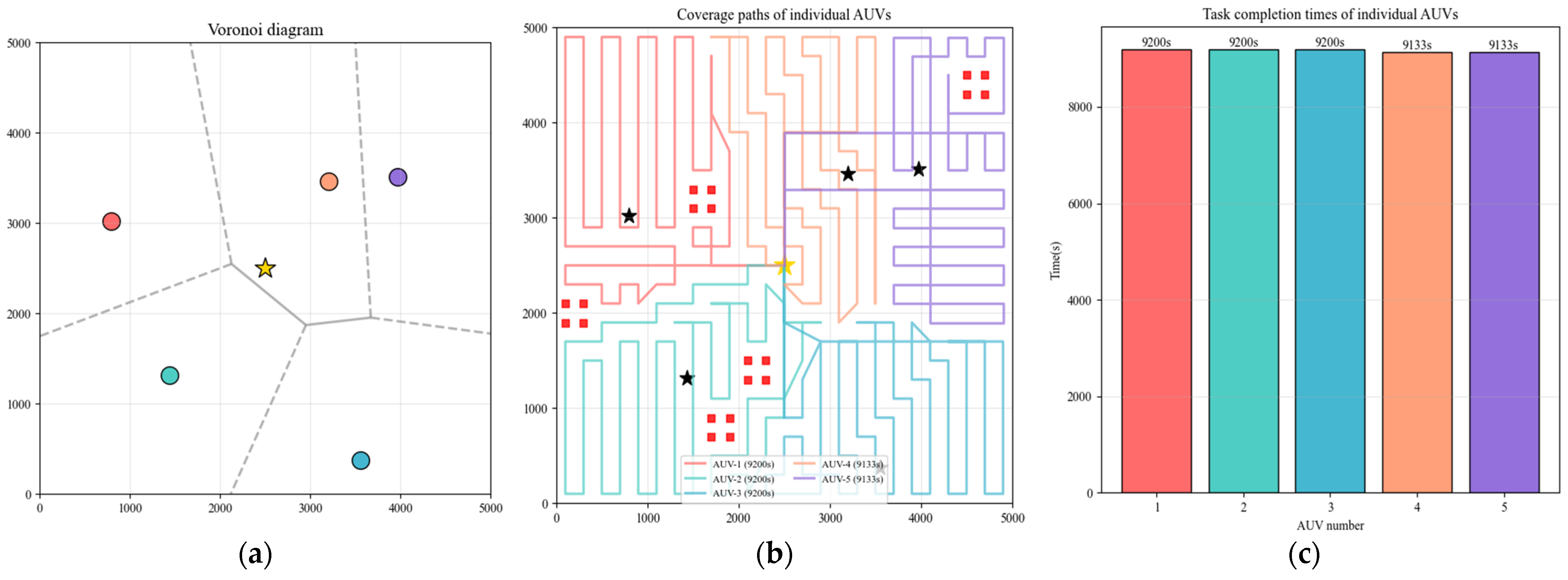
• Dual-layer PSO + Voronoi + BINN (Proposed): Simulation results are presented in Figure 6.

2.

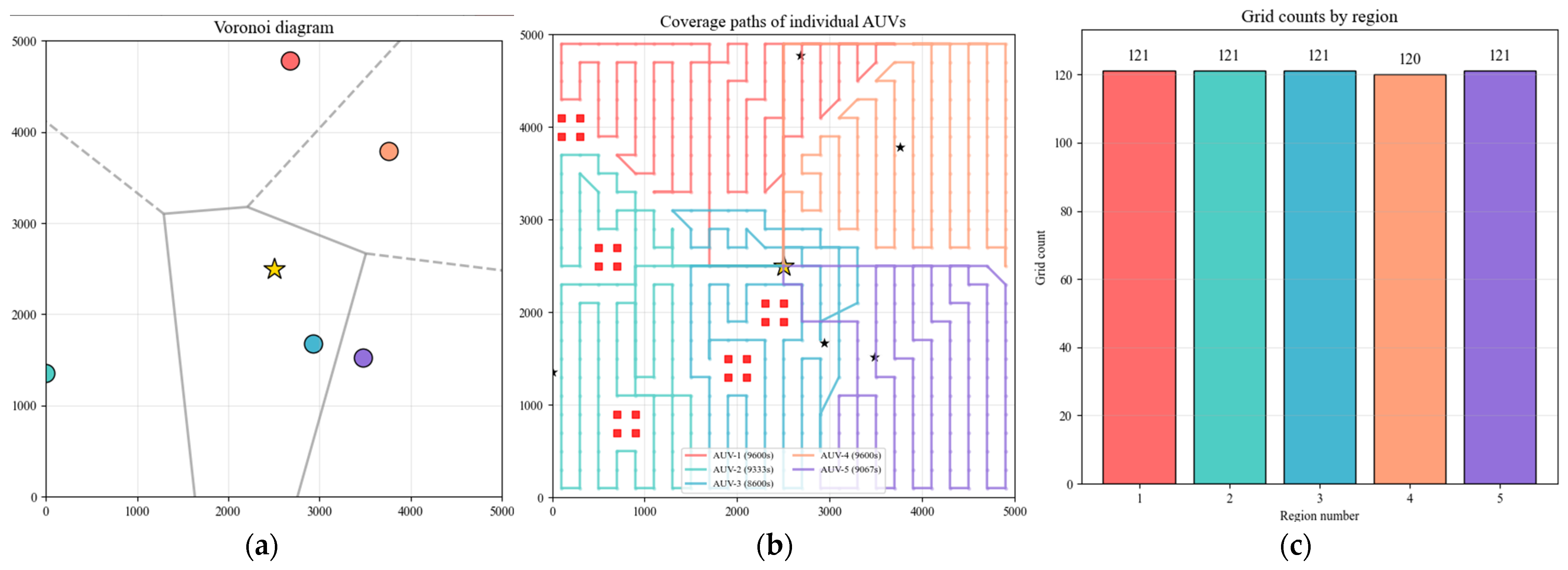
Single-layer PSO + Voronoi + BINN: Only the first-layer PSO (area balancing) is executed, followed by BINN planning. Simulation results are shown in Figure 7.

3.

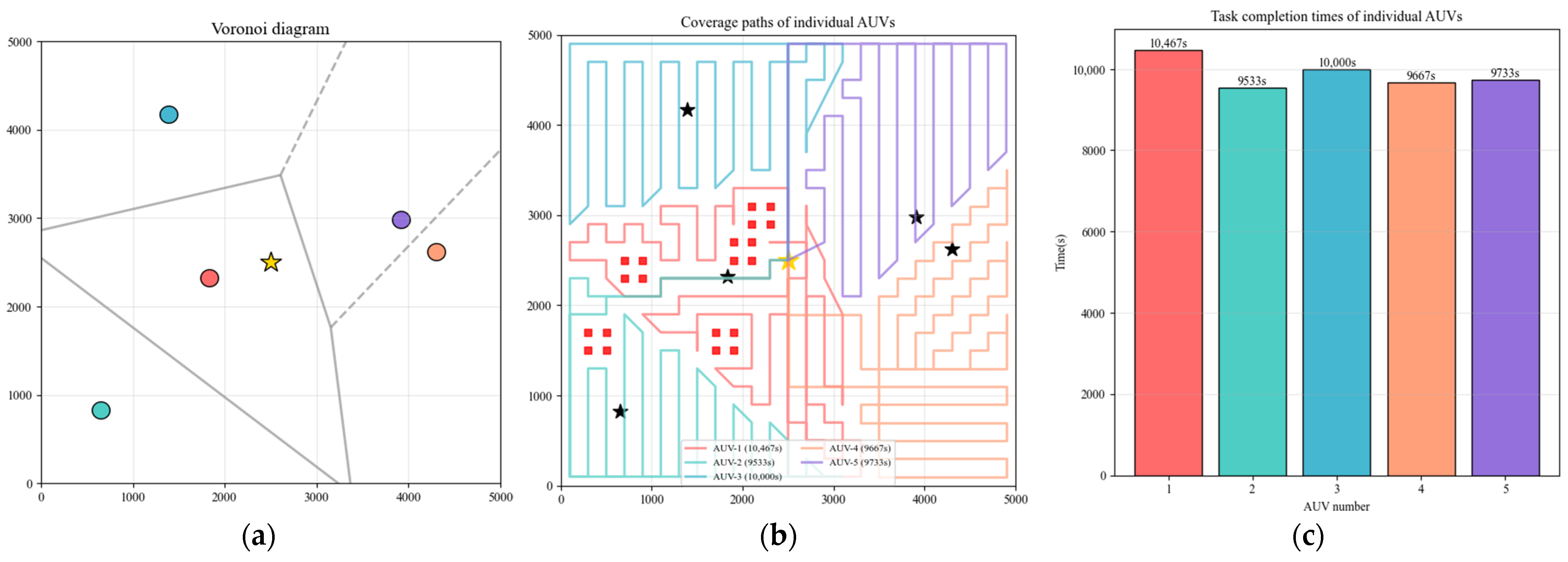
Random-seed second-layer PSO + Voronoi + BINN: The coarse partitioning from the first-layer PSO is replaced with random Voronoi seed points, and only the second-layer PSO is employed. Simulation results are presented in Figure 8.

4.

Sector Uniform Partitioning + BINN: The entire region is uniformly divided from the center point by angles of 360/N degrees, followed by BINN planning. Simulation results are presented in Figure 9.

The data presented in Table 2 are analyzed as follows. Comparing full against single-layer PSO reveals the value of directly optimizing temporal balance: single-layer PSO reduces grid-count variance to near-zero, yet its mission-time standard deviation remains 473.50 s—more than five times as large as that of the full framework. The second-layer PSO absorbs the nonlinear time inflation caused by obstacle topology and varying sub-region distances, compressing the idle gap from 473.50 s to 84.30 s. Comparing the full method against the random-seed second-layer PSO isolates the value of the first-layer coarse initialization: with random-seed initialization, the second-layer PSO still reduces time dispersion to 203.61 s, which is more than twice the dispersion of the full framework (84.30 s). Furthermore, due to the absence of the first-layer coarse initialization, the optimization time of the second-layer PSO increases slightly, exceeding the algorithm runtime of the full framework by about 10%. Comparing full against geometric Voronoi partition shows the combined effect of both PSO layers: pure geometric partitioning yields a standard deviation of 873.23 s, an order of magnitude worse. This confirms that the nested PSO architecture—not any single component—is responsible for the dramatic improvement in temporal load balancing.

4.4. Comparative Experiments Under Varying Obstacle Densities and Fleet Sizes

To verify that the advantages of the proposed framework are not coincidental to a specific obstacle distribution and to evaluate its scalability, two groups of comparative experiments are conducted. The first group tests three obstacle density levels: the original density, +100% density, and +150% density, while other settings remain unchanged. The second group tests three fleet sizes: $N=3,5,7$ AUVs, while other settings remain unchanged. Each configuration above is averaged over 20 independent runs.

Table 3. Performance under different configurations.

Algorithm Architecture	Performance Metrics	Obstacle Density 1 (Original)	Obstacle Density 1 (+100%)	Obstacle Density 1 (+200%)	Fleet Size 1 (N = 3)	Fleet Size 2 (Original N = 5)	Fleet Size 3 (N = 7)
Dual-layer PSO + Voronoi + BINN (Proposed)	Max Mission Duration (s)	9325.00 ± 112.88	9320.93 ± 113.69	9289.36 ± 109.56	14,518 ± 357.65	9325.00 ± 112.88	7194.22 ± 105.97
	Std Dev of Mission Durations (s)	84.30 ± 22.84	81.49 ± 26.82	127.95 ± 36.01	31.43 ± 9.72	84.30 ± 22.84	60.21 ± 15.03
	Algorithm Runtime (s)	476 ± 15	472 ± 16	483 ± 18	403 ± 13	476 ± 15	493 ± 18
DARP + Improved STC	Max Mission Duration (s)	13,104.86 ± 542.55	14,148.11 ± 482.83	13,837.03 ± 845.34	18,424.25 ± 727.41	13,104.86 ± 542.55	9345.44 ± 364.91
	Std Dev of Mission Durations (s)	2539.68 ± 287.97	2827.09 ± 208.64	2657.09 ± 271.66	1399.79 ± 284.48	2539.68 ± 287.97	916.44 ± 211.95
	Algorithm Runtime (s)	7 ± 0	7 ± 0	7 ± 0	7 ± 0	7 ± 0	7 ± 0
CVT/Lloyd + Sweep CPP	Max Mission Duration (s)	12,443.28 ± 457.62	12,703.04 ± 523.56	12,836.36 ± 713.29	23,648.49 ± 1306.77	12,443.28 ± 457.62	11,377.76 ± 557.78
	Std Dev of Mission Durations (s)	1621.03 ± 263.97	1507.42 ± 222.81	1454.52 ± 286.29	4674.52 ± 790.63	1621.03 ± 263.97	1582.66 ± 253.51
	Algorithm Runtime (s)	6 ± 0	6 ± 0	6 ± 0	6 ± 0	6 ± 0	6 ± 0

presents the data comparison of the three algorithm architectures under different configurations.

Under three obstacle density levels, the proposed framework consistently achieves the lowest time dispersion and the shortest makespan, with its relative advantage remaining stable. At a 200% increase in obstacle density, the standard deviation of the proposed method (81.49 s) is approximately one-thirtieth of that of DARP + Improved STC (2657.09 s) and approximately one-twentieth of that of CVT/Lloyd + Sweep (1454.52 s). This confirms that the nonlinear time inflation caused by obstacle topology is precisely what the second-layer PSO is designed to absorb, and that its effectiveness does not depend on a particular obstacle configuration. Across underwater terrains of varying complexity, it consistently achieves an approximately one order of magnitude lower time standard deviation.

As fleet size increases from 3 to 7, the makespan decreases for all methods. The proposed method maintains the lowest time dispersion across all fleet sizes: at $N=7$, its standard deviation (60.21 s) is approximately one-fifteenth of that of DARP + STC (916.44 s) and less than one-twentieth of that of CVT/Lloyd + Sweep (1582.66 s), i.e., more than an order of magnitude lower. This demonstrates that the temporal balancing advantage of the proposed method is scale-invariant and scalable: it does not degrade as the fleet grows, and it consistently achieves temporal balancing across commonly used AUV fleet sizes. Runtime grows with fleet size, reflecting the increased number of BINN path planning runs, but remains acceptable for offline planning.

4.5. Discussion

4.5.1. Relationship Between Path Planning and Practical Execution

The path planning developed in this study operates at the strategic level: given a static, pre-surveyed environment, it generates a discrete sequence of waypoints that guarantees full coverage while minimizing makespan and turn counts. In practice, however, the planned path may deviate from the intended trajectory due to vehicle dynamics, ocean currents, and localization errors. Hence, path planning and trajectory execution must be conceptually distinguished yet systematically coordinated.

This issue has been extensively discussed in the literature. Borja-Jaimes et al. [30] proposed a robust tracking framework for underactuated vehicles, combining backstepping sliding mode control with a super-twisting observer that reconstructs velocities and rejects bounded disturbances using only position and attitude measurements, thereby ensuring closed-loop tracking accuracy. Their work implies that without a robust low-level controller, the kinematic feasibility claimed at the planning stage is unlikely to hold in real underwater environments. Conversely, Li et al. [31] addressed the coupling from the planning side by explicitly incorporating current-aware path tracking into their ER-MCPP algorithm, emphasizing that environmental disturbances should be anticipated during planning rather than treated as an afterthought.

In this paper, we adopt a decoupled planning–execution architecture, focusing on coverage path planning for static, pre-surveyed scenarios, with the goal of generating waypoint sequences for each AUV that achieve full coverage and temporal load balancing. The effects of AUV dynamics, tracking performance, and environmental disturbances on trajectory execution are beyond the scope of this study. The rationale for this separation is that the planning layer can concentrate on coverage combinatorial optimization—a problem dominated by combinatorial complexity—while the robustness of the execution layer can be independently ensured by existing control frameworks. Under this layered logic, the feasibility assessment of planning solutions is based on kinematic-level waypoint sequences, while actual tracking accuracy depends on the performance of the low-level controller. Future work will further investigate how AUV dynamics, tracking performance, and ocean currents affect the execution of planned trajectories, aiming for tighter integration between planning and control.

4.5.2. Summary of Findings

The experimental results of this study collectively demonstrate three key findings:

• Temporal load balancing cannot be achieved by geometric equilibrium alone. Both DARP and CVT/Lloyd produce spatially balanced partitions, yet their mission-time dispersion remains an order of magnitude larger than that of the proposed method. This confirms that time, not area, is the correct workload unit for multi-AUV coverage operations.
• The nested PSO architecture is responsible for the improvement. The ablation study shows that neither the first-layer coarse balancing nor the second-layer temporal optimization alone can match the full framework. The first layer provides a high-quality starting point; the second layer absorbs the nonlinear path cost. Together, they reduce time dispersion by an order of magnitude relative to geometric partitioning.
• The advantage is robust and scalable. The obstacle-density experiments confirm that the framework’s advantage is not an artifact of a specific obstacle distribution, and the fleet-size experiments confirm that it does not degrade as the number of AUVs grows.

4.5.3. Operational Boundary and Computational Trade-Off

The proposed architecture is strictly prescribed for strategic, offline, static-environment deployments. In such scenarios, the 8 min offline preprocessing is a justifiable one-time investment: it amortizes over a 3 h field mission (about 5% of the total timeline) and enables near-synchronous formation completion, which is critical for eliminating the idle energy waste of early-completing AUVs and preventing mission failure due to insufficient energy for lagging AUVs. This confirms that for the static underwater environments with irregular obstacles studied in this paper, temporal load balancing avoids the pitfall of uneven time workload caused by equal-area division and provides a more operationally relevant workload metric for multi-AUV coverage tasks. Complementing this, BINN’s directional inertia ensures smooth, lawnmower-style sweeps, circumventing the excessive turns of TSP-style routing. Crucially, all computation is performed on shore-based servers and the mother AUV, rather than on the operational AUVs; waypoint sequences are uploaded prior to the mission, requiring only minimal execution-time computation. The framework is not recommended for highly dynamic environments or scenarios demanding rapid online re-planning. Its main limitation is the computational overhead, which scales with grid resolution and fleet size. Future work will investigate surrogate-model acceleration to relax this boundary and integrate explicit energy consumption models and ocean current disturbances into the partitioning objective.

5. Conclusions

This paper demonstrates that for static underwater environments with irregular obstacles, temporal load balancing—specifically, minimizing the idle waiting time of early-finishing vehicles—avoids the pitfall of uneven time workload caused by equal area division, and provides a more operationally relevant workload metric for multi-AUV coverage missions compared with traditional spatial area balancing. By introducing a dual-layer nested PSO framework, we bridge the gap between static Voronoi partitioning and dynamic path execution, directly optimizing the actual makespan derived from BINN-generated sweeps. Experiments demonstrate that this PSO nesting strategy reduces the standard deviation of makespans by an order of magnitude. The methodological novelty of this work lies not in the individual techniques—Voronoi partitioning, PSO, and BINN are well established—but in the nested coupling architecture that renders the partitioning process responsive to the nonlinear, topology-dependent time costs of coverage sweeps. Existing time-balancing methods typically optimize partitioning under a cost model that is either spatially geometric or analytically approximated. By embedding a path-simulation-based time cost directly into the inner optimization loop, this work demonstrates a fundamentally different—and more effective—load-balancing behavior, reducing time standard deviation by an order of magnitude relative to single-layer geometric optimization. The core objective of this temporal balancing design is to eliminate idle energy waste of early-completing AUVs and prevent mission failure caused by insufficient endurance of lagging AUVs, thus improving the overall energy utilization efficiency of the formation. It should be noted that the energy efficiency improvement is a derived conclusion based on typical AUV power characteristics, rather than a direct measurement from simulations. Furthermore, we have provided a categorical refutation of TSP-based routing for continuous underwater surveying, clarifying that discrete point-hopping trajectories are kinematically and sensorially incompatible with AUV operations. We emphasize that these conclusions are validated at the mission planning level. Practical deployment would require post-processing of trajectories to satisfy AUV turning radius and vehicle dynamics constraints. However, this does not alter the relative superiority of temporal balancing over spatial partitioning. The proposed architecture is strictly prescribed for strategic, offline, static-environment deployments, where an 8 min computational overhead is a justifiable trade-off for near-synchronous formation completion. Future work will extend this study in two directions. First, surrogate-model acceleration will be investigated to reduce the computational cost of the nested optimization framework and support faster re-planning, thereby relaxing the offline planning boundary and enabling adaptive re-planning against mild environmental perturbations. Second, explicit energy consumption models and ocean current disturbances will be integrated into the partitioning objective to achieve joint temporal-energy load balancing for more realistic operational scenarios.

6. Patents

Ke, Y.S.; Wang, N.; Gao, X.P.; Huo, C.; Xu, M.J.; Ye, Q. A Collaborative Coverage Planning Method and System for Multi-Autonomous Underwater Vehicles. Chinese Patent Application No. 202611034087.3, filed 13 July 2026 (pending).

References

1. Gong, J.; Kim, H.; Lee, S. Resilient multi-robot coverage path redistribution using boustrophedon decomposition for environmental monitoring. Sensors 2024, 24, 7482. [Google Scholar] [CrossRef] [Scilit] [PubMed]
2. Cortés, J.; Martínez, S.; Karatas, T.; Bullo, F. Coverage control for mobile sensing networks. IEEE Trans. Robot. Autom. 2004, 20, 243–255. [Google Scholar] [CrossRef] [Scilit]
3. Hungerford, K.; Dasgupta, P.; Guruprasad, K.R. A repartitioning algorithm to guarantee complete, non-overlapping planar coverage with multiple robots. In Proceedings of the 12th International Symposium on Distributed Autonomous Robotic Systems; Springer Tracts in Advanced Robotics; Springer: Berlin/Heidelberg, Germany, 2014; Volume 112, pp. 33–48. [Google Scholar]
4. Sadek, M.G.; El-Garhy, A.M.; Mohamed, A.E. A dynamic cooperative multi-agent online coverage path planning algorithm. In Proceedings of the 2021 16th International Conference on Computer Engineering and Systems (ICCES), Cairo, Egypt, 15–16 December 2021; IEEE: New York, NY, USA, 2021; pp. 1–9. [Google Scholar]
5. Kapanoglu, M.; Alikalfa, M.; Ozkan, M.; Yazici, A.; Parlaktuna, O. A pattern-based genetic algorithm for multi-robot coverage path planning minimizing completion time. J. Intell. Manuf. 2012, 23, 1035–1045. [Google Scholar] [CrossRef] [Scilit]
6. Ni, J.; Gu, Y.; Tang, G.; Ke, C.; Gu, Y. Cooperative coverage path planning for multi-mobile robots based on improved k-means clustering and deep reinforcement learning. Electronics 2024, 13, 944. [Google Scholar] [CrossRef] [Scilit]
7. Cai, S.J.; Yan, Z.P.; Hou, S.P.; Li, J.X. A rolling planning method for Multi-UUV cooperative area detection and patrol. Ocean. Eng. 2026, 358, 125571. [Google Scholar] [CrossRef] [Scilit]
8. Li, Y.; Juan, R.; Zhou, Y.; Wang, T.; Li, Z.; Guo, W.; Gao, Z. AD-RRT*: An RRT*-based global path planning approach for underwater gliders with alpha shapes and DBSCAN. Expert Syst. Appl. 2025, 291, 128219. [Google Scholar] [CrossRef] [Scilit]
9. Shao, Z.; Moon, Y.B.; Yang, Y.C.; Kumral, M. Underground Haulage Network Design Using HDBSCAN and RRT Algorithms Built on Dubins Path. Min. Metall. Explor. 2023, 40, 773–786. [Google Scholar] [CrossRef] [Scilit]
10. Xue, J.; Tian, J.; Wang, J. Multi-agent reinforcement learning for area coverage in unknown environments. J. Phys. Conf. Ser. 2025, 3072, 012003. [Google Scholar] [CrossRef] [Scilit]
11. Zhou, Y.; Xiao, J.; Zhou, Y.; Loianno, G. Multi-robot collaborative perception with graph neural networks. IEEE Robot. Autom. Lett. 2022, 7, 2289–2296. [Google Scholar] [CrossRef] [Scilit]
12. Li, Y.; Li, L.; Xiong, S.; Ma, M.; Yan, Y.; Meng, Y.; Jin, H. Game-based coverage path planning for multiple Dubins robots in agricultural fields. Robotica 2026, 1–24. [Google Scholar] [CrossRef] [Scilit]
13. KrisshnaKumar, P.; Witter, J.; Collins, L.; Pothuri, J.P.K.V.; Ghassemi, P.; Esfahani, E.T.; Dantu, K.; Chowdhury, S. Efficient planning for scalable and load-balanced area coverage by multiple unmanned aerial vehicles. J. Comput. Inf. Sci. Eng. 2026, 26, 091002. [Google Scholar] [CrossRef] [Scilit]
14. Kim, K.; Kim, J. Efficient graph-based area partitioning for balanced multi-robot coverage path planning. Robot. Auton. Syst. 2026, 201, 105445. [Google Scholar] [CrossRef] [Scilit]
15. Gu, M.; Song, Y.; Ra, C.; Suk, J.; Oh, H. Iterative task decomposition and allocation for fixed-wing multi-UAV coverage path planning. Int. J. Aeronaut. Space Sci. 2026, 27, 774–790. [Google Scholar] [CrossRef] [Scilit]
16. Galceran, E.; Carreras, M. A survey on coverage path planning for robotics. Robot. Auton. Syst. 2013, 61, 1258–1276. [Google Scholar] [CrossRef] [Scilit]
17. Al-Kaff, A.; Martín, D.; García, F.; de la Escalera, A.; Armingol, J.M. Coverage path planning methods focusing on energy efficient and cooperative strategies for unmanned aerial vehicles. Sensors 2022, 22, 1235. [Google Scholar] [CrossRef] [Scilit] [PubMed]
18. Kapoutsis, A.C.; Chatzichristofis, S.A.; Kosmatopoulos, E.B. DARP: Divide areas algorithm for optimal multi-robot coverage path planning. J. Intell. Robot. Syst. 2017, 86, 663–680. [Google Scholar] [CrossRef] [Scilit]
19. Galceran, E.; Carreras, M. Efficient seabed coverage path planning for ASVs and AUVs. In Proceedings of the 2012 IEEE/RSJ International Conference on Intelligent Robots and Systems, Vilamoura-Algarve, Portugal, 7–12 October 2012; IEEE: New York, NY, USA, 2012; pp. 88–93. [Google Scholar]
20. Bagnitckii, A.; Inzartsev, A.; Pavin, A. Planning and correction of the AUV coverage path in real time. In Proceedings of the 2017 IEEE Underwater Technology (UT), Busan, South Korea, 21–24 February 2017; IEEE: New York, NY, USA, 2017; pp. 1–6. [Google Scholar]
21. Akopov, A.S.; Beklaryan, L.A.; Beklaryan, A.L. Cluster-Based Optimization of an Evacuation Process Using a Parallel Bi-Objective Real-Coded Genetic Algorithm. Cybern. Inf. Technol. 2020, 20, 45–63. [Google Scholar] [CrossRef] [Scilit]
22. Meng, Z.; Lin, F.; Lin, X. Q-learning Based Differential Evolution with Mutation Strategy Selection for 3D Uncrewed Aerial Vehicle Path Planning. Inf. Sci. 2026, 756, 123839. [Google Scholar] [CrossRef] [Scilit]
23. Chen, G.Z.; Shen, Y.; Duan, X.Y.; Wan, J.; Yan, T.; He, B. Coverage path planning based on improved exact cellular decomposition method in ocean survey. In Proceedings of the Global Oceans 2020, Biloxi, MS, USA, 5–30 October 2020; IEEE: New York, NY, USA, 2020; pp. 1–4. [Google Scholar]
24. Chen, Z.; Gao, J.; Ma, J.; Wang, X. A 3D adaptive spiral coverage path planning algorithm of autonomous underwater vehicle for enhanced edge-corner coverage. Meas. Sci. Technol. 2025, 36, 076309. [Google Scholar] [CrossRef] [Scilit]
25. Zhu, D.; Zhu, T.; Yan, M. Multi-AUV complete coverage path planning based on improved neural network. J. Syst. Simul. 2020, 32, 1505–1514. (In Chinese) [Google Scholar] [CrossRef]
26. Luna, M.A.; Molina, M.; Da-Silva Gomez, R.; Melero-Deza, J.; Arias-Perez, P.; Campoy, P. A multi-UAV system for coverage path planning applications with in-flight re-planning capabilities. J. Field Robot. 2024, 41, 1480–1497. [Google Scholar] [CrossRef] [Scilit]
27. Aurenhammer, F. Voronoi diagrams—A survey of a fundamental geometric data structure. ACM Comput. Surv. 1991, 23, 345–405. [Google Scholar] [CrossRef] [Scilit]
28. Kennedy, J.; Eberhart, R. Particle swarm optimization. In Proceedings of the 1995 International Conference on Neural Networks (ICNN’95), Perth, Australia, 27 November–1 December 1995; IEEE: New York, NY, USA, 1995; pp. 1942–1948. [Google Scholar]
29. Cai, W.; Zhang, S.; Zhang, M.; Wang, C. Improved BINN-Based Underwater Topography Scanning Coverage Path Planning for AUV in Internet of Underwater Things. IEEE Internet Things J. 2023, 10, 18375–18386. [Google Scholar] [CrossRef] [Scilit]
30. Borja-Jaimes, V.; García-Morales, J.; Escobar-Jiménez, R.F.; Guerrero-Ramírez, G.V.; Adam-Medina, M. A Backstepping Sliding Mode Control of a Quadrotor UAV Using a Super-Twisting Observer. Appl. Sci. 2025, 15, 10120. [Google Scholar] [CrossRef] [Scilit]
31. Li, L.; Li, Y.; Wang, Y.; Xu, G.; Wang, H.; Gao, P.; Feng, X. Multi-AUV Coverage Path Planning Algorithm Using Side-Scan Sonar for Maritime Search. Ocean. Eng. 2024, 300, 117396. [Google Scholar] [CrossRef] [Scilit]
Figure 1. Algorithm architecture flowchart.
Applsci 16 09300 g001
Figure 2. Schematic diagram of the BINN.
Applsci 16 09300 g002
Figure 3. (a) Region partitioning map. (b) Coverage paths of individual AUVs. (c) Task completion time histogram of individual AUVs.
Applsci 16 09300 g003
Figure 4. (a) Region partitioning map. (b) Coverage paths of individual AUVs. (c) Task completion time histogram of individual AUVs.
Applsci 16 09300 g004
Figure 5. (a) Region partitioning map. (b) Coverage paths of individual AUVs. (c) Task completion time histogram of individual AUVs.
Applsci 16 09300 g005
Figure 6. (a) Region partitioning map. (b) Coverage paths of individual AUVs. (c) Task completion time histogram of individual AUVs.
Applsci 16 09300 g006
Figure 7. (a) Region partitioning map. (b) Coverage paths of individual AUVs. (c) Grid count histogram by region.
Applsci 16 09300 g007
Figure 8. (a) Region partitioning map. (b) Coverage paths of individual AUVs. (c) Task completion time histogram of individual AUVs.
Applsci 16 09300 g008
Figure 9. (a) Region partitioning map. (b) Coverage paths of individual AUVs. (c) Task completion time histogram of individual AUVs.
Applsci 16 09300 g009