A Reduced-Order Equivalent-Dipole Model for DC Stray Magnetic Fields

Abstract

Accurate characterization of stray magnetic fields is essential in high-field devices, where external fields may affect diagnostics and personnel safety. Although finite-element models provide high-fidelity solutions, they may require extensive preprocessing and discretization of large source-free regions, making repeated evaluations costly when the magnetic source is unchanged. This paper proposes a reduced-order equivalent-dipole model that provides an analytical representation of the three-dimensional background stray field after one-time offline calibration. Dipoles are placed at Gauss–Legendre nodes within an auxiliary volume, while symmetry and anti-symmetry conditions are embedded in the source mapping. Their effective moments are identified from magnetic-flux-density data through a regularized linear inverse problem. The method is assessed for the SHiP spectrometer magnet at CERN against a high-fidelity finite-element reference. A controlled comparison of five model orders selects the 125-dipole configuration, reducing the relative vector $L^2$ error on a common three-dimensional evaluation grid from 21.2% for 27 dipoles to 4.59%. An independently generated dense three-dimensional post-selection dataset confirms the accuracy of the selected model, giving a relative vector $L^2$ error of $1.77\%$ for $d_{\mathrm{aux}}\ge 0.50$ m. The complementary dense mid-plane assessment gives $0.95\%$ over the same validity region.

1. Introduction

Accurate prediction and reconstruction of DC stray magnetic fields are essential in the design, commissioning, and operation of large magnetic systems. External fields may perturb nearby diagnostics, magnetic sensors, detector electronics, and other field-sensitive equipment. In fusion devices, for example, they can also affect the transport of charged particles within diagnostic systems [1]. In addition, magnetic installations may be subject to occupational-exposure requirements and facility-specific safety rules [2,3,4,5]. A representative example is the dipole magnet developed for the Scattering and Neutrino Detector of the SHiP (Search for Hidden Particles) experiment at CERN, which is required to produce a magnetic flux density above $1.2\mathrm{T}$ over a large instrumented volume while maintaining a very low field in the surrounding region [6]. These requirements make the accurate and computationally efficient evaluation of the external field an important part of the magnet-design workflow.

Magnetostatic numerical analyses are commonly performed by means of the finite-element method (FEM), finite-difference schemes, boundary-element methods (BEM), or coupled formulations. FEM is particularly effective for complex geometries and nonlinear ferromagnetic materials. However, the treatment of an unbounded exterior domain requires either a sufficiently large truncated air region, special infinite-domain elements, or a coupling with an exterior-field formulation. Several advanced approaches have been developed to reduce this burden, including infinite-domain finite elements and FEM–BEM or FEM–Green couplings [7,8]. Consequently, the motivation for reduced field models is not that full-order methods are intrinsically unsuitable, but that repeated design iterations, dense three-dimensional field maps, uncertainty studies, and real-time or near-real-time evaluations may remain computationally expensive even when an efficient full-order formulation is available.

In a homogeneous source-free region, the magnetostatic field satisfies Maxwell’s equations and can be represented through harmonic scalar or vector potentials. This structure has motivated several physics-consistent field-reconstruction techniques. For accelerator magnets, BEM formulations have been used to reconstruct two-dimensional field maps from measured boundary data, avoiding nonphysical artifacts that may arise from direct interpolation [9] in regions such as the surrounding air, where conventional FE or FD approaches may employ relatively coarse meshes. More recently, local three-dimensional field representations derived from solutions of Laplace’s equation have been identified from distributed rotating-coil measurements through Bayesian inversion, thereby incorporating regularization and providing a route toward uncertainty quantification [10]. These studies show that a compact field representation can complement full-order simulation when the quantity of interest is the field in a prescribed source-free region rather than the complete internal electromagnetic state of the device.

A related family of techniques is based on equivalent or auxiliary sources. In the Method of Auxiliary Sources and in the closely related Method of Fundamental Solutions, the unknown field is approximated by a weighted superposition of elementary solutions whose singularities are placed outside the region in which the field is evaluated [11,12,13]. Such representations satisfy the governing differential equation exactly away from the auxiliary sources and provide inexpensive field evaluation once the source amplitudes have been determined [14]. Their numerical performance, however, depends strongly on source placement, sampling geometry, and regularization: the resulting matrices are generally dense and may be severely ill-conditioned [15,16]. The same issue arises in inverse magnetostatic identification from external field measurements, for which truncated singular-value decomposition, Tikhonov-type methods, and related regularization strategies are commonly required [17]. Therefore, the positivity of a quadrature rule or the analytical form of the elementary field does not, by itself, guarantee stability of the associated inverse problem.

For configurations that also include ferromagnetic materials, reduced source representations have been formulated in terms of equivalent currents, uniformly magnetized prisms, and magnetic dipoles. Analytical brick and dipole models have been investigated for the efficient evaluation of the contribution of ferromagnetic components in tokamaks [18], while equivalent-current formulations, also reported as stick models [19,20], have been proposed for rapid field computation in inductors and permanent magnets [21] and even to mimic the plasma behavior in a tokamak [22]. Accordingly, the methodological contribution of the present work does not lie in the dipole kernel, Gauss–Legendre source placement, symmetry reduction, or regularized inverse identification taken separately. Rather, it lies in their integration into a symmetry-constrained, data-calibrated reduced-order formulation in which the physical source, auxiliary source domain, and observation region are explicitly separated, while model order, calibration clearance, sampling distribution, and regularization are assessed within a common identification and validation framework.

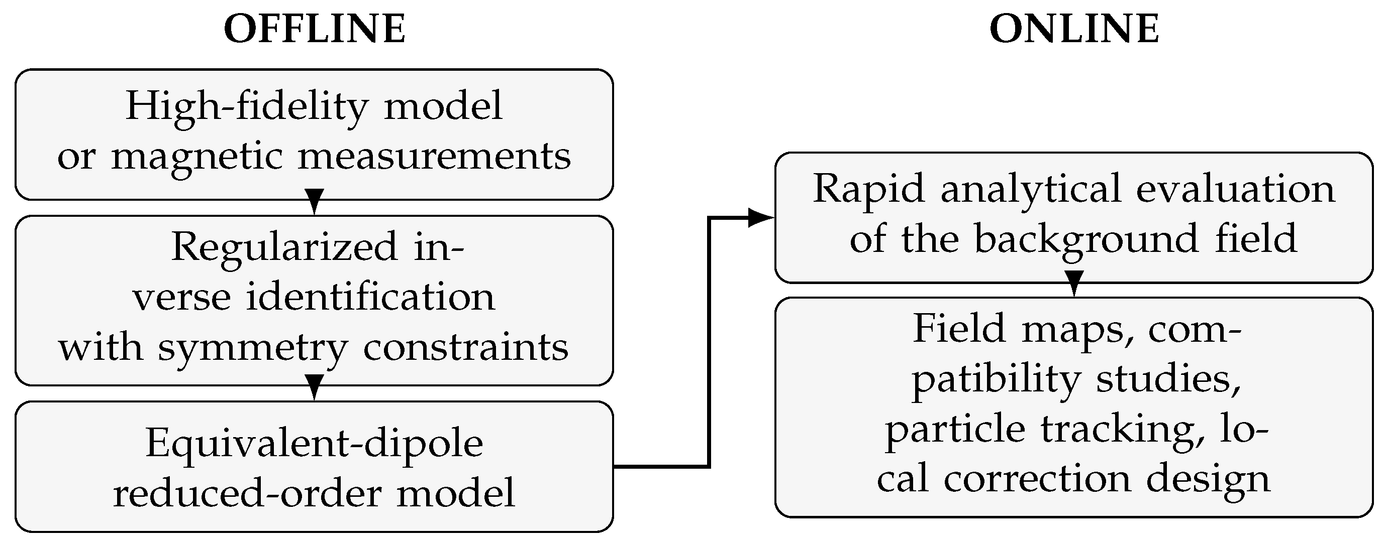
The objective of this work is not to replace the full-order magnetostatic model but to avoid its repeated use whenever the magnetic source remains unchanged. For this reason, the field produced by the original device is represented by a finite set of equivalent magnetic dipoles. Their positions are prescribed, whereas their moments are identified from magnetic-flux-density data obtained from a high-fidelity simulation or, in principle, from measurements. Once this offline calibration has been completed, the external field is evaluated online by direct superposition of closed-form dipole fields. The resulting model is therefore analytical and mesh-free during the evaluation stage.

Figure 1 summarizes the intended use of the method. The full-order model or a set of field measurements is used only in the offline stage to identify the equivalent dipole moments. The calibrated model then provides a reusable background field for repeated evaluations. In a future coupled setting, this background contribution may be superposed with the field computed from a local numerical model, provided that the latter does not significantly alter the magnetic state of the source represented by the equivalent dipoles.

The proposed formulation belongs to the broad family of equivalent-source and auxiliary-source methods. The use of Gauss–Legendre quadrature to replace a distributed magnetic source by an ensemble of equivalent point magnetic dipoles also has a clear precedent in potential-field modeling [23]. However, in the present work, the equivalent sources are not placed on the real geometry of the magnet. Instead, they are located at tensor-product Gauss–Legendre nodes [24,25,26] of a regular auxiliary region, represented by a parallelepiped in the present implementation, which encloses the magnetic assembly. This distinction is essential. The auxiliary domain is not a geometric approximation of the magnet, and the identified dipole moments are not samples of the local magnetization. The parallelepiped provides a deterministic, regular, and symmetry-compatible support for an equivalent-source expansion. Its boundary also defines the natural limit of the intended reconstruction region.

Let ${\mathsf{\Omega }}_{\mathrm{mag}}$ denote the physical magnetic assembly and ${\mathsf{\Omega }}_{\mathrm{aux}}$ the enclosing auxiliary parallelepiped, with ${\mathsf{\Omega }}_{\mathrm{mag}}\subset {\mathsf{\Omega }}_{\mathrm{aux}}$. All equivalent dipoles are contained in ${\mathsf{\Omega }}_{\mathrm{aux}}$, and the reconstructed field is intended for points in

$${\mathsf{\Omega }}_{\mathrm{obs}}\subset {\mathbb{R}}^3\setminus {\overline{\mathsf{\Omega }}}_{\mathrm{aux}}.$$

(1)

Here, the overbar in ${\overline{\mathsf{\Omega }}}_{\mathrm{aux}}$ denotes the topological closure, ensuring that no observation points fall on the domain boundary.

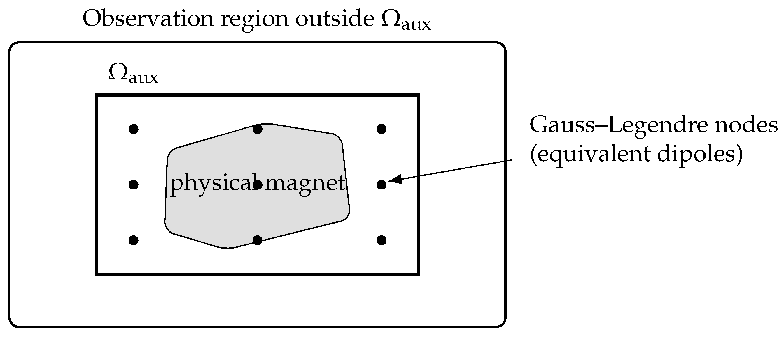
The method should therefore not be described merely as valid “outside the magnet.” Observation points located outside the physical magnet but inside the auxiliary source domain may approach or cross the moving source locations as the quadrature order changes. In that region, convergence can become nonuniform, the identified coefficients can become unstable, and the resulting field should not be interpreted as a reliable approximation of the physical solution. The geometrical relationship among the physical magnet, the auxiliary source domain, the Gauss–Legendre equivalent-source nodes, and the intended observation region is illustrated schematically in Figure 2.

The use of Gauss–Legendre nodes should accordingly be understood as a source- placement strategy rather than as a direct quadrature of the actual magnet geometry. Tensor-product nodes provide a regular family of source configurations of increasing order, preserve reflection symmetries, and provide a convenient non-optimized baseline for source placement. The quadrature weights can be absorbed into the unknown effective moments, which are subsequently identified from field data. This interpretation also avoids attributing a local physical meaning to the equivalent moments.

The reduced-order representation is reusable only while the magnetic source state remains unchanged. In a weakly coupled partition between a source region B and a region of interest A, the total field may be written conceptually as

$${\mathit{B}}_{\mathrm{tot}}\simeq {\mathit{B}}_B^{\mathrm{ROM}}+{\mathit{B}}_A.$$

(2)

Here, ${\mathit{B}}_B^{\mathrm{ROM}}$ is the calibrated background field generated by the fixed source, whereas ${\mathit{B}}_A$ denotes the contribution associated with the region of interest. The decomposition is applicable provided that modifications introduced in A do not significantly perturb the current distribution or magnetic state represented in B. Substantial changes in the source state therefore require recalibration.

The SHiP spectrometer magnet at CERN [6] provides a demanding validation case. Its large dimensions, ferromagnetic yoke, coils, and extended stray-field region lead to a complex full-order model and a costly mesh-generation process. In this work, the reference magnetic field is obtained from a high-fidelity finite-element model, whereas the equivalent dipoles are placed inside a regular auxiliary source domain, represented by a parallelepiped in the present implementation. Model order, calibration-sample distribution, and calibration clearance are then assessed under a controlled protocol before the selected model is subjected to dense post-selection validation.

Within this integrated framework, the specific contributions of the present study can be summarized as follows:

• A unified reduced-order formulation for three-dimensional DC stray fields that combines prescribed equivalent-source placement, symmetry-constrained parameterization, and regularized data-driven identification;
• A clear distinction between the physical magnet, the auxiliary source domain, and the external observation region;
• A family of equivalent-source configurations based on tensor-product Gauss–Legendre nodes of the auxiliary source domain;
• Symmetry-constrained parameterization of the equivalent moments, reducing the number of independent unknowns;
• Regularized inverse identification from magnetic-flux-density data, followed by rapid mesh-free online evaluation;
• A controlled numerical assessment of model order, calibration clearance, and calibration-sample distribution, followed by dense post-selection validation against the high-fidelity SHiP finite-element solution.

The remainder of the paper is organized as follows. Section 2 introduces the equivalent-dipole formulation and the regularized inverse problem. Section 3 describes the auxiliary source domain, the symmetry-constrained source mapping, and the investigated model-order family. Section 4 presents the SHiP case study, the calibration and model-selection protocol, the numerical results, and the dense post-selection validation. Section 5 discusses the accuracy–complexity trade-off, the range of applicability, and possible extensions of the method. Finally, Section 6 summarizes the main findings and conclusions.

2. Mathematical Modeling

Let an ideal magnetic dipole with magnetic moment $\mathit{m}$ be located at ${\mathit{r}}^{\prime }$. For an observation point $\mathit{r}$, define

$$\mathit{R}=\mathit{r}-{\mathit{r}}^{\prime },R=\parallel \mathit{R}\parallel ,\widehat{\mathit{R}}={\displaystyle \frac{\mathit{R}}{R}}.$$

(3)

In free space, considering ${\mu }_0$ as the vacuum magnetic permeability, the magnetic vector potential generated by the dipole is [27,28]

$$\mathit{A}\left(\mathit{r}\right)={\displaystyle \frac{{\mu }_0}{4\pi }}{\displaystyle \frac{\mathit{m}\times \mathit{R}}{R^3}}.$$

(4)

The corresponding magnetic flux density is obtained as

$$\mathit{B}\left(\mathit{r}\right)=\nabla \times \mathit{A}\left(\mathit{r}\right).$$

(5)

Using the identity

$$\nabla \times (\mathit{m}\times \mathit{w})=\mathit{m}\nabla ·\mathit{w}-(\mathit{m}·\nabla )\mathit{w},$$

(6)

with constant $\mathit{m}$, together with

$$\nabla ·{\displaystyle \frac{\mathit{R}}{R^3}}=0,\mathit{R}\ne \mathbf{0},$$

(7)

one obtains

$$\mathit{B}\left(\mathit{r}\right)={\displaystyle \frac{{\mu }_0}{4\pi }}{\displaystyle \frac{3\left(\mathit{m}·\widehat{\mathit{R}}\right)\widehat{\mathit{R}}-\mathit{m}}{R^3}}.$$

(8)

Equation (8) is the exact field of an ideal point dipole for $\mathit{r}\ne {\mathit{r}}^{\prime }$. The approximation involved in the present method does not concern the dipole kernel itself, but rather the replacement of the original magnetic device by a finite set of equivalent dipoles.

For a continuous distribution of dipole moment density $\mathit{M}\left({\mathit{r}}^{\prime }\right)$ occupying a volume $\tau$, the vector potential is

$$\mathit{A}\left(\mathit{r}\right)={\displaystyle \frac{{\mu }_0}{4\pi }}{\int }_{\tau }\mathit{M}\left({\mathit{r}}^{\prime }\right)\times {\displaystyle \frac{\mathit{r}-{\mathit{r}}^{\prime }}{{\parallel \mathit{r}-{\mathit{r}}^{\prime }\parallel }^3}}\mathrm{d}{\tau }^{\prime }.$$

(9)

Taking the curl with respect to the observation coordinates gives

$$\mathit{B}\left(\mathit{r}\right)={\displaystyle \frac{{\mu }_0}{4\pi }}{\int }_{\tau }{\displaystyle \frac{3\left[\mathit{M}\left({\mathit{r}}^{\prime }\right)·\widehat{\mathit{R}}\right]\widehat{\mathit{R}}-\mathit{M}\left({\mathit{r}}^{\prime }\right)}{R^3}}\mathrm{d}{\tau }^{\prime }.$$

(10)

The same continuous magnetization distribution may also be represented by the equivalent volume and surface current densities [28,29]

$${\mathit{J}}_{\mathrm{m}v}={\nabla }^{\prime }\times \mathit{M},{\mathit{J}}_{\mathrm{m}s}=\mathit{M}\times {\mathit{n}}^{\prime },$$

(11)

where ${\mathit{n}}^{\prime }$ is the outward unit normal to the boundary S of $\tau$. Accordingly,

$$\mathit{A}\left(\mathit{r}\right)={\displaystyle \frac{{\mu }_0}{4\pi }}\left[{\int }_{\tau }{\displaystyle \frac{{\mathit{J}}_{\mathrm{m}v}\left({\mathit{r}}^{\prime }\right)}{R}}\mathrm{d}{\tau }^{\prime }+{\int }_S{\displaystyle \frac{{\mathit{J}}_{\mathrm{m}s}\left({\mathit{r}}^{\prime }\right)}{R}}\mathrm{d}{S}^{\prime }\right],$$

(12)

and

$$\mathit{B}\left(\mathit{r}\right)={\displaystyle \frac{{\mu }_0}{4\pi }}\left[{\int }_{\tau }{\mathit{J}}_{\mathrm{m}v}\left({\mathit{r}}^{\prime }\right)\times {\displaystyle \frac{\mathit{R}}{R^3}}\mathrm{d}{\tau }^{\prime }+{\int }_S{\mathit{J}}_{\mathrm{m}s}\left({\mathit{r}}^{\prime }\right)\times {\displaystyle \frac{\mathit{R}}{R^3}}\mathrm{d}{S}^{\prime }\right].$$

(13)

Equation (13) has the form of the Biot–Savart law and shows the equivalence between the magnetization description and the associated bound-current description.

To obtain the finite-dimensional model used in this work, Equation (10) is approximated by a weighted sum over n equivalent dipoles located at the points ${\mathit{r}}_i$:

$$\mathit{B}\left(\mathit{r}\right)\simeq {\displaystyle \frac{{\mu }_0}{4\pi }}{\displaystyle \sum _{i=1}^n}{w}_i{\displaystyle \frac{3\left[{\mathit{m}}_i·{\widehat{\mathit{R}}}_i\right]{\widehat{\mathit{R}}}_i-{\mathit{m}}_i}{R_i^3}},$$

(14)

where

$${\mathit{R}}_i=\mathit{r}-{\mathit{r}}_i,R_i=\parallel {\mathit{R}}_i\parallel ,{\widehat{\mathit{R}}}_i={\displaystyle \frac{{\mathit{R}}_i}{R_i}}.$$

(15)

The coefficients $w_i$ account for the adopted quadrature rule. If the quadrature weights are absorbed into the dipole moments by defining

$${\mathit{p}}_i=w_i{\mathit{m}}_i,$$

(16)

Equation (14) becomes

$$\mathit{B}\left(\mathit{r}\right)\simeq {\displaystyle \frac{{\mu }_0}{4\pi }}{\displaystyle \sum _{i=1}^n}{\displaystyle \frac{3\left[{\mathit{p}}_i·{\widehat{\mathit{R}}}_i\right]{\widehat{\mathit{R}}}_i-{\mathit{p}}_i}{R_i^3}}.$$

(17)

In this representation, ${\mathit{p}}_i$ has units of $\mathrm{A}·{\mathrm{m}}^2$ and represents the effective magnetic moment of the i–th equivalent dipole. Equation (17) is the form used in the direct field reconstruction.

For compactness, define the dipole interaction tensor

$${\mathit{T}}_i\left(\mathit{r}\right)={\displaystyle \frac{1}{R_i^3}}\left(3{\widehat{\mathit{R}}}_i{\widehat{\mathit{R}}}_i^{\mathsf{T}}-\mathit{I}\right).$$

(18)

Then,

$$\mathit{B}\left(\mathit{r}\right)\simeq {\displaystyle \frac{{\mu }_0}{4\pi }}{\displaystyle \sum _{i=1}^n}{\mathit{T}}_i\left(\mathit{r}\right){\mathit{p}}_i.$$

(19)

For P observation points, the three Cartesian field components are stacked in the vector

$$\mathit{b}={\left[\begin{array}{ccccccc}{B}_x\left({\mathit{r}}_1\right)& B_y\left({\mathit{r}}_1\right)& B_z\left({\mathit{r}}_1\right)& \cdots & B_x\left({\mathit{r}}_P\right)& B_y\left({\mathit{r}}_P\right)& B_z\left({\mathit{r}}_P\right)\end{array}\right]}^{\mathsf{T}}\in {\mathbb{R}}^{3P}.$$

(20)

The effective moments of the n equivalent dipoles are collected as

$$\mathit{p}={\left[\begin{array}{cccc}{\mathit{p}}_1^{\mathsf{T}}& {\mathit{p}}_2^{\mathsf{T}}& \cdots & {\mathit{p}}_n^{\mathsf{T}}\end{array}\right]}^{\mathsf{T}}\in {\mathbb{R}}^{3n}.$$

(21)

Let $\mathit{K}\in {\mathbb{R}}^{3P\times 3n}$ denote the matrix assembled from the interaction tensors in Equation (18). The general discrete forward problem can then be written as

$$\mathit{b}={\displaystyle \frac{{\mu }_0}{4\pi }}\mathit{K}\mathit{p}+\mathsf{\epsilon }={\mathit{A}}_0\mathit{p}+\mathsf{\epsilon },$$

(22)

where

$${\mathit{A}}_0={\displaystyle \frac{{\mu }_0}{4\pi }}\mathit{K},$$

(23)

and $\mathsf{\epsilon }$ collects numerical, modeling, and measurement errors.

The least-squares estimate of the effective source moments is

$$\widehat{\mathit{p}}=\arg \underset{\mathit{p}}{\min }{∥{\mathit{A}}_0\mathit{p}-\mathit{b}∥}_2^2.$$

(24)

If

$${\mathit{A}}_0=\mathit{U}\mathsf{\Sigma }{\mathit{V}}^{\mathsf{T}}$$

(25)

is the singular value decomposition of the general interaction matrix, a Truncated Singular Value Decomposition (TSVD) estimate may be written as [30]

$${\widehat{\mathit{p}}}_{\tau }=\sum _{{\sigma }_{\ell }/{\sigma }_1\ge \tau }{\displaystyle \frac{{\mathit{u}}_{\ell }^{\mathsf{T}}\mathit{b}}{{\sigma }_{\ell }}}{\mathit{v}}_{\ell },$$

(26)

where $\tau$ is a relative truncation threshold.

Equation (22) represents the general unconstrained inverse problem. The problem-specific reduction associated with source grouping, reflection symmetries, and symmetry-plane constraints is introduced in Section 3.3, where the complete source vector is parameterized as $\mathit{p}=\mathit{S}\mathit{q}$.

Finally, at distances much larger than the dimensions of the equivalent source distribution, ${\mathit{R}}_i\simeq \mathit{r}$ for every i, and the field reduces to that of the total equivalent magnetic moment

$${\mathit{m}}_{\mathrm{tot}}={\displaystyle \sum _{i=1}^n}{w}_i{\mathit{m}}_i.$$

(27)

Hence,

$$\mathit{B}\left(\mathit{r}\right)\simeq {\displaystyle \frac{{\mu }_0}{4\pi }}{\displaystyle \frac{3\left({\mathit{m}}_{\mathrm{tot}}·\widehat{\mathit{r}}\right)\widehat{\mathit{r}}-{\mathit{m}}_{\mathrm{tot}}}{r^3}},r\gg \underset{i}{\max }\parallel {\mathit{r}}_i\parallel .$$

(28)

This expression provides the asymptotic limit of the multi-dipolar model and confirms the expected $r^{-3}$ decay of the reconstructed stray magnetic field. The adopted source-placement strategy provides a systematic and symmetry-compatible baseline for the equivalent-source representation. The specific tensor-product Gauss–Legendre configurations considered in this work are introduced in Section 3. However, optimization of both the shape of the auxiliary domain and the placement of associated sources remains possible, as discussed in Section 5. In the following section, tensor-product Gauss–Legendre nodes are used for the specific parallelepiped implementation adopted in the present SHiP study. The same equivalent-source concept can be extended to other regular auxiliary domains admitting a convenient quadrature or reference-domain mapping.

3. Symmetry-Constrained Equivalent-Dipole Configurations

The general formulation introduced in Section 2 is now specialized to a finite set of equivalent magnetic dipoles inside an auxiliary domain ${\mathsf{\Omega }}_{\mathrm{aux}}$ that encloses the active magnetic region to be replaced by the reduced-order model. The auxiliary domain is not a geometrical approximation of the real magnet and does not reproduce its material distribution. Its role is instead to provide a regular support for the singular elementary solutions, to permit a deterministic source placement, and to separate the equivalent-source representation from the detailed geometry and finite-element discretization of the original device.

In the implementation considered in this work, ${\mathsf{\Omega }}_{\mathrm{aux}}$ is a parallelepiped centered at ${\mathit{r}}_{\mathrm{c}}$, with half-lengths $h_x$, $h_y$, and $h_z$. The complete physical magnetic assembly is contained inside this auxiliary source region, whereas the field reconstructed from the equivalent dipoles is intended for observation points outside it.

3.1. Gauss–Legendre Source Placement

For a tensor-product Gauss–Legendre rule of orders $(n_x,n_y,n_z)$, the equivalent-source positions are

$${\mathit{r}}_{abc}={\mathit{r}}_{\mathrm{c}}+h_x{\xi }_a^{\left(n_x\right)}\widehat{\mathit{x}}+h_y{\xi }_b^{\left(n_y\right)}\widehat{\mathit{y}}+h_z{\xi }_c^{\left(n_z\right)}\widehat{\mathit{z}},$$

(29)

where

$$a=1,\dots ,n_x,b=1,\dots ,n_y,c=1,\dots ,n_z,$$

(30)

and ${\xi }^{\left(n\right)}$ denotes a one-dimensional Gauss–Legendre node. The total number of physical dipoles is therefore

$$N=n_x{n}_y{n}_z.$$

(31)

As discussed in Section 2, the quadrature weights and the geometric Jacobian may be absorbed into the unknown effective moments. The inverse problem consequently identifies directly the effective magnetic moments ${\mathit{p}}_i$, with units $\mathrm{A}·{\mathrm{m}}^2$. In the present formulation, Gauss–Legendre nodes should therefore be interpreted primarily as a deterministic source-placement strategy rather than as pointwise samples of the real magnetization.

The use of a parallelepiped is a convenient implementation of the method, but it is not a fundamental requirement. More generally, ${\mathsf{\Omega }}_{\mathrm{aux}}$ may be any regular enclosing domain for which a stable Gaussian-type quadrature, or an equivalent mapping from a reference domain, can be constructed conveniently. If $\widehat{\mathsf{\Omega }}$ denotes a regular reference domain, ${\widehat{\mathsf{\xi }}}_i$ its quadrature nodes, and $\mathcal{F}:\widehat{\mathsf{\Omega }}\to {\mathsf{\Omega }}_{\mathrm{aux}}$ a regular mapping, the equivalent-source locations may be written as

$${\mathit{r}}_i=\mathcal{F}\left({\widehat{\mathsf{\xi }}}_i\right).$$

(32)

Accordingly, the shape and dimensions of the auxiliary source region may in principle be treated as design variables and optimized so as to follow more closely the active magnetic region that is to be replaced by the equivalent model. This possibility may reduce unnecessary empty source volume and may improve the representation of the field close to the active region. When symmetry reduction is employed, however, the chosen auxiliary domain and its node distribution must be compatible with the symmetry group of the source region, or the source-group mapping must be modified consistently.

For completeness, the tensor-product family considered in the development of the method is

$$\begin{array}{cc}\hfill (n_x,n_y,n_z)=(2,2,2)& ⟹N=8,\hfill \\ \hfill (n_x,n_y,n_z)=(2,2,3)& ⟹N=12,\hfill \\ \hfill (n_x,n_y,n_z)=(2,3,3)& ⟹N=18,\hfill \\ \hfill (n_x,n_y,n_z)=(3,3,3)& ⟹N=27,\hfill \\ \hfill (n_x,n_y,n_z)=(5,5,5)& ⟹N=125.\hfill \end{array}$$

(33)

Gauss–Legendre rules of different orders are generally non-nested. Equation (33) therefore defines a family of different reduced spaces rather than a conventional nested mesh-refinement sequence. No source order is assumed to be optimal at this stage. The configurations are compared under a common frozen identification protocol in Section 4, where the retained model order is selected from the resulting accuracy–complexity comparison within the prescribed discrete candidate family.

3.2. Reflection Symmetries

The reference SHiP source model exploits the three coordinate planes. With the coordinate convention adopted in this work, its magnetic flux density satisfies

$$\begin{array}{cccc}\hfill \mathit{B}(-x,y,z)& ={\mathit{T}}_x\mathit{B}(x,y,z),\hfill & \hfill {\mathit{T}}_x& =\mathrm{diag}(1,-1,-1),\hfill \end{array}$$

(34a)

$$\begin{array}{cccc}\hfill \mathit{B}(x,-y,z)& ={\mathit{T}}_y\mathit{B}(x,y,z),\hfill & \hfill {\mathit{T}}_y& =\mathrm{diag}(1,-1,1),\hfill \end{array}$$

(34b)

$$\begin{array}{cccc}\hfill \mathit{B}(x,y,-z)& ={\mathit{T}}_z\mathit{B}(x,y,z),\hfill & \hfill {\mathit{T}}_z& =\mathrm{diag}(1,1,-1).\hfill \end{array}$$

(34c)

Equivalent sources located at symmetrically equivalent positions—i.e., sharing the same absolute values of their spatial coordinates—are assigned to the same representative vector group.

Let $g\left(i\right)$ denote the group associated with source i, and let ${\mathit{a}}_g$ denote the representative moment in the non-negative octant. The effective moment of source i is generated as

$${\mathit{p}}_i={\mathit{T}}_x^{{\eta }_{xi}}{\mathit{T}}_y^{{\eta }_{yi}}{\mathit{T}}_z^{{\eta }_{zi}}{\mathit{P}}_{g\left(i\right)}{\mathit{a}}_{g\left(i\right)},$$

(35)

where

$${\eta }_{\alpha i}=\left\{\begin{array}{cc}0,\hfill & r_{i,\alpha }\ge 0,\hfill \\ 1,\hfill & r_{i,\alpha }<0,\hfill \end{array}\right.\alpha \in \{x,y,z\}.$$

(36)

The projector ${\mathit{P}}_g$ eliminates moment components that are incompatible with a source located on a symmetry plane. For the three coordinate planes,

$${\mathit{P}}_x=\mathrm{diag}(1,0,0),{\mathit{P}}_y=\mathrm{diag}(1,0,1),{\mathit{P}}_z=\mathrm{diag}(1,1,0).$$

(37)

This construction embeds the required parity relations directly into the reduced basis. The reconstructed background field therefore satisfies the prescribed reflection properties at arbitrary observation points and not merely at the samples used for calibration.

An important distinction is that the symmetries imposed in Equations (34) are the symmetries of the original source region represented by the reduced model, hereafter denoted as region B. They need not be symmetries of a second region A in which the reconstructed stray field is subsequently used. Thus, region A may contain geometrically asymmetric objects, asymmetric sources, or conductors with a non-symmetric material distribution. In that case, only the background contribution generated by B retains the parities imposed above, whereas the total field in A is not required to be symmetric. This differs from a conventional single-domain finite-element symmetry reduction, for which symmetry boundary conditions can be used to reduce the computational domain only when the complete coupled problem—including geometry, materials, sources, and boundary conditions—is invariant under the same transformation. The present background-field decomposition therefore allows the symmetry of the source region B to be exploited even when the region of interest A does not possess that symmetry.

3.3. Reduced Source Mapping

Let

$$G=⌈{\displaystyle \frac{n_x}{2}}⌉⌈{\displaystyle \frac{n_y}{2}}⌉⌈{\displaystyle \frac{n_z}{2}}⌉$$

(38)

be the number of representative vector groups. The number of independent scalar coefficients is

$$d={\displaystyle \sum _{g=1}^G}\mathrm{rank}\left({\mathit{P}}_g\right).$$

(39)

After stacking the Cartesian components of all physical source moments, the complete moment vector is written as

$$\mathit{p}=\mathit{S}\mathit{q},$$

(40)

where

$$\mathit{p}\in {\mathbb{R}}^{3N},\mathit{q}\in {\mathbb{R}}^d,\mathit{S}\in {\mathbb{R}}^{3N\times d}.$$

(41)

The sparse matrix $\mathit{S}$ contains the group relations, parity transformations, and symmetry-plane constraints.

For P observation points, the reduced forward model is

$$\mathit{b}={\displaystyle \frac{{\mu }_0}{4\pi }}\mathit{K}\mathit{S}\mathit{q}+\mathsf{\epsilon }=\mathit{A}\mathit{q}+\mathsf{\epsilon },$$

(42)

where $\mathit{K}$ collects the closed-form dipole interaction tensors and

$$\mathit{A}={\displaystyle \frac{{\mu }_0}{4\pi }}\mathit{K}\mathit{S}.$$

(43)

For the highest-order candidate in Equation (33),

$$N=125,G=27,d=51.$$

(44)

The distinction among these quantities is important: N is the number of physical point dipoles, G is the number of representative vector groups, and d is the number of independent scalar coefficients. Thus, although the 27 representative vectors nominally contain 81 Cartesian components, the symmetry-plane constraints reduce the number of independent coefficients to 51. Analogous reductions apply to the lower-order configurations.

The source order is selected numerically rather than prescribed a priori. To isolate the effect of model complexity, all configurations in Equation (33) are compared using the same auxiliary domain, calibration data, calibration clearance, frozen spatial split, symmetry constraints, column scaling, and validation-based TSVD procedure. Only the source order and the corresponding reduced dimension are changed. The resulting model-order study is reported in Section 4.3.

4. Numerical Validation for the SHiP Spectrometer Magnet

The proposed reduced-order representation has been assessed using the spectrometer magnet developed for the Scattering and Neutrino Detector of the SHiP experiment at CERN [6]. The reference field is obtained from a three-dimensional COMSOL Multiphysics 6.4 model. The reference finite-element model contains 322,840 elements, with a reported mesh-quality value of $0.92$, and exploits the geometric symmetries of the SHiP magnet. The nonlinear magnetic behavior of the ferromagnetic yoke is represented through its material magnetization curve. The geometry, material properties, and three-dimensional finite-element formulation of the SHiP spectrometer magnet are described in detail in Ref. [6]. The FEM solution is therefore regarded here as the numerical reference rather than as an exact ground truth. Consequently, the errors reported below quantify the discrepancy of the reduced model with respect to this reference solution. The present benchmark considers a single magnetostatic source state. Therefore, all calibration and evaluation data originate from the same underlying finite-element solution, although they are sampled on distinct spatial sets. Accordingly, the reported errors quantify the spatial reconstruction accuracy of the reduced model for this fixed source state and should not be interpreted as evidence of transferability across different excitation or magnetization states.

The numerical study is organized so as to distinguish explicitly between parameter identification, model selection, internal holdout testing, and post-selection assessment. The successive stages comprise the selection of the calibration protocol, the comparison of the equivalent-source order, and the post-selection evaluation of the frozen model on spatial datasets not used in the preceding stages.

4.1. Numerical Protocol and Datasets

For the SHiP application, the auxiliary source domain is the parallelepiped centered at the origin with half-lengths

$$h_x=1.2\mathrm{m},h_y=2.0\mathrm{m},h_z=3.6\mathrm{m}.$$

(45)

For an observation point $\mathit{r}$, its Euclidean distance from this domain is

$$d_{\mathrm{aux}}\left(\mathit{r}\right)={\left[\sum _{\alpha \in \{x,y,z\}}\max {\left(|r_{\alpha }-r_{\mathrm{c},\alpha }|-h_{\alpha },0\right)}^2\right]}^{1/2}.$$

(46)

Two distinct distances are used below. The calibration clearance $d_{\mathrm{cal}}$ is the minimum $d_{\mathrm{aux}}$ admitted during inverse identification, whereas $d_{\mathrm{valid}}$ is a post-calibration empirical boundary defining the external region in which the selected model meets the adopted accuracy criterion.

Two first-octant calibration grids with the same nominal size (35 × 35 × 11 = 13,475 nodes) were compared. The exponential grid contains a higher density of points near the magnetic source, while the uniform grid is evenly spaced. Both grids span $0\le x,y\le L_{xy}$, with $L_{xy}=7.379\mathrm{m}$, and contain 35 coordinates along each of these directions. For $j=0,\dots ,34$, the uniform grid uses $x_j=y_j=j{L}_{xy}/34$, whereas the exponential grid uses $x_j=y_j=L_0[\exp \left\{(j/34)\ln (1+L_{xy}/L_0)\right\}-1]$, with $L_0=1\mathrm{m}$. Both grids use the same 11 coordinates along z, namely $z_k=0.001+0.720k\mathrm{m}$, with $k=0,\dots ,10$. After removing non-finite and non-external samples, they provide 9750 and 8111 external observations, respectively. A third shifted regular grid, containing 17,104 finite external points over $0.325\le d_{\mathrm{aux}}\le 5.0$ m, is used only as a common sensitivity/model-selection grid. Because this grid was used to compare calibration clearances and source orders, it is treated explicitly as a sensitivity/model-selection dataset and is not regarded as an independent final validation set. All reported calibration and common-grid errors are computed from the finite strictly external first-octant samples. Reflection to the other octants leaves the relative vector $L^2$ error unchanged because both fields satisfy the same verified parities.

For each calibration grid, all finite observations strictly external to the auxiliary domain were partitioned through a deterministic, balanced blockwise spatial train/validation/test split. The occupied coordinate ranges were divided into five, five, and four intervals along the three Cartesian directions, respectively, defining up to $5\times 5\times 4=100$ rectangular blocks. In the present datasets, 83 of these blocks are occupied. Each occupied block was assigned in its entirety to one subset, thereby preventing spatial leakage between training, validation, and testing.

The assignment targeted nominal point fractions of $60\%$, $20\%$, and $20\%$ and was optimized to balance the total number of observations, the distribution of $d_{\mathrm{aux}}$, the distribution of the reference-field magnitude, and their joint distribution. A fixed random seed $260,805$ was used for 6000 multistart assignments, followed by up to 12 local-improvement passes based on single-block moves and pairwise block swaps.

The block assignment was generated once using all finite strictly external calibration points and was then kept frozen throughout the clearance and model-order studies. For each value of $d_{\mathrm{cal}}$, points not satisfying $d_{\mathrm{aux}}\ge d_{\mathrm{cal}}$ were removed from their preassigned subsets without any reassignment. 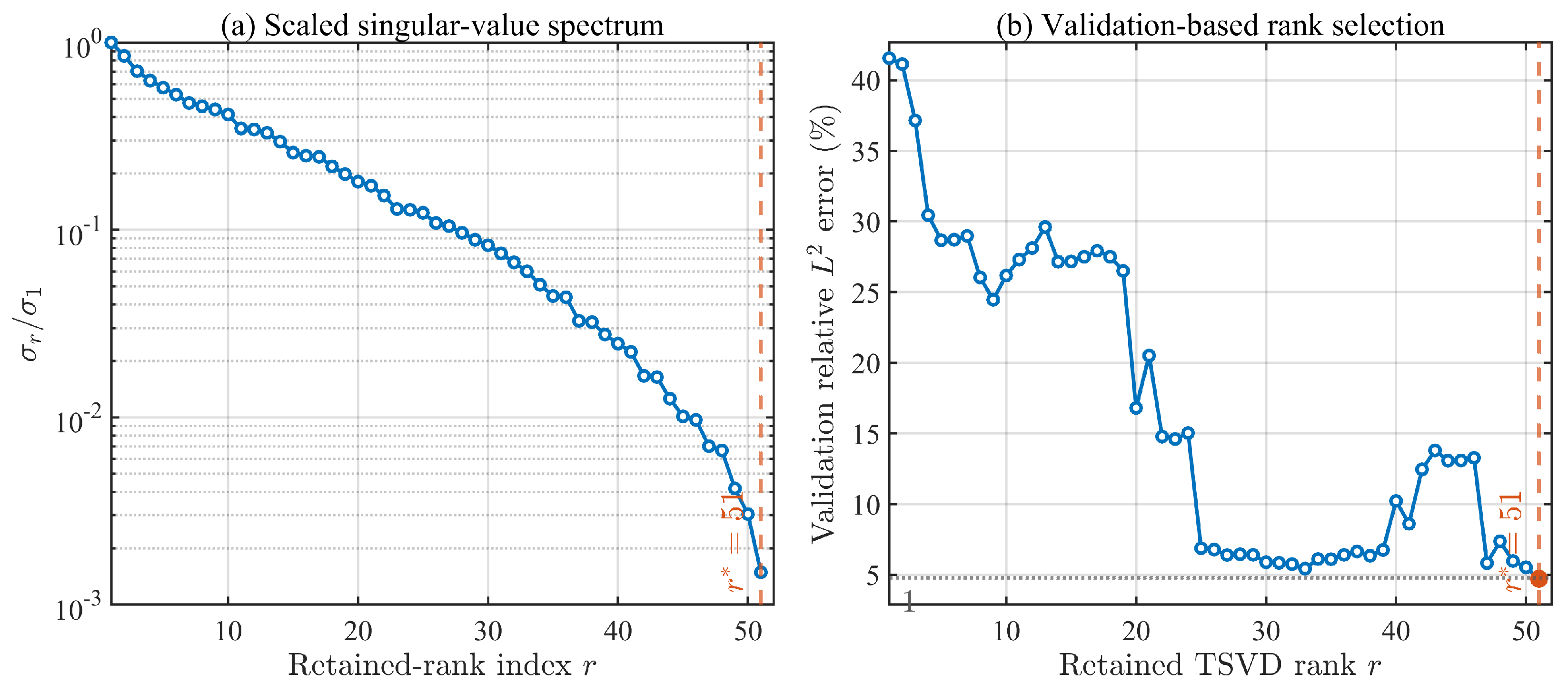The design matrix was column-scaled before TSVD, and the selected rank was the smallest rank whose validation error lay within $1\%$ of the minimum validation error. After rank selection, the coefficients were re-estimated using the union of the training and validation subsets. The test subset was not used either for coefficient fitting or for TSVD-rank selection and therefore constitutes a spatially blockwise holdout. For the selected exponential-grid configuration at $d_{\mathrm{cal}}=0.40$ m and $N=125$, Figure 3 shows the normalized singular values of the column-scaled training matrix and the corresponding validation error as a function of the retained TSVD rank. The prescribed $1\%$ validation rule selects $r=51$.

For the subsequent model-order comparison, the exact frozen train/validation/test indices associated with the selected exponential calibration case at $d_{\mathrm{cal}}=0.40$ m were reused for every investigated source order. Consequently, differences among the model-order results cannot originate from changes in the observations assigned to the identification subsets. The resulting test subset therefore constitutes a spatially blockwise holdout, since entire spatial blocks are excluded from both coefficient fitting and TSVD-rank selection.

The principal global accuracy measure is the relative vector error

$$e_{\mathrm{rel},2}={\displaystyle \frac{{∥{\mathit{B}}_{\mathrm{EDM}}-{\mathit{B}}_{\mathrm{FEM}}∥}_{\mathrm{F}}}{{∥{\mathit{B}}_{\mathrm{FEM}}∥}_{\mathrm{F}}}}.$$

(47)

where ${\mathit{B}}_{\mathrm{EDM}}$ and ${\mathit{B}}_{\mathrm{FEM}}$ denote the fields reconstructed by the equivalent-dipole model (EDM) and computed by the reference finite-element model (FEM), respectively. Furthermore, the subscript “F” denotes the Frobenius norm, which computes the square root of the sum of the absolute squares of its elements, whereas the subscript “2” denotes the standard Euclidean norm (or $L^2$ norm) in ${\mathbb{R}}^3$, applied to the local magnetic flux density vector evaluated at a specific spatial point $\mathbf{r}$. Here, ${\mathit{B}}_{\mathrm{EDM}},{\mathit{B}}_{\mathrm{FEM}}\in {\mathbb{R}}^{P\times 3}$ are point-by-component field matrices. Their Frobenius norm is equivalent to the Euclidean norm of the corresponding stacked field vector defined in Equation (20).

For the error maps, the pointwise relative vector error is

$${\epsilon }_{\mathrm{rel}}\left(\mathit{r}\right)=100{\displaystyle \frac{{∥{\mathit{B}}_{\mathrm{EDM}}\left(\mathit{r}\right)-{\mathit{B}}_{\mathrm{FEM}}\left(\mathit{r}\right)∥}_2}{{∥{\mathit{B}}_{\mathrm{FEM}}\left(\mathit{r}\right)∥}_2}}.$$

(48)

Equation (48) is evaluated only where $\parallel {\mathit{B}}_{\mathrm{FEM}}{\left(\mathit{r}\right)\parallel }_2>0$. Since this pointwise normalization may amplify the apparent error where the reference field is very small, the global vector norm $e_{\mathrm{rel},2}$ remains the primary quantitative metric. Distance-resolved errors are also evaluated in $0.05$-m shells. The quantity $d_{5\%}$ denotes the lower boundary of the first shell containing at least 50 finite external points for which the shell relative vector error is below $5\%$ and remains below $5\%$ for all subsequent shells. The $5\%$ threshold is adopted here as a pragmatic accuracy criterion for defining the empirical validity boundary and should not be interpreted as a regulatory or safety limit.

4.2. Calibration Clearance and Sampling Strategy

Table 1. Representative calibration-clearance results for the 125-dipole model. Errors are evaluated on the common three-dimensional sensitivity/model-selection grid.

	Exponential Calibration Grid			Uniform Calibration Grid
${\mathit{d}}_{\mathrm{cal}}$ [m]	${\mathit{r}}_{\mathrm{TSVD}}$	${\mathit{e}}_{\mathrm{rel},\mathbf{2}}$ [%]	${\mathit{d}}_{\mathbf{5}\%}$[m]	${\mathit{r}}_{\mathrm{TSVD}}$	${\mathit{e}}_{\mathrm{rel},\mathbf{2}}$[%]	${\mathit{d}}_{\mathbf{5}\%}$[m]
0.00	1	61.4	–	4	49.5	–
0.20	51	5.09	0.55	50	5.95	0.55
0.40	51	4.59	0.45	50	5.61	0.50
0.60	49	6.88	0.55	48	6.32	0.55
1.00	50	8.90	0.55	50	11.0	0.60

reports representative results of the clearance sweep for the 125-dipole candidate. The parameter $r_{\mathrm{TSVD}}$ denotes the truncation rank, i.e., the number of retained singular values. Using all external points ($d_{\mathrm{cal}}=0$) strongly destabilizes the identification: validation retains only one singular direction for the exponential grid and four for the uniform grid, with common-grid errors of $61.447\%$ and $49.544\%$, respectively. Increasing the clearance first improves stability and predictive accuracy, whereas excessive clearance removes the near-source information required to reconstruct the near/intermediate field.

The best overall compromise for the exponential calibration is

$$d_{\mathrm{cal}}=0.40\mathrm{m},$$

(49)

for which all 51 singular directions are retained and the scaled condition number is $6.71\times {10}^2$. At the same clearance, the exponential grid gives a lower global common-grid error than the uniform grid ($4.59\%$ versus $5.61\%$) and improves the near/intermediate-field shells. Farther from the source, the two strategies become very similar, with the uniform grid slightly better in some far-field metrics. The result is therefore interpreted as a sampling-distribution effect, not as a universal superiority of the exponential grid. For the selected exponential-grid calibration at $d_{\mathrm{cal}}=0.40$ m, the frozen blockwise partition retains 5567, 1762, and 1677 observations in the training, validation, and test subsets, respectively. The test subset, which is not used for either coefficient identification or TSVD-rank selection, yields a relative vector error of $e_{\mathrm{rel},2}=4.20\%$.

Sensitivity to imperfect calibration data was assessed by adding independent Gaussian perturbations with prescribed relative $L^2$ amplitudes of $0.1\%$, $0.5\%$, $1\%$, $2\%$, and $5\%$ to the training and validation field values. For each nonzero noise level, 50 realizations were considered, while the source configuration, calibration clearance, spatial split, column scaling, and TSVD selection rule were kept unchanged. Up to $2\%$ noise, the selected rank remained $r=51$ in every realization and the median error on the unperturbed blockwise test subset remained between $4.19\%$ and $4.20\%$; at $2\%$ noise, its 5th–95th percentile interval was $4.10$–$4.32\%$. At $5\%$ noise, the median test error was $4.26\%$, although 9 of the 50 realizations selected $r=33$, increasing the 95th-percentile test error to $9.87\%$.

4.3. Model-Order Selection

After fixing the calibration protocol above, the five source configurations of Section 3 were compared while keeping the auxiliary domain, exponential calibration grid, $d_{\mathrm{cal}}=0.40$ m, frozen spatial split, column scaling, symmetry constraints, and TSVD selection rule unchanged. Thus only the reduced-model order is varied, as summarized in

Table 2. Model-order sensitivity under the frozen identification protocol. A dash indicates that the persistent $5\%$ shell criterion is not reached within the investigated external domain.

$({\mathit{n}}_{\mathit{x}},{\mathit{n}}_{\mathit{y}},{\mathit{n}}_{\mathit{z}})$	N	G	d	${\mathit{r}}_{\mathbf{TSVD}}$	${\mathit{\kappa }}_2\left(\overline{\mathit{A}}\right)$	${\mathit{e}}_{\mathbf{rel},2}$ [%]	${\mathit{d}}_{5\%}$ [m]
$(2,2,2)$	8	1	3	1	1.10	85.3	–
$(2,2,3)$	12	2	5	3	1.83	66.9	–
$(2,3,3)$	18	4	8	5	3.81	55.0	–
$(3,3,3)$	27	8	12	11	8.24	21.2	2.00
$(5,5,5)$	125	27	51	51	671	4.59	0.45

.

The transition from $N=27$ to $N=125$ is decisive: the global common-grid error decreases from $21.2\%$ to $4.59\%$, while $d_{5\%}$ decreases from $2.00$ m to $0.45$ m. For $d_{\mathrm{aux}}\ge 0.50$ m, the cumulative relative vector error falls from $13.7\%$ to $1.71\%$. Although the highest-order system is more ill-conditioned, the validation rule selects $r=51$ for the present unperturbed calibration dataset, so that no singular direction is truncated in this particular fit.

Within the investigated discrete candidate family, these results justify retaining

$$N=125$$

(50)

as the best-performing tested configuration. This selection should not be interpreted as establishing a global accuracy–complexity optimum; a denser assessment of intermediate and higher tensor-product orders would be required for that purpose.

4.4. Final Validity Domain and Post-Selection Validation

For the selected exponential 125-dipole model, the common-grid shell analysis gives $d_{5\%}=0.45$ m. A conservative operational value

$$d_{\mathrm{valid}}=0.50\mathrm{m}$$

(51)

is adopted. The imposed reflection parities are satisfied to floating-point accuracy, with relative defects of order ${10}^{-16}$.

After the calibration distribution, calibration clearance, source order, regularization procedure, and validity boundary had been fixed, an additional dense uniform three-dimensional COMSOL dataset was generated exclusively for post-selection assessment. The grid has a spacing of $0.10$ m and contains 232,560 nominal points; among these, 177,743 finite external observations satisfy $d_{\mathrm{aux}}\ge 0.50$ m. No coefficient fitting or model-selection decision was performed using these data. On this three-dimensional post-selection dataset, the frozen $N=125$ model gives a relative vector $L^2$ error of $1.77\%$, a vector MAE of $5.52\mathsf{\mu }\mathrm{T}$, and a 95th-percentile absolute vector error of $21.4\mathsf{\mu }\mathrm{T}$.

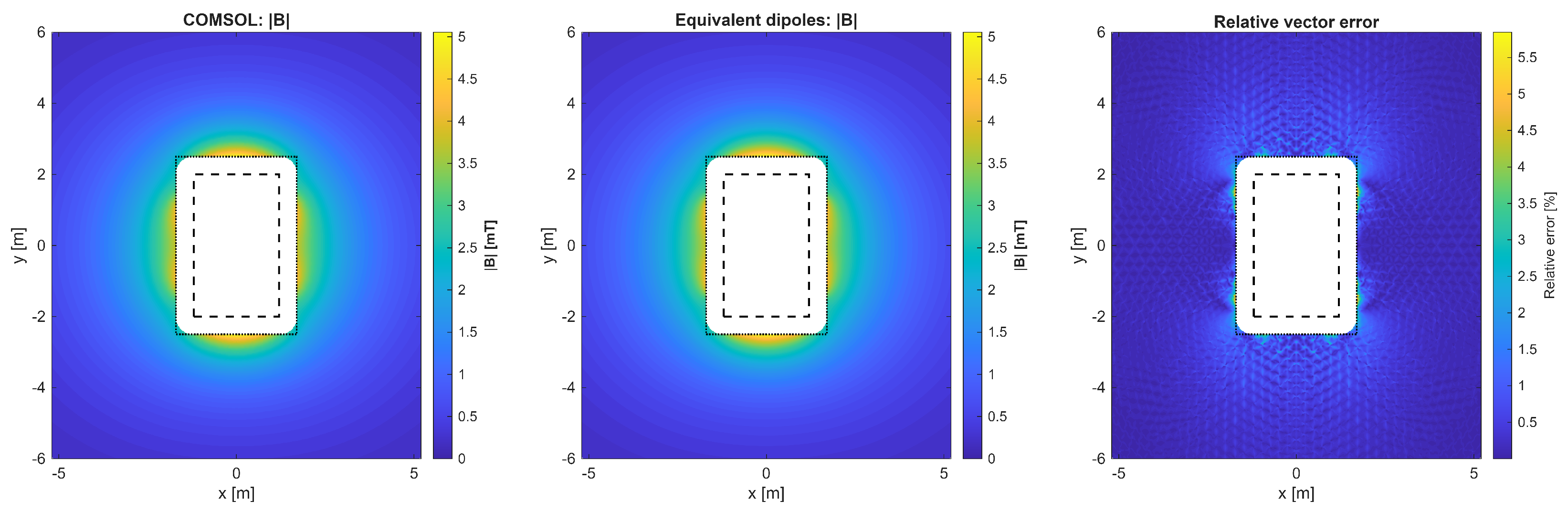
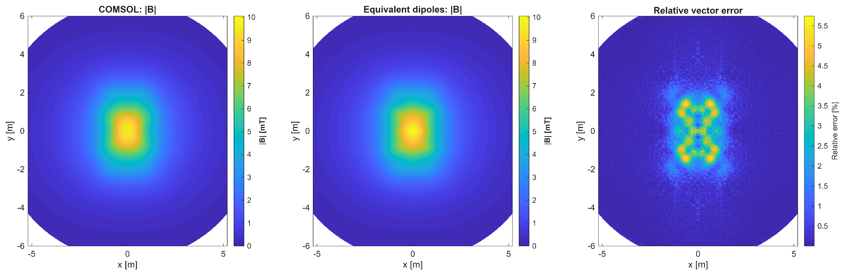
The two dense COMSOL planes reported below were likewise generated after the model-development choices had been frozen and are retained as complementary spatially resolved assessments of the same reduced model. On the physically representative mid-plane $z=0$, the 43,635 finite points satisfying $d_{\mathrm{aux}}\ge 0.50$ m give

$$e_{\mathrm{rel},2}=0.95\%.$$

(52)

The vector MAE and 95th-percentile absolute vector error are $5.40\mathsf{\mu }\mathrm{T}$ and $21.6\mathsf{\mu }\mathrm{T}$, respectively. The distance-resolved result independently confirms the adopted validity boundary: the shell $0.40\le d_{\mathrm{aux}}<0.50$ m gives $5.01\%$, whereas the next shell, $0.50\le d_{\mathrm{aux}}<0.60$ m, gives $2.09\%$ and the error continues to decrease with distance. The corresponding field and error maps are shown in Figure 4.

A second dense plane at $z=4.125$ m, shown in Figure 5, is entirely outside the conservative validity boundary and provides a complementary check over 47,879 finite external points, for which

$$e_{\mathrm{rel},2}=2.74\%.$$

(53)

Unlike the mid-plane, this plane does not intersect the auxiliary source region because its minimum clearance is $0.525$ m. It therefore provides a complementary fully external validation of the same frozen model.

4.5. Computational Cost and Online Evaluation

The computational cost of the proposed approach was assessed by separating the one-time offline stage from the subsequent online field-evaluation stage. All timings were obtained on the same computational platform, i.e., a workstation equipped with an 11th Gen Intel^® Core^TM i7-1165G7 @2.80 GHz and NVIDIA GeForce MX450, using COMSOL Multiphysics^® 6.4 and MATLAB^® R2025b. Unless otherwise stated, figure rendering and file-writing operations were excluded from the timing measurements.

The full-order finite-element solution required 1936 s. Evaluation and export of the field data used for calibration required an additional time of about 2 s. Once the reference data were available, assembly of the reduced inverse problem for the selected $N=125$ configuration required $1.30$ s, while column scaling, singular-value decomposition, validation-based rank selection, and final refitting required $0.061$ s. The EDM-specific offline identification therefore required $1.36$ s, whereas the complete one-time offline workflow, including generation and extraction of the finite-element reference data, required approximately 1939 s, as summarized in

Table 3. Computational cost of the full-order finite-element model and the selected equivalent-dipole model.

Operation	Wall Time
FEM stationary solution	1936 s
FEM calibration-data evaluation/export	≈2 s
EDM matrix assembly	$1.30$ s
EDM scaling, SVD, rank selection, and final fit	$0.061$ s
Dense 3-D EDM evaluation (177,743 points)	$0.65$ s
Dense 3-D FEM evaluation/export (177,743 points)	≈2 s

.

For the dense three-dimensional set of 177,743 observation points, online evaluation of the calibrated equivalent-dipole model required $0.65$ s, whereas evaluation and export at the same points from the already computed full-order finite-element solution required about 2 s. The corresponding online speed-up was therefore approximately $3.10$.

These results clarify the computational role of the proposed model. In the present FEM-calibrated implementation, the equivalent-dipole approach does not eliminate the one-time computational cost required to establish the reference magnetic state. Rather, this cost is incurred during the offline stage and is subsequently amortized over repeated field evaluations. Once calibrated, the magnetic state is represented by a compact set of equivalent-dipole coefficients, so that subsequent evaluations do not require re-solving the full-order problem or retaining and interrogating its complete discretized representation.

5. Discussion

The results confirm that the proposed model is a data-calibrated reduced-order representation of the external field of a source whose magnetic state is known during the offline stage. The equivalent dipoles are not a discretization of the real magnetization; rather, they provide a compact analytical basis for reproducing the field outside the auxiliary source support.

5.1. Identification Strategy and Model Complexity

The numerical study shows that calibration clearance, sampling distribution, and model order are coupled design choices. Including points arbitrarily close to ${\mathsf{\Omega }}_{\mathrm{aux}}$ does not improve the reduced model: the rapidly varying near-boundary field and the singular elementary basis make the inverse problem more difficult, and validation then suppresses most singular directions. Conversely, excessively large clearances remove observations that constrain the near/intermediate field. The selected value $d_{\mathrm{cal}}=0.40$ m represents the best compromise for the present configuration, whereas $d_{\mathrm{valid}}=0.50$ m is an independent empirical statement about the predictive domain.

The calibration-grid comparison likewise shows that sampling should be designed for the region of interest. The exponential grid improves the near/intermediate-field reconstruction, while the uniform grid becomes slightly more accurate in some far-field metrics; therefore, no universal superiority of one distribution is claimed.

Finally, the number of dipoles is properly interpreted as a reduced-model order, not as a finite-element mesh density. The $N=125$ model is retained because the improvement over $N=27$ is substantial: the common-grid error decreases from $21.2\%$ to $4.59\%$ and $d_{5\%}$ from $2.00$ m to $0.45$ m. Although the scaled condition number increases, the validation rule selects $r=51$ for the present dataset. The richer source space is therefore required to represent spatial content that is not captured by the lower-order models, particularly close to the intended validity boundary.

5.2. Generality of the Equivalent-Source Formulation

This section summarizes the broader applicability of the proposed formulation, generalizing the conceptual points introduced earlier in the manuscript beyond the specific case study.

While the parallelepiped geometry used in the SHiP study is highly convenient—as it supports a straightforward tensor-product Gauss–Legendre construction and facilitates reflection-group mappings—it is merely one possible implementation. As noted previously, this bounding box must not be identified with the physical geometry of the magnet. The theoretical framework can be extended to any suitable auxiliary enclosing solid that admits a robust quadrature rule or a convenient mapping from a reference domain. Therefore, its shape and dimensions may in principle be treated as design variables and optimized to follow the active source region more closely. Such an optimization should balance enclosure of the physical sources, conditioning, distance from the intended observation region, and compatibility between the node distribution and the symmetry group used in the reduced mapping.

The imposed symmetry constraints belong to the source region B represented by the reduced model and need not be shared by the local region A. Hence, asymmetric geometry, materials, conductors, or local sources may be treated in A while retaining the symmetry-reduced background field generated by B. This differs from a monolithic FEM symmetry reduction, which requires the complete coupled problem to be invariant under the same transformation.

With reference to the weakly coupled decomposition introduced in Equation (2), the present DC model provides the background contribution generated by region B, provided that the reaction field associated with region A does not appreciably alter the source state used for calibration.

5.3. Limitations and Outlook

The present coefficients are calibrated from a high-fidelity finite-element solution. Identification from measurements is possible in principle, but sensor uncertainty, positioning errors, incomplete coverage, and systematic offsets would then need explicit treatment. Moreover, the reported $d_{\mathrm{valid}}$ is configuration-dependent: changes in the auxiliary support, source order, operating state, sampling distribution, or regularization require renewed distance-resolved verification.

Gauss–Legendre placement also does not by itself regularize the inverse problem. Instead, column scaling and TSVD remain important. Future developments may therefore address optimized auxiliary domains, adaptive or multiple source layers, mixed dipole–multipole bases, measurement-based calibration, uncertainty propagation, and parametric or time-dependent coefficient models.

A possible extension of the present formulation concerns weakly coupled magnetoquasistatic problems with a time-varying background field. In this case, the full-order model may be solved at a sequence of selected time instants, and the corresponding reduced coefficients may be identified from the total magnetic field at each sampled state. The equivalent-source representation does not require the individual contributions to the total field to be separated; therefore, imposed currents, ferromagnetic magnetization, and eddy-current contributions within source region B can all be implicitly incorporated into the time-dependent coefficient vector $\mathit{q}\left(t\right)$. The resulting coefficient snapshots may then be interpolated to provide the background excitation for a local time-dependent problem in region A. The temporal sampling must, however, be sufficiently fine to resolve the fastest field variations relevant to the intended application. In particular, transient field peaks associated with strong induced currents must be adequately sampled to avoid their loss during interpolation. As in the static formulation, this weakly coupled use requires the electromagnetic back-reaction of region A on the source state represented in region B to remain negligible. This time-dependent extension is not validated in the present work and is therefore left for future investigation.

6. Conclusions

A symmetry-constrained equivalent-dipole reduced-order model has been developed for the rapid reconstruction of three-dimensional DC stray magnetic fields. The method represents the external field of a fixed magnetic source through a finite superposition of closed-form point-dipole fields whose effective moments are identified by a one-time regularized inverse problem.

For the SHiP spectrometer case study, five symmetry-constrained model orders were compared under the same identification protocol. The final configuration contains $N=125$ physical dipoles arranged into $G=27$ representative vector groups and requires $d=51$ independent scalar coefficients. Compared with the $N=27$ configuration, the common three-dimensional evaluation-grid error decreases from $21.2\%$ to $4.59\%$, providing a quantitative justification for the selected model order.

After the calibration distribution, clearance, regularization, model order, and validity boundary had been fixed, an additional dense three-dimensional COMSOL dataset was generated exclusively for post-selection assessment. Over approximately $1.78\times {10}^5$ finite external points satisfying $d_{\mathrm{aux}}\ge 0.50$ m, the selected model gives a relative vector $L^2$ error of $1.77\%$, with a vector MAE of $5.52\mathsf{\mu }\mathrm{T}$ and a 95th-percentile absolute vector error of $21.4\mathsf{\mu }\mathrm{T}$. The complementary dense mid-plane assessment gives a relative vector $L^2$ error of $0.95\%$ over $4.4\times {10}^4$ points in the same validity region. Together with the distance-resolved analysis, these results support the conservative empirical validity distance $d_{\mathrm{valid}}=0.50$ m adopted for the final model.

The proposed representation complements rather than replaces the full-order magnetostatic analysis. Once the magnetic state of the source has been established, the calibrated model provides a compact analytical representation for mesh-free online evaluation of the external field provided that the source state remains unchanged. By contrast, substantial changes in geometry, excitation, or magnetization generally require a new calibration.