A 2-Dimensional Continuous Wavelet Transform Technique for Composite Panel Inspections by Scanning Laser Doppler Vibrometry

Abstract

Lamb waves propagation analysis is among the leading-edge approaches for the Non-Destructive Testing of composite thin-walled structures. The underlying diagnostic principle relies on the dependence of elastic waves wavelength on the plate thickness through which they propagate. Therefore, critical defects in composite panels, such as delaminations, can be detected by a non-contact, automated and high-resolution method such as Laser Doppler Vibrometry. The general approach applied in signal processing is referred to as Local Wavenumber Estimation. It consists of creating an image of the average wavelength over the acquisition frequency band in which the pixel element corresponds to a point of the vibrometer scan grid. The standard signal processing approach is typically implemented via the Short Space Fourier Transform. While effective at creating an average wavelength image over the acquisition frequency band, a major drawback of the Short Space Fourier Transform is its heavy reliance on the a priori selection of a spatial window size; a suboptimal choice can severely degrade detection robustness and spatial resolution. To overcome this limitation, we propose a novel method based on the 2D Continuous Wavelet Transform for the detection of defects in composite structures based on the isotropic Morlet wavelet. Thereafter, the proposed method is experimentally validated exploiting a glass fiber reinforced plate with an induced delamination. The proposed method proves superior on average by eliminating parameter dependency while preserving the original image resolution, resulting in a 66% Intersection over Union metric, comparable with the values of the standard method, but with a lower computational time.

1. Introduction

The advent of composite materials has allowed for the enhancement of structural performances, providing high strength, low weight, high-fatigue and corrosion resistance [1]. Consequently, the need for efficient, non-destructive and reliable inspection methods for defect or damage detection has emerged as a direct consequence of such an advent. A variety of tailored NDT techniques have been developed depending on the specific composite configuration. For instance, Shearography inspection has been proposed to improve defect estimation [2]; electromagnetic wave NDT approaches have been successfully applied to assess carbon fiber-reinforced polymers [3]. Ultrasonic techniques remain prominently utilized, exploiting both advanced methods for weak bond detection in composite-adhesive joints [4] and air-coupled magnetostrictive transducers for broader composite evaluations [5]. Furthermore, infrared vision has proven effective in revealing subsurface defects in impact-loaded Kevlar structures [6] and in thick-walled composites [7]. In this scenario, wave propagation is extensively exploited in the context of damage detection, classification and quantification. Specifically, ultrasonics guided waves are widely investigated in the literature in terms of numerical analysis, for example, using FEM, and consequently exploited for experimental inspections. In the domain of numerical modeling, Ge et al. [8] developed a novel spectral FEM for the accurate simulation of PZT-induced Lamb waves propagation, while Guers and Tittmann [9] focused on the simulation of ultrasonics waves in rectangular bar specimens for monitoring nuclear environment. Furthermore, these numerical and theoretical foundations have been extensively exploited for targeted experimental defect characterization across various materials. For instance, experimental inspections exploiting Lamb waves have been successfully utilized to assess the integrity of disbonded honeycomb composite structures [10]. In the context of more complex multi-layered and composite materials, researchers have applied these guided waves to estimate disbond contours in aluminum/CFRP adhesive joints based on phase velocity variations [11], as well as to investigate wave interactions with delamination edges in CFRP composites, thereby enabling advanced reference-free localization methods. Lamb waves are defined as guided waves able to pass through long paths inside thin plates. They are by definition dispersive, i.e., their velocity depends on frequency, and their propagation is influenced by angle, excitation, material characteristics and geometry [12]. Lamb waves can be classified into two types of modes, symmetric modes and anti-symmetric modes. The characteristics of these were reported in [13], where the authors numerically demonstrated that a change in propagation velocity occurs when a delamination is present. More precisely, mode conversions have been identified in correspondence of defect boundaries for both S0 and A0 waves. This method is applicable in plate-like structures and validated for rather big defect dimensions (5–25 cm). This results in a limitation but, on the other side, the proposed conditions enabled a clear sensitivity study about the influence of defect orientation and width, and the influence of the configuration of sensing and excitation points. In particular, the results of the numerical analysis showed that the defect orientation can be determined by using at least three unaligned sensors, while for what concerns damage size evaluation, an accurately designed distribution of sensors is required. The more strewn the sensors are, the longer the damage can be identified. In [10], the authors confirmed that the A0 mode is very effective for delaminations and debonding detection also in layered and sandwich plates, resulting in an increase in signal amplitude according to the defect, and in a lower velocity of propagation, i.e., in a deformation of the wavefront according to the frequency times the thickness product. As can be deduced from the previous lines, numerical analysis and simulations play a very important role in the characterization of wave propagation phenomenon and in providing useful indications for experimental setup. However, for multiple reasons they cannot substitute experimental measurements and analysis, thus the need of developing robust and reliable inspection methods for damage detection by exploiting Lamb Waves. A primary reason for this necessity is that real-world inspections must account for complex operational variables often idealized in simulations, such as surface conditions. In composite materials, tribological characteristics and wear are crucial but challenging. Surface roughness significantly affects Lamb wave propagation, inducing dispersion scattering and amplitude attenuation. Based on studies such as [14], surface roughness-related structural attenuation can be substantial (e.g., 1 to 100 Np/m), differently affecting the various Lamb wave propagation modes.

Lamb waves propagation has been largely analyzed in the literature by means of Wavelet Transforms. The use of wavelets allows to select appropriate scales in order to filter out the effects of macroscopic vibration in the structure under test. Zima et al. [15] exploited the CWT to achieve the wavefront shape reconstruction by precisely extracting time-of-arrival data from Lamb wave signals, even with limited sensors. This Wavelet-processed data proved to enable the accurate reconstruction of the wavefront, allowing for defect localization based on geometric distortions. In [16], an MDI algorithm for inspecting delamination defects in carbon fiber composite plates was discussed. In particular, Lamb waves were emitted and received by air-coupled ultrasonic transducers. Compared with the XY direction-step scanning method used in the traditional delamination defect detection, the authors adopted the 360° rotation scanning method to store the omni-directional information of the inspected area. The proposed algorithm consists of three steps: Wavelet threshold denoising (selection of an appropriate threshold after applying the Wavelet Transform to the signal), EMD and Hilbert transform. In order to characterize the delamination, time-domain amplitude and the instantaneous energy obtained by Multimodal Decomposition were exploited. In conjunction with MDI, cross-correlation coefficients between the damaged and undamaged signals were retrieved in order to determine a damage index, thus the need of a defect-free signal. In [17], multiple baseline signals from the undamaged one-dimensional structure were required as well, and the Lamb wave propagation were induced by PZT. Moreover, the work presented a decision-making approach, involving signal processing and statistical analysis, using AHWT and PCA applied to the Wavelet coefficients, to show the critical features of Lamb wave propagation in the undamaged structure. The detection of damage was obtained by a feature comparison between signal collected from the test structure and baseline signals. Similarly, in [18] Lamb Wave propagation through aerospace composites has been investigated by the use of Wavelet technique to detect an impact damage. The analysis was conducted before and after the impact. As a result, variations in the Lamb waves interacting with the damaged structure were computed by this Wavelet approach, by evaluating the amplitude change of the Wavelet coefficients. In [19], a quantitative relation between anisotropic wavefront and propagation direction was defined to highlight the direction dependency of Lamb wave propagation in composite laminates, involving also damaged ones, determining in the end the ToF of the Lamb Waves. The method was experimentally tested on a cross-ply laminate excited by PZT transducers, a scanning LDV was used to collect the out-of-plane displacement of the testing points, and a Gabor wavelet based CWT was exploited for a better estimation of the ToF, resulting in a satisfying damage localization. Moreover, in [18] the authors proposed a system to detect and localize delaminations in Kevlar/epoxy specimens by exploiting Lamb waves produced by a piezoelectric transducer and received by an accelerometer. The A0 mode was chosen in this work as diagnostic wave, since it has been found to be strongly reflected by delaminations. In order to evaluate the delamination position, the time of arrival and the known propagating speed of Lamb Waves were evaluated. Differently from the previuosly described methods, this one can perceive its objective in an “absolute” way, meaning that it does not require baseline signals from the pristine specimens. In addition, in [20] the authors highlighted that the measured signal was a combination of the scaled and shifted versions of the excitation waveform, due to the interaction with the defect, and the CWT proved to be a reliable method for locating the high-frequency components of propagating waves. Another methodology involving Lamb Waves and Wavelet Transforms is proposed in [21]. In the mentioned paper, a detection of interface debonding of grouted connection was performed, based on Lamb Wave Energy Leakage, a phenomenon according to which Lamb wave radiates energy into the adjacent medium during propagation. This energy leakage was related to the contact area between the two adjacent mediums. When the interface between the actuator and the sensor is completely debonded, the Lamb wave energy propagating in the first medium cannot leak into the second one. In order to compare interface defects degree at different positions, a damage evaluation index based on wavelet packet energy was developed in the mentioned work for the estimation of the degree of interface debonding defects.

Furthermore, alternative methods exist which do not involve the exploitation of wavelets for the purpose of analysis. For instance, in [22] an experimental procedure for damage detection based on Lamb Wave was developed defining two Damage Indexes, one based on time domain information, and the other based on frequency domain information. The methodology was experimentally tested by a setup consisting in ten piezoelectric ceramic plates used to actuate and receive Lamb wave signals, arranged on steel plates affected by defects at different depths. Both indexes were observed to increase with the depth of damage. The relations between depths and damage indexes were studied by means of numerical simulation with different SNR. In [23], a debonding detection in carbon-fiber reinforced concrete structure using guided waves is performed, using three different damage indexes, i.e., correlation coefficient, change in peak to peak and RMSD. The perfectly-bonded condition signal was exploited as a reference. Results showed that the mentioned parameters correlate with the extent of the damage. Despite the scientific relevance of the previously discussed methodologies, most of them did not provide full-field measurements. On the contrary, in [24] the authors developed a full-field identification of damage in plates with a continuous scanning LDV. The measured velocity response was exploited for the evaluation of a full-field ODS, achieved by the demodulation method. By the use of polynomials to fit the corresponding full-field ODS from the demodulation technique, it was possible to determine the ODS of an associated undamaged structure. In order to identify the damage, differences between curvatures of ODSs associated with ODS computed by demodulation and polynomial fit were evaluated for the definition of a CDI. Results showed that defects are successfully detected in areas affected by high values of CDIs for different excitation frequencies. Another technique involving scanning LDV was presented in [25], where the system was used for a 3D scanning process, able to capture the phenomenon of Local Defect Resonance (LDR). In the mentioned paper, the methodology was applied on composite polymers whose excitation was given by wide-frequency range ultrasonic stimulation induced by a piezoelectric transducer. Discontinuities inside the materials were detected by a 3D scanning in FFT mode, thus enabling vibrational analysis at individual frequencies and then the averaging of the results across the total spectrum.

Another approach, largely diffused in the literature, is based on wavenumber-domain analysis. In particular, in [26] core-skin debonding in honeycomb sandwich structures were investigated by considering the fact that the waves propagating in the debonded skin panel change to fundamental antisymmetric Lamb waves with different wavenumber values. Both FEM simulations and experimental analysis were implemented, the latter using PZT for excitation and a LDV for data collection, aiming at testing both pristine and damaged structures. Data were then processed by the filter reconstruction imaging and the spatial wavenumber imaging. Considering the first method, using the multidimensional FFT the wavefield is expressed by the frequency-wavenumber domain. As an outcome, additional wavenumber components were observed in the spectrum of the debonded structure, showing larger values with respect to the pristine sandwich. Hence, a wavenumber filter was implemented (requiring the pristine wavenumber spectrum) to filter out the “standard components” and to preserve the additional ones. At this point, one can apply the inverse FT in order to turn back to the time-space domain. Results confirmed that additional wavenumber components were related to waves located in the damaged area. On the contrary, spatial wavenumber imaging presented in the mentioned work enables analysis even when the pristine spectrum is not available, using short-space 3D FT, obtaining a space-frequency-wavenumber representation. Therefore, the image corresponding to the wavenumber related to the maximum amplitude of the mentioned representation was used to detect debondings. Similarly, in [27] the authors aimed at isolating the wave vectors from the delamination through wavenumber filtering. Even in [28] a local wavenumber domain analysis was carried out to define the location and profile of a defect, while in [29] LWE was tested in adhesively bonded multilayer plates, acquiring data by a scanning LDV, and focusing on the contrast between wavenumbers belonging to damaged and undamaged areas of the sample. Other works involving wavenumber filtering can be found in [30,31]. In [32], the authors computed the wavenumber spectra after logarithm processing, providing amplification of wavenumber amplitudes at delamination edges. Furthermore, wavenumber dispersion curves were used in [11] for disbond contour estimation in aluminum/CFRP adhesive joint. This method is based on differences in phase velocity between different parts of the adhesive structures, causing differences in phase information between practical and baseline signals. In [33] an improvement of the wavefield images was achieved by 2D interpolation methods.

In this work, we aim at developing a new defect detection algorithm based on 2D-CWT for Lamb wave signal processing. In particular, we test the iso-Morlet wavelet as suitable probing function for defect detection, due to its mathematical properties. The proposed method is applied to an experimental case study: a GFRP plate characterized by an artificially reproduced delamination. The propagation signal is generated by PZTs by means of a pulse generator and the response is measured by a scanning LDV. The performances of defect detection algorithms on the detection of a standard defect (i.e., the artificially produced delamination) are compared. In order to quantitatively assess their performance, methods are compared using the Intersection over Union (IoU) metric which is evaluated against the actual dimensions and location of the delamination. This evaluation is performed following an automatic binarization process designed to exclude the interference zone caused by the piezoelectric disc. Therefore, we benchmark the novel LWE method based on 2D-CWT with a more standard one based on SSFT and simpler baseline techniques, specifically relying on the temporal RMS value of the acquired velocity signals.

In synthesis, the key innovations presented in this paper are:

• Development and application of 2D wavelet transform: instead of using the conventional mono-dimensional CWT on individual time-domain signals for defect detection, this study directly applies a 2D-CWT to spatial wavefield maps acquired through scanning LDV,
• Removal of spatial window constraints in contrast to the standard SSFT, which requires the a priori definition of a moving spatial window, the proposed approach enables wavenumber imaging without the need to predefine the size of a rolling spatial window.

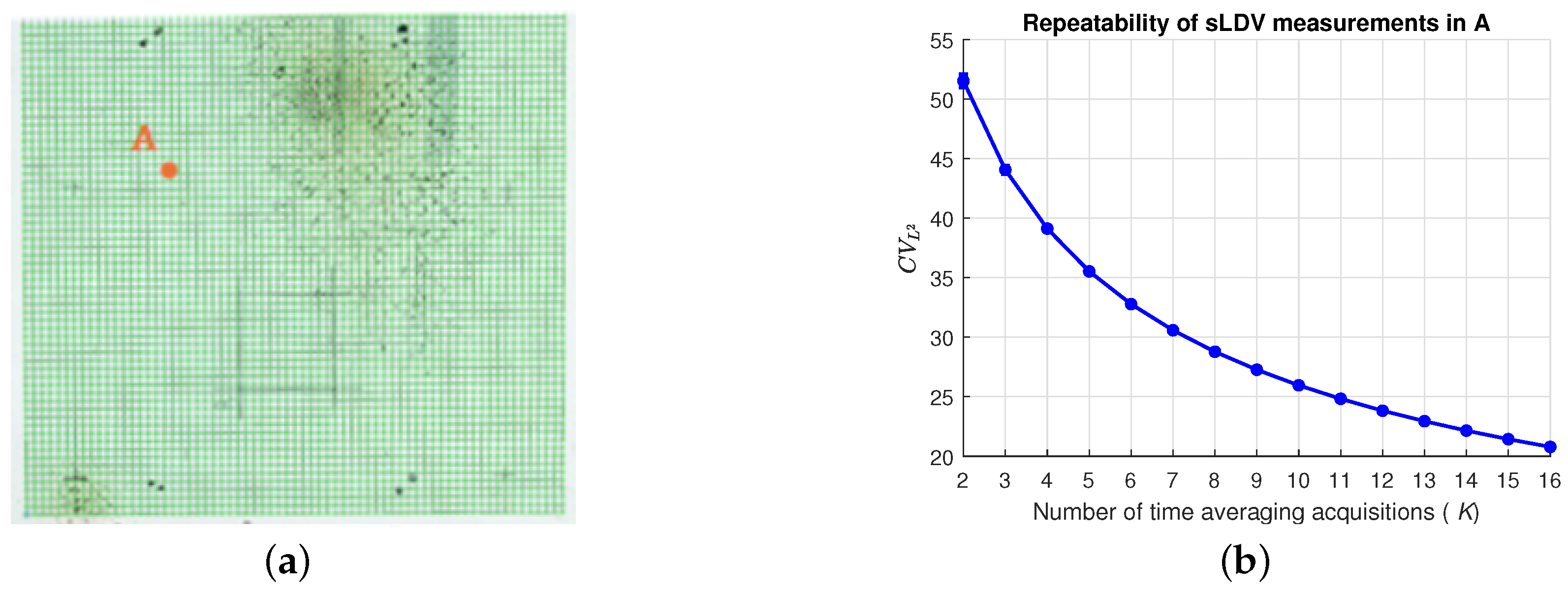
The remainder of this paper is organized as follows. In Section 2 the GFRP specimen and the measurement setup are described, including a description of other composite panels inspected to test the methodology sensitivity, while in Section 3 two defect detection algorithms belonging to LWE family are presented: one based on the SSFT and the second based on 2D-CWT. In Section 4, the results corresponding to the two wavenumber imaging algorithms are shown and compared to two techniques based on simple RMS values, evaluating their performance through blob analysis measures. In addition, a repeatability analysis of the provided impulsive signal is performed. Section 5 summarizes the work conclusions in terms of scope of the work, implemented methodology, results and considerations about future research path.

2. Experimental Setup

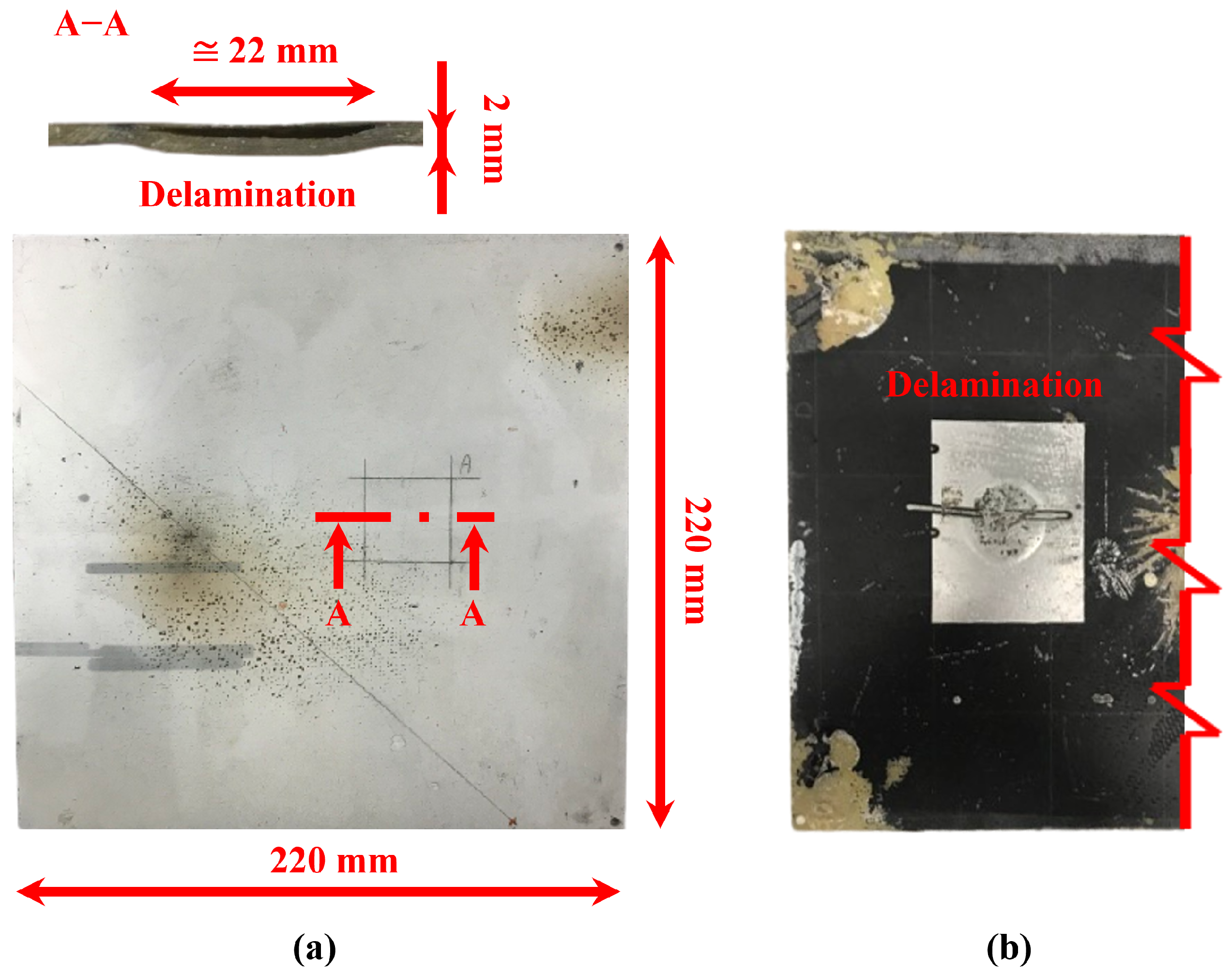
The specimen considered in this study, consisting of a flat GFRP panel, has already been described in previous works [34,35,36,37]. It has a 2 mm thickness consisting of 7 layers of canvas immersed in a matrix of epoxy resin. The defect is obtained by introducing, between layers 3–4 a wax disc of diameter of 22 mm in known positions during the lamination procedure. The wax is removed by heating the solid epoxy matrix through the panel porosity, in such a way to create empty cavities between the layers. The front and back side of the GFRP plate are shown, respectively, in Figure 1a,b, along with dimensional details and a cross-sectional view of the artificial delamination. This type of delamination simulates real defects that can rise during the production of the object (low pressure, absence of resin, presence of foreign matters, etc.). As can be deduced from Section 1, this is a straightforward case, exploited in this work to compare the proposed, different methods.

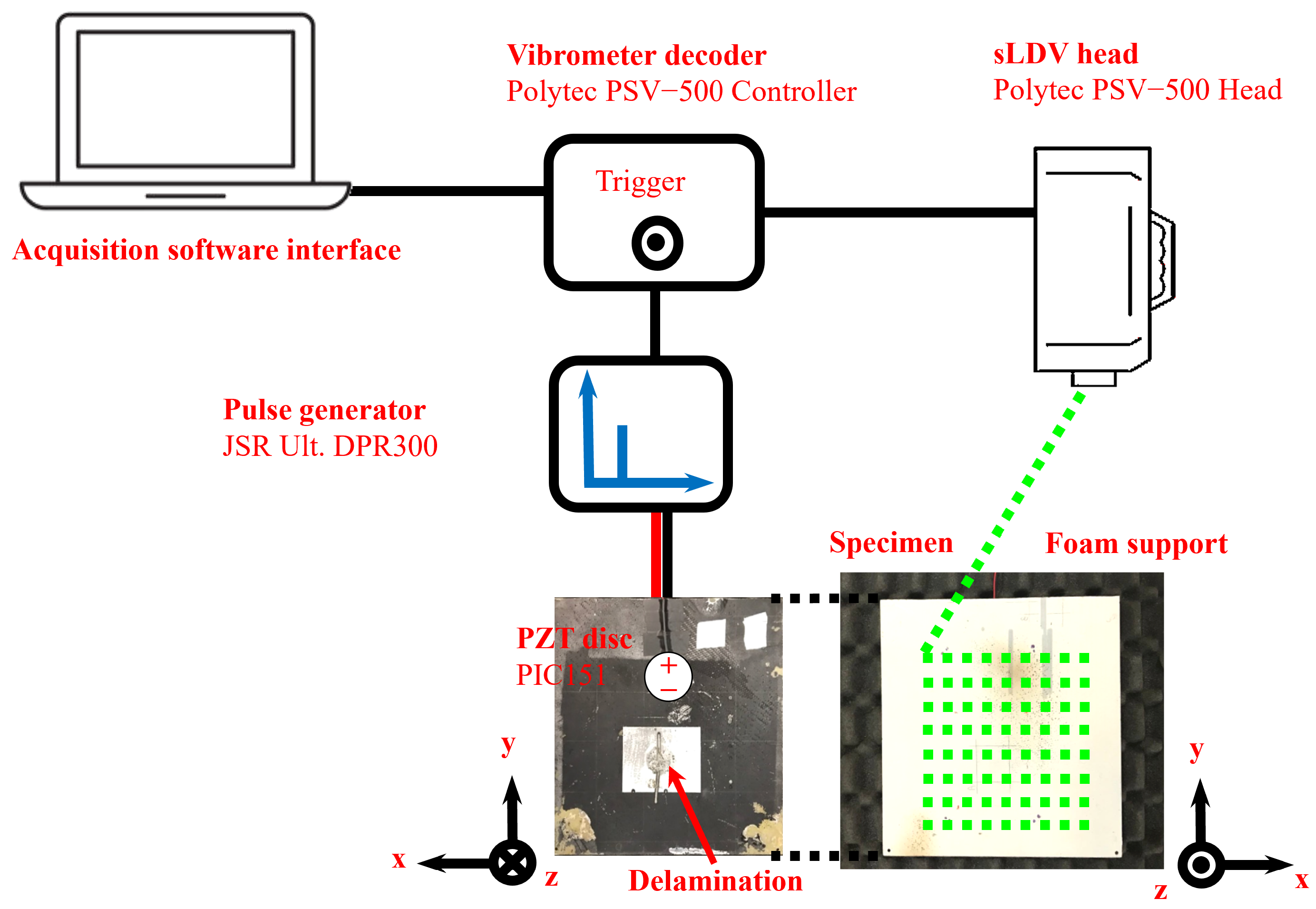
The specimen is placed on top of foam rubber to simulate a free-free boundary condition, avoiding any fixed constraint which could compromise free wave propagation. Moreover, the plate has been excited by an impulsive signal through a 10 mm diameter piezoelectric actuator disc installed in the opposite surface, with respect to the one on which vibrational measurements are carried out, by means of an epoxy resin. Acquired data, which consist in out-of-plane velocity v, has been obtained by means of a scanning SLDV over a 64 × 64 scanning grid with spatial resolution of about 1.9 mm. Measures are taken sequentially point-by-point and, therefore, also the excitation signal is repeated at each measurement point of the scanning grid (i.e., 64 × 64 times). Therefore, the resulting data is a 4-D matrix having the velocity value at each grid point location $(x,y)$, at each acquired time step. The testing setup is shown in Figure 2.

The generated Lamb waves have been observed through a single point Laser Doppler Vibrometer from Polytec (Waldbronn, Germany), consisting of the laser head (model OFV-505) and the controller (model OFV 5000 controller). The laser beam has been made to move through the defined points grid on the structure by a 2 axis motorized stage. The acquisition parameters are synthesized in

Table 1. Acquisition settings.

$F_s$	250 kHz	Sample frequency
$F_b$	100 kHz	Frequency bandwidth
T	10 ms	Acquisition time
n	16	Time averages per point
N	67	X-axis grid points number (the same for Y-axis)
$\Delta$	1.9 mm	Spatial resolution along x-axis an y-axis

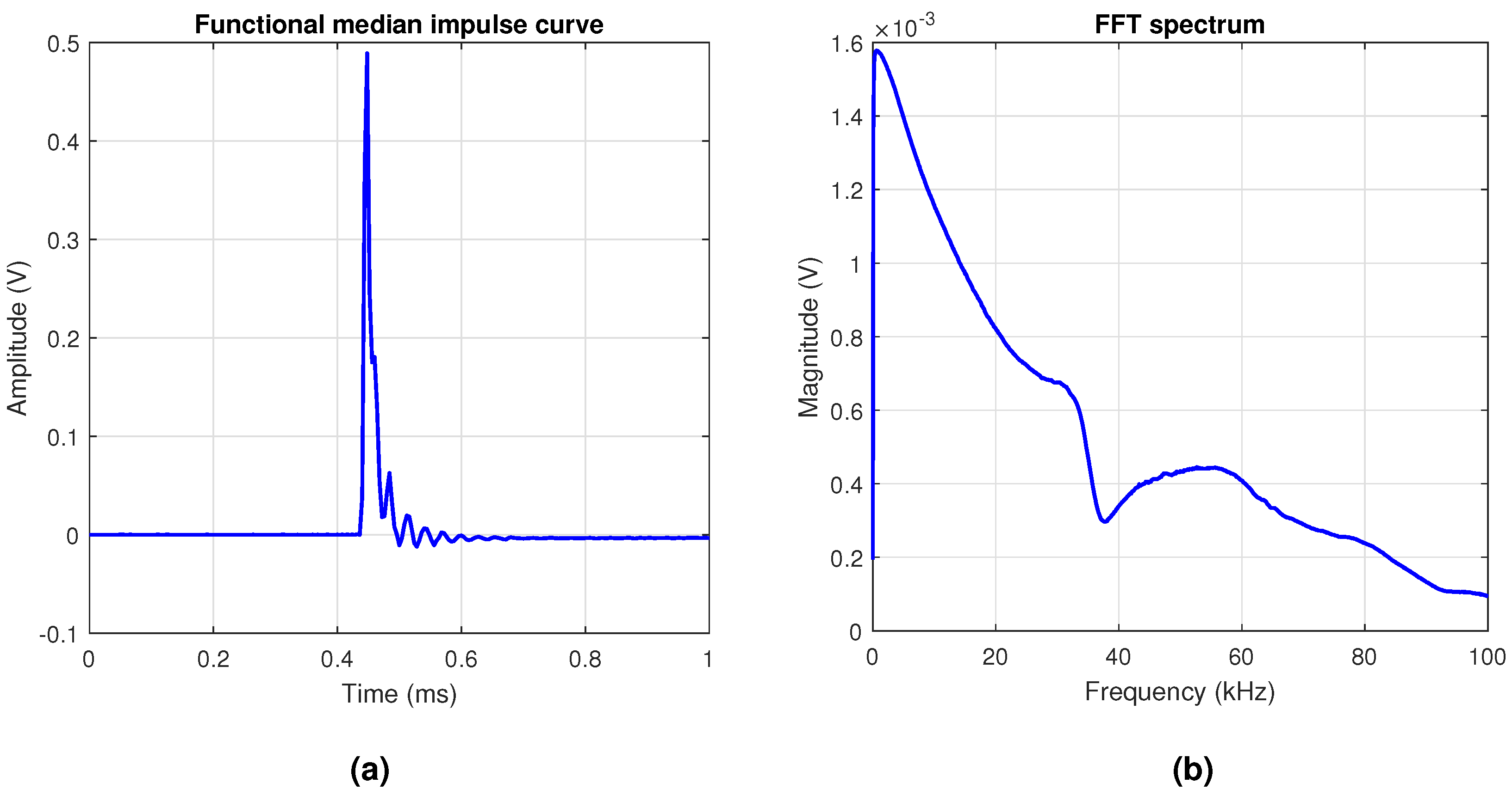
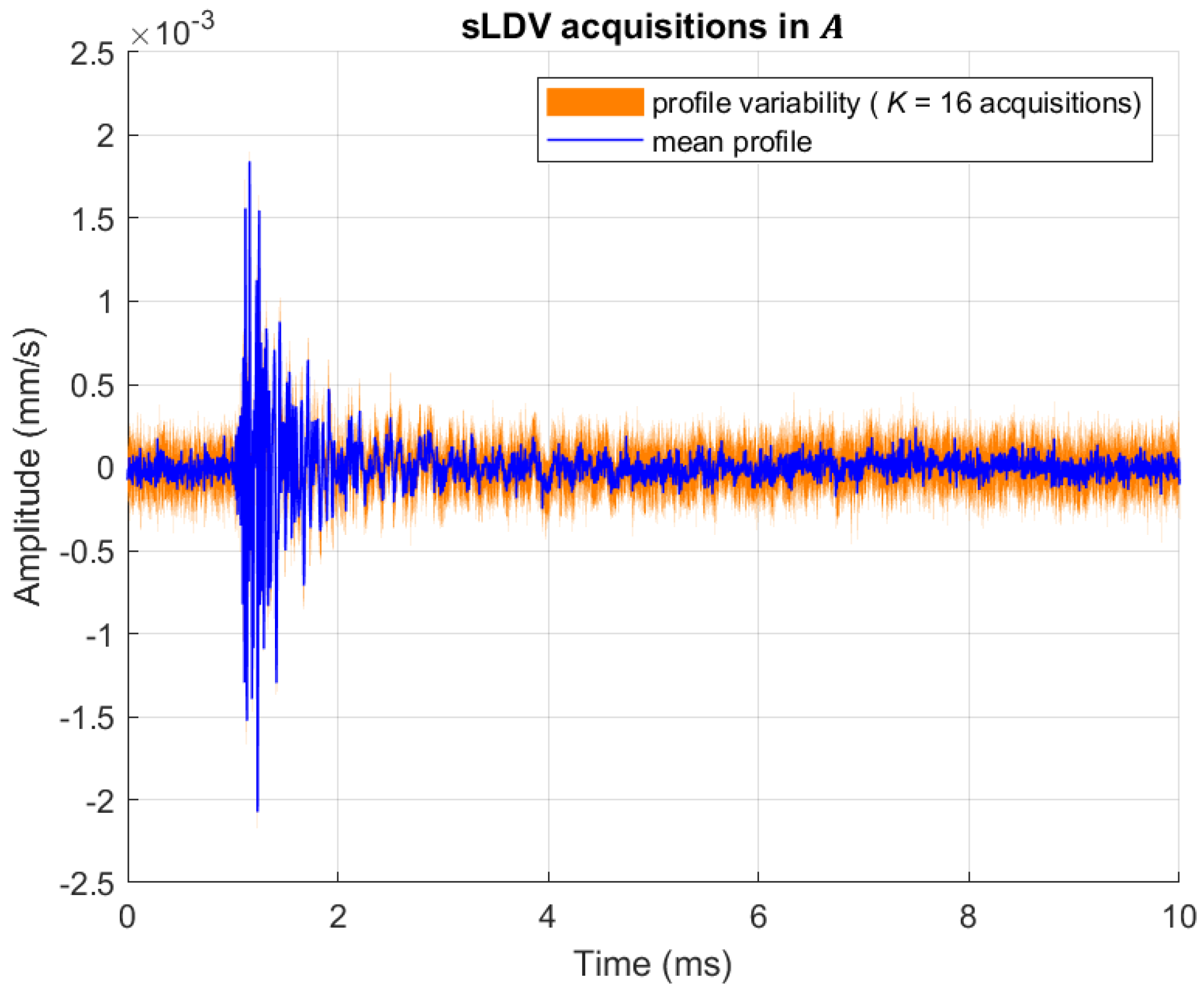
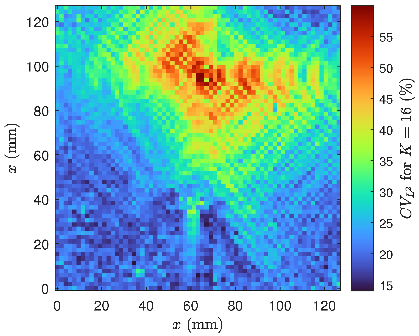
: the sample frequency and the acquisition time at each spatial position have been set to 250 kHz and 10 ms, respectively. The LDV velocity decoding sensitivity has been set to 2 (mm/s)/V [37]. For each spatial position, 16 time histories have been acquired for averaging purpose to improve SNR. The vibrometer has been fixed using a proper structure with high stiffness to minimize vibrations, and assuring the laser beam to be exactly orthogonal to the specimen surface. The distance between the lens and the target has been set at about 64 cm. An impulsive excitation signal is sent to the specimen by means of the pulse generator JSR Ultrasonics DPR 300 (Pittsford, NY, USA), which has been used to trigger the velocity time signals acquisition as well. The pulse is defined in terms of amplitude (V), duration (ms) and PRR (Hz). To evaluate these parameters, the functional median time profile was extracted from the entire set of acquired excitation signals, along with its spectrum, which are depicted, respectively, in Figure 3a,b. The amplitude of the functional median pulse profile is 0.49 V, and its duration according to the mid-reference level crossings of the first and second transitions is 23 $\mu$s. The PRR has been set to 100 Hz. This value assure the wave propagation has ceased reaching background noise level due to damping within each pulse and, therefore, pulse overlapping is avoided. This assumption has been previously verified considering the time domain amplitude signal decay.

3. Damage Detection Procedure Based on Wavenumber Imaging

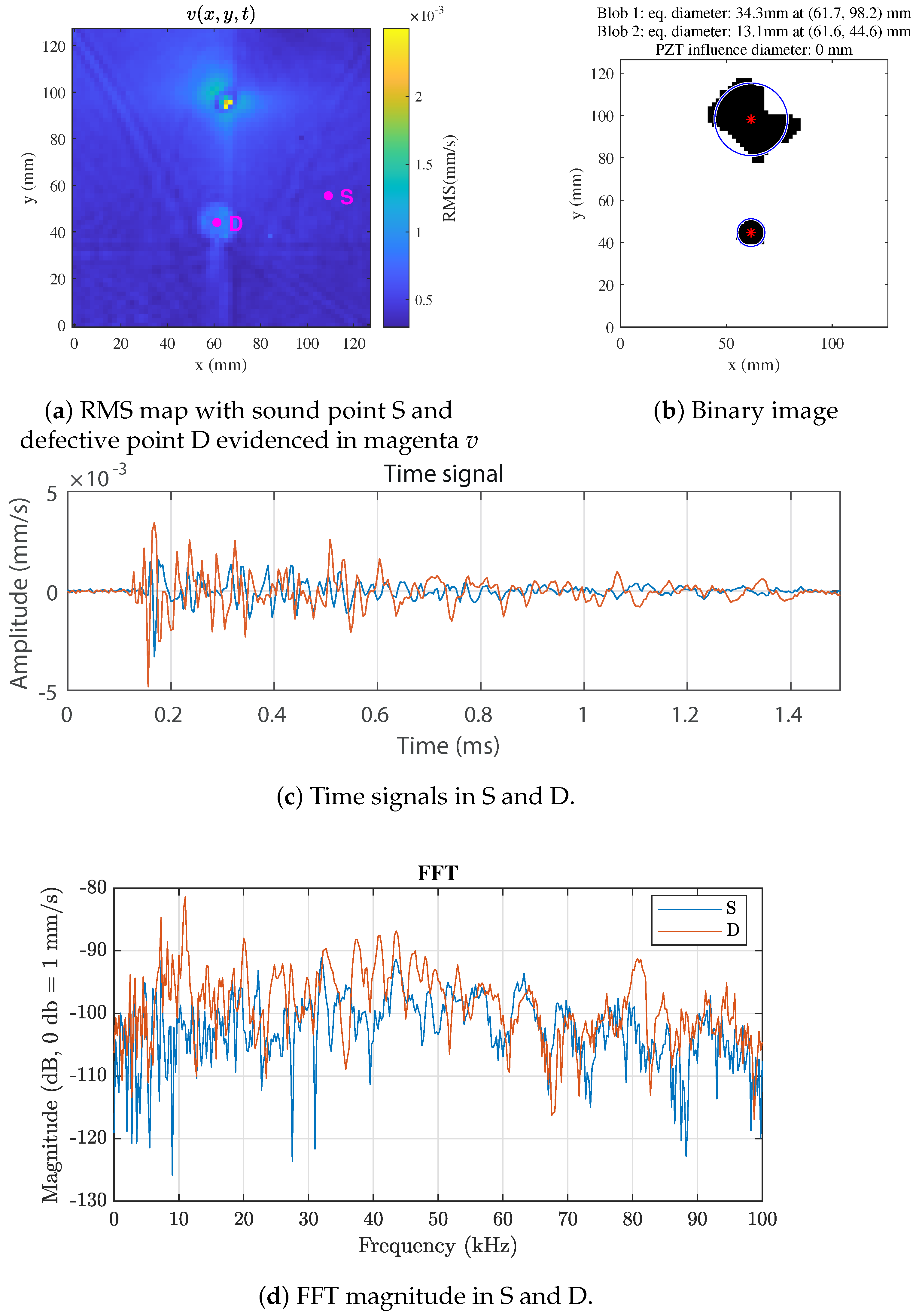
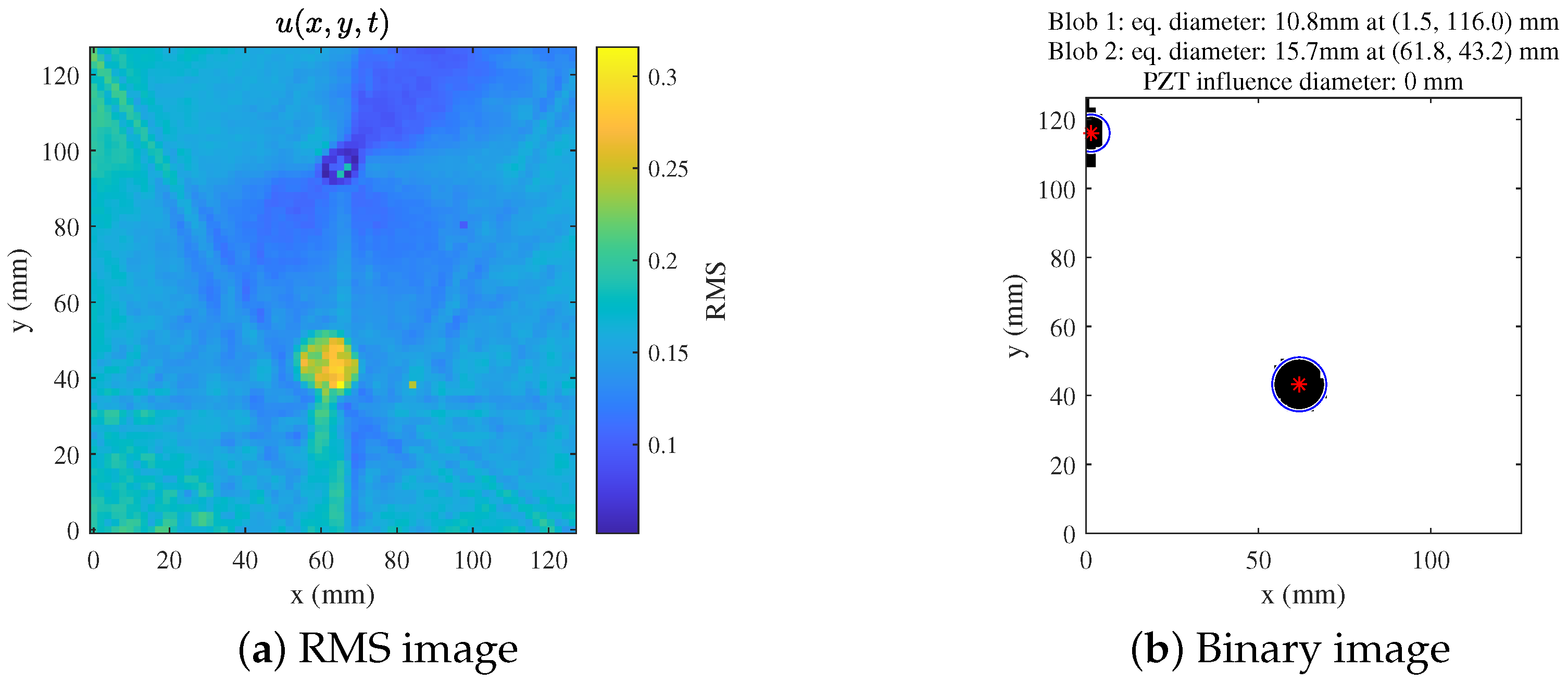
Lamb waves passing through defects, such as delamination in composite materials, have the dual effect of increasing the vibration amplitude and changing the propagation velocity due to thickness reduction [10]. However, a simple RMS analysis is only capable of distinguishing the intact region from the delaminated area with low contrast, returning an image significantly affected by waves interactions with the panel boundaries.

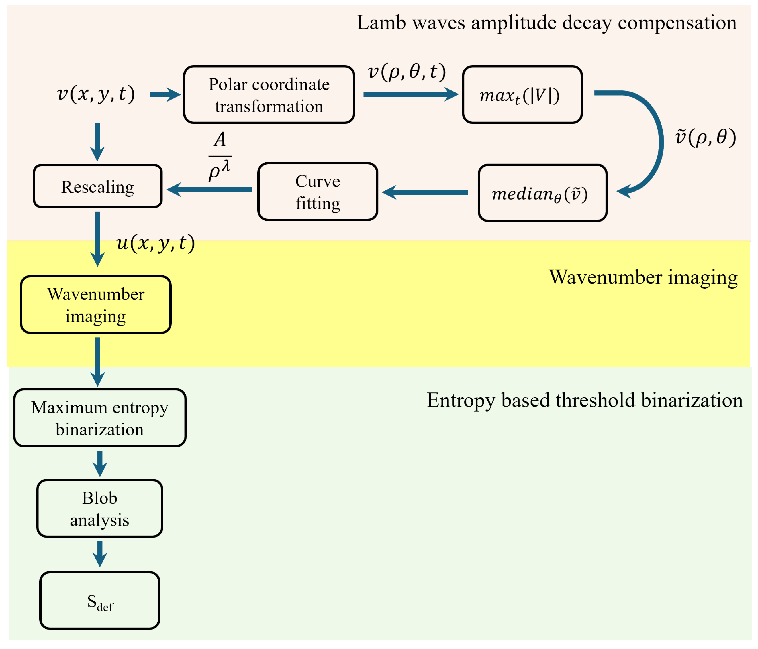
The proposed defect detection framework is based on wavenumber imaging exploiting the difference between the mean elastic wavelength crossing the defective region with respect to the intact surface. Its flowchart is shown in Figure 4. The framework is divided in three phases: (i) a preprocessing phase where the measured velocity signals are scaled to compensate the Lamb waves amplitude decay (the followed procedure is explained in Section 3.1), (ii) the core phase where the wavenumber imaging is performed, as described in Section 3.2, (iii) the final phase involving the image binarization and defect features extraction detailed in Section 3.3.

The wavenumber imaging technique analyzed consists of the LWE method [29]. The diagnostic principle of this method relies that defects like delamination effectively split the laminate into sub-layers, they cause a local reduction of effective thickness and hence flexural stiffness. 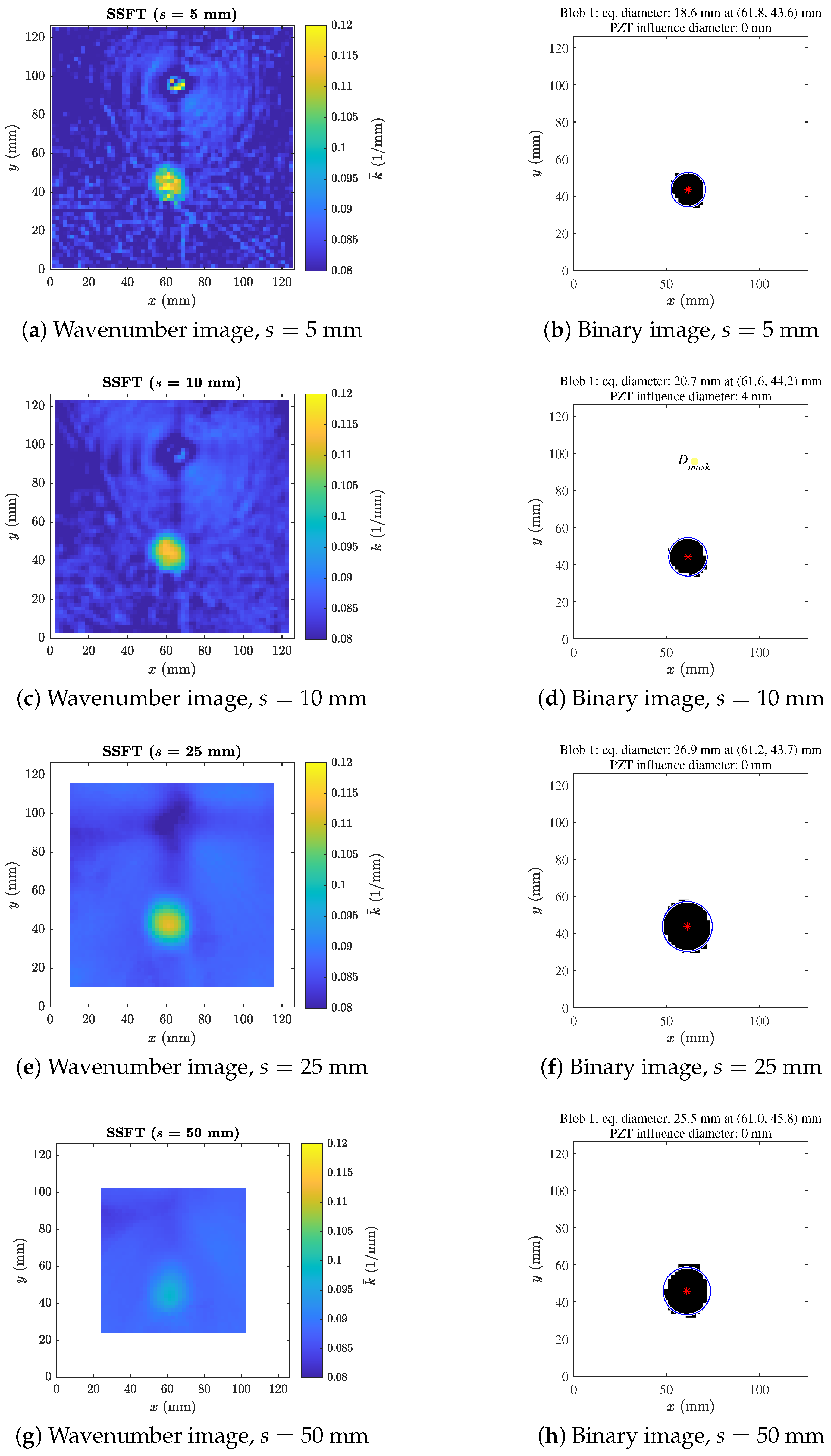According to Lamb wave dispersion relations, this reduction alters the frequency-thickness product, typically resulting in higher wavenumber values within the damaged region compared to the intact plate [38]. Consequently, a delamination appear as a contrasted region in the wavenumber images respect the surrounding intact material. LWE is performed through the two alternative methods: SSFT and 2D-CWT. SSFT based method is the standard in LWE technique and requires as input the size of a spatial window, which is a parameter that depends on the maximum tolerated dimension, but affects wavelength resolution. This naturally implies that a poorly configured spatial window can significantly compromise detection performance. Specifically, selecting a spatial window that is excessively large compared to the defect dimensions leads to a lower defect-to-background contrast, where the local wavenumber assigned to a point involved by the defect is weakened by the dominant wavenumber contribution of the surrounding, intact material. This results in a loss of spatial localization and a potential underestimation of the defect’s presence, as the “smearing” effect involved obscures the boundaries of the damaged area. Conversely, if the spatial window is too small, the resolution in the wavenumber domain degrades: a spatial window $M\times M$ corresponds to a wavenumber image with insufficient resolution thereby reducing again the defect-to-background contrast below the level required for reliable identification of the delaminated area. The 2D-CWT effectively circumvents these limitations through its inherent multiscale analysis capabilities. By projecting the wavefield onto a family of wavelets originated from a suited mother wavelet, the 2D-CWT simultaneously interrogates the signal across a continuous range of spatial scales. Although the spatial scale parameter of a wavelet does not directly represent a wavenumber from a strict metric standpoint, the two quantities are intrinsically and mathematically related: the scale dictates the spatial spectral extension of the wavelet, which is inherently characterized by a principal central wavenumber. Because the proposed method identifies the dominant spatial scale and averages this pseudo-wavenumber feature across the frequency band, it conceptually mirrors conventional Local Wavenumber Estimation approaches while operating in the scale domain. This eliminates the need for a priori selection of a fixed window size. Instead of iteratively executing the SSFT at multiple spatial window sizes, which would increase computational cost, the 2D-CWT identifies the optimal scale that maximizes the wavelet coefficient at each spatial coordinate in a single processing pass. This allows a dynamic adaptation to the local feature size, ensuring robust defect localization and sizing without the redundancy of multiple fixed-window analyses. of the proposed LWE algorithms include a pre-processing phase at wavenumber imaging to compensate for the attenuation of elastic waves. Downstream, a segmentation phase of the binary image is exploited to extract the defective area of any detected defects. The wavenumber images resulting from the two methods are compared through IoU metric of the extracted binary blobs, considering the ground truth defect information. Each signal processing phase is described below.

3.1. Lamb Waves Amplitude Decay Compensation

The fundamental rule states that the magnitude of Lamb waves in a plate decays at a rate proportional to the inverse square root of the propagation distance [39]. This attenuation is primarily caused by the geometrical spreading of the elastic wavefronts. Beyond geometric spreading, Lamb waves attenuation is heavily influenced by:

• wave mode: the attenuation can differentiate between symmetric $S_i$ and anti-symmetric $A_i$ modes [39].
• material properties and structure: it has been observed that waves propagate relatively farther in carbon CFRP than in GFRP [12,39]; damage such as delamination or rivet holes increases dissipation (e.g., it was observed that 52% of the total energy dissipates when a Lamb wave passes through a damage area of 7 mm in diameter in a composite laminate [39]).
• acoustic impedance boundaries along the wave propagation path: the elastic wave intensity is redistributed according to energy partitioning via reflection and transmission phenomena. A significant portion of the wave energy is reflected backward by the geometric boundaries of the structure rather than transmitted into the environment. This reverberation maintains a higher local energy density with respect to free field propagation reducing the attenuation coefficient (this effect is described considering the boundaries of a delamination in respect with the intact surrounding material [40]). This phase addresses the attenuation of Lamb waves as they propagate outward from the excitation source. The measured out-of-plane velocity $v(x,y,t)$ is processed to compensate the amplitude decay through a modelled isotropic decay function.

This process involves two steps:

1.

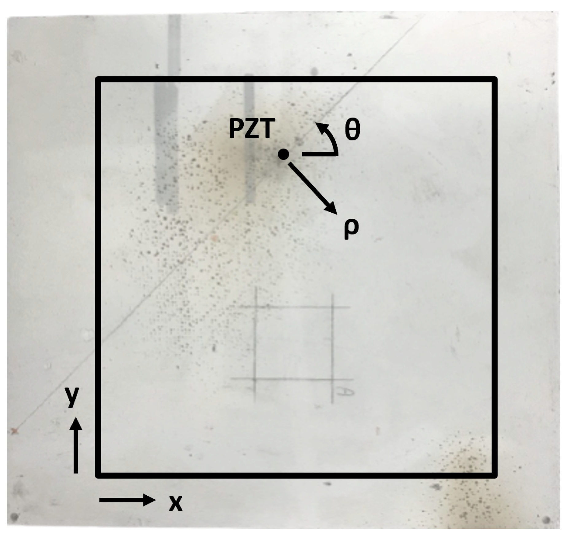
Decay modelling: the measured velocity $v(x,y,t)$ is transformed in polar coordinate with the centre of the reference system coinciding with the point on measurement surface corresponding to the PZT disc centre: $v(\rho ,\theta ,t)$. The acquisition surface, including the localization of the piezoelectric disc center and the coordinate systems employed is illustrated in Figure 5.

The maximum local response $\tilde{v}$ generated by the propagating Lamb wave packet is extracted by applying the following equation:

$$\tilde{v}(\rho ,\theta )=\underset{t}{\max }\left|v(\rho ,\theta ,t)\right|$$

(1)

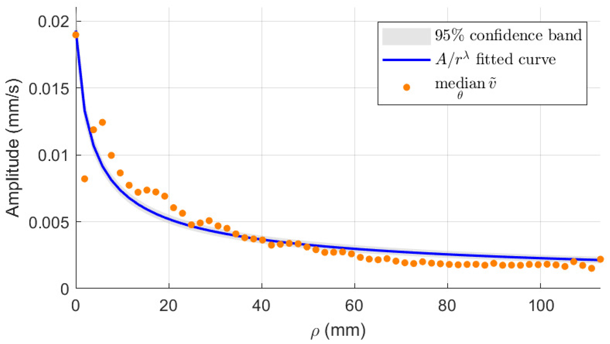
The median amplitude profile ($\underset{\theta }{median}\tilde{v}$) along the radial direction $\rho$ is fitted to capture the baseline attenuation of the intact plate, using the decay model:

$$D\left(\rho \right)={\displaystyle \frac{A}{{\rho }^{\lambda }}}$$

(2)

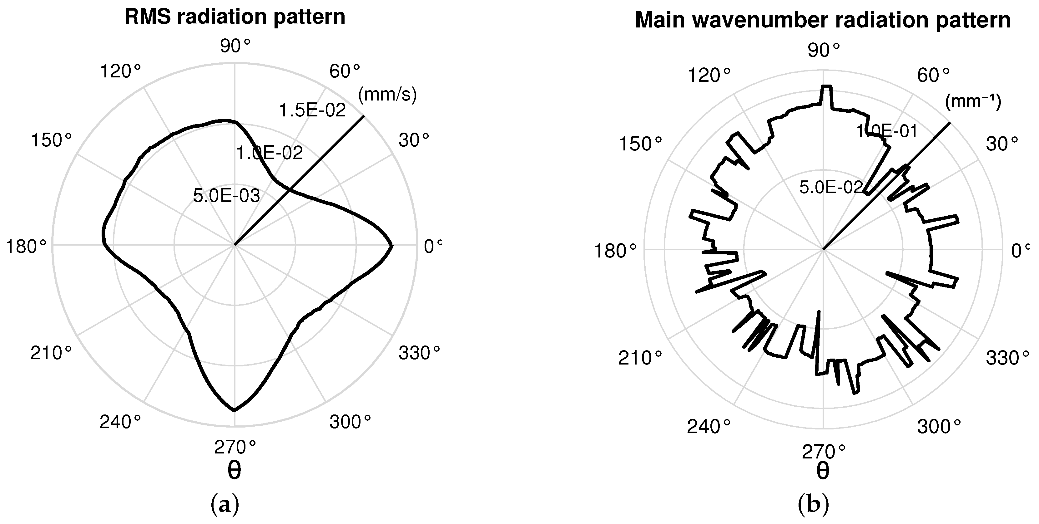
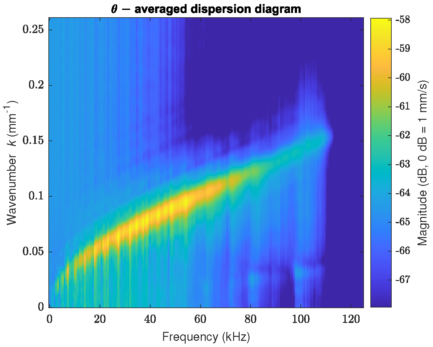
with parameters $A,\lambda$ as shown in Figure 6. Curve fitting is performed through non-linear least square minimization. Equation (2) assumes an isotropic wave propagation behavior. However, the tested GFRP plate exhibits anisotropic behavior in terms of propagating wave intensity and dominant wavenumber content, as shown in Figure 7.

While the described pre-processing step is a simplification of the anisotropic nature of composite materials, it improves the robustness of the attenuation estimation, at the expense of collapsing the spatial variability into a single radial line due to the median operation across all angular directions. Another simplification lies in the assumption of uniform surface roughness, thereby neglecting local variations that may arise from localized wear induced by concentrated loads and cause different attenuation decay. The choice of using a non-linear optimization over log-space linearization least square minimization is driven by the standard hypothesis that noise in ultrasonics waves propagation is typically additive [41]. Consequently, high-amplitude data points near the source possess a significantly higher Signal-to-Noise Ratio than low-amplitude points in far-field. Transforming data into log-space alters the error distribution. Due to Jensen’s inequality [42] regression in log-space converges to the geometric mean of the data, systematically lower than the arithmetic mean. Therefore, log-linear least square based fitting would have resulted in an underestimation of the decay. The solver adopted is the Trust-Region-Reflective [43] using as parameters space starting point the following ones:

$$\left\{\begin{array}{c}{A}_0=\tilde{v}{|}_{\rho =0},min\left\{\underset{\theta }{median}\tilde{v}\right\}\le A\le max\left\{\underset{\theta }{median}\tilde{v}\right\}\hfill \\ {\lambda }_0=0.5,\lambda >0\hfill \end{array}\right.$$

(3)

The amplitude coefficient $A_0$ is initialized with the observed signal intensity at the source, and the tentative decay exponent ${\lambda }_0$ is evaluated according to the geometric spreading of Lamb waves. To quantify the overall uncertainty of the fitted regression $u_D$, a $95\%$ confidence band was calculated for the decay model in Equation (2). The boundaries were derived by propagating the parameter uncertainties from the covariance matrix of the non-linear least squares fit, utilizing the Student’s t-distribution evaluated at $N_{\rho }-2$ degrees of freedom, where $N_{\rho }$ is the number of radial positions.

2.

Signal rescaling: an amplitude-compensated signal $u(x,y,t)$ is generated by dividing the original velocity signal by the fitted decay model $D\left(\rho \right)$ (in Equation (2)) back-transformed in Cartesian coordinates ($D(x,y)$):

$$u(x,y,t)={\displaystyle \frac{v(x,y,t)}{D(x,y)}}$$

(4)

3.2. Wavenumber Imaging

Two distinct methods are implemented to convert the amplitude compensated time-domain data $u(x,y,t)$ into wavenumber maps, beyond the simple RMS imaging: SSFT and 2D-CWT. Phase information is not considered in both approaches in order to ease the signal processing pipeline. As a consequence to this simplification, a loss of information may happen regarding relevant wave propagation characteristics. Nevertheless, the amplitude was selected because it provides a robust and physically meaningful indicator of wave energy concentration, which is the primary quantity of interest for the proposed damage detection methodology.

3.2.1. Wavenumber Imaging Based on SSFT

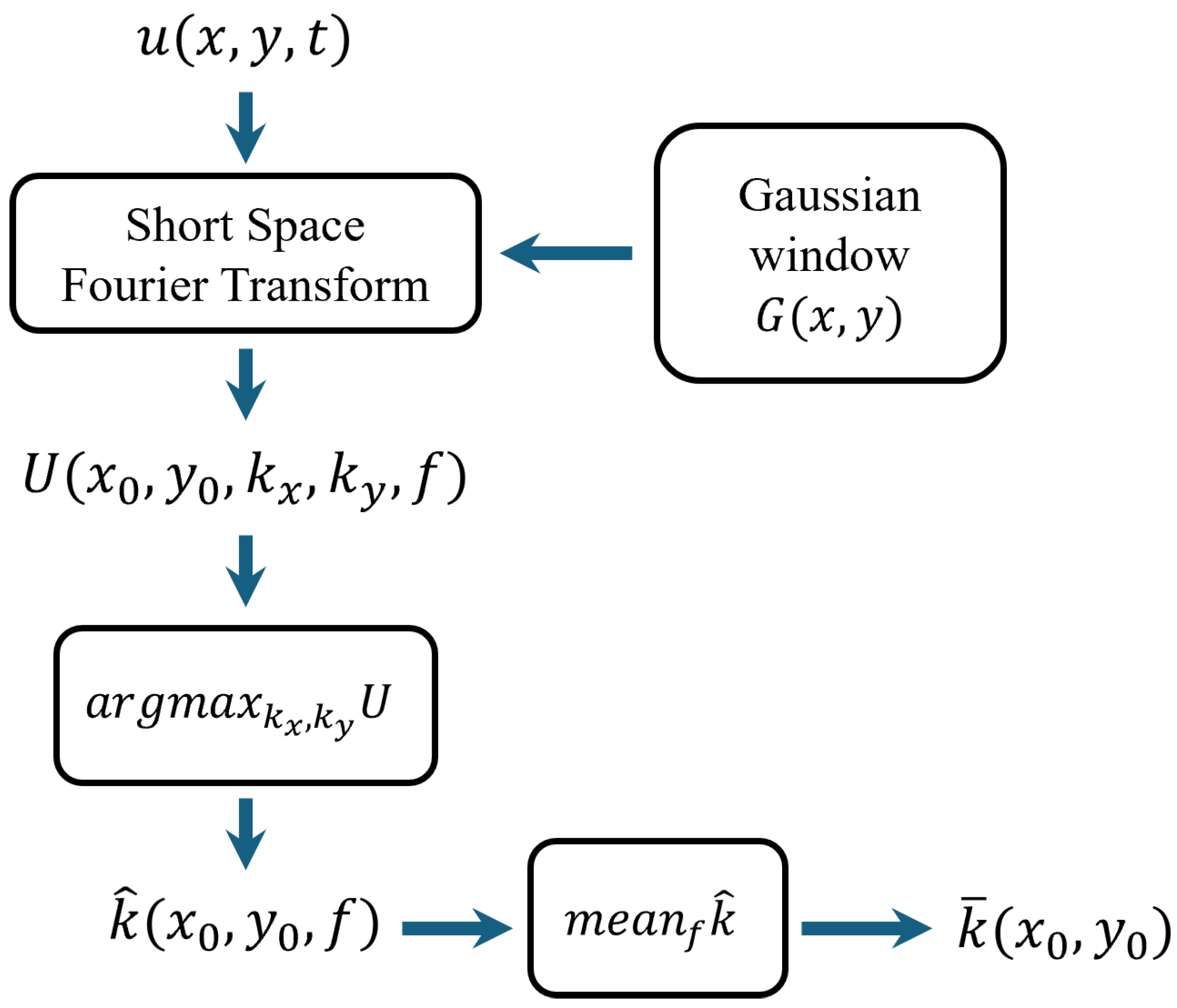
The wavenumber image extraction procedure is illustrated in the flowchart reported in Figure 8. As a first step, a 3D Fourier transform is applied to convert the scaled velocity signal $u(x,y,t)$ into the wavenumber-frequency domain ($U(k_x,k_y,f)$), according to established approaches in the literature (e.g., [26]), as expressed in the following equation:

$$U({\mathbf{x}}_{\mathbf{0}},\mathbf{k},f)=\sum _t\sum _{\mathbf{x}}u(\mathbf{x},t)G(\mathbf{x}-{\mathbf{x}}_{\mathbf{0}})e^{-2\pi j(ft+\mathbf{k}·\mathbf{x})}$$

(5)

where $\mathbf{x}=(x,y)$ is the space vector, ${\mathbf{x}}_{\mathbf{0}}$ the spatial lag in the same $\mathbf{x}$ domain and $\mathbf{k}=(k_x,k_y)$ is the wavenumber vector. $U({\mathbf{x}}_{\mathbf{0}},\mathbf{k},f)$ is the resulting spectrum, and $G(\mathbf{x}-{\mathbf{x}}_{\mathbf{0}})$ is a Gaussian sliding fixed-size window function as defined in the following equation:

$$G\left(\mathbf{x}\right)=e^{-{\displaystyle \frac{{\mathbf{x}}^2}{2s^2}}}$$

(6)

having standard deviation s and centered at position ${\mathbf{x}}_{\mathbf{0}}=(x_0,y_0)$. U depends on the extent M of the window itself related to its standard deviation value s. We have considered the sliding window extension of size M pixels as the square bounding box that contains $95\%$ of the unit volume subtended by G. Starting from the spectral representation $U(x_0,y_0,k_x,k_y,f)$, defined at each spatial position $(x_0,y_0)$ and frequency f, the algorithm first search for the maximum U in the $(k_x,k_y)$ domain, which yields the estimated wavenumber vector $\widehat{k}(x_0,y_0,f)$. Subsequently, the estimated wavenumber $\widehat{k}(x_0,y_0,f)$ is averaged over the frequency dimension. This frequency-wise mean operation produces a single representative wavenumber value $\overline{k}(x_0,y_0)$ for each spatial location, which represents the local wavenumber content across the considered frequency range. The spatial map of the mean wavenumber $\overline{k}(x_0,y_0)$ depends on the size s of the Gaussian sliding window trough Equation (5), imposing a fundamental trade-off. If s is chosen small enough, G decays rapidly and severely truncates the spatial summation. This make the computation of U highly susceptible to the signal noise around ${\mathbf{x}}_{\mathbf{0}}$. Conversely, if s is very large, $G\approx 1$, driving U to be independent of ${\mathbf{x}}_{\mathbf{0}}$, and therefore the wavenumber localization capability is reduced. Equation (5) is computed numerically via the Fast Fourier Transform algorithm, the spectrum is inherently evaluated over a discrete wavenumber array $\mathbf{k}$. The resolution of this rectangular k-space grid is defined as $\delta k=2\pi /(M\Delta )$. When M is small enough the coarse k-space discretisation introduces a severe directional bias in the spectral peak estimation. According to the Fourier rotation theorem, a plane wave propagating at angle $\theta$ produces a spectral magnitude peak at the same $\theta =\arctan (k_y/k_x)$ in k-space; yet, on a discrete rectangular grid, only angles for integer pairs are representable. For a window $3\times 3$ pixels, for instance, only $0^{\circ }$, ${45}^{\circ }$, and ${90}^{\circ }$ exist on the grid. Consequently, waves propagating at intermediate directions are systematically misrepresented, introducing a severe bias on the estimated propagation direction of the dominant wavenumber. To ensure a fair and consistent comparison between the wavenumber images obtained via SSFT at different s values, and to effectively remove this directional artefact, each windowed signal block is spatially zero-padded to the full scanning grid extent $N\times N$ prior to computing the FFT. This operation yields a uniform wavenumber resolution $\delta k=2\pi /(N\Delta )$ for all evaluated window sizes. After zero-padding any residual differences between the maps evaluated at various window sizes are no longer numerical artefacts, but are entirely attributable to the fundamental spatial resolution–wavenumber resolution trade-off that is intrinsic to the SSFT. Since the wavenumber value assigned to each spatial location ${\mathbf{x}}_{\mathbf{0}}$ is computed by centering the sliding Gaussian window G exactly on that coordinate, the window inevitably extends beyond the physical boundaries of the acquired scan grid when evaluating points near the edges. To avoid spectral artifacts caused by this lack of spatial data, we cropped the resulting wavenumber image at the borders by a margin equal to the integer part of half the window size $⌊{\displaystyle \frac{s}{2}}⌋$.

3.2.2. Wavenumber Imaging Based on 2D-CWT

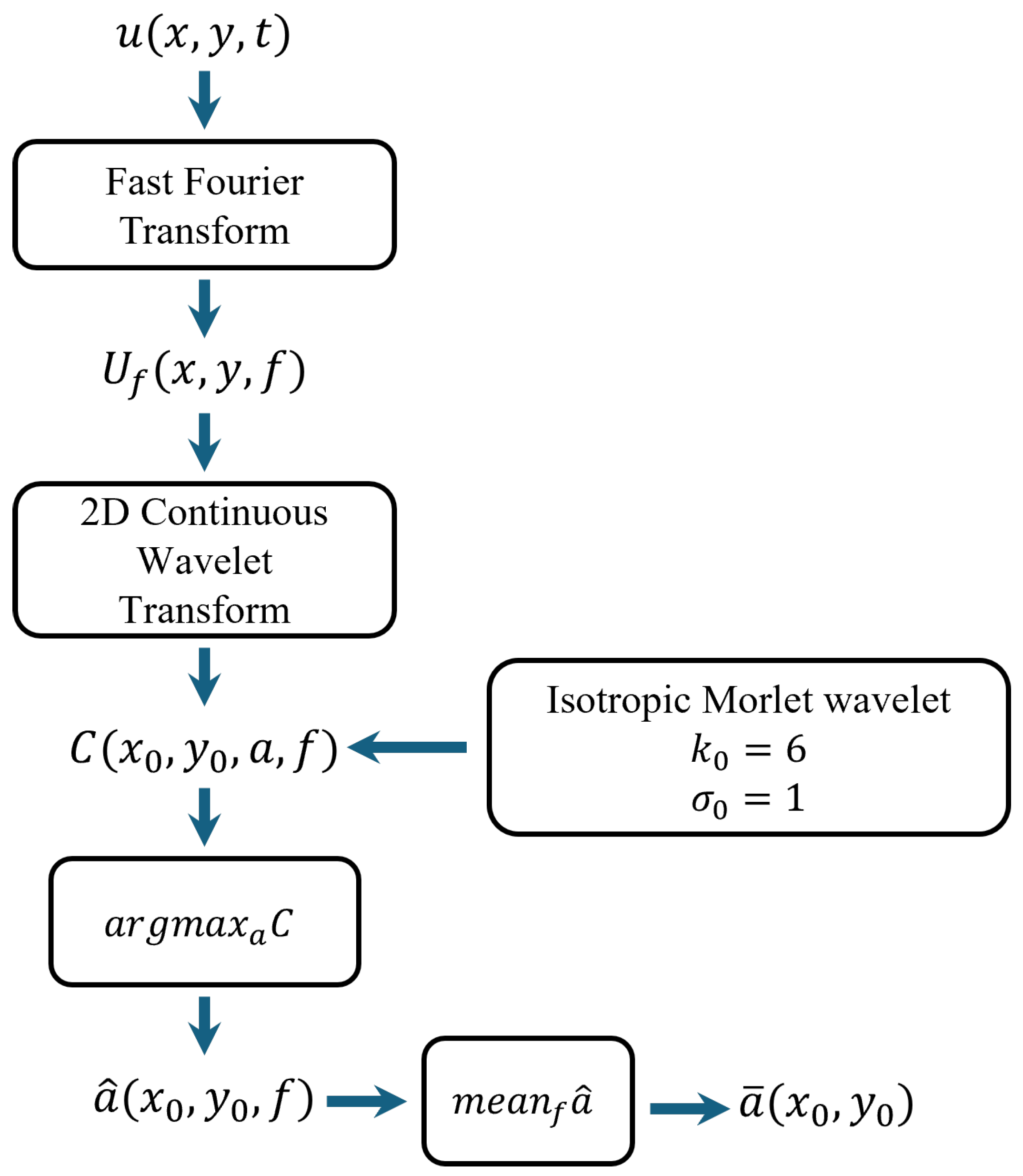
The flowchart of the proposed wavenumber imaging method is shown in Figure 9. Firstly, the algorithm involves a Fourier Transform in the time domain of the scaled velocity signal $u(x,y,t)$, as already done in Section 3.2 for the SSFT wavenumber imaging:

$$U_f(\mathbf{x},f)=\sum _{t}u(\mathbf{x},t)e^{-j\left(2\pi ft\right)}$$

(7)

In order to perform a ‘multi-size’ analysis, avoiding the redundancy of performing SSFT (Equation (5)) at different s, a 2-dimensional wavelet support defined in $\mathbf{x}$ is configured. The eligible wavelet should have the following characteristics:

1.

it needs to be axisymmetric in order not to have certain preferred directions of sensitivity since the defect geometry and its effect in wave propagation are unknown. Directional wavelets, such as the anisotropic real Morlet wavelet, can be advantageous when the orientation of damage-induced wave-scattering features is known in advance, since the wavelet selectively amplifies energy propagating along a prescribed direction. An omnidirectional aggregation over all rotation angles, as proposed in [44] would recover the defect but at the cost of re-introducing the isotropic character of the transform and multiplying the computational burden by the number of discrete angles. The isotropic Morlet wavelet therefore remain preferable for a blind inspection scenario, as it provides uniform sensitivity to damage regardless of its spatial orientation, without requiring prior knowledge of the defect geometry.

2.

it minimizes overall uncertainty $u_{\alpha }(k,{\mathbf{x}}_{\mathbf{0}})$ in detecting a certain wave number modulus $k=\sqrt{k_x^2+k_y^2}$ that occurs at position ${\mathbf{x}}_{\mathbf{0}}$, when choosing a confidence level $\alpha$.

A straightforward consequence of the first characteristic is that only a purely real function can be chosen since its phase must be constant along $\theta$. Considering the second characteristic, since Schwarz’s covariance theorem holds, it implies $u_{\alpha }{(k,{\mathbf{x}}_{\mathbf{0}})}^2\le u_{\alpha }\left(k\right)u_{\alpha }\left({\mathbf{x}}_{\mathbf{0}}\right)$. $u_{\alpha }\left(k\right)$ and $u_{\alpha }\left({\mathbf{x}}_{\mathbf{0}}\right)$ are related from Gabor uncertainty principle $u_{\alpha }\left(k\right)u_{\alpha }\left({\mathbf{x}}_{\mathbf{0}}\right)\ge {\displaystyle \frac{1}{2}}$. The result is finding a 2D wavelet that allows a constant uncertainty function: $u_{\alpha }={\displaystyle \frac{1}{2}}$. From [45] it can be shown that a wavelet that satisfies both conditions is the isotropic Morlet wavelet (also known as “Halo” wavelet):

$${\psi }_M\left(\mathbf{x}\right)=\cos (k_0\left|\mathbf{x}\right|)e^{-{\displaystyle \frac{{\mathbf{x}}^2}{2{{\sigma }_0}^2}}}$$

(8)

$${\widehat{\psi }}_M\left(\mathbf{k}\right)={\displaystyle \frac{1}{2{\sigma }_0^2}}{e}^{-{\displaystyle \frac{\left(\right|\mathbf{k}|-k_0{)}^2}{2{\sigma }_0^2}}}$$

(9)

where $k_0$ is the central spatial frequency of the wavelet, ${\sigma }_0$ the standard deviation of the Gaussian envelope and the size of the mother wavelet support ${\psi }_M$. The isotropic Morlet wavelet is chosen over a classical directional Morlet wavelet as it allows to reduce the set of parameters under investigation. In fact, as the location of the defect is unknown, the wavenumber direction to be considered is also unknown. Therefore, considering a directional wavelet means adding a further parameter and investigating every possible propagation direction, which results in higher computational costs and time.

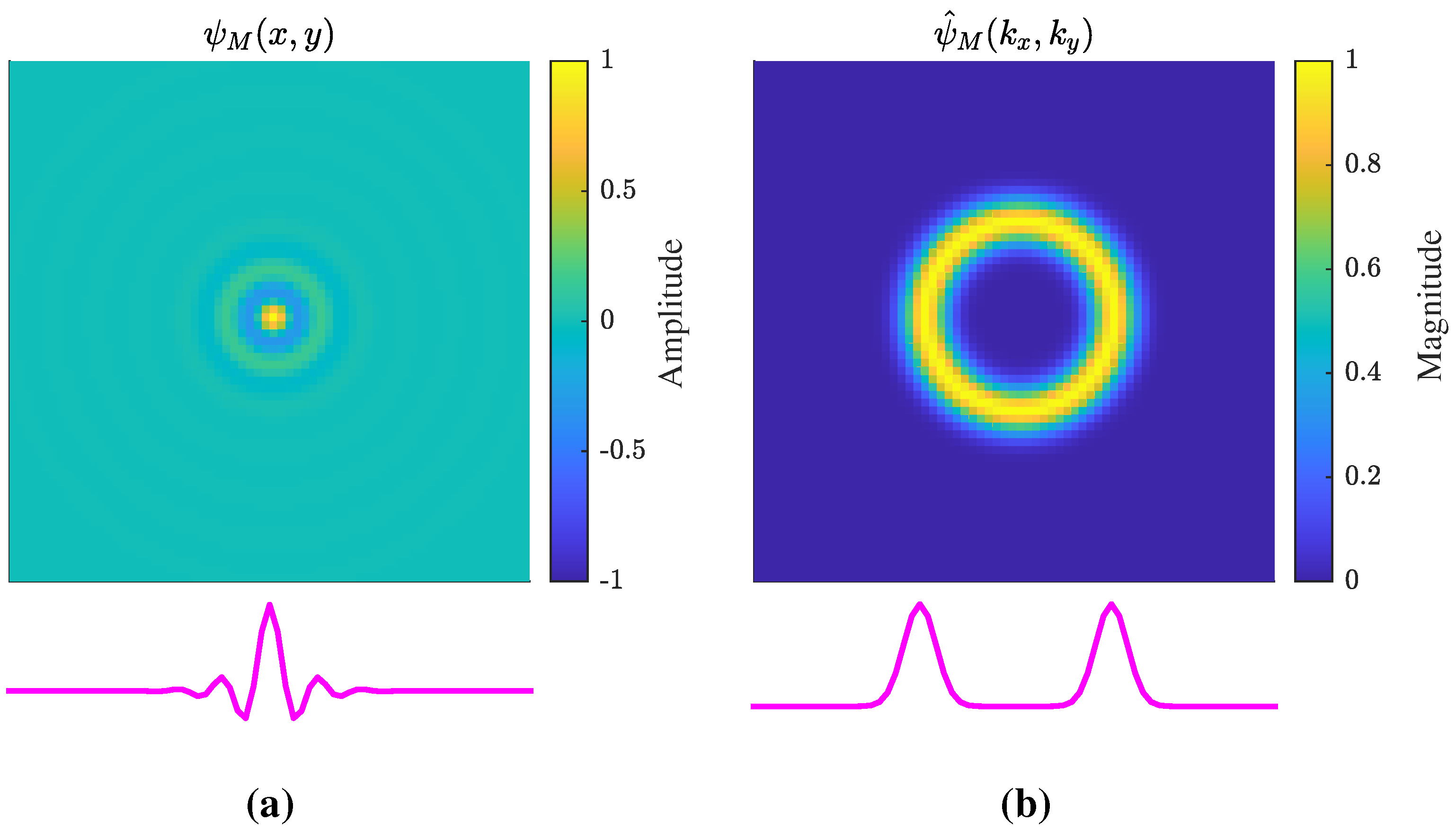
The Fourier transform of ${\psi }_M$, which is shown in space domain in Figure 10a, can be proven to be ${\widehat{\psi }}_M$ starting from the definition of directional Morlet wavelet with a spherical wave-vector [46], as represented in Figure 10b.

The continuous wavelet transform implemented is given by the:

$$C({\mathbf{x}}_{\mathbf{0}},a,f)=\sum _{\mathbf{x}}{U}_f(\mathbf{x},f){\displaystyle \frac{1}{a^2}}{\psi }_M\left({\displaystyle \frac{\mathbf{x}-{\mathbf{x}}_{\mathbf{0}}}{a}}\right)$$

(10)

where the scale parameter $a\ne 0$ is introduced. Equation (10) consists in computing the coefficient C of a series made of a 1D Fourier transform (in the time domain) and the 2D continuous wavelet transform (in the spatial domain). Smaller defects produce localized perturbations that are primarily observable at higher wavenumbers. To capture these features, the wavelet transform is $L1$-normalized [47]. This approach reduces the spectral overlap from larger scales (see Section 4.4), thereby increasing the sensitivity of the coefficients C at lower scale values a, where the effect of the defective region is expected to be greater. To compute C we need to select a properly value range for the parameter a and define the mother wavelet parameters ${\sigma }_0$ and $k_0$. The sufficient admissibility condition for the uniqueness of C has to be fulfilled: ${\widehat{\psi }}_M\left(\mathbf{0}\right)=0$, which implies $k_0\gg {\sigma }_0$. Antoine et al. [45] indicate ${\displaystyle \frac{k_0}{{\sigma }_0}}=6$ which guarantees it. To determine ${\sigma }_0$ and $k_0$, we can consider the central frequency of the wavelet $k_c$ and its support standard deviation ${\sigma }_c$ for a scale value a:

$$\begin{array}{c}{k}_c\left(a\right)={\displaystyle \frac{k_0}{a}}\hfill \\ {\sigma }_c\left(a\right)=a·{\sigma }_0\hfill \end{array}$$

(11)

The wavelet spectrum ${\widehat{\psi }}_M$ should be fully contained in the observable wavenumber range $(0,{\displaystyle \frac{2}{\Delta }})$, where $\Delta$ is defined in Table 1. Considering a central frequency array $k_c\left(a\right)\in \left(0,{\displaystyle \frac{2}{\Delta }}\right)$ uniformly sampled with the available spatial frequency resolution ${\displaystyle \frac{1}{(N-1)\Delta }}$ and hence the scale array a through Equation (11), the problem can be formulated as following (when the support $\widehat{\psi }$ is gaussian):

$$\begin{array}{cc}\hfill {\displaystyle \frac{k_0}{a_{\min }}}-3a_{\min }{\sigma }_0& >0\hfill \\ \hfill {\displaystyle \frac{k_0}{a_{\max }}}+3a_{\max }{\sigma }_0& <{\displaystyle \frac{2}{\Delta }}\hfill \\ \hfill {\displaystyle \frac{k_0}{{\sigma }_0}}& =6\hfill \end{array}$$

(12)

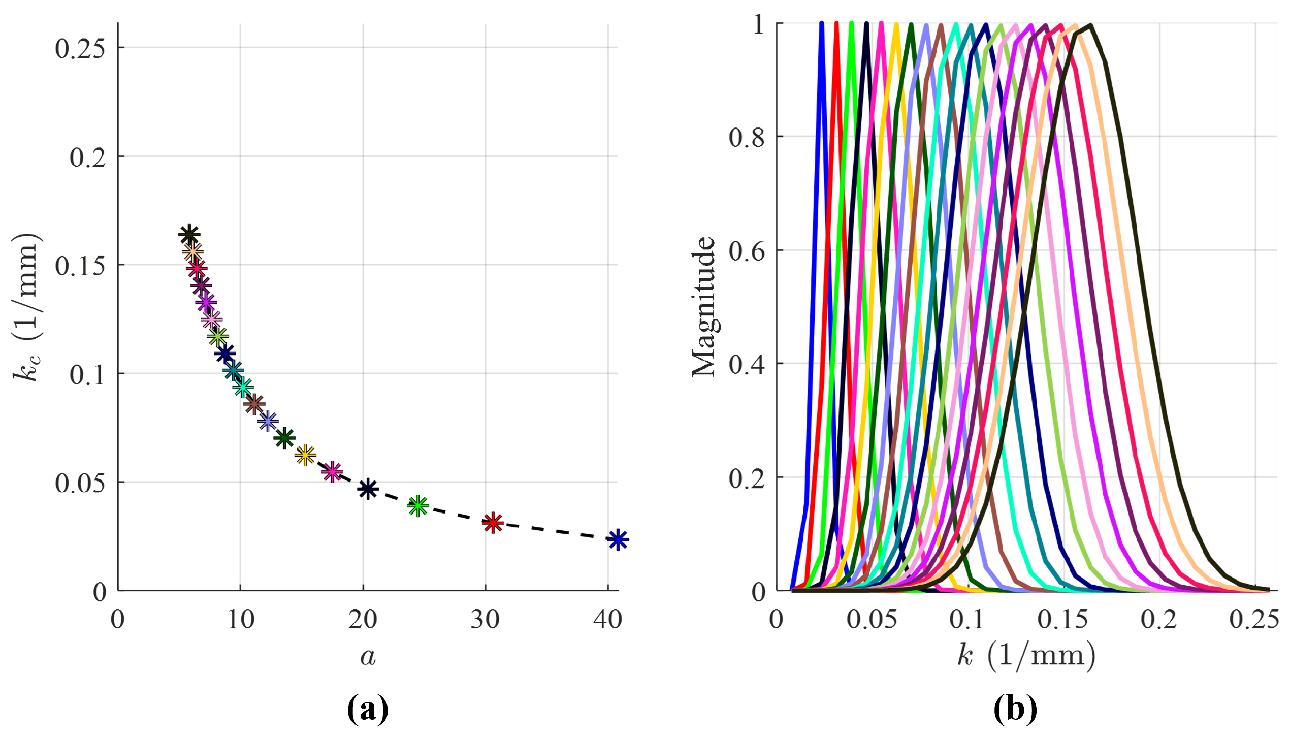
Fixing $k_0=6$, ${\sigma }_0=1$ an upper and lower bound for a can be calculated through Equation (12). The resulting filterbank through Equation (11) is shown in Figure 11. Each dot star included on the in Figure 11a represents the central frequency and the corresponding spatial scale value of the 2D isotropic Morlet wavelet while the magnitude spectrum for each wavelet is then represented by the curve of the same colour in Figure 11b.

The wavenumber imaging through 2D-CWT is explained according to the flowchart in Figure 9, analogous to the procedure used for the SSFT. The amplitude-compensated signal $u(x,y,t)$ is transformed into $U_f(x,y,f)$ via Fast Fourier Transform in time domain to extract spectral lines. In the acquired frequency band $F_b$, the spatial scale that maximize the wavelet transform coefficient at each spatial point and frequency line is calculated and then averaged into $\overline{a}$. In the spatial scale axis, the delamination, characterized by higher wavenumber values, appear at lower scale values with respect to the surrounding intact material for the Equation (11). To prevent inaccurate scale estimations at the boundaries of the acquisition region caused by truncated wavelets, a marginal border was excluded, following a rationale similar to the SSFT method. In this case it is determined considering the effective support of the background scale, corresponding strictly to half the size of the support ${\psi }_M\left({\displaystyle \frac{x}{\mathrm{mode}\left(\overline{a}\right)}}\right)$.

3.3. Entropy Based Threshold Binarization

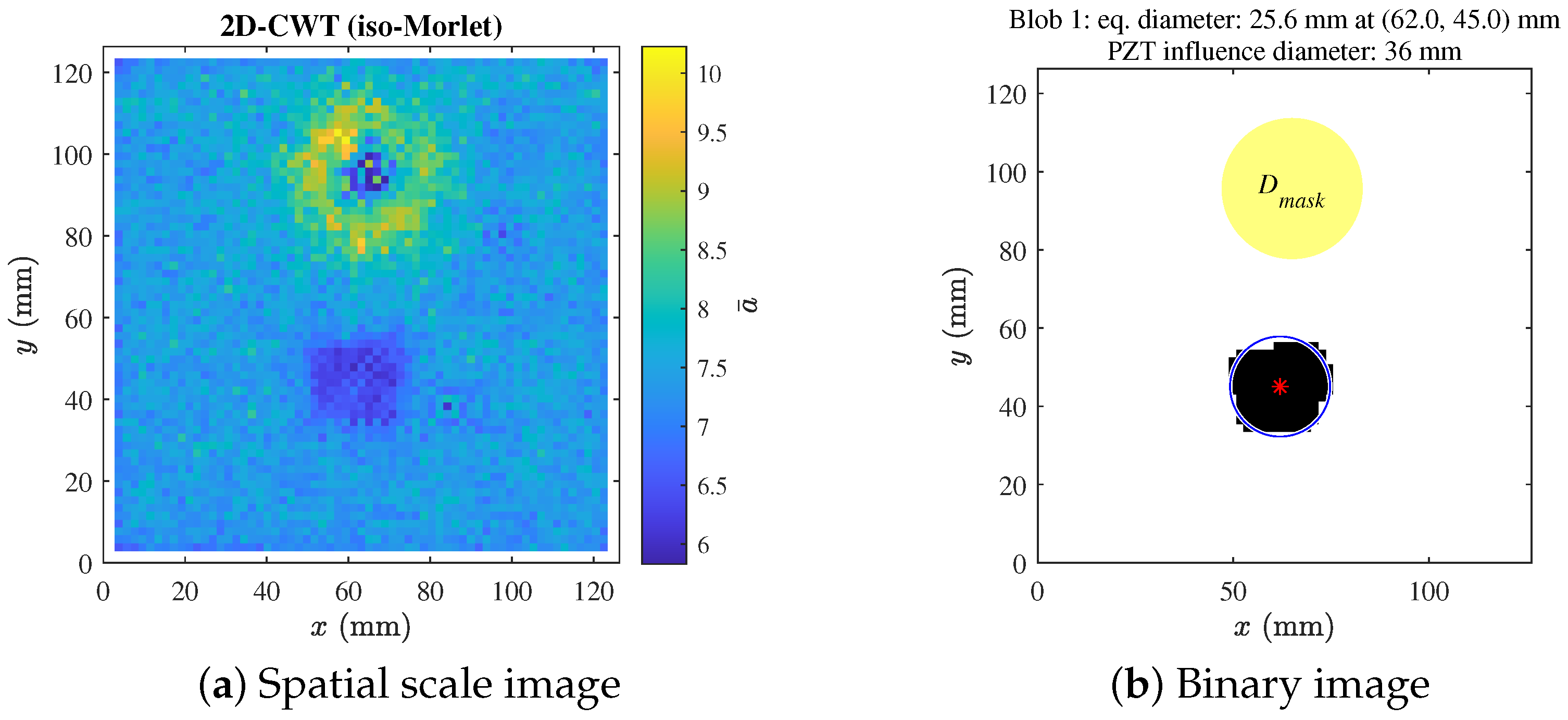
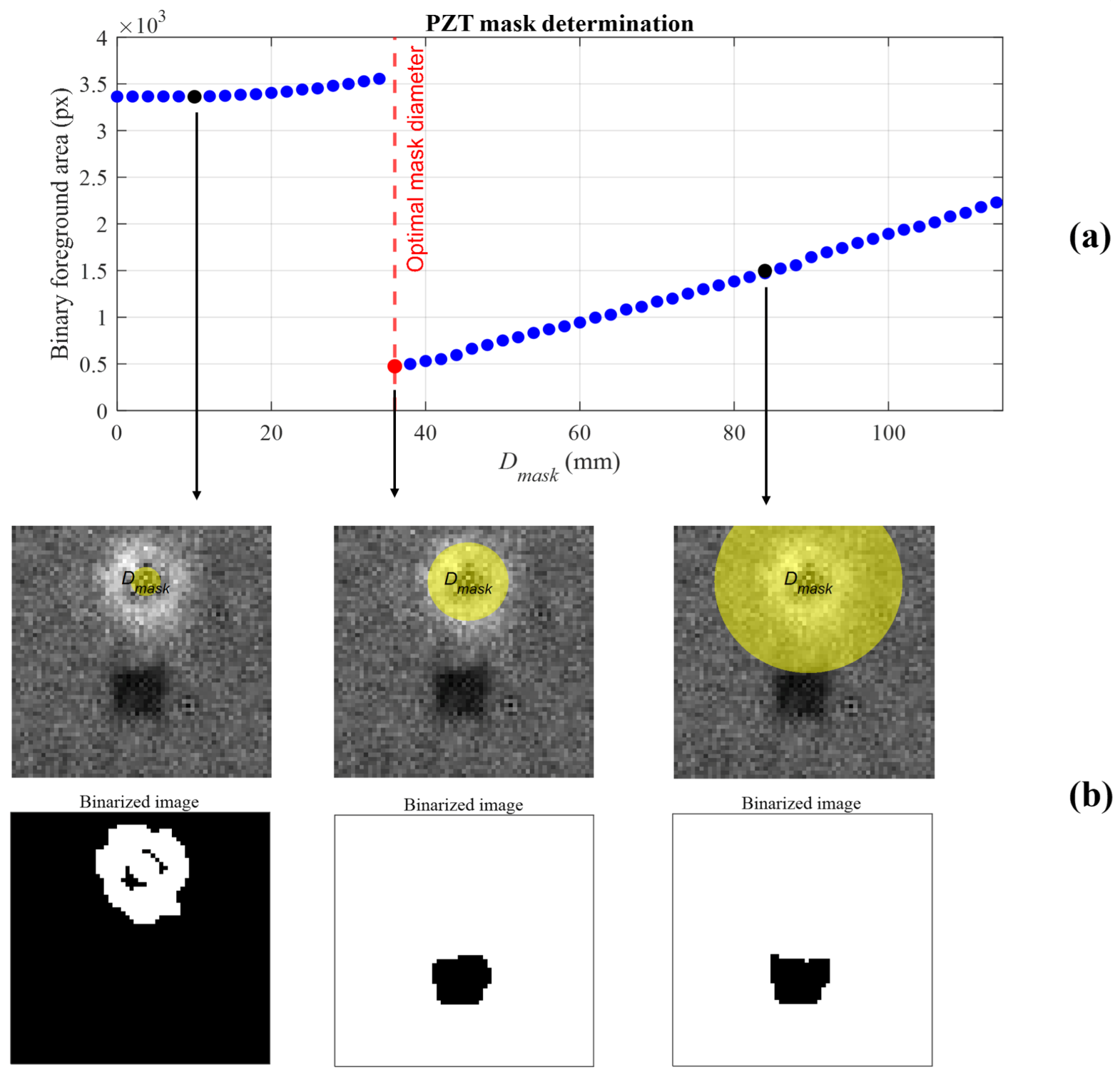
The final stage converts the continuous damage maps (from RMS, SSFT, or 2D-CWT) into a binary image to automatically identify and quantify the defect. To segment the defect from the background, we use an adaptive maximum entropy thresholding method based on the Kapur algorithm [48]. Specifically, the algorithm utilizes the image histogram to compute the independent Shannon entropies of the foreground and background classes for every candidate intensity threshold. The optimal threshold for binarizing the image is then selected as the value that maximizes the sum of these two entropies. An iterative step is necessary to neutralize the influence of the excitation source. In fact, the PZT disc generates high-amplitude near-field oscillations and adds thickness to the plate affecting Lamb waves dispersion curve. Therefore, this effect is not representative of the structural health status of the component. These related artifacts create a heavy tail in the image histogram, which distorts the statistical distribution and causes the maximum entropy thresholding to erroneously segment the source region as a defect. To prevent this, a circular exclusion mask is applied around the PZT centre, treating the enclosed pixels as Not-a-Number to exclude them from the entropy calculation. This approach ensures the comparison between investigated methodologies to be carried out excluding spurious components due to the excitation, which could lead to misinterpretations of the results. However, it must be noted that the exclusion mask introduces the inherent observability limitation: if an actual defect is located adjacent to the excitation zone, its localization can be prevented. The PZT influence diameter $D_{mask}$ is determined using a conditional stability criterion, operating under the assumption that the PZT disc interference is confined to an area smaller than the total scan region. To identify the optimal size, the algorithm iteratively tracks the binary foreground area and evaluates its derivative as the mask expands. During the evaluation, the PZT mask diameter is iterated over a range spanning from zero to the total width of the scan area. When an increase in the mask diameter causes a drop in the foreground area it indicates that the mask has successfully enveloped the PZT disc interference, allowing the exterior region to be correctly classified as the background. The optimal mask diameter is established at this precise point of area reduction. Conversely, if the area curve exhibits a continuously flat or immediately monotonic decreasing trend starting from a mask diameter of zero, it implies the absence of significant PZT interference, and the mask diameter is consequently defaulted to zero. The evaluation of the optimal PZT disc mask diameter is illustrated in Figure 12. In the upper graph, the binary foreground area in pixels is shown against the incremental diameter of the PZT mask. Three points in the plot (corresponding to a small, a large and the optimal mask diameter) are highlighted, reporting the PZT masks in yellow and the resulting binarized images in the row below.

The first plot of Figure 12a is characterized by a clear discontinuity. This occurs due to the PZT effect on the image. In fact, at low mask diameters, the histogram is dominated at high values by the PZT, causing the algorithm to misclassify the source itself as the foreground defect. In the case of a decreasing monotonic curve, a null diameter would be selected. Vice-versa, a sudden drop confirms that the high values associated with the source are finally covered; prior to this point, the algorithm was incorrectly considering the surrounding material as part of the defective region. With the interference masked, the exterior region is correctly classified as the background, and the optimal mask diameter is established at this precise point of area reduction. Once the mask is large enough to cover the PZT effects, the intensity distribution changes significantly; the algorithm correctly segments the actual structural damage in the surrounding material as the true foreground since it is represented by the lower tail values. The final step involves identifying and quantifying the isolated 0-filled regions (blobs) represented in black in Figure 12b. This is achieved using the standard CCL [49] algorithm implemented in Matlab version: 23.2 (R2023b) function ’regionprops’. In the 2D-CWT representation, lower average scales are associated with higher wavenumbers causing defective regions to exhibit lower scale values than the background. Consequently, the grayscale contrast is opposite to that obtained with the SSFT approach. For consistency in defect visualization and subsequent thresholding, the 2D-CWT image histogram is complemented so that defects are systematically displayed as black regions in both methods.

4. Results

In the following section we present the resulting images for all the considered defect detection methods with the indication of the blobs detected. With the exception of the first approach based on the simple RMS plot, the remaining compared methods share the common Lamb waves amplitude decay compensation pre-processing step highlighted in Figure 6. The fitted model D($\rho$) results with A = 0.019 ± 0.002 mm/s and $\lambda$ = 0.54 ± 0.04 for the regression curve confidence band $u_D$ at 95%. The fitted $\lambda$ results slightly higher than the theoretical 0.5 physically reflecting the additional composite-specific material attenuation. The coefficient of determination of the fit is $R^2$ = 90%. We deliberately opted for a simplified decay model in Equation (2). Near the finite-sized PZT actuator, complex wave interference occurs, making theoretical decay predictions impractical without highly specific models [39]. Thus, the fitted D curve serves as an equivalent decay model that conveniently lumps together near-field fluctuations, geometric spreading, and material attenuation. In this section, we firstly report a repeatability study in order to assess the quality and reliability of the experimental measurements. Secondly, we report the results of defect detection approaches relying on the RMS along time profile of the signals $v(x,y,t)$ and attenuation compensated ones $u(x,y,t)$. Next, we compare two different wavenumber imaging techniques: the standard SSFT based method and our proposed novel approach based on the 2D-CWT.

4.1. Repeatability Study

In the context of the proposed experimental framework, measurement repeatability has been strictly evaluated as a function of the spatial measurement point. In accordance with VIM, transposed by the standard UNI CEI 70099 [50], measurement repeatability is defined as the measurement precision evaluated under a set of constant repeatability conditions: experimental setup and measurement point(s) first. In the context of the presented experiment, for each scanning point a set of repeated 16 velocity signal acquisitions has been collected through the sLDV as shown in Figure 13. The inherent variability of the sLDV measurements in a scan point introduces a degree of uncertainty in the corresponding time averaged signal and, consequently, in the defect detection outcomes. The dispersion of the acquired velocity signal in a point is estimated through $L^2$ distance between the mean time profile. To systematically assess experimental repeatability, a point-wise statistical analysis of the repeated acquisitions has been performed. The variability of sLDV velocity signals was evaluated to characterize the repeatability of acquisitions in a representative scan point A. The repeatability test has been carried out through the Coefficient of Variance through norm $L^2$$\left(C{V}_{L^2}\right)$ to evaluate the dispersion of the acquired profile with respect to the RMS of the mean profile. The choice to refer to the RMS value of the average profile, instead of its mean, is due to the original CV definition which is not suited by the zero-mean vibration signal [51]. Instead, the following is implemented:

$$C{V}_{L^2}={\displaystyle \frac{\sqrt{\frac{1}{T}{\sum }_{t=1}^T{\left(\frac{S_{v\left(A\right)}}{\sqrt{K}}\right)}^2}}{\sqrt{\frac{1}{T}{\sum }_{t=1}^T{\left(\underset{k}{mean}\left(v\left(A\right)\right)\right)}^2}}}·100\%.$$

(13)

For a scan point A belonging to the grid, $C{V}_{L^2}$ is evaluated by varying the number of time averaging acquisition K among the available set for a maximum value of 16. At increasing K the $C{V}_{L^2}$ decreases as expected and for $K=16$ a $C{V}_{L^2}=21\%$ has been estimated as a result of the repeatability in this experimental case (Figure 14). In order to evaluate the uniformity of signal quality across the entire scanning grid, a spatial map of the $C{V}_{L^2}$ is plotted in Figure 15. It has been verified that the measurement precision is uniformly robust over the full domain, thus preventing spatial noise artifacts from being misidentified as structural defects during the subsequent damage detection phase. Spatial distribution of $C{V}_{L^2}$ presents the characteristic material anisotropic radiation pattern concentric to the PZT actuator. This trend indicates that the dispersion of the acquired signals at any given point depends on the local mean signal energy, which naturally decays as the Lamb waves propagate radially from the source. Once the acquired signals are compensated with a radial fitted attenuation curve, the measurement repeatability becomes spatially uniform. Downstream of this amplitude rescaling, the $C{V}_{L^2}$ is successfully constrained to a sufficiently low level (approximately $20\%$) within the region of interest encompassing the delamination, definitively confirming the reliability of the time-averaged data for the subsequent processing for defect detection.

4.2. Root-Mean-Square Based Defect Detection

The effect of wave amplification on the defective region can be observed in the RMS map calculated in time domain across the entire duration of the signal (Figure 16a). No automatic PZT masking is used to retrieve damage-related data with this method as the effect of the piezoelectric excitation appears spatially confined in Figure 16a.

By examining two points equidistant from the excitation source—point S in a sound region and point D over the delamination—a clear difference emerges. As shown in the top plot of Figure 16c, the signal amplitude at the defective position (D) is greater than the one corresponding to the intact position (S). This is also clearly confirmed broadband by observing the signal spectra (bottom plot of Figure 16d). It is worth noting that, due to the specific piezoelectric arrangement and the laser acquisition bandwidth, the fundamental anti-symmetric (A0) mode is detected as substantially predominant in the acquired wavefield (Figure 17). However, the binarized image related to the considered method (Figure 16b) exhibits a false-positive artifact resembling an anisotropic radiation pattern, demonstrating material anisotropy limits the detection accuracy. Furthermore, the identified region enclosing the delamination appears smaller than its actual dimensions.

4.3. Attenuation Compensated Root-Mean-Square Based Defect Detection

Compared to the original RMS velocity map shown in Figure 16a, the attenuation compensated RMS of $u(x,y,t)$ evidences higher contrast between the region affected by delamination and the intact remainder area (Figure 18a). Downstream the binarized process explained in Section 3.3 results in a false positive blob (Blob 1, Figure 18b). This has been caused by the wave reflections at the border of the panel that affect intensity distribution over the scan grid. Similarly to the previous method, no automatic PZT masking has been needed for this approach.

4.4. Wavenumber Imaging Based on SSFT Results

The following subsection presents the different results for the SSFT-based method, highlighting as the detection of the delaminated area depends on the window size parameter s. This can be seen in Figure 19. The average local wavenumber varies because the spatial frequency resolution increases as s increases. This affects image intensity histogram and related binarization process output. Increasing s implies a drawback: a larger margin of the original scanning area becomes inaccurate due to the truncation of the sliding spatial window. After the binarization process, the blob corresponding to the delamination remains visible for all tested values of s, but its size and location vary. Additionally, the material dispersion anisotropy causes false-positive blobs, in particular for lower values of s.

4.5. Wavenumber Imaging Based on 2D-CWT Results

The mean spatial scale assigned to each scan points throughout the 2D-CWT method is reported in Figure 20. The footprint of the PZT excitation is more clearly captured, requiring the masking algorithm to implement a non-zero diameter mask. The reason for this effect can be attributed to the use of progressively increasing scales within the wavelet filterbank (Figure 11), which results in a marked sensitivity to inherently broadband impulsive signals. In Figure 20a, the effect of anisotropic dispersion on the wavenumbers appears less evident; nevertheless, the defect is still correctly identified following the binarization process in Figure 20b.

4.6. Defect Detection Methods Comparison

The detection algorithm output for the various imaging methods are compared through the IoU [52]. By comparing the detected mask against the known ground-truth geometry of the defect, IoU is an indicator for detection accuracy. Results related to Figure 16b and Figure 18b–Figure 20b are reported in

Table 2. Defect detection algorithm comparison in terms of Intersection over Union scores and execution times.

Defect Detection Methods	IoU $\pm {\mathit{u}}_{\mathit{D}}$	Execution Time * (s)	Estimated Diameter (mm)
RMS	$10\%$	$48\pm 3$	13.1
Attenuation compensated RMS	$42\%\pm 3\%$	$105\pm 3$	15.7
SSFT (s = 5 mm)	$72\%\pm 0\%$	$169\pm 3$	18.6
SSFT (s = 10 mm)	$77\%\pm 0\%$	$175\pm 3$	20.7
SSFT (s = 25 mm)	$65\%\pm 1\%$	$174\pm 3$	26.9
SSFT (s = 50 mm)	$67\%\pm 1\%$	$176\pm 3$	25.5
2D-CWT	$66\%\pm 0\%$	$112\pm 3$	25.6

* mean ± 3 × standard deviation evaluated over 10 runs on DELL G7 7790 @2.60 GHz through Matlab script.

.

The SSFT method achieves the highest peak performance ($77\%$ IoU) with a specific window size $s=25$ mm and an estimated defect diameter $d_{estimated}=20.7$ mm, similar to the defect size. However, the 2D-CWT ranks similarly ($66\%$ IoU and an estimated defect diameter $d_{estimated}=25.6$ mm) while offering a significant operational advantage. The 2D-CWT does not require the selection of a window size, which is a parameter to which defect detection is shown to be sensitive by Table 2.

5. Conclusions

The application of a wavenumber imaging technique proves to be a more accurate methodology for non-destructive evaluation of composite panels defects compared to a simple RMS metrics in the case of LDV measurement. The 2D-CWT overcomes the primary limitation of the dependency on a fixed spatial window size with respect to the standard LWE technique based on SSFT. Experimental results demonstrate that SSFT, which is sensitive to window size selection, can achieve high detection accuracy (up to $77\%$ IoU) for a particular parameter but performance drops to $65\%$ when the window size is suboptimal. The 2D-CWT eliminates this trade-off by allowing the analysis to signal features using the scale parameter as a pseudo-wavenumber, thereby removing the need for a priori knowledge of defect dimensions. Furthermore, the integration of adaptive maximum entropy thresholding and a piezoelectric source exclusion masking successfully isolates structural damage from the surrounding intact material. Consequently, the 2D-CWT method represents an operational advancement for LWE methods, offering a flexible, automated, and baseline-free solution for quantitative damage assessment in composite panels.The proposed 2D-CWT method ranks 66% IoU, but with a lower computation time (112 ms $\mathit{vs}$ max. 176 ms for SSFT in the used machine). A fundamental limitation of the current static 2D-CWT approach lies in the inherent spectral bandwidth of the wavelet at any given scale. Consequently, multiple propagation modes may coexist and overlap, potentially altering the damage signature in a different defects scenario. As discussed in Section 4, an additional uncertainty on the defect detection stems from dispersion anisotropy observed. We acknowledge how to effectively integrate the information regarding dispersion anisotropy into the defect detection framework pre-processing remains a subject for a future work. Results obtained in the present work are summarized in the following:

• The spatial window size characterizing SSFT is not a relevant parameter in case of 2D-CWT (spatial resolution remains unchanged).
• The 66% IoU remains constant despite the uncertainty of the attenuation model.
• 2D-CWT gets a lower execution time with respect to SSFT.
• The proposed algorithm is unsupervised.

Moreover, the following main limitation characterize the study:

• The tested panel material anisotropy should be mild. Since the maximum entropy thresholding relies on the statistical separability between intact and damaged wavenumber distributions, severe anisotropy could diminish this separation due to anisotropic pattern of the background wavenumbers. To extend the proposed framework to highly anisotropic structures, a pre-filtering step (e.g., applying a radial pattern filter as done in [37]) before binarization processing would be required to mitigate this anisotropic effect.
• Surface roughness has been assumed constant (e.g., assuming no wear caused by concentrated loads).
• Assessment only of a single type of defect.
• Presence of a singular excited mode A0.