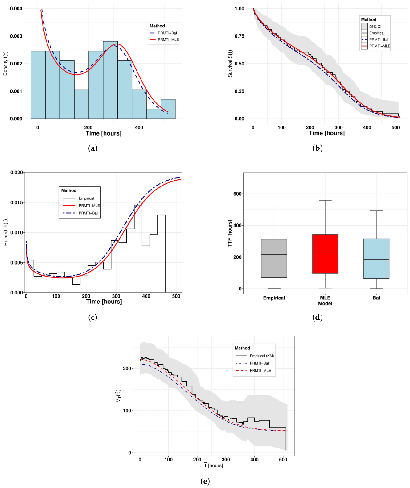
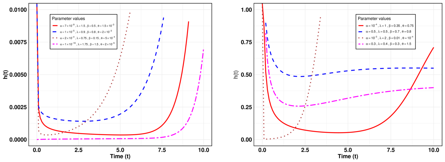
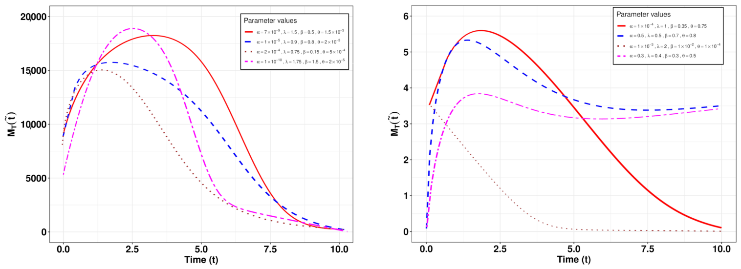
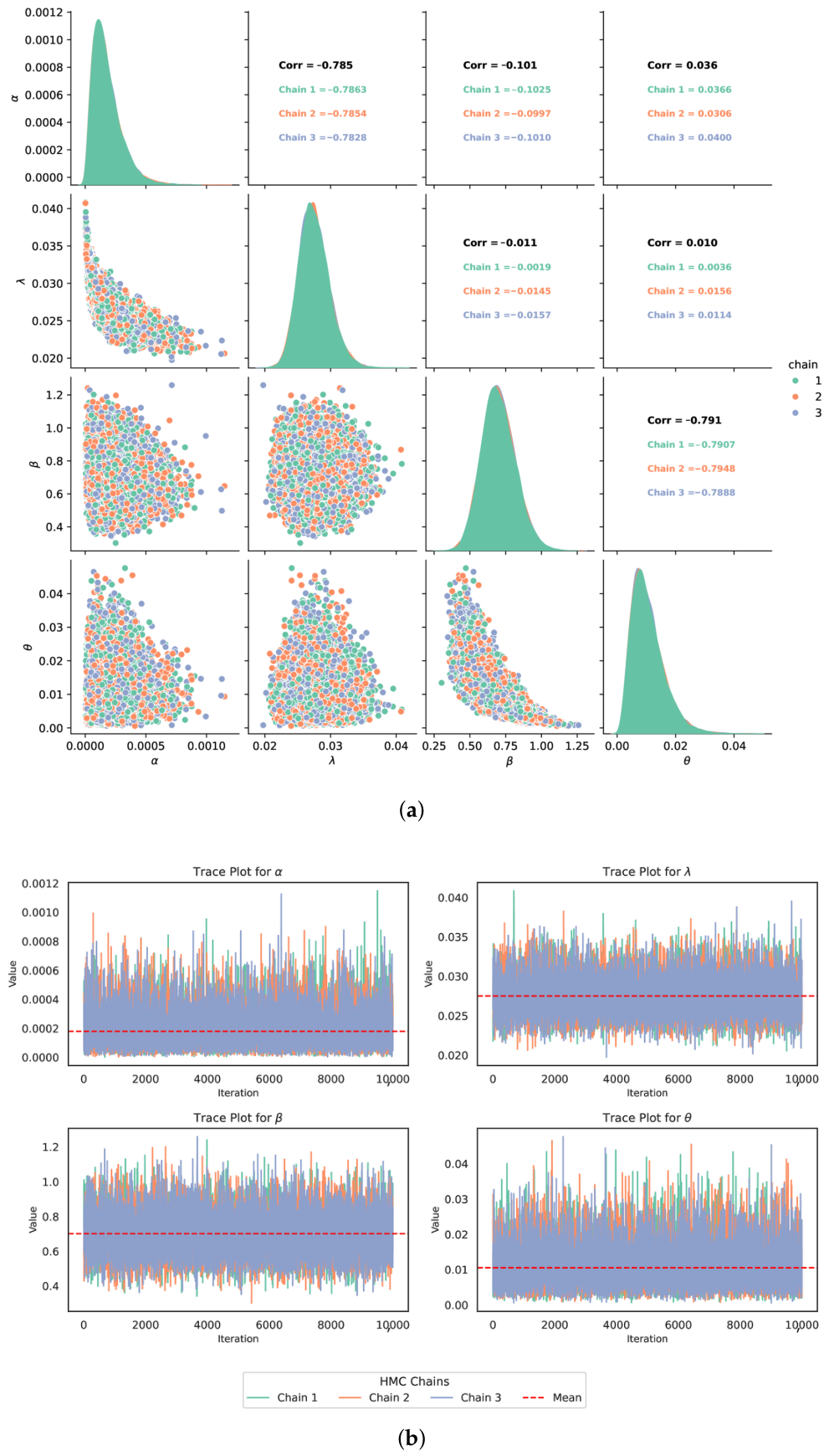
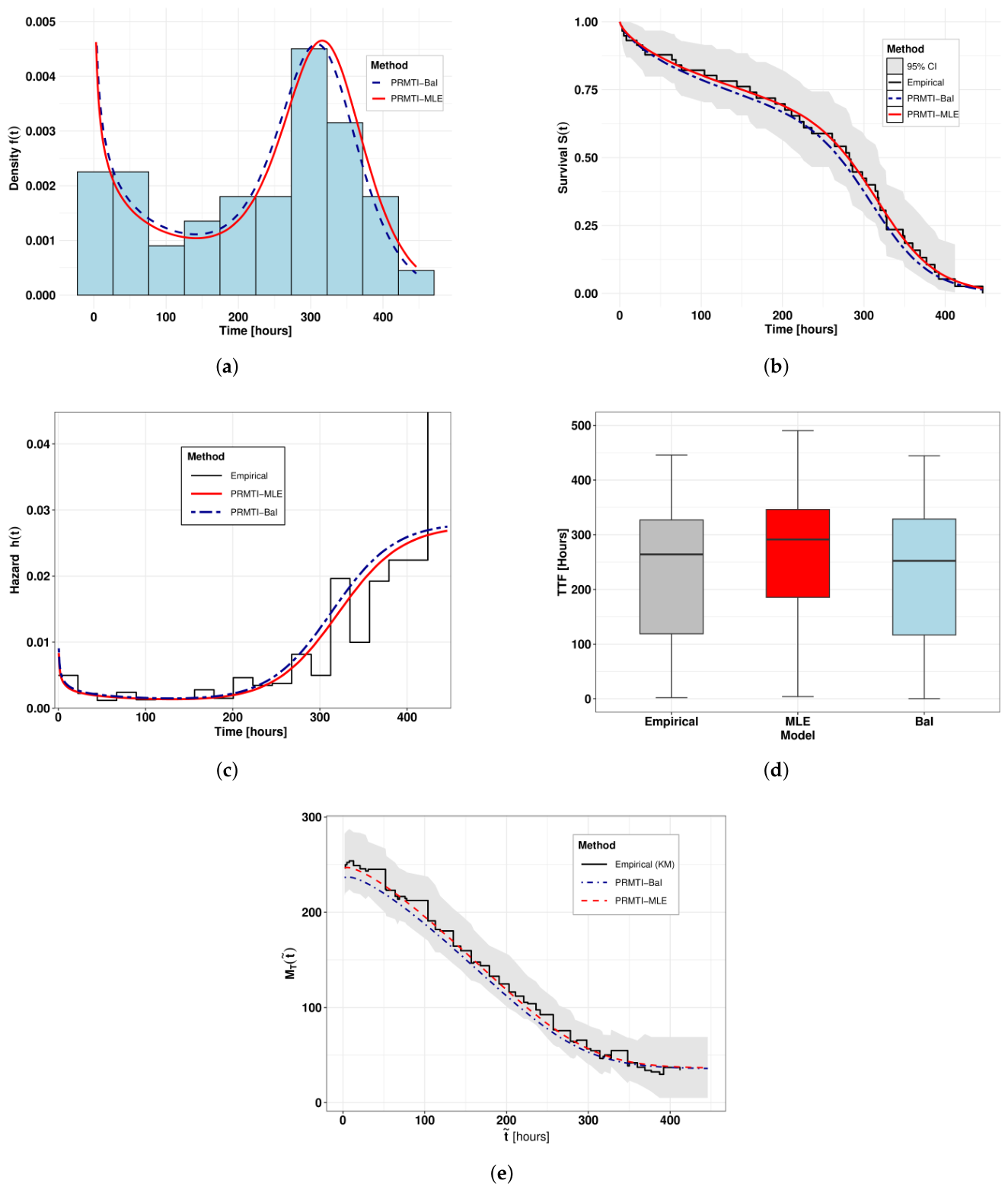
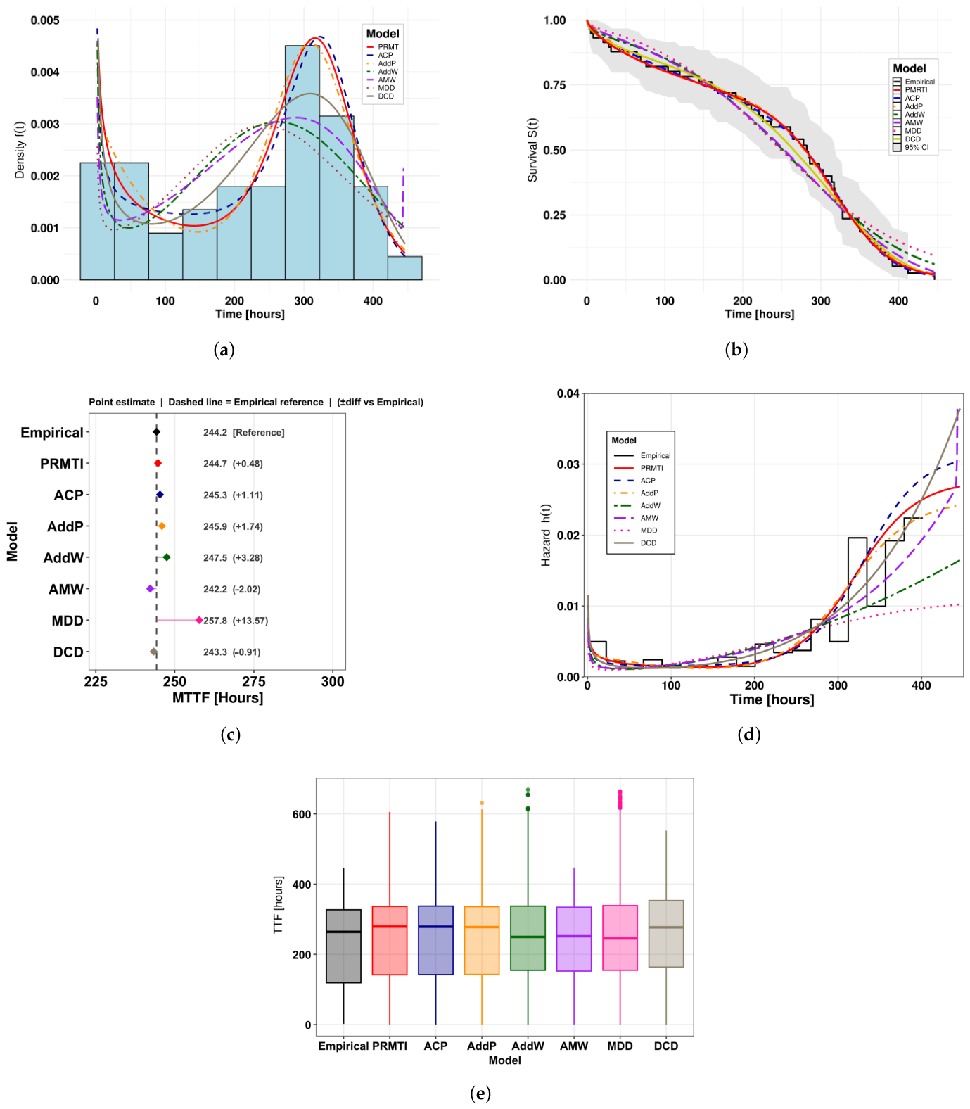
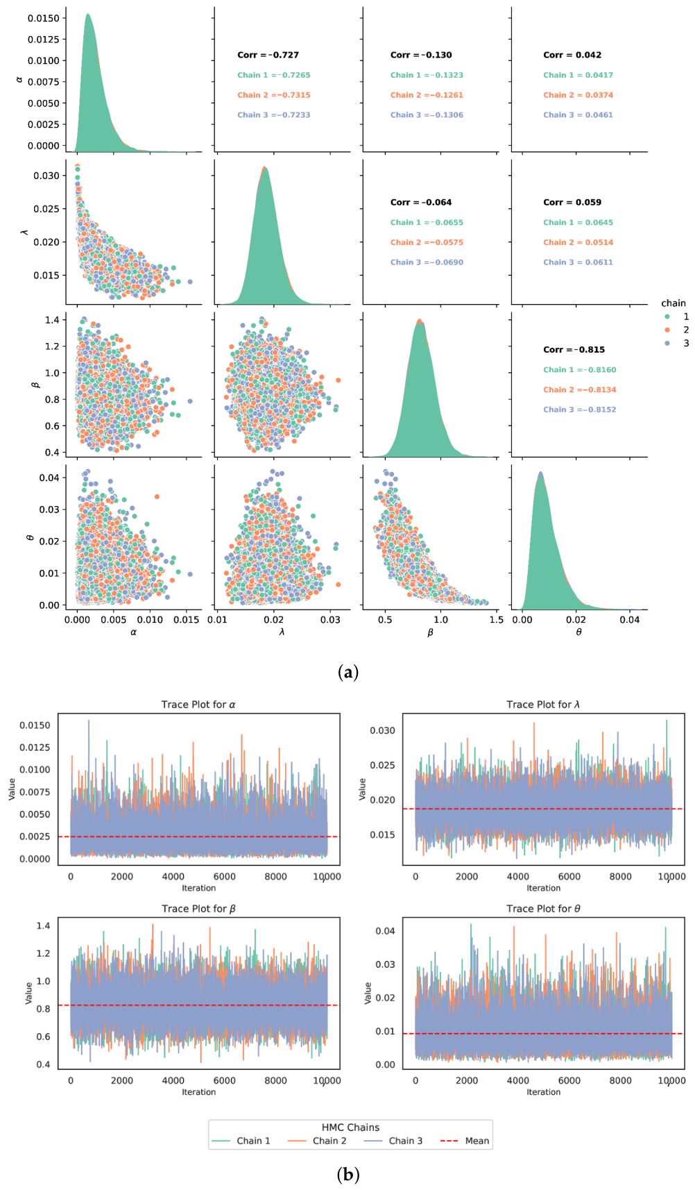
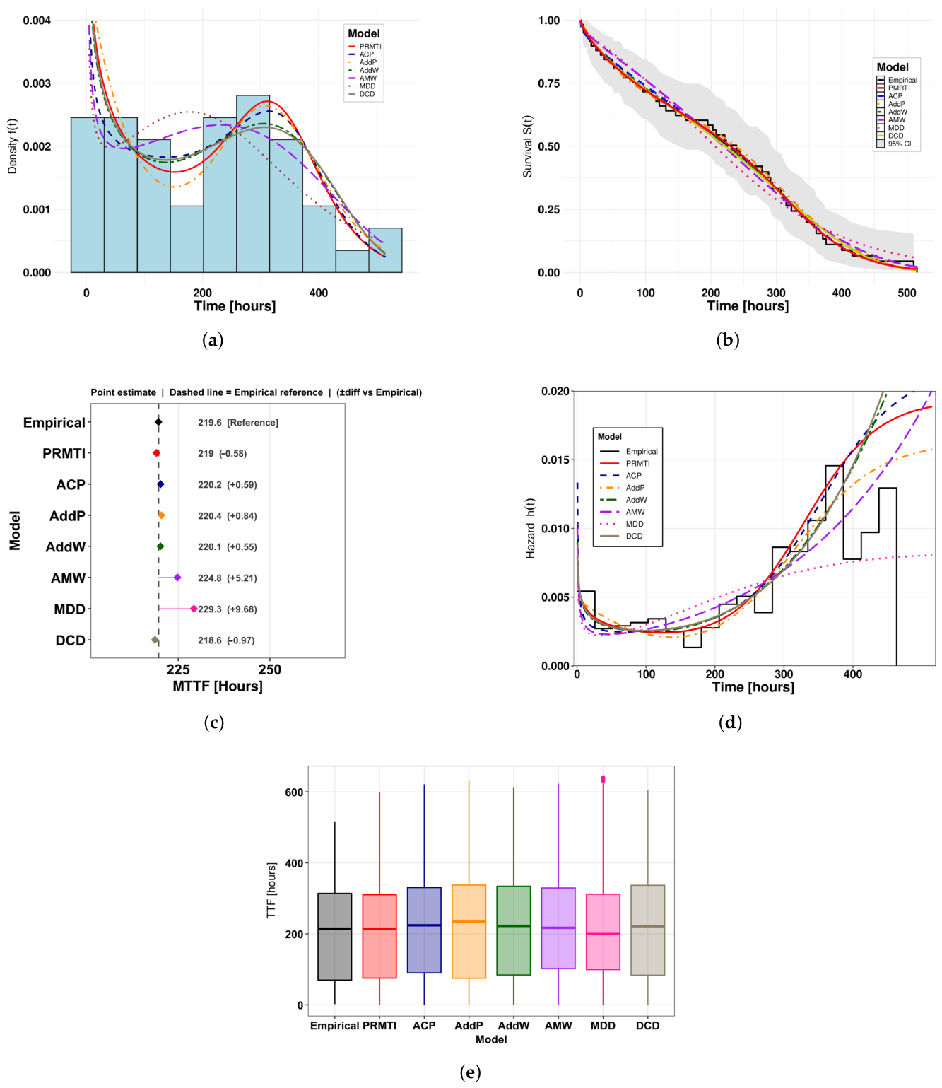
Flexible Reliability Assessment of Electronic Components Under Complex Failure-Mode Scenarios

Abstract

One of the most important aspects of reliability engineering is modeling the failure behavior of devices, which can exhibit monotonic or non-monotonic patterns and depend explicitly on design, internal components, and operating conditions, often leading to multiple failure modes. Methodologies exist to address these scenarios; however, many lack the flexibility to capture diverse behaviors throughout the device’s lifespan. Given this, this paper presents a novel reliability model based on the Competitive Risk (CR) framework. This model comprises a minimal variable derived from the Perks Risk Model Type I (PRMTI) to capture risk-rate patterns of different shapes. Unlike existing CR and additive models, the proposed approach effectively handles failure-time data with increasing, bathtub, inverted, or modified risk rates. Relevant mathematical properties for reliability scenarios are presented and analyzed. Furthermore, two approaches for parameter estimation are offered: the maximum likelihood method (MLE) and Bayesian inference (BaI) using the Hamiltonian Monte Carlo (HMC) method. Finally, to verify the proposed methodology, two case studies and a comparative analysis are presented, in which the PRMTI is tested against six other methodologies with similar properties. The results show that the PRMTI outperforms empirical calculations, offering greater agreement and more accurate predictions of failure probabilities. These findings highlight the model’s versatility and accuracy in representing complex failure mechanisms in reliability studies.

1. Introduction

Reliability analysis is a tool used in the manufacturing sector to describe the behavior of electrical, electronic, and mechatronic devices; however, this analysis is becoming increasingly complex in both practice and theory. This complexity stems from the growing use of semiconductor devices and flexible hybrid electronics in modern device designs, which substantially alter failure patterns throughout the product’s lifespan. From a reliability perspective, the Hazard Rate Function (HRF) is key to understanding a product’s evolution throughout its operational life, and this evolution is expressed by the Bathtub Hazard Rate (BHR). The BHR defines the three phases a product experiences over time: infant mortality, where early failures can be detected and warranty policies are defined; normal operating life, where the device operates stably without critical or catastrophic failures; and, finally, wear and tear, where the probability of failure within the device increases and where it is advisable to implement preventive maintenance policies to prolong the useful life of the product.

Recent research has demonstrated the need for analytical and practical advances in reliability models that more accurately represent the behavior of devices experiencing both monotonic and non-monotonic failures. In this regard, Bakouch et al. [1], Du and Sun [2], Gaonkar et al. [3], Al-Essa et al. [4], Hromádka and Martínek [5], He et al. [6], and Zheng and Su [7] have established that the flexibility of reliability models is essential for accurately assessing equipment behavior under real operating conditions, not only in the laboratory. Furthermore, these studies agree that poor product performance estimates can lead to inadequate warranty policies, maintenance strategies with little impact on the product, and a significant decrease in consumer confidence in manufacturers. Consequently, reliability analyses must keep pace with the development of new technologies, which implies that classic reliability distributions and models, such as exponential, Weibull, and lognormal models, may be limited in their ability to capture a device’s failure patterns.

Based on the above, various models have been developed to flexibly represent the HRF. Lai et al. [8] proposed the modified Weibull Additive Distribution (AWD), which characterizes the distribution of extreme Weibull Type I values. Xie et al. [9] extended the analysis by introducing a shape parameter, thereby allowing for the capture of both regular and irregular shapes, including monotonic and non-monotonic behaviors. A variable-scale parameter was introduced to link uncertainty to variations in the device’s failure interval. Other contributions along the same lines can be found in [10,11]. However, the aforementioned works have practical limitations: they depend heavily on the quality and quantity of data collected during experiments, which limits the accuracy of parameter estimates and leads to underfitting in the device representation relative to empirical behavior.

Another methodological approach is the Alpha Transformation, introduced by Mahdavi and Kundu [12] and Mead et al. [13], which adds a parameter to base distributions to control skewness and represent non-monotonic behavior. Meanwhile, Kumar et al. [14], Deepthi and Chacko [15], and Maurya et al. [16] proposed the DUS transformation, which exponentiates the Cumulative Distribution Function (CDF) to enable more flexible models with computational savings in parameter estimation. Other relevant transformations include those of Shama et al. [17], Pararai et al. [18], and Ahsan-ul Haq et al. [19]. However, these methodologies have limitations: reduced flexibility in identifying phase shifts in the HRF, sensitivity to extreme values, and poor fits to the tails of the distribution.

Xie and Lai [20] proposed the Additive Weibull Distribution (AWD), which combines two Weibull HRFs to form a four-parameter model that captures non-monotonic and BHR behaviors, surpassing the base Weibull model. Thanh Thach and Briš [21] proposed a model that adds the Chen and Weibull distributions, thereby improving accuracy in estimating the device’s lifetime behavior; however, the limitations of the Chen distribution constrain the identification of BHR transition points. Abd EL-Baset and Ghazal [22] proposed a five-parameter model by generalizing the AWD, allowing for greater flexibility in representing the HRF; however, given the model’s complexity, its practical application is limited by computational cost and the high risk of overestimating failure times, leading to non-universal generalization. The models do not consider multiple failure modes in their applications, thereby limiting their applicability to real-world scenarios.

Given the methodological limitations of state-of-the-art research on the capture of the behavior of systems with complex failures, there is a need to explore alternative approaches to reliability analysis. In this regard, competitive risk (CR) models are well suited to establishing a framework in such cases, as they enable analysis of scenarios in which a failure may be attributable to multiple potential causes. This prevents the elapsed time since the event of interest from being influenced by other risk sources that could mask its occurrence, thereby enabling a more realistic representation of the device’s reliability.

Building on this framework, Fan et al. [23] studied k failure modes with lifetimes following a joint k-variate Marshall–Olkin Weibull distribution under multiple censoring, focusing on communication transmitters. The authors note that MLE requires additional constraints when the shape parameters are unequal due to the distribution’s structure. In a similar line of research, Dutta et al. [24], Abba et al. [25], Ranjan and Upadhyay [26], Singh [27], and Al-Essa et al. [28] proposed CR models under the assumption that failure causes behave in a constant or monotonic manner over time. However, empirical data (see [29,30]) challenge this assumption, revealing that at least one failure mode may exhibit a non-monotonic pattern. Furthermore, the models are based on variants of classic distributions, overlooking the HRF associated with the cause of individual failure, which can introduce bias when estimating product life and calculating failure probabilities in the presence of censored devices in the experimental data.

The methodological framework of CR models supports the development of hybrid models that incorporate HRFs from various scientific fields for reliability analysis. Several studies, including those by Méndez-González et al. [31], Zeng et al. [32], and others, have shown that the Perks distribution, originally used in actuarial mortality research, can be effectively applied to engineering reliability modeling. This adaptation exploits the similarity between biological survival curves and the BHR patterns observed in reliability, providing a more relevant representation than traditional models. It captures moderate aging effects without excessive risk acceleration. By accurately representing the three BHR phases, this distribution aids in the optimization of preventive maintenance, such as by precisely identifying wear points for the scheduling of replacements. Ultimately, the Perks distribution models failures caused by cumulative wear from gradual internal component degradation, featuring a period of stable operation before increased failure risk due to damage accumulation.

In another vein, the Risk Model Type I (RMTI) proposed in [33] is considered an alternative to the classic Weibull, exponential, and extreme value distributions because it allows for a more robust fit and representation. This makes it suitable for modeling of the behavior of more complex devices where a single failure mode (FaM) does not predominate, thereby more accurately reflecting real-world behavior. This characteristic of the RMTI allows for a risk calculation structure that is more sensitive to early changes, that is, it captures failures with a high initial rate of variation or latent defects. This means that equipment failures can be attributed to manufacturing defects or assembly errors, with an initial failure probability that increases, then decreases as the weakest components fail prematurely.

Along the same lines, Iliyasu et al. [34] proposed a modified Dhillon distribution (MDD) based on the Beta function. While the MDD fits well compared to other similar models, the survival function is constrained by the Beta distribution’s domain, which prevents characterization of the device’s performance throughout its entire operational phase. To address these limitations, Amiru et al. [35] introduced the Dhillon–Chen Additive Distribution (DCD); however, because the Chen distribution is skewed, it introduces significant bias when fitting device lifetimes.

Despite their potential, the Perks and RMTI models have not been thoroughly explored in reliability analysis. This is primarily because (i) these models do not traditionally originate from the domain of reliability practitioners and (ii) there is a methodological challenge in modeling multiple FaMs that compete for dominance in the device. To address these gaps, this paper proposes a four-parameter Perks–RMTI hybrid model (PRMTI) that captures dependencies between dual FaMs in devices within a unified analytical framework. Notably, the RMTI and Perks models differ qualitatively and structurally from previous proposals, such as those mentioned in [36,37]. While traditional approaches tend to impose rigid geometric constraints—whether polynomial or double-exponential—on the initial lifetime of a device, the proposed model breaks this rigidity by offering high asymptotic flexibility at the beginning of the device’s life cycle. This is achieved through the dynamic adaptation of the infant mortality curve, which is governed by the shape parameters. Thus, the risk at startup ($t=0$) can be a fixed positive value or a rate that tends toward infinity. This characteristic is vital in reliability practice, as it allows for the modeling of minor initial failures or extremely aggressive degradation processes in the early stages of operation with the same mathematical rigor, without complicating the overall analytical framework.

Complementarily, the mathematical properties discussed here enable a clearer separation of the origins of defects in a part. On the one hand, manufacturing defects manifest as the device’s infant mortality and can be identified using RMTI elements. On the other hand, aging effects resulting from accumulated wear are captured by the Perks distribution. This separation prevents the mixing of failure causes of different natures, ensuring that parameter correlations remain within their respective components and do not distort the overall model. The result is a significant reduction in parameter confusion and the weak identifiability problems that often complicate frameworks such as AddP or ACP.

The proposed methodology can be applied in reliability engineering by providing a framework for the linking of parameters to failure patterns and offering a more reliable representation of BHR behavior. This enables device manufacturers to draw inferences for diagnosis and decision-making grounded in reliability engineering principles. The reliability indicators derived from the proposed model, such as HRF, Mean Time to Failure (MTTF), and Mean Residual Lifetime (MRL), are key tools that can be directly integrated into maintenance optimization frameworks. Recent literature strongly supports this approach from multiple perspectives. For example, in systems with competing failure modes, Duan et al. [38] developed a two-level maintenance model that optimizes costs and availability based on remaining useful life. In contrast, Gan et al. [39] demonstrated that such scenarios require highly flexible models capable of capturing non-monotonic behavior. On the other hand, accuracy in risk modeling is crucial for establishing optimal thresholds, as evidenced by the condition-based maintenance policies proposed by Luo et al. [40]. Finally, inspection strategies have been made more sophisticated by incorporating state beliefs into the Semi-Markov Decision Process [41] and by multilevel inspection schemes for systems with protection components [42], where characterizing fault-propagation mechanisms is essential. Taken together, these studies demonstrate that the scope of the PRMTI model extends beyond simple statistical fitting, establishing it as an operational decision-making engine for the manufacture of electronic devices.

The specific objectives of this paper focus on the following aspects:

(i)

We present an alternative two-failure-mode CR model that addresses the limitations of earlier models by combining monotonic and BHR behaviors.

(ii)

We explore and analyze risk functions from disciplines outside of reliability to integrate them into CR models for a more flexible and realistic representation of device lifespan.

(iii)

We outline and discuss the characteristics of the PRMTI for device lifetime analysis, targeting reliability practitioners.

(iv)

We present two estimation approaches for PRMTI parameters: one based on MLE and the other using BaI via the HMC algorithm.

(v)

We evaluate the performance and applicability of the PRMTI model against recent CR-based methodologies and models representing monotone and non-monotone behaviors using diverse, representative datasets.

Finally, this paper is structured as follows: Section 2 introduces the PRMTI model and outlines the various forms of the HRF. Section 3 details key mathematical properties for reliability analysis. Section 4 outlines inference methods using MLE and BaI via the HMC algorithm to estimate the parameters of the proposed model. A simulation study is conducted in Section 5 to assess the performance of the proposed MLE and BaI methods for PRMTI. Section 6 presents case studies and analyzes the results from each dataset. Finally, Section 7 concludes with the findings and potential directions for future research.

2. Preliminary Notation and PRMTI Model Description

We begin by scoping the CR model formulation with the following assumption: consider a set of $\mathbb{P}$ parts that are identical in their manufacturing configuration and operate independently of one another. Each component can fail due to one of $\omega$ independent FaMs, where $\omega \ge 2$, each attributed to a single cause. The experiment concludes when all devices have failed or the maximum censoring time is reached. For every component that fails during the test, we record two pieces of information: the failure time of the device, denoted as T, and the cause of failure, represented by $\zeta$, where $\zeta ϵ(1,2,\cdots \omega )$. In scenarios involving censoring, the only measurable quantity is the censored time, which we denote as $\zeta =0$.

2.1. Preliminary Notation

Based on the given information, the key functions for reliability analysis, represented by $f_{\mho }\left(t\right)$, $S_{\mho }\left(t\right)$, and $h_{\mho }\left(t\right)$, correspond to the Probability Density Function (PDF), the Reliability Function (RF), and the HRF for the distribution of $T,\zeta \in (1,2,\dots ,\omega )$ under the CR methodology. These are expressed as follows:

The RF of $S_T\left(t\right)$ is expressed as

$$S_T\left(t\right)=Pr(T_1>t,T_2\cdots \omega )={\displaystyle \prod _{\mho =1}^{\omega }}{S}_{\mho }\left(t\right)=exp\left[-{\displaystyle \sum _{\mho =1}^{\omega }}{\int }_0^t{h}_{\mho }\left(u\right)du\right].$$

(1)

The PDF $f_T\left(t\right)$ is given by

$$f_T\left(t\right)={\displaystyle \sum _{\mho =1}^{\omega }}{f}_{\mho }\left(t\right){\displaystyle \prod _{\rho =1,\rho \ne \mho }^{\omega }}{S}_{\rho }\left(t\right)={\displaystyle \sum _{\mho =1}^{\omega }}{h}_{\mho }\left(t\right){\displaystyle \prod _{\rho =1}^{\omega }}{S}_{\rho }\left(t\right)$$

(2)

Finally, the HRF $h_T\left(t\right)$ can be represented as:

$$h_T\left(t\right)=h_1\left(t\right)+h_2\left(t\right)+\cdots +h_{\omega }\left(t\right)={\displaystyle \sum _{\mho =1}^{\omega }}{h}_{\mho }\left(t\right),$$

(3)

where $h_{\mho }\left(t\right)$ represents a particular mode of the HRF associated with the ${\mho }^{th}$ risk or cause, defined as follows:

$$h_{\mho }\left(t\right)=\underset{\Delta t\to 0}{lim}{\displaystyle \frac{Pr\left(Y<t+\Delta t,\omega =\mho |T\ge t\right)}{\Delta t}}$$

2.2. PRMTI Model Description

For the PRMTI model proposed in this paper, it is necessary to define the two failure time models; for this, we establish the following.

Let T be a random variable for the Perks distribution; therefore, the PDF of T is defined as follows:

$$f_1\left(t\right)=\alpha \lambda e^{\lambda t}{\displaystyle \frac{\left(1+\alpha \right)}{{\left(1+\alpha e^{\lambda t}\right)}^2}},t>0$$

(4)

where $\alpha ,\lambda >0$ and represent the shape and scale parameters, respectively.

In turn, let us consider that, for a random variable (T), the PDF of the RMTI distribution is represented by

$$f_2\left(t\right)={\displaystyle \frac{\beta \theta t^{\beta -1}}{{(\theta t^{\beta }+1)}^2}},t>0,$$

(5)

where $\beta ,\theta >0$, representing the shape and scale parameters, respectively.

Given the above, let us start by stating that we perform a reliability analysis with P components or devices that are identically manufactured, and their operation is independent. In turn, the parts under analysis have only two FaMs, that is, $\omega =2$, which we will classify as FaM1 and FaM2. Also, let $T_{𝚤,1}$ and $T_{𝚤,2}$ represent subject ${𝚤}^{\prime }s$ failure times from FaM1 and FaM2, respectively, with these failure times ranging in the order of $𝚤=1,2\cdots \omega$, where $T_{𝚤,1}\sim Perks(\alpha ,\lambda )$ and $T_{𝚤,2}\sim RMTI(\beta ,\theta )$, so that it is assumed that the model is described by two different models with non-monotonic and monotonic properties. Then, the $S\left(t\right)$ and $h\left(t\right)$ for each failure mode are defined as follows:

For FaM1, based on (4):

$$S_1\left(t\right)={\displaystyle \frac{\left(1+\alpha \right)}{\left(1+\alpha e^{\lambda t}\right)}},h_1\left(t\right)={\displaystyle \frac{\alpha \lambda e^{\lambda t}}{1+\alpha e^{\lambda t}}}$$

For FaM2, based on (5):

$$S_2\left(t\right)={(\theta t^{\beta }+1)}^{-1},h_2\left(t\right)={\displaystyle \frac{\beta \theta t^{\beta -1}}{\theta t^{\beta }+1}}$$

The TTF, represented by $T_{𝚤}$, is defined as the minimum of $T_{𝚤,1}$ and $T_{𝚤,2}$, i.e., $T_{𝚤}=min(T_{𝚤,1},T_{𝚤,2})$. Assuming that $T_{𝚤,1}\sim Perks$ and $T_{𝚤,2}\sim RMTI$ and following (2), we can express the PDF as follows:

$$f(t,\varphi )=\left[{\displaystyle \frac{\alpha \lambda e^{\lambda t}}{1+\alpha e^{\lambda t}}}+{\displaystyle \frac{\beta \theta t^{\beta -1}}{\theta t^{\beta }+1}}\right]·{\displaystyle \frac{\alpha +1}{\left(1+\alpha e^{\lambda t}\right)\left(\theta t^{\beta }+1\right)}},t>0,$$

(6)

where $\varphi ={(\alpha ,\lambda ,\beta ,\theta )}^{\prime }$ represents the vector of the PRMTI parameters and, in turn, $\alpha ,\lambda ,\beta ,\theta >0$.

The RF of the PRMTI is derived from $S_1\left(t\right)$ and $S_2\left(t\right)$ of FaM1 and FaM2 as previously defined. By incorporating these definitions into (1), the RF of the PRMTI is expressed as follows:

$$S_T(t,\varphi )=\exp \left[-{\displaystyle \sum _{\mho =1}^2}{\int }_0^t{h}_{\mho }\left(u\right)du\right]={\displaystyle \frac{\alpha +1}{\left(1+\alpha e^{\lambda t}\right)\left(\theta t^{\beta }+1\right)}},t>0.$$

(7)

Using (7), we express the CDF of the PRMTI as follows:

$$F_T(t,\varphi )=1-\left[{\displaystyle \frac{\alpha +1}{\left(1+\alpha e^{\lambda t}\right)\left(\theta t^{\beta }+1\right)}}\right],t>0.$$

(8)

The HRF of the PRMTI is obtained from the $h_1\left(t\right)$ and $h_2\left(t\right)$ coming from the FaM assumed for the construction of this model. Therefore, by taking the FaMsand replacing them in (3), we obtain the following:

$$h_T(t,\varphi )={\displaystyle \sum _{\mho =1}^2}{h}_{\mho }\left(t\right)=\left[{\displaystyle \frac{\alpha \lambda e^{\lambda t}}{1+\alpha e^{\lambda t}}}+{\displaystyle \frac{\beta \theta t^{\beta -1}}{\theta t^{\beta }+1}}\right],t>0.$$

(9)

Furthermore, from (9), one gets the following:

$$h_T^{\prime }(t,\varphi )=\underset{A^{\prime }\left(t\right)}{\underbrace{{\displaystyle \frac{\alpha {\lambda }^2{e}^{\lambda t}}{{(1+\alpha e^{\lambda t})}^2}}}}+\underset{B^{\prime }\left(t\right)}{\underbrace{{\displaystyle \frac{\beta \theta t^{\beta -2}(\beta -1-\theta t^{\beta })}{{(\theta t^{\beta }+1)}^2}}}}$$

The behavior of the PRMTI HRF across different values of $\beta$ is crucial because $\beta$ uniquely determines the qualitative structure and the sign-change pattern of the second component of the derivative, which, in turn, governs the emergence of the bathtub shape.

• For $\beta <1$: The derivative component ($B^{\prime }\left(t\right)$) remains strictly negative for all $t>0$ and diverges to $-\infty$ as $t\to 0^{+}$. Consequently, the RMTI hazard branch (h₂(t)) is monotonically decreasingand starts from an infinite initial hazard rate (${lim}_{t\to 0^{+}}{h}_2\left(t\right)=\infty$). In our empirical applications, where $\widehat{\beta }<1$ was obtained for both datasets, this operational region allows the overall framework to capture highly aggressive infant mortality driven by severe, early-stage manufacturing or material anomalies. Furthermore, if, at the point where $A^{\prime }\left(t\right)$ attains its maximum—namely, $t_A={\displaystyle \frac{\ln (1/\alpha )}{\lambda }}$—the sum of

  $$h_T^{\prime }\left(t_A\right)=A^{\prime }\left(t_A\right)+B^{\prime }\left(t_A\right)={\displaystyle \frac{\alpha {\lambda }^2}{4}}+B^{\prime }\left(t_A\right)$$

  is positive, then the global HRF ($h_T(t,\varphi )$) exhibits a BHR profile: decreasing sharply near the origin due to the initial dominance of $h_2\left(t\right)$, increasing on an intermediate interval driven by $A^{\prime }\left(t\right)$, and finally decreasing toward the stable limit $\lambda$.
• For $\beta =1$: The initial hazard rate of the RMTI branch simplifies to a finite, positive value of $h_2\left(0^{+}\right)=\theta$. Under this specific boundary configuration, the model describes moderate infant mortality behavior, with early failure rates decreasing smoothly toward a stable baseline before the wear-out phase becomes predominant.
• For $\beta >1$: The $h\left(t\right)$ starts at zero ($h_2\left(0^{+}\right)=0$). The derivative component satisfies $B^{\prime }\left(t\right)>0$ for $t<t^{*}$ and $B^{\prime }\left(t\right)<0$ for $t>t^{*}$, where $t^{*}={\left({\displaystyle \frac{\beta -1}{\theta }}\right)}^{1/\beta }$. This sign inversion allows the model to capture complex non-monotonic failure tracks, depending on the operational scale and interaction with the $A^{\prime }\left(t\right)$ terms.

Figure 1 illustrates the various shapes the HRF of the PRMTI model can take under different configurations of the parameter vector ($\varphi =(\alpha ,\lambda ,\beta ,\theta )$). This parameterization provides evidence that the model captures the failure patterns a device may exhibit throughout its useful life, thereby demonstrating the PRMTI’s flexibility across scenarios.

3. Mathematical Properties of the PRMTI in Reliability Analysis

This section presents mathematical properties used to characterize device lifetimes and failure probabilities in reliability analysis. These properties are derived from Equations (6) to (9).

3.1. Moments

Let T be a continuous random variable with PRMTI parameters of $\alpha ,\lambda ,\beta ,\theta \in \mathbb{R}>0$. The $rth$ moment of the PRMTI associated with the random variable (T) can be expressed as follows:

$$E\left(T^r\right)=r(\alpha +1){\displaystyle \sum _{n=0}^{\infty }}{\displaystyle \sum _{k=0}^{\infty }}{\displaystyle \frac{{(-1)}^{n+k}{\alpha }^{-(n+1)}{\theta }^{-(k+1)}}{{\left[\lambda (n+1)\right]}^{r-\beta (k+1)}·}}\Gamma \left[r-\beta (k+1)\right],$$

(10)

where $\Gamma \left(.\right)$ denotes the Gamma function. The series in (10) converges absolutely for $\alpha ,\beta ,\theta ,\lambda >0$, provided the Gamma function’s argument avoids its poles, i.e., $r-\beta (k+1)\notin \{0,-1,-2,\dots \}$ for all $k\ge 0$. Under these conditions, the r-th moment exists, and the ${\alpha }^{-(n+1)}$ and ${\theta }^{-(k+1)}$ terms, balanced by the denominator (${\left[\lambda (n+1)\right]}^{r-\beta (k+1)}$), ensure a finite sum. Appendix A provides a proof of the result in (10).

Using the analytical model developed in Section 2, where the TTF of an individual component is modeled as the continuous random variable ($T_i=min(T_{i,1},T_{i,2})$), aggregate population metrics can be formally derived. Specifically, the $MTTF$ is not an independent concept but the mathematical expectation of this individual random variable ($MTTF=E\left[T\right]$). By integrating the overall survival function ($S_T(t,\varphi )$) derived in (7), the population-level $MTTF$ is evaluated as follows:

$$MTTF=(\alpha +1){\displaystyle \sum _{n=0}^{\infty }}{\displaystyle \sum _{k=0}^{\infty }}{\displaystyle \frac{{(-1)}^{n+k}{\alpha }^{-(n+1)}{\theta }^{-(k+1)}}{{\left[\lambda (n+1)\right]}^{1-\beta (k+1)}·}}\Gamma \left[1-\beta (k+1)\right].$$

(11)

This metric is considered fundamental in reliability analysis because it enables the estimation of replacement costs, preventive replacement policies, and warranty-based manufacturing costs for defective products.

3.2. MRL

The MRL is a key concept in reliability and survival analysis, enabling the estimation of the average remaining lifetime of a device, given that it has already survived to time $\tilde{t}$. A practical application of the MRL is that it provides insights into a product’s durability and degradation when used under intended conditions. This information can be used to determine optimal maintenance intervals, estimate repair costs associated with warranty claims, and provide valuable data for potential design enhancements in future product iterations.

Given the above, the MRL ($M_T\left(\tilde{t}\right)$) of T, which follows a PRMTI, can be written as follows:

$$\begin{array}{c}\hfill M_T\left(\tilde{t}\right)={\displaystyle \frac{(\alpha +1)}{S\left(\tilde{t}\right)}}{\displaystyle \sum _{n=0}^{\infty }}{\displaystyle \sum _{k=0}^{\infty }}{\displaystyle \frac{{(-1)}^{n+k}{\lambda }^{\beta (k+1)-1}{(n+1)}^{\beta (k+1)-1}}{{\alpha }^{n+1}{\theta }^{k+1}}}·\\ \hfill \Gamma \left(1-\beta (k+1),\lambda (n+1)\tilde{t}\right),\tilde{t}>0.\end{array}$$

(12)

The series expansion in (12) converges absolutely for $\alpha ,\beta ,\theta ,\lambda >0$ and $\tilde{t}>0$. The convergence is governed by the joint decay of the power terms ${\alpha }^{-(n+1)}$ and ${\theta }^{-(k+1)}$ relative to the ${(n+1)}^{\beta (k+1)-1}$ term. Furthermore, the upper incomplete Gamma function ($\Gamma (1-\beta (k+1),\lambda (n+1)\tilde{t})$) is well-defined for all $k\ge 0$ because its second argument remains positive ($\lambda (n+1)\tilde{t}>0$), ensuring the series’ stability over the specified parameter space. The proof of (12) is presented in Appendix A.

Equation (12) can be linked to the HRF because the two are inter-related and can be used to model the behavior of the device under study. These functions are essential during the design, maintenance, and warranty stages. The MRL function characterizes the expected time to failure, conditioned on the device having operated beyond a given time ($\tilde{t}$). In contrast, the HRF provides information on the device’s propensity to fail at time $\tilde{t}$, conditional on its survival up to that point. From a reliability engineering perspective, the MRL is especially useful for defining preventive maintenance strategies and operational planning.

The MRL function relates to the HRF through the following mathematical expression:

$$h\left(\tilde{t}\right)={\displaystyle \frac{M_T^{\prime }\left(\tilde{t}\right)+1}{M_T\left(\tilde{t}\right)}},$$

(13)

where $M_T^{\prime }\left(\tilde{t}\right)={\displaystyle \frac{d{M}_T\left(\tilde{t}\right)}{dt}}$. The relationship in (13) suggests that both $M_T\left(\tilde{t}\right)$ and $h\left(\tilde{t}\right)$ can independently characterize the failure-time distribution of T. In turn, reciprocally, ${\displaystyle \frac{M_T^{\prime }\left(\tilde{t}\right)}{M_T\left(\tilde{t}\right)}}⟶0$. Representative cases, including those reported in [43,44,45], have established a precedent for examining the relationship between the forms and point changes in MRL and HRF.

Figure 2 shows the inverse relationship between the shapes of the MRL and the HRF in the PRMTI model, as shown in Figure 1. The results indicate that the change point in the MRL occurs earlier than in the HRF, that is, $t_M\le t_h$.

3.3. Risks Analysis

For CR-based models, it is possible to determine the probabilities associated with a device’s risk for a specific FaM. In the PRMTI model outlined in this manuscript, we consider only two distinct FaMs. We denote the probability of risk given FaM1 as ${\vartheta }_1$ and the complementary probability for FaM2 as ${\vartheta }_2$. In other words, ${\vartheta }_1+{\vartheta }_2=1$.

Based on the above, let $T_{1𝚤}$ and $T_{2𝚤}$ be independent variables that follow an HRF as described by (4) and (5), respectively. Consequently, the probability of risk when $S\left(t\right)$ follows (7) can be defined as follows:

Lemma 1.

For Mode 1, assume that the component under evaluation follows a Perks HRF $(t,\alpha ,\lambda )$ defined by $h_1\left(t\right)$ (see Section 2). Using the $S\left(t\right)$ function from the proposed PRMTI model and evaluating the stable operational domain bounded by the convergence threshold ($\tau ={\theta }^{-1/\beta }$) near the origin, the marginal probability of risk under Mode 1 approaches the following closed-form expression:

$$\begin{array}{c}\hfill {\vartheta }_1=(\alpha +1){\displaystyle \sum _{n=0}^{\infty }}{\displaystyle \sum _{k=0}^{\infty }}{\displaystyle \frac{{(-1)}^{n+k}{(n+1)}^{\beta (k+1)}{\lambda }^{\beta (k+1)}}{{\alpha }^{n+1}{\theta }^{k+1}}}·\Gamma \left(1-\beta (k+1)\right)\end{array}$$

(14)

The double-series expansion for ${\vartheta }_1$ converges absolutely for $\alpha ,\beta ,\theta ,\lambda >0$ over the active lifetime domain. By establishing the integration path away from the initial mathematical singularity at $t=0$ via the operational threshold ($\tau$), the analytical extension to the complete Gamma function remains well-defined. The convergence is strictly governed by the dominant scaling of the power terms (${\alpha }^{-(n+1)}$ and ${\theta }^{-(k+1)}$) relative to the growth of the ${(n+1)}^{\beta (k+1)}$ factor, ensuring a finite, unique probability value within the parameter space.

The risk probability under Mode 2 can be determined in two ways. One approach is to compute it as ${\vartheta }_2=1-{\vartheta }_1$. Alternatively, Mode 2 can be derived using the following lemma:

Lemma 2.

For Mode 2, assume that the component under evaluation follows an HRF RMTI $(t,\beta ,\theta )$ defined by $h_2\left(t\right)$ (refer to Section 2). Using the $S\left(t\right)$ function from the proposed PRMTI model, the probability of risk under Mode 2 is given by

$$\begin{array}{c}\hfill {\vartheta }_2=(\alpha +1)\beta ·{\displaystyle \sum _{n=0}^{\infty }}{\displaystyle \sum _{k=0}^{\infty }}{\displaystyle \frac{{(-1)}^{n+k}(k+1){\left[(n+1)\lambda \right]}^{\beta (k+1)}}{{\alpha }^{n+1}{\theta }^{k+1}}}·\Gamma (-\beta (k+1)).\end{array}$$

(15)

The series representation for ${\vartheta }_2$ converges absolutely for $\alpha ,\beta ,\theta ,\lambda >0$. By establishing the operational integration path over the stable lifetime domain ($t\ge \tau ={\theta }^{-1/\beta }$) in the underlying proofs, the analytical extension toward the classical Gamma function remains well-defined. Given that the asymptotic argument ($-\beta (k+1)$) is strictly negative, convergence is guaranteed if $\beta (k+1)\notin \{1,2,3,\dots \}$ to avoid the function’s poles. Under these standard parameter constraints, the scaling terms (${\alpha }^{-(n+1)}$ and ${\theta }^{-(k+1)}$) provide the necessary exponential decay to ensure the double sum remains strictly finite.

The proofs of Lemmas 1 and 2 are provided in Appendix A.

Table 1. Failure probabilities calculated for specific PRMTI values based on FaM1 and FaM2.

Parameters	Risk of Failure
$(\mathit{\alpha },\mathit{\lambda },\mathit{\beta },\mathit{\theta })$	${\mathit{\vartheta }}_{\mathbf{1}}$	${\mathit{\vartheta }}_{\mathbf{2}}$
(0.15, 2, 0.75, 0.5)	0.290	0.710
(1.0, 0.5, 1.5, 2.0)	0.208	0.792
(1 × 10−3, 0.25, 3, 0.25)	1.01 × 10−3	0.999
(3, 5, 0.55, 0.2)	0.927	7.27 × 10−2
(0.25, 0.15, 0.35, 0.1)	0.813	0.187
(0.5, 0.5, 0.5, 0.5)	0.565	0.435

shows that the probability of occurrence for failure modes ${\vartheta }_1$ and ${\vartheta }_2$ depends not only on a single parameter but on a complex interaction among them.

4. Techniques for Determining PRMTI Parameters

In this section, two methodologies for estimating PRMTI parameters are presented. The first approach is treated from the perspective of MLE, one of the most popular methods for parameter estimation. On the other hand, the BaI perspective is presented, which has gained great relevance in reliability analysis because BaI incorporates prior knowledge and provides a better treatment of uncertainty.

The purpose of offering these two perspectives on parameter estimation is to assess the practical feasibility of implementing PRMTI in a real-world scenario.

4.1. Definition of the Likelihood Function

Let $T_{𝚤\mathcal{l}}$ be a random variable that is independent and identically distributed across the components under analysis, with $𝚤=1,2,3,\dots ,M$. However, for each FaM, indexed by $\mathcal{l}=1,2,3,\dots ,r$, $T_{𝚤\mathcal{l}}$ remains independent but is not identically distributed.

The objective is to determine the FaM for the first m pieces, while the remaining $M-m$ units are censored. This means that only the censored times for these $M-m$ units are recorded, whereas the failure times and FaM are available for the first m pieces.

Under this assumption, the data registration process for the pieces under analysis can be represented as the following sequence of paired observations:

$$(t_{1\mathcal{l}},{\xi }_1),(t_{2\mathcal{l}},{\xi }_2),\dots ,(t_{m\mathcal{l}},{\xi }_m),\dots ,(t_{m+1},0),\dots ,(t_M,0).$$

Therefore, the likelihood function is given by

$$\begin{array}{c}\hfill \mathcal{L}\left(D_{obs}\right|\varphi )={\displaystyle \prod _{𝚤=1}^m}{\displaystyle \prod _{\mathcal{l}=1}^r}{\left[f_{\mathcal{l}}\left(t_{𝚤}\right){\displaystyle \prod _{𝚥=1,j\ne \mathcal{l}}^r}{S}_{𝚥}\left(t_{𝚤}\right)\right]}^{{\xi }_1=\mathcal{l}}{\displaystyle \prod _{𝚤=m+1}^M}{\displaystyle \prod _{𝚥=1}^r}{S}_{𝚥}\left(t_{𝚤}\right)\\ \hfill =\left[{\displaystyle \prod _{𝚤=m+1}^M}{\displaystyle \prod _{𝚥=1}^r}{h}_{\mathcal{l}}{\left(t_{𝚤}\right)}^{{\xi }_{𝚤}}\right]\left[{\displaystyle \prod _{𝚤=1}^M}{\displaystyle \prod _{𝚥=1}^r}{S}_{𝚥}\left(t_{𝚤}\right)\right].\end{array}$$

In the proposed model, $T_{𝚤}=min(T_{𝚤,1},T_{𝚤,2})$ represents the failure time of each unit under analysis, without loss of generality. Each component can experience either of the FaMs described by ${\vartheta }_1$ and ${\vartheta }_2$. For each component (𝚤), let $T_{𝚤,1}$ and $T_{𝚤,2}$ denote the TTFs for FaM1 and FaM2, respectively, where $𝚤=1,2,\dots ,M$.

Likewise, let $T_{𝚤}^c$ denote the observed censoring times in the CR-based dataset. Consequently, $T_{𝚤}=min(T_{𝚤,1},T_{𝚤,2},T_{𝚤}^c)$ is expressed as follows:

$${\xi }_{𝚤}=\left\{\begin{array}{cc}1& ,T_{𝚤}=T_{𝚤1}or{T}_{𝚤2}\hfill \\ 0& ,T_{𝚤}=T_{𝚤}^c\hfill \end{array}\right.$$

Then, the likelihood function for the CR data under the censoring scheme represented by $D_{obs}=(t,\xi )=\left\{(t_1,{\xi }_1),(t_2,{\xi }_2),\cdots ,(t_M,{\xi }_M)\right\}$ is represented by

$$\mathcal{L}\left(D_{obs}\right|\varphi )={\displaystyle \prod _{𝚤=1}^M}h{\left(t_{𝚤}\right|\varphi )}^{{\xi }_{𝚤}}S\left(t_{𝚤}\right|\varphi ).$$

(16)

Equation (16) can be optimized both mathematically and computationally by leveraging its relationship with the cumulative HRF, i.e., $H_T\left(t_{𝚤}\right|\varphi )$. This formulation allows censored and failure data to be represented by a single unified term, simplifying the gradient computation.

As a result, in this context, (16) can be expressed as follows:

$$\mathcal{L}\left(D_{obs}\right|\varphi )={\displaystyle \prod _{𝚤=1}^M}h{\left(t_{𝚤}\right|\varphi )}^{{\xi }_{𝚤}}{e}^{-{\sum }_{𝚤=1}^M\left[H_T\left(t_{𝚤}\right|\varphi )\right]},$$

(17)

where $H_T\left(t_{𝚤}\right|\varphi )=-\ln \left[S\left(t\right)\right]$.

4.2. MLE for PRMTI

The log likelihood for the MLE is obtained by substituting (7) and (9) into (17):

$$\begin{array}{c}\hfill \mathcal{l}\left(\varphi \right)={\displaystyle \sum _{𝚤=1}^M}\left\{{\xi }_{𝚤}·ln\left[{\displaystyle \frac{\alpha \lambda e^{\lambda t_{𝚤}}}{1+\alpha e^{\lambda t_{𝚤}}}}+{\displaystyle \frac{\beta \theta t_{𝚤}^{\beta -1}}{\theta t_{𝚤}^{\beta }+1}}\right]\right\}\\ \hfill -{\displaystyle \sum _{𝚤=1}^M}\left[\ln (1+\alpha e^{\lambda t_{𝚤}})+\ln (\theta t_{𝚤}^{\beta }+1)-\ln (\alpha +1)\right].\end{array}$$

(18)

From (18), the values of each parameter in the $\varphi$ vector can be determined. This involves partially differentiating the log-likelihood function with respect to each parameter, yielding

$$\begin{array}{c}\hfill {\displaystyle \frac{\partial \mathcal{l}\left(\varphi \right)}{\partial \alpha }}={\displaystyle \sum _{𝚤=1}^M}\left[{\xi }_{𝚤}·{\displaystyle \frac{\lambda e^{\lambda t_{𝚤}}-e^{\lambda t_{𝚤}}-\alpha e^{2\lambda t_{𝚤}}}{{(1+\alpha e^{\lambda t_{𝚤}})}^2{h}_T(t_{𝚤},\varphi )}}+{\displaystyle \frac{1}{\alpha +1}}\right].\end{array}$$

(19)

$$\begin{array}{c}\hfill {\displaystyle \frac{\partial \mathcal{l}\left(\varphi \right)}{\partial \lambda }}={\displaystyle \sum _{𝚤=1}^M}\left[{\xi }_{𝚤}·{\displaystyle \frac{\alpha e^{\lambda t_{𝚤}}\left(1+\alpha e^{\lambda t_{𝚤}}-\lambda \alpha t_{𝚤}{e}^{\lambda t_{𝚤}}\right)}{h_T(t_{𝚤},\varphi )·{(1+\alpha e^{\lambda t_{𝚤}})}^2}}\right]-{\displaystyle \sum _{𝚤=1}^M}\left[{\displaystyle \frac{\alpha t_{𝚤}{e}^{\lambda t_{𝚤}}}{1+\alpha e^{\lambda t_{𝚤}}}}\right].\end{array}$$

(20)

$$\begin{array}{c}\hfill {\displaystyle \frac{\partial \mathcal{l}\left(\varphi \right)}{\partial \beta }}={\displaystyle \sum _{𝚤=1}^M}\left[{\xi }_{𝚤}·{\displaystyle \frac{\theta \left({t_i}^{2\beta -1}\theta +{t_i}^{\beta -1}\ln \left(t_i\right)\beta +{t_i}^{\beta -1}\right)}{h_T(t_{𝚤},\varphi )·{\left(\theta {t_i}^{\beta }+1\right)}^2}}\right]-{\displaystyle \sum _{i=1}^M}\left[{\displaystyle \frac{\theta {t_i}^{\beta }\ln \left(t_i\right)}{\theta {t_i}^{\beta }+1}}\right].\end{array}$$

(21)

$$\begin{array}{c}\hfill {\displaystyle \frac{\partial \mathcal{l}\left(\varphi \right)}{\partial \theta }}={\displaystyle \sum _{𝚤=1}^M}\left[{\xi }_i·{\displaystyle \frac{\beta {t_i}^{\beta -1}}{h_T(t_{𝚤},\varphi )·{\left(\theta {t_i}^{\beta }+1\right)}^2}}\right]-{\displaystyle \sum _{i=1}^M}\left[{\displaystyle \frac{{t_i}^{\beta }}{\theta {t_i}^{\beta }+1}}\right],\end{array}$$

(22)

where $h_T(t_{𝚤},\varphi )$ is defined by (9).

4.3. BaI for PRMTI Under HMC

The Bayesian estimation of the PRMTI model is developed under the assumption that the parameter vector ($\varphi =(\alpha ,\lambda ,\beta ,\theta )$) is uncertain and that its components are mutually independent. Therefore, the joint prior distribution is

$$\begin{array}{c}\hfill \varpi (\alpha ,\lambda ,\beta ,\theta )={\varpi }_1\left(\alpha \right|{\nabla }_1){\varpi }_2\left(\lambda \right|{\nabla }_2)\\ \hfill {\varpi }_3\left(\beta \right|{\nabla }_3){\varpi }_4\left(\theta \right|{\nabla }_4),\end{array}$$

(23)

where, for $q=1,\dots ,4$, each ${\nabla }_q$, is a vector of hyperparameters associated with the prior distribution of the corresponding parameter in $\varphi$.

Given that all components of $\varphi$ are defined on the positive real line, i.e., $\varphi \in {[0,\infty )}^4$, we assume $\Gamma$ priors in a weakly informative setting. Hyperparameters ${\tau }_q$ and ${\psi }_q$ are selected so that the prior mean (${\psi }_q/{\tau }_q$) approximates the MLE estimate of each component in $\varphi$ while maintaining sufficient prior variance (${\psi }_q/{\tau }_q^2$) to allow the posterior to be dominated by the likelihood. This constitutes an empirical Bayes-inspired initialization strategy that facilitates chain convergence and is distinct from a fully non-informative approach. This choice also allows for flexibility in cases of asymmetries across chains. Specifically, each prior is defined as

$${\varpi }_q\propto {\chi }_q^{{\psi }_q-1}{e}^{-{\tau }_q{\chi }_q},q=1,\dots ,4,$$

where ${\tau }_q,{\psi }_q>0$ are the hyperparameters of the $\Gamma$ distribution and the normalizing constant is ${\tau }_q^{{\psi }_q}/\Gamma \left({\psi }_q\right)$.

Then, using the likelihood function in (17) and the joint prior in (23), the joint posterior for the PRMTI, denoted by $Q\left(\varphi \right|D_{obs})$, can be expressed as follows:

$$\begin{array}{cc}\hfill Q\left(\varphi \right|D_{obs})\propto & {\displaystyle \prod _{𝚤=1}^M}h{\left(t_{𝚤}\right|\varphi )}^{{\xi }_{𝚤}}{\displaystyle \prod _{q=1}^4}{\chi }_q^{{\psi }_q-1}\hfill \\ \hfill & ·\exp \left[-{\displaystyle \sum _{q=1}^4}{\tau }_q{\chi }_q-{\displaystyle \sum _{𝚤=1}^M}{H}_T\left(t_{𝚤}\right|\varphi )\right].\hfill \end{array}$$

(24)

From (24), we can approximate the four full conditional densities, which are given by

$$\begin{array}{cc}\hfill Q(\alpha ={\chi }_1|\lambda ,\beta ,\theta ,D_{obs})& \propto {\displaystyle \prod _{𝚤=1}^M}h{\left(t_{𝚤}\right|\varphi )}^{{\xi }_{𝚤}}{\chi }_1^{{\psi }_1-1}·\hfill \\ \hfill & \exp \left\{-{\displaystyle \sum _{𝚤=1}^M}\left[\ln (1+\alpha e^{\lambda t_{𝚤}})\right]\right.\hfill \\ \hfill & -\ln (\alpha +1)\left.-{\tau }_1\alpha \right\},\hfill \\ \hfill Q(\lambda ={\chi }_2|\alpha ,\beta ,\theta ,D_{obs})& \propto {\displaystyle \prod _{𝚤=1}^M}h{\left(t_{𝚤}\right|\varphi )}^{{\xi }_{𝚤}}{\chi }_2^{{\psi }_2-1}·\hfill \\ \hfill & \exp \left\{-{\displaystyle \sum _{𝚤=1}^M}\left[\ln (1+\alpha e^{\lambda t_{𝚤}})\right]-{\tau }_2\lambda \right\},\hfill \\ \hfill Q(\beta ={\chi }_3|\alpha ,\lambda ,\theta ,D_{obs})& \propto {\displaystyle \prod _{𝚤=1}^M}h{\left(t_{𝚤}\right|\varphi )}^{{\xi }_{𝚤}}{\chi }_3^{{\psi }_3-1}·\hfill \\ \hfill & \exp \left\{-{\displaystyle \sum _{𝚤=1}^M}\left[\ln (\theta t_{𝚤}^{\beta }+1)\right]-{\tau }_3\beta \right\},\hfill \\ \hfill Q(\theta ={\chi }_4|\alpha ,\lambda ,\beta ,D_{obs})& \propto {\displaystyle \prod _{𝚤=1}^M}h{\left(t_{𝚤}\right|\varphi )}^{{\xi }_{𝚤}}{\chi }_4^{{\psi }_4-1}·\hfill \\ \hfill & \exp \left\{-{\displaystyle \sum _{𝚤=1}^M}\left[\ln (\theta t_{𝚤}^{\beta }+1)\right]-{\tau }_4\theta \right\}.\hfill \end{array}$$

(25)

Via the squared error loss function, the Bayesian estimators for the PRMTI parameters ($\alpha ,\lambda ,\beta ,\theta$) from (25) are given as follows:

$${\widehat{\chi }}_q^{*}=\mathbb{E}\left({\chi }_q\right|D_{obs})=\int \left[{\chi }_q·Q\left(\varphi \right|D_{obs})\right]d\varphi q=1,\dots ,4.$$

Since (25) states that none of the posterior distributions follows a known probability distribution, this problem cannot be solved easily by analytical methods. However, sample points from these conditional distributions can be obtained using an advanced stochastic sampling approach capable of exploring complex probability distributions, such as the HMC algorithm.

The decision to use HMC over other sampling techniques in the BaI is due to its high computational efficiency, since HMC uses gradient information to suggest new states in the parameter space. Furthermore, HMC offers fewer autocorrelations in the samples than other algorithms and achieves higher efficiency between iterations, which indicates that it can obtain more adequate samples with fewer iterations, in addition to better adjusting the trajectories to the complex shapes of the posteriors. To apply HMC within the PRMTI framework, we focus on the posterior joint distribution ($Q(\varphi \mid D_{\mathrm{obs}})$) as defined in (24).

Additionally, we introduce symmetry via the positive-definite covariance matrix (Y); a momentum variable (${\sigma }_{𝚤}$) drawn from ${\sigma }_{𝚤}\sim N_4(0,Y)$; a small time step denoted by $\epsilon$; and L, representing the number of leapfrog steps. The complete procedure for sampling from the PRMTI model joint posterior density is described in Algorithm 1.

Algorithm 1 HMC for sampling from PRMTI model joint posterior density

1: Set ${\varphi }_0$, $\log Q(\varphi \mid D_{\mathrm{obs}}),Y,\epsilon ,L$ for ${\varphi }_0={\alpha }_0,{\lambda }_0,{\beta }_0,{\theta }_0$. 2: for each iteration $𝚤=1$ to $N-1$ do 3:     Sample momentum ${\sigma }_{𝚤}\sim N_4(0,Y)$ 4:     Execute the leapfrog algorithm starting from $({\varphi }_{𝚤},{\sigma }_{𝚤})$ for L steps using a step size of $ϵ$, reach the proposed state $({\varphi }^{*},{\sigma }^{*})$ 5:     Compute acceptance probability: $$P=min\left(1,\varrho (\varphi ,{\varphi }^{*},\sigma ,{\sigma }^{*})\right),$$     where $$\varrho (\varphi ,{\varphi }^{*},\sigma ,{\sigma }^{*})={\displaystyle \frac{\exp \left[\log Q({\varphi }^{*}\mid D_{\mathrm{obs}})-\frac{{\sigma }^{{*}^{\prime }}{Y}^{-1}{\sigma }^{*}}{2}\right]}{\exp \left[\log Q({\varphi }_{𝚤}\mid D_{\mathrm{obs}})-\frac{{\sigma }_{𝚤}^{\prime }{Y}^{-1}{\sigma }_{𝚤}}{2}\right]}}$$ 6:     Generate $u\sim U(0,1)$ 7:     Take: $${\varphi }_{𝚤+1}=\left\{\begin{array}{ccc}{\varphi }^{*}& :{\varphi }_{𝚤}\hfill & :\end{array}\right.\begin{array}{c}ifu\le Pelsewhere.\end{array}$$ 8: end for 9: return Sequence of samples $\{{\varphi }_1,{\varphi }_2,\dots ,{\varphi }_k\}$.

Algorithm 1 generates N subsequent samples (${\varphi }_k=({\varphi }_{k,q}\mid q=1,\dots ,4)$) using $n_0$ parallel chains, discarding the first $N_0$ iterations (warm-up). The posterior mean of the PRMTI parameters is calculated as follows:

$$\widehat{{\chi }_q^{*}}\approx {\displaystyle \frac{1}{n_0(N-N_0)}}{\displaystyle \sum _{k_0=1}^{n_0}}{\displaystyle \sum _{k=N_0+1}^N}{\chi }_{k,q}^{k_0},q=1,\dots ,4$$

Convergence is verified with the Gelman–Rubin criterion ($\widehat{R}<1.1$), which compares the intra-chain and inter-chain variances Gelman et al. [46].

5. Simulation Study

This section aims to infer the parameters of the PRMTI using a simulation study. In each configuration, datasets of sizes $n=25,50,75,$ and 100 were simulated using (7).

For parameter estimation, standard errors (SEs), and 95% CIs, the MLE algorithm was employed, using Equations (18) to (22). These expressions were implemented in RStudio 2026.06.0 with the maxLik package. Furthermore, BaI was performed using (25), implemented in Python 3.14.6 with the PyMC library. In this case, three parallel chains were run across three computational cores using the NUTS algorithm with a leapfrog integration scheme. An initial burn-in period of 1000 iterations was used, followed by an additional 10,000 iterations for sampling. The prior distributions for each parameter were specified as $\Gamma ({\psi }_q,{\tau }_q)$; the hyperparameters were chosen so that the prior mean (${\psi }_q/{\tau }_q$) was close to the true parameter values, as described in Section 4. Although this choice speeds up convergence, the prior variance (${\psi }_q/{\tau }_q^2$) was kept sufficiently large so that the data, rather than the prior, drove the posterior estimates. From this procedure, point estimates of the parameters, their standard deviations (SDs), and the $95\%$ Highest Density Interval (HDI) were obtained.

The results of the simulation study are shown in

Table 2. Results of the simulation study of the PRMTI parameters (Scenarios 1–10). For MLE, we report estimated standard errors (SEs) [$95\%$ CI]. For BaI, we report estimated standard deviations (SDs) [$95\%$ HDI].

Parameter Values	Method	Sample Size (n)
		25	50	75	100
$\alpha =1.5,\lambda =0.08,$ $\beta =2.5,\theta =0.15,$ ${\vartheta }_1=0.126,{\vartheta }_2=0.874$	MLE	$\alpha =1.404\left(0.603\right)[0.177,2.443]$ $\lambda =0.101\left(0.128\right)[0.002,0.519]$ $\beta =2.646\left(3.444\right)[1.385,4.167]$ $\theta =0.185\left(0.115\right)[0.001,0.485]$ ${\vartheta }_1=0.134,{\vartheta }_2=0.866$	$\alpha =1.409\left(0.567\right)[0.326,2.559]$ $\lambda =0.090\left(0.109\right)[0.010,0.270]$ $\beta =2.286\left(0.450\right)[1.565,3.130]$ $\theta =0.175\left(0.063\right)[0.061,0.308]$ ${\vartheta }_1=0.144,{\vartheta }_2=0.856$	$\alpha =1.409\left(0.758\right)[0.154,2.759]$ $\lambda =0.125\left(0.156\right)[0.028,0.677]$ $\beta =2.182\left(0.496\right)[0.993,2.902]$ $\theta =0.182\left(0.063\right)[0.077,0.326]$ ${\vartheta }_1=0.199,{\vartheta }_2=0.801$	$\alpha =1.469\left(0.557\right)[0.582,2.798]$ $\lambda =0.081\left(0.079\right)[0.020,0.215]$ $\beta =2.275\left(0.370\right)[1.618,2.803]$ $\theta =0.179\left(0.060\right)[0.084,0.312]$ ${\vartheta }_1=0.132,{\vartheta }_2=0.868$
	BaI	$\alpha =1.487\left(0.214\right)[1.174,1.925]$ $\lambda =0.074\left(0.032\right)[0.036,0.153]$ $\beta =2.678\left(0.464\right)[1.837,3.716]$ $\theta =0.145\left(0.060\right)[0.034,0.240]$ ${\vartheta }_1=0.110,{\vartheta }_2=0.890$	$\alpha =1.492\left(0.265\right)[1.090,2.067]$ $\lambda =0.075\left(0.036\right)[0.028,0.137]$ $\beta =2.577\left(0.343\right)[2.018,3.340]$ $\theta =0.143\left(0.048\right)[0.060,0.233]$ ${\vartheta }_1=0.117,{\vartheta }_2=0.883$	$\alpha =1.485\left(0.254\right)[1.096,1.951]$ $\lambda =0.073\left(0.031\right)[0.031,0.139]$ $\beta =2.557\left(0.316\right)[1.952,3.172]$ $\theta =0.154\left(0.046\right)[0.058,0.232]$ ${\vartheta }_1=0.112,{\vartheta }_2=0.888$	$\alpha =1.535\left(0.259\right)[1.079,2.038]$ $\lambda =0.083\left(0.037\right)[0.027,0.150]$ $\beta =2.562\left(0.255\right)[2.102,3.097]$ $\theta =0.141\left(0.045\right)[0.049,0.212]$ ${\vartheta }_1=0.131,{\vartheta }_2=0.869$
$\alpha =0.5,\lambda =0.25,$ $\beta =1.2,\theta =0.75,$ ${\vartheta }_1=0.224,{\vartheta }_2=0.776$	MLE	$\alpha =0.563\left(0.5670\right)[0.2615,0.9427]$ $\lambda =0.3246\left(0.1938\right)[0.1425,0.8039]$ $\beta =1.2350\left(0.3642\right)[0.4210,1.8945]$ $\theta =0.7244\left(0.2480\right)[0.1689,1.2713]$ ${\vartheta }_1=0.2770,{\vartheta }_2=0.7230$	$\alpha =0.5644\left(0.4062\right)[0.2754,1.0008]$ $\lambda =0.3143\left(0.1551\right)[0.1422,0.7264]$ $\beta =1.2165\left(0.3120\right)[0.5815,1.7407]$ $\theta =0.7335\left(0.2426\right)[0.0716,1.1821]$ ${\vartheta }_1=0.2720,{\vartheta }_2=0.7280$	$\alpha =0.5395\left(0.3177\right)[0.2669,0.9642]$ $\lambda =0.3017\left(0.1367\right)[0.1475,0.6453]$ $\beta =1.2177\left(0.2707\right)[0.7100,1.7188]$ $\theta =0.7452\left(0.2334\right)[0.3394,1.1915]$ ${\vartheta }_1=0.2590,{\vartheta }_2=0.7410$	$\alpha =0.5949\left(0.9458\right)[0.2069,0.9408]$ $\lambda =0.3058\left(0.1228\right)[0.1408,0.6161]$ $\beta =1.2208\left(0.2909\right)[0.6240,1.6761]$ $\theta =0.7537\left(0.2266\right)[0.3928,1.2263]$ ${\vartheta }_1=0.2670,{\vartheta }_2=0.7330$
	BaI	$\alpha =0.482\left(0.073\right)[0.363,0.645]$ $\lambda =0.321\left(0.123\right)[0.139,0.555]$ $\beta =1.536\left(0.344\right)[0.949,2.222]$ $\theta =0.723\left(0.274\right)[0.222,1.183]$ ${\vartheta }_1=0.2260,{\vartheta }_2=0.7740$	$\alpha =0.444\left(0.070\right)[0.340,0.608]$ $\lambda =0.294\left(0.108\right)[0.131,0.550]$ $\beta =1.533\left(0.270\right)[0.972,1.958]$ $\theta =0.722\left(0.194\right)[0.358,1.049]$ ${\vartheta }_1=0.2040,{\vartheta }_2=0.7960$	$\alpha =0.458\left(1.000\right)[0.265,0.640]$ $\lambda =0.280\left(0.119\right)[0.085,0.523]$ $\beta =1.498\left(0.195\right)[1.136,1.828]$ $\theta =0.736\left(0.178\right)[0.366,1.047]$ ${\vartheta }_1=0.2000,{\vartheta }_2=0.8000$	$\alpha =0.459\left(0.113\right)[0.257,0.670]$ $\lambda =0.288\left(0.096\right)[0.127,0.481]$ $\beta =1.510\left(0.172\right)[1.190,1.847]$ $\theta =0.702\left(0.162\right)[0.464,1.048]$ ${\vartheta }_1=0.2090,{\vartheta }_2=0.7910$
$\alpha =2.5,\lambda =0.45,$ $\beta =1.0,\theta =0.55,$ ${\vartheta }_1=0.514,{\vartheta }_2=0.486$	MLE	$\alpha =2.662\left(1.069\right)[1.054,5.153]$ $\lambda =0.493\left(0.183\right)[0.263,0.968]$ $\beta =0.742\left(0.301\right)[0.001,1.322]$ $\theta =0.518\left(0.202\right)[0.000,0.917]$ ${\vartheta }_1=0.5780,{\vartheta }_2=0.4220$	$\alpha =2.553\left(0.856\right)[1.342,4.562]$ $\lambda =0.488\left(0.144\right)[0.253,0.855]$ $\beta =0.796\left(0.228\right)[0.335,1.227]$ $\theta =0.554\left(0.187\right)[0.231,0.954]$ ${\vartheta }_1=0.5540,{\vartheta }_2=0.4460$	$\alpha =2.663\left(1.453\right)[1.284,4.568]$ $\lambda =0.498\left(0.138\right)[0.261,0.796]$ $\beta =0.796\left(0.221\right)[0.345,1.183]$ $\theta =0.533\left(0.193\right)[0.161,0.952]$ ${\vartheta }_1=0.5670,{\vartheta }_2=0.4330$	$\alpha =3.150\left(8.788\right)[1.367,4.678]$ $\lambda =0.477\left(0.130\right)[0.248,0.782]$ $\beta =0.789\left(0.208\right)[0.414,1.164]$ $\theta =0.547\left(0.181\right)[0.213,0.907]$ ${\vartheta }_1=0.5590,{\vartheta }_2=0.4410$
	BaI	$\alpha =2.389\left(0.248\right)[1.916,2.842]$ $\lambda =0.449\left(0.150\right)[0.174,0.716]$ $\beta =1.076\left(0.347\right)[0.587,1.775]$ $\theta =0.615\left(0.192\right)[0.233,0.885]$ ${\vartheta }_1=0.4800,{\vartheta }_2=0.5200$	$\alpha =2.270\left(0.426\right)[1.462,2.927]$ $\lambda =0.481\left(0.144\right)[0.264,0.778]$ $\beta =1.019\left(0.257\right)[0.564,1.448]$ $\theta =0.570\left(0.186\right)[0.287,0.969]$ ${\vartheta }_1=0.5140,{\vartheta }_2=0.4860$	$\alpha =2.229\left(0.371\right)[1.478,2.878]$ $\lambda =0.467\left(0.136\right)[0.241,0.750]$ $\beta =1.022\left(0.225\right)[0.632,1.451]$ $\theta =0.545\left(0.208\right)[0.259,0.957]$ ${\vartheta }_1=0.5160,{\vartheta }_2=0.4840$	$\alpha =2.303\left(0.403\right)[1.481,2.961]$ $\lambda =0.462\left(0.110\right)[0.245,0.634]$ $\beta =1.055\left(0.207\right)[0.729,1.491]$ $\theta =0.557\left(0.190\right)[0.273,0.992]$ ${\vartheta }_1=0.5070,{\vartheta }_2=0.4930$
$\alpha =0.8,\lambda =0.12,$ $\beta =2.0,\theta =0.30,$ ${\vartheta }_1=0.141,{\vartheta }_2=0.859$	MLE	$\alpha =0.921\left(1.014\right)[0.242,1.682]$ $\lambda =0.178\left(0.149\right)[0.062,0.681]$ $\beta =1.725\left(0.587\right)[0.390,2.738]$ $\theta =0.320\left(0.144\right)[0.006,0.641]$ ${\vartheta }_1=0.2360,{\vartheta }_2=0.7640$	$\alpha =0.827\left(0.264\right)[0.426,1.382]$ $\lambda =0.144\left(0.086\right)[0.067,0.404]$ $\beta =1.709\left(0.350\right)[1.030,2.363]$ $\theta =0.323\left(0.096\right)[0.159,0.514]$ ${\vartheta }_1=0.1930,{\vartheta }_2=0.8070$	$\alpha =0.884\left(0.291\right)[0.455,1.551]$ $\lambda =0.156\left(0.083\right)[0.067,0.382]$ $\beta =1.627\left(0.350\right)[1.020,2.269]$ $\theta =0.337\left(1.010\right)[0.161,0.558]$ ${\vartheta }_1=0.2170,{\vartheta }_2=0.7830$	$\alpha =0.817\left(0.409\right)[0.318,1.436]$ $\lambda =0.174\left(0.133\right)[0.063,0.607]$ $\beta =1.633\left(0.473\right)[0.014,2.278]$ $\theta =0.336\left(0.130\right)[0.000,0.601]$ ${\vartheta }_1=0.2300,{\vartheta }_2=0.7700$
	BaI	$\alpha =0.783\left(0.131\right)[0.592,1.050]$ $\lambda =0.131\left(0.050\right)[0.050,0.239]$ $\beta =2.109\left(0.403\right)[1.340,2.877]$ $\theta =0.285\left(0.106\right)[0.113,0.498]$ ${\vartheta }_1=0.1460,{\vartheta }_2=0.8540$	$\alpha =0.794\left(0.146\right)[0.589,1.074]$ $\lambda =0.142\left(0.059\right)[0.052,0.259]$ $\beta =2.059\left(0.276\right)[1.588,2.628]$ $\theta =0.295\left(0.090\right)[0.097,0.469]$ ${\vartheta }_1=0.1600,{\vartheta }_2=0.8400$	$\alpha =0.763\left(0.161\right)[0.522,1.065]$ $\lambda =0.129\left(0.050\right)[0.055,0.232]$ $\beta =2.012\left(0.241\right)[1.547,2.384]$ $\theta =0.309\left(0.080\right)[0.146,0.455]$ ${\vartheta }_1=0.1450,{\vartheta }_2=0.8550$	$\alpha =0.772\left(0.162\right)[0.497,1.065]$ $\lambda =0.135\left(0.052\right)[0.054,0.237]$ $\beta =1.991\left(0.187\right)[1.657,2.390]$ $\theta =0.299\left(0.063\right)[0.170,0.422]$ ${\vartheta }_1=0.1560,{\vartheta }_2=0.8440$
$\alpha =3.5,\lambda =0.40,$ $\beta =1.2,\theta =0.65,$ ${\vartheta }_1=0.446,{\vartheta }_2=0.554$	MLE	$\alpha =3.678\left(1.437\right)[1.697,6.892]$ $\lambda =0.469\left(0.210\right)[0.226,1.095]$ $\beta =0.897\left(0.339\right)[0.019,1.555]$ $\theta =0.626\left(0.249\right)[0.000,1.188]$ ${\vartheta }_1=0.5200,{\vartheta }_2=0.4800$	$\alpha =3.716\left(3.138\right)[1.865,6.071]$ $\lambda =0.440\left(0.149\right)[0.217,0.746]$ $\beta =0.987\left(0.259\right)[0.450,1.491]$ $\theta =0.643\left(0.215\right)[0.291,1.107]$ ${\vartheta }_1=0.4920,{\vartheta }_2=0.5080$	$\alpha =3.654\left(1.207\right)[1.718,6.392]$ $\lambda =0.436\left(0.123\right)[0.239,0.722]$ $\beta =0.972\left(0.224\right)[0.580,1.458]$ $\theta =0.659\left(0.210\right)[0.307,1.072]$ ${\vartheta }_1=0.4870,{\vartheta }_2=0.5130$	$\alpha =3.731\left(1.952\right)[1.925,6.621]$ $\lambda =0.434\left(0.127\right)[0.219,0.707]$ $\beta =0.986\left(0.227\right)[0.565,1.389]$ $\theta =0.648\left(0.203\right)[0.315,1.099]$ ${\vartheta }_1=0.4880,{\vartheta }_2=0.5120$
	BaI	$\alpha =3.287\left(0.354\right)[2.781,3.956]$ $\lambda =0.410\left(0.145\right)[0.128,0.687]$ $\beta =1.342\left(0.438\right)[0.555,2.209]$ $\theta =0.683\left(0.320\right)[0.276,1.408]$ ${\vartheta }_1=0.4260,{\vartheta }_2=0.5740$	$\alpha =3.302\left(0.394\right)[2.504,4.197]$ $\lambda =0.404\left(0.153\right)[0.178,0.701]$ $\beta =1.222\left(0.292\right)[0.530,1.807]$ $\theta =0.719\left(0.294\right)[0.238,1.184]$ ${\vartheta }_1=0.4250,{\vartheta }_2=0.5750$	$\alpha =3.315\left(0.308\right)[2.669,3.858]$ $\lambda =0.406\left(0.119\right)[0.216,0.654]$ $\beta =1.235\left(0.212\right)[0.904,1.724]$ $\theta =0.668\left(0.216\right)[0.341,1.139]$ ${\vartheta }_1=0.4380,{\vartheta }_2=0.5620$	$\alpha =3.365\left(0.332\right)[2.699,4.094]$ $\lambda =0.417\left(0.126\right)[0.217,0.677]$ $\beta =1.217\left(0.200\right)[0.830,1.574]$ $\theta =0.680\left(0.203\right)[0.318,1.042]$ ${\vartheta }_1=0.4430,{\vartheta }_2=0.5570$
$\alpha =2.0,\lambda =0.02,$ $\beta =3.0,\theta =0.10$ ${\vartheta }_1=0.034,{\vartheta }_2=0.966$	MLE	$\alpha =1.947\left(0.844\right)[0.469,3.865]$ $\lambda =0.024\left(0.053\right)[0.001,0.089]$ $\beta =2.952\left(0.554\right)[2.116,4.169]$ $\theta =0.125\left(0.070\right)[0.026,0.288]$ ${\vartheta }_1=0.0380,{\vartheta }_2=0.9620$	$\alpha =1.950\left(0.773\right)[0.525,3.551]$ $\lambda =0.027\left(0.061\right)[0.002,0.103]$ $\beta =2.792\left(0.418\right)[2.040,3.590]$ $\theta =0.128\left(0.054\right)[0.045,0.252]$ ${\vartheta }_1=0.0450,{\vartheta }_2=0.9550$	$\alpha =1.998\left(1.026\right)[0.915,3.622]$ $\lambda =0.022\left(0.036\right)[0.005,0.058]$ $\beta =2.842\left(0.315\right)[2.294,3.403]$ $\theta =0.118\left(0.036\right)[0.062,0.201]$ ${\vartheta }_1=0.0380,{\vartheta }_2=0.9620$	$\alpha =2.000\left(0.663\right)[0.873,3.479]$ $\lambda =0.025\left(0.074\right)[0.006,0.061]$ $\beta =2.815\left(0.325\right)[2.260,3.356]$ $\theta =0.124\left(0.037\right)[0.062,0.207]$ ${\vartheta }_1=0.0430,{\vartheta }_2=0.9570$
	BaI	$\alpha =1.981\left(0.147\right)[1.797,2.350]$ $\lambda =0.020\left(0.004\right)[0.015,0.028]$ $\beta =3.130\left(0.484\right)[2.486,4.251]$ $\theta =0.093\left(0.039\right)[0.018,0.155]$ ${\vartheta }_1=0.0330,{\vartheta }_2=0.9670$	$\alpha =2.022\left(0.221\right)[1.637,2.435]$ $\lambda =0.021\left(0.008\right)[0.010,0.035]$ $\beta =3.101\left(0.370\right)[2.392,3.866]$ $\theta =0.096\left(0.031\right)[0.037,0.150]$ ${\vartheta }_1=0.0350,{\vartheta }_2=0.9650$	$\alpha =1.951\left(0.207\right)[1.616,2.374]$ $\lambda =0.019\left(0.006\right)[0.012,0.033]$ $\beta =3.069\left(0.303\right)[2.543,3.629]$ $\theta =0.096\left(0.027\right)[0.050,0.147]$ ${\vartheta }_1=0.0320,{\vartheta }_2=0.9680$	$\alpha =2.001\left(0.245\right)[1.660,2.522]$ $\lambda =0.021\left(0.008\right)[0.012,0.041]$ $\beta =3.052\left(0.255\right)[2.595,3.508]$ $\theta =0.102\left(0.028\right)[0.055,0.156]$ ${\vartheta }_1=0.0350,{\vartheta }_2=0.9650$
$\alpha =1.0,\lambda =0.50,$ $\beta =1.0,\theta =0.50$ ${\vartheta }_1=0.510,{\vartheta }_2=0.490$	MLE	$\alpha =1.033\left(0.394\right)[0.452,1.806]$ $\lambda =0.555\left(0.206\right)[0.291,1.097]$ $\beta =0.730\left(0.303\right)[0.012,1.306]$ $\theta =0.478\left(0.187\right)[0.000,0.869]$	$\alpha =1.086\left(0.823\right)[0.491,1.940]$ $\lambda =0.537\left(0.143\right)[0.313,0.899]$ $\beta =0.793\left(0.243\right)[0.289,1.261]$ $\theta =0.494\left(0.167\right)[0.158,0.878]$	$\alpha =1.147\left(1.386\right)[0.523,1.950]$ $\lambda =0.537\left(0.134\right)[0.289,0.802]$ $\beta =0.792\left(0.217\right)[0.360,1.225]$ $\theta =0.498\left(0.173\right)[0.205,0.859]$	$\alpha =1.062\left(0.433\right)[0.574,1.799]$ $\lambda =0.540\left(0.129\right)[0.309,0.799]$ $\beta =0.784\left(0.212\right)[0.383,1.169]$ $\theta =0.501\left(0.175\right)[0.206,0.897]$
	BaI	$\alpha =0.870\left(0.155\right)[0.545,1.138]$ $\lambda =0.545\left(0.185\right)[0.260,0.886]$ $\beta =1.083\left(0.361\right)[0.572,1.919]$ $\theta =0.512\left(0.171\right)[0.219,0.783]$	$\alpha =0.854\left(0.184\right)[0.505,1.196]$ $\lambda =0.510\left(0.163\right)[0.218,0.798]$ $\beta =1.066\left(0.264\right)[0.582,1.544]$ $\theta =0.504\left(0.152\right)[0.270,0.803]$	$\alpha =0.861\left(0.227\right)[0.330,1.228]$ $\lambda =0.525\left(0.142\right)[0.287,0.825]$ $\beta =1.033\left(0.220\right)[0.644,1.460]$ $\theta =0.513\left(0.175\right)[0.194,0.850]$	$\alpha =0.864\left(0.272\right)[0.282,1.396]$ $\lambda =0.527\left(0.154\right)[0.234,0.741]$ $\beta =1.025\left(0.203\right)[0.657,1.396]$ $\theta =0.548\left(0.152\right)[0.323,0.869]$
$\alpha =1.2,\lambda =0.08,$ $\beta =0.5,\theta =0.90$ ${\vartheta }_1=0.268,{\vartheta }_2=0.732$	MLE	$\alpha =1.320\left(0.440\right)[0.675,2.386]$ $\lambda =0.095\left(0.040\right)[0.046,0.191]$ $\beta =0.403\left(0.101\right)[0.212,0.617]$ $\theta =0.877\left(0.263\right)[0.473,1.472]$ ${\vartheta }_1=0.330,{\vartheta }_2=0.670$	$\alpha =1.301\left(0.428\right)[0.662,2.375]$ $\lambda =0.094\left(0.031\right)[0.045,0.167]$ $\beta =0.411\left(0.089\right)[0.231,0.594]$ $\theta =0.866\left(0.237\right)[0.474,1.415]$ ${\vartheta }_1=0.328,{\vartheta }_2=0.672$	$\alpha =1.325\left(0.474\right)[0.695,2.331]$ $\lambda =0.090\left(0.029\right)[0.046,0.160]$ $\beta =0.417\left(0.085\right)[0.214,0.577]$ $\theta =0.900\left(0.269\right)[0.491,1.519]$ ${\vartheta }_1=0.314,{\vartheta }_2=0.686$	$\alpha =1.344\left(0.541\right)[0.730,2.527]$ $\lambda =0.091\left(0.030\right)[0.047,0.152]$ $\beta =0.424\left(0.076\right)[0.281,0.556]$ $\theta =0.886\left(0.232\right)[0.504,1.388]$ ${\vartheta }_1=0.316,{\vartheta }_2=0.684$
	BaI	$\alpha =1.107\left(0.207\right)[0.737,1.485]$ $\lambda =0.101\left(0.038\right)[0.048,0.179]$ $\beta =0.515\left(0.109\right)[0.354,0.740]$ $\theta =0.921\left(0.327\right)[0.429,1.538]$ ${\vartheta }_1=0.277,{\vartheta }_2=0.723$	$\alpha =1.069\left(0.330\right)[0.368,1.614]$ $\lambda =0.086\left(0.029\right)[0.047,0.159]$ $\beta =0.515\left(0.075\right)[0.387,0.664]$ $\theta =0.908\left(0.264\right)[0.472,1.401]$ ${\vartheta }_1=0.264,{\vartheta }_2=0.736$	$\alpha =1.067\left(0.356\right)[0.513,1.868]$ $\lambda =0.096\left(0.033\right)[0.044,0.149]$ $\beta =0.505\left(0.074\right)[0.378,0.655]$ $\theta =0.898\left(0.195\right)[0.514,1.301]$ ${\vartheta }_1=0.280,{\vartheta }_2=0.720$	$\alpha =1.069\left(0.374\right)[0.306,1.807]$ $\lambda =0.087\left(0.019\right)[0.057,0.132]$ $\beta =0.517\left(0.058\right)[0.409,0.637]$ $\theta =0.924\left(0.185\right)[0.581,1.289]$ ${\vartheta }_1=0.261,{\vartheta }_2=0.739$
$\alpha =1.8,\lambda =0.05,$ $\beta =1.5,\theta =0.25$ ${\vartheta }_1=0.137,{\vartheta }_2=0.863$	MLE	$\alpha =2.738\left(8.893\right)[0.422,6.434]$ $\lambda =0.085\left(0.083\right)[0.010,0.319]$ $\beta =1.418\left(0.698\right)[0.442,2.389]$ $\theta =0.267\left(0.153\right)[0.019,0.619]$ ${\vartheta }_1=0.230,{\vartheta }_2=0.770$	$\alpha =1.980\left(1.430\right)[0.645,3.731]$ $\lambda =0.070\left(0.052\right)[0.019,0.186]$ $\beta =1.394\left(0.273\right)[0.875,1.960]$ $\theta =0.261\left(0.089\right)[0.088,0.439]$ ${\vartheta }_1=0.196,{\vartheta }_2=0.804$	$\alpha =2.107\left(1.279\right)[0.739,4.027]$ $\lambda =0.074\left(0.042\right)[0.018,0.187]$ $\beta =1.310\left(0.253\right)[0.835,1.764]$ $\theta =0.276\left(0.088\right)[0.110,0.450]$ ${\vartheta }_1=0.217,{\vartheta }_2=0.783$	$\alpha =2.656\left(5.132\right)[0.713,9.754]$ $\lambda =0.078\left(0.049\right)[0.022,0.189]$ $\beta =1.320\left(0.267\right)[0.699,1.746]$ $\theta =0.274\left(0.085\right)[0.133,0.437]$ ${\vartheta }_1=0.232,{\vartheta }_2=0.768$
	BaI	$\alpha =1.821\left(0.162\right)[1.455,2.125]$ $\lambda =0.059\left(0.020\right)[0.035,0.119]$ $\beta =1.555\left(0.292\right)[1.072,2.203]$ $\theta =0.245\left(0.096\right)[0.114,0.495]$ ${\vartheta }_1=0.150,{\vartheta }_2=0.850$	$\alpha =1.798\left(0.178\right)[1.479,2.112]$ $\lambda =0.060\left(0.024\right)[0.023,0.106]$ $\beta =1.563\left(0.236\right)[1.166,2.019]$ $\theta =0.248\left(0.079\right)[0.113,0.433]$ ${\vartheta }_1=0.150,{\vartheta }_2=0.850$	$\alpha =1.751\left(0.176\right)[1.451,2.139]$ $\lambda =0.060\left(0.023\right)[0.027,0.113]$ $\beta =1.510\left(0.188\right)[1.148,1.810]$ $\theta =0.243\left(0.062\right)[0.130,0.382]$ ${\vartheta }_1=0.158,{\vartheta }_2=0.842$	$\alpha =1.781\left(0.212\right)[1.386,2.243]$ $\lambda =0.062\left(0.028\right)[0.020,0.122]$ $\beta =1.516\left(0.153\right)[1.204,1.778]$ $\theta =0.246\left(0.054\right)[0.141,0.351]$ ${\vartheta }_1=0.161,{\vartheta }_2=0.839$
$\alpha =2.2,\lambda =0.35,$ $\beta =1.8,\theta =0.08$ ${\vartheta }_1=0.653,{\vartheta }_2=0.347$	MLE	$\alpha =2.153\left(1.370\right)[0.195,4.283]$ $\lambda =0.443\left(0.154\right)[0.166,0.842]$ $\beta =1.674\left(1.550\right)[0.005,3.654]$ $\theta =0.082\left(0.041\right)[0.000,0.181]$ ${\vartheta }_1=0.731,{\vartheta }_2=0.269$	$\alpha =2.218\left(2.044\right)[0.360,4.005]$ $\lambda =0.425\left(0.120\right)[0.228,0.719]$ $\beta =1.995\left(0.657\right)[0.005,2.392]$ $\theta =0.094\left(0.046\right)[0.000,0.202]$ ${\vartheta }_1=0.651,{\vartheta }_2=0.349$	$\alpha =2.239\left(0.903\right)[0.453,4.035]$ $\lambda =0.340\left(0.101\right)[0.260,0.695]$ $\beta =1.733\left(0.554\right)[0.112,2.199]$ $\theta =0.097\left(0.044\right)[0.001,0.201]$ ${\vartheta }_1=0.629,{\vartheta }_2=0.371$	$\alpha =2.140\left(0.870\right)[0.656,3.877]$ $\lambda =0.349\left(0.093\right)[0.269,0.602]$ $\beta =1.824\left(0.456\right)[0.354,2.139]$ $\theta =0.078\left(0.037\right)[0.035,0.175]$ ${\vartheta }_1=0.650,{\vartheta }_2=0.350$
	BaI	$\alpha =2.192\left(0.313\right)[1.553,2.744]$ $\lambda =0.320\left(0.107\right)[0.116,0.501]$ $\beta =2.047\left(0.537\right)[0.941,2.861]$ $\theta =0.082\left(0.032\right)[0.030,0.151]$ ${\vartheta }_1=0.579,{\vartheta }_2=0.421$	$\alpha =2.294\left(0.358\right)[1.412,2.800]$ $\lambda =0.345\left(0.091\right)[0.165,0.506]$ $\beta =1.979\left(0.507\right)[0.853,2.869]$ $\theta =0.086\left(0.035\right)[0.023,0.162]$ ${\vartheta }_1=0.608,{\vartheta }_2=0.392$	$\alpha =2.192\left(0.376\right)[1.460,2.898]$ $\lambda =0.346\left(0.075\right)[0.197,0.513]$ $\beta =1.909\left(0.447\right)[0.872,2.660]$ $\theta =0.083\left(0.036\right)[0.019,0.155]$ ${\vartheta }_1=0.624,{\vartheta }_2=0.376$	$\alpha =2.211\left(0.518\right)[1.237,3.273]$ $\lambda =0.349\left(0.073\right)[0.210,0.506]$ $\beta =1.848\left(0.465\right)[1.023,2.930]$ $\theta =0.083\left(0.037\right)[0.026,0.156]$ ${\vartheta }_1=0.638,{\vartheta }_2=0.362$

. The study of the PRMTI parameters under the analyzed estimation approaches demonstrates that the estimators are consistent and reliable. Overall, the estimated values adequately approximate the true values of the $\alpha ,\lambda ,\beta$, and $\theta$ parameters, indicating that both estimation methods capture the model’s underlying structure.

Furthermore, as shown in Table 2, as the sample size (n) increases, estimator precision increases substantially, and the SEs and SDs decrease, resulting in narrower confidence intervals (CIs). Regarding parameter behavior, $\beta$ and $\lambda$ exhibit greater dispersion when the sample size is small, which can affect sensitivity when little information is available. By contrast, the $\alpha$ and $\theta$ parameters exhibit less relative variability, even with limited information, indicating that they are more robust to analysis.

The $95\%$ CIs are consistent and include the true parameter values. This reinforces the idea that the employed estimation methods are reliable for analyzing the lifetime behavior of devices in real-world applications.

6. Case Study

This section evaluates the PRMTI’s performance using two CR-based datasets. Both case studies include censored data and exhibit BHR lifetime behavior. The examples demonstrate the practical applicability of PRMTI in reliability analysis by comparing its metrics with those of similar methodologies. The following aspects were considered in the analysis:

(i)

Parameter estimation for each CR model under the MLE framework was performed in RStudio [47] using the MaxLik package [48].

(ii)

BaI for PRMTI was implemented in Python using the PyMC 5.28.5 package [49]. Three parallel chains were set up with 10,000 subsequent samples (1000 burn-in) using the NUTS algorithm, which dynamically adjusts the leapfrog step size. Gamma parameters were initialized with values previously obtained using MLE. The sampling process was executed using three processing cores to accelerate the calculations.

(iii)

Model selection for MLE analysis relies on the Akaike Information Criterion (AIC) and the Bayesian Information Criterion (BIC) to balance fit and parsimony. For BaI, where the posterior distribution drives the analysis, we instead report the Deviance Information Criterion (DIC) and the Widely Applicable Information Criterion (WAIC) as more appropriate measures of fit.

(iv)

Model selection is evaluated in a robust framework that balances statistical precision and structural simplicity; the Kolmogorov–Smirnov (KS), Anderson–Darling (AD), and Cramér–von Mises (CvM) goodness-of-fit tests are computed, along with their respective p-values.

(v)

Table 3 shows the HRFs of the analyzed CR models, selected to include the Perks distribution and Weibull/RMTI variants for the failure modes that include the Additive Chen–Perks Distribution (ACP) [37], Additive Perks Distribution (AddP) [36], Additive Weibull Distribution (AddW) [20], Additive modified Weibull distribution (AMW) [6], Modified Dhillon Distribution (MDD) [34], and Additive Dhillon–Chen Distribution (DCD) [35]

(vi)

Likewise, for each case study, an empirical estimate of the risk probability was obtained and compared with results from the proposed model and other reference models.

(vii)

The analyzed devices are considered strictly non-repairable components; when they fail, they do not undergo internal repairs but are replaced with new units.

(viii)

All lifetime reliability metrics, including the MTTF, MRL, and risk probabilities, were computed via direct adaptive numerical integration of the exact survival function ($S_T(t,\varphi )$) to ensure unconditional accuracy across all parameter regimes.

Table 3. HRF of the models considered for the comparative study.

Model	$\mathit{h}\left(\mathit{t}\right)$
ACP	$\beta \theta t^{\theta -1}{e}^{t^{\theta }}+{\displaystyle \frac{\alpha \lambda e^{\lambda t}}{1+\alpha e^{\lambda t}}}$
AddP	${\displaystyle \frac{\alpha \lambda e^{\lambda t}}{1+\alpha e^{\lambda t}}}+{\displaystyle \frac{\beta \theta e^{-\theta t}}{1+\beta e^{-\theta t}}}$
AddW	$\alpha \lambda t^{\lambda -1}+\beta \theta t^{\theta -1}$
AMW	${\displaystyle \frac{\alpha \lambda e^{\lambda t}}{1+\alpha e^{\lambda t}}}+\theta \beta t^{\beta -1}$
MDD	${\displaystyle \frac{(\alpha +\beta t)\lambda t^{\alpha -1}{e}^{\beta t}}{\lambda t^{\alpha }{e}^{\beta t}+1}}$
DCD	${\displaystyle \frac{\lambda \theta t^{\theta -1}}{\lambda t^{\theta }+1}}+\alpha \beta t^{\beta -1}{e}^{t^{\beta }}$

Table 3. HRF of the models considered for the comparative study.

Model	$\mathit{h}\left(\mathit{t}\right)$
ACP	$\beta \theta t^{\theta -1}{e}^{t^{\theta }}+{\displaystyle \frac{\alpha \lambda e^{\lambda t}}{1+\alpha e^{\lambda t}}}$
AddP	${\displaystyle \frac{\alpha \lambda e^{\lambda t}}{1+\alpha e^{\lambda t}}}+{\displaystyle \frac{\beta \theta e^{-\theta t}}{1+\beta e^{-\theta t}}}$
AddW	$\alpha \lambda t^{\lambda -1}+\beta \theta t^{\theta -1}$
AMW	${\displaystyle \frac{\alpha \lambda e^{\lambda t}}{1+\alpha e^{\lambda t}}}+\theta \beta t^{\beta -1}$
MDD	${\displaystyle \frac{(\alpha +\beta t)\lambda t^{\alpha -1}{e}^{\beta t}}{\lambda t^{\alpha }{e}^{\beta t}+1}}$
DCD	${\displaystyle \frac{\lambda \theta t^{\theta -1}}{\lambda t^{\theta }+1}}+\alpha \beta t^{\beta -1}{e}^{t^{\beta }}$

6.1. Case Study I: Electrode Failure

In this case study, we will analyze the behavior of a series of dielectric insulators on the generator’s armature bars. Deganaksoy et al. [50] presented experimental data on the failure times of 58 electrodes subjected to high-voltage stress tests. During the experiments, electrode failures were classified as two types of FaM events:

(i)

Mode D: Electrodes were categorized under this mode because of the degradation of organic material. This type of failure typically manifests later in the lifespan.

(ii)

Mode E: Electrodes were categorized under this mode due to insulation defects associated with the manufacturing process. These failures typically occur early in the lifespan.

Finally, of the 58 tested electrodes, 18 were classified as Mode E and 27 as Mode D. The remaining 13 remained in operation after the end of the experimental period, so these were censored.

6.1.1. Parameter Estimation of PRMTI Throughout MLE and BaI: Electrode Data

We estimated the PRMTI model parameters via MLE using the log-likelihood function and its gradient, derived from Equations (18) to (22). The asymptotic correlation matrix shows a strong negative correlation of $-0.884$ between $\alpha$ and $\lambda$, along with a similarly pronounced coupling of $-0.836$ for $\beta$ and $\theta$. By contrast, the remaining parameter combinations show much weaker linear associations; for instance, the pairs of $(\alpha ,\theta )$ and $(\lambda ,\theta )$ yield correlations of only $0.327$ and $-0.300$, respectively. To verify that these dependencies do not compromise the numerical stability of our optimization, we computed the Variance Inflation Factors (VIFs) and the global condition number ($\kappa$) [51]. The resulting VIFs—$\alpha =4.53$, $\lambda =4.21$, $\beta =3.85$, and $\theta =3.44$—all sit comfortably below the conservative threshold of 5.0, ruling out severe inflation in estimator error variances. This stability is supported by the global condition number of $\kappa =4.34$. Since this value falls well short of the standard limit of 10, these diagnostics confirm that the model is statistically identifiable, ensuring that the MLE process is robust and yields unique, non-redundant estimates. For the first case study, with a sample of 45 uncensored failures, the low VIFs and well-conditioned matrix metrics confirm that the four-parameter structure remains practically identifiable, as the high density of exact failure events provides sufficient Fisher information despite the modest sample size.

For the BaI, we specified Gamma prior distributions ($\Gamma ({\psi }_q,{\tau }_q)$) for each component of $\varphi$, adhering to the weakly informative strategy detailed in Section 4. We calibrated the hyperparameters to align the prior mean (${\psi }_q/{\tau }_q$) with the MLE estimates while maintaining a sufficiently large prior variance (${\psi }_q/{\tau }_q^2$) to ensure the likelihood dominates the posterior. Following this setup, we executed the HMC sampler outlined in Algorithm 1, reserving the final $N-N_0$ samples for posterior inference.

Figure 3a displays the resulting joint posterior distributions as a scatterplot matrix, while Figure 3 presents the marginal density curves along the diagonal. Interestingly, prior information acts as an implicit regularizer, mitigating parameter dependencies observed in the MLE phase. Specifically, the correlation between $\alpha$ and $\lambda$ drops to $-0.785$, while the $\beta$-$\theta$ coupling relaxes to $-0.791$. Meanwhile, pairs such as $(\alpha ,\beta )$ and $(\alpha ,\theta )$ approach zero ($-0.101$ and $0.036$). This generalized softening of correlations is reflected directly in the posterior VIF values, which drop sharply to $\alpha =2.304$, $\lambda =2.290$, $\beta =2.416$, and $\theta =2.322$, alongside a reduced condition number of $\kappa =2.932$. Ultimately, these diagnostics rule out harmful multicollinearity across both estimation methods. They highlight that while the MLE setup is perfectly valid and identifiable, the Bayesian formulation provides an even more orthogonal parameter space for characterizing the device under study.

Figure 3b shows the traceplot for each parameter of the PRMTI, demonstrating that, under the configuration described at the beginning of the case studies, the configuration is adequate, as the three strings are well mixed and show no information loss.

To ensure that posterior estimates are not sensitive to the criterion used to set the initial hyperparameters, we evaluate three configurations. As a starting point, the base prior distribution (P1) uses the weakly informative fit detailed in Section 4, with a shape parameter of $k=2$. From there, we propose two variants: a diffuse distribution (P2), which doubles the variance by setting $k=1$, and a concentrated distribution (P3), which halves it by setting $k=4$. In both scenarios, we keep the mean ${\psi }_q/{\tau }_q$ fixed a priori at the MLE. The results of this sensitivity analysis are presented in

Table 4. Prior sensitivity analysis for PRMTI: electrode lifetime data.

Prior	$\widehat{\mathit{\alpha }}$	$\widehat{\mathit{\lambda }}$	$\widehat{\mathit{\beta }}$	$\widehat{\mathit{\theta }}$	DIC	WAIC
P1—Baseline	$1.800\times {10}^{-4}$	$2.751\times {10}^{-2}$	$0.702$	$1.057\times {10}^{-2}$	$554.315$	$554.817$
P2—Diffuse ($\times 2$)	$1.950\times {10}^{-4}$	$2.772\times {10}^{-2}$	$0.704$	$1.109\times {10}^{-2}$	$553.901$	$555.359$
P3—Concentrated ($\times 0.5$)	$1.730\times {10}^{-4}$	$2.732\times {10}^{-2}$	$0.697$	$1.021\times {10}^{-2}$	$554.311$	$554.406$

.

The results reported in Table 4 show that the posterior estimates remain stable across the three prior configurations. The $\theta$ parameter, which scales the intensity of insulation defects associated with Mode E failures, shows the largest relative change (4.9% between P2 and P3), reflecting its sensitivity to early failure dynamics in the electrodes. In contrast, $\lambda$ and $\beta$, which govern the progressive organic degradation characteristic of Mode D, vary by less than 1.7% across configurations, indicating that the long-term behavior of the electrodes is robustly identified regardless of the prior specification. The DIC values range from 553.901 to 554.315, and the WAIC values range from 554.406 to 555.359, with differences of less than 1 point in both cases. These results confirm that the BaI results reported in Table 4 are not an artifact of the prior choice but genuinely reflect the failure dynamics of the electrodes under high-voltage stress.

Table 5. Summaries of PRMTI parameter estimation under MLE and BaI for electrode lifetime.

Method	Metris	Parameters
		$\widehat{\mathit{\alpha }}$	$\widehat{\mathit{\lambda }}$	$\widehat{\mathit{\beta }}$	$\widehat{\mathit{\theta }}$
MLE	Param. (SE)	$1.687\times {10}^{-4}(4.66\times {10}^{-4})$	$2.710\times {10}^{-2}(7.71\times {10}^{-3})$	$0.697\left(0.194\right)$	$9.760\times {10}^{-3}(9.060\times {10}^{-3})$
	95% CI	$[1.0\times {10}^{-6},3.77\times {10}^{-2}]$	$[1.55\times {10}^{-2},4.73\times {10}^{-2}]$	$[0.404,1.204]$	$[1.582\times {10}^{-3},6.021\times {10}^{-2}]$
	KS (p-val)	$0.080\left(0.934\right)$	LogLik $=-274.905$		AIC $=557.811$
	AD (p-val)	$0.442\left(0.805\right)$	BIC $=566.053$		$\widehat{\mathrm{MTTF}}=244.648$
	CvM (p-val)	$0.062\left(0.788\right)$
BaI	Param. (SD)	$1.800\times {10}^{-4}(1.180\times {10}^{-4})$	$2.751\times {10}^{-2}(2.298\times {10}^{-3})$	$0.702\left(0.117\right)$	$1.056\times {10}^{-2}(5.537\times {10}^{-3})$
	95% HDI	$[1.000\times {10}^{-5},3.900\times {10}^{-4}]$	$[2.335\times {10}^{-2},3.191\times {10}^{-2}]$	$[0.483,0.921]$	$[1.941\times {10}^{-3},2.065\times {10}^{-2}]$
	$\widehat{R}$	$1.0002$	$1.0001$	$1.0002$	$1.0003$
	KS (p-val)	$0.085\left(0.911\right)$	DIC $=554.315$		WAIC $=554.817$
	AD (p-val)	$0.495\left(0.786\right)$	$\widehat{\mathrm{MTTF}}=234.400$
	CvM (p-val)	$0.070\left(0.765\right)$

presents parameter estimates for the PRMTI model fitted to the electrode lifetime data using MLE and BaI. Point estimates are remarkably consistent, particularly for $\lambda$ and $\beta$, with relative differences below $1.5\%$ and $0.8\%$, respectively. This proximity indicates that the choice of estimation method has a negligible impact on the practical interpretation of the device’s physical behavior. The most notable relative differences occur in $\alpha$ ($6.7\%$) and $\theta$ ($8.2\%$), parameters that influence the underlying failure mechanisms. Nonetheless, the CIs (MLE) and HDIs (BaI) confirm that all estimates remain within statistically acceptable bounds. However, because the empirical Bayes priors are anchored to the MLE results, these paradigms are data-dependent. Consequently, this proximity should be interpreted as an indicator of the model’s internal consistency and numerical stability rather than as an independent external cross-validation.

A key point to emphasize is that the estimated $\beta$ values ($\widehat{\beta }$ = 0.697 with MLE and $\widehat{\beta }$ = 0.702 with BaI) fall strictly within the region of $\beta$ < 1. From a practical perspective, this suggests that failures in the FaM-E test begin with an extremely high hazard rate that declines abruptly and monotonically. Mathematically, this means that a hazard rate tending toward infinity at the initial instant ($t\to 0^{+}$) provides a realistic physical representation of electrode behavior in its early stages, prior to the aging phase.

Regarding model performance, while the MLE yielded a log likelihood of −274.905, the BaI approach demonstrates superior parsimony and predictive capability, supported by the DIC (554.315) and WAIC (554.817) being lower than the AIC and BIC. The statistical performance metrics obtained by the PRMTI under the two estimation approaches show that, in both cases, the p-values exceed the significance level of 0.05. These results provide reliability practitioners with relevant information, confirming that the proposed model offers highly competitive performance in failure analysis scenarios by more closely predicting the device’s empirical behavior.

Another key metric is the MTTF, which approximates the average failure time of the analyzed electrodes at 244.2 h. The PRMTI using MLE produces an MTTF of 244.648 h, closely matching the empirical estimate. Conversely, under the BaI approach, the PRMTI estimates a more conservative MTTF of approximately 234.4 h. In both cases, these estimates lie within the 95% confidence interval.

The reliability graphs in Figure 4 characterize the electrodes throughout their useful life, showing a clear transition between failure phases. In this model, the RMTI parameters $(\beta ,\theta )$ govern the initial behavior; $\beta$ modulates the progression of early failures (infant mortality), while $\theta$ scales the intensity of these defects, as seen in the abrupt decline in density and risk near $t=0$. In contrast, the Perks pair $(\alpha ,\lambda )$ is associated with long-term operational failures due to accumulated aging and wear acceleration, as evidenced by the exponential increase in the hazard rate ($h\left(t\right)$) after 200 h. Specifically, $\lambda$ represents the intrinsic fatigue degradation rate, while $\alpha$ controls the onset of the exhaustion phase. In conclusion, while the RMTI parameters are linked to Mode E (unexpected defects), Perks’ parameters define Mode D (progressive senescence). The comparative analysis shows that the BaI method more accurately captures the TTF spread and the remaining-life trend ($M_T\left(t\right)$) than the MLE method, providing a more robust basis for determining preventive maintenance schedules.

6.1.2. PRMTI vs. Other Models: Electrode Data

To evaluate the performance and robustness of the PRMTI model, a comparative analysis was conducted with the models presented in Table 3. This analysis followed the guidelines established at the beginning of Section 6. The estimation results for each model using the data from case study I are shown in

Table 6. Estimated parameter values and statistics for the lifetime data provided in Case I.

Model	P.E (SE)	Statistics
		LogLik (ℓ)	AIC	BIC	KS ($\mathit{p}$-Value)	AD ($\mathit{p}$-Value)	CvM ($\mathit{p}$-Value)
PRMTI	$\alpha =1.687\times {10}^{-4}(4.660\times {10}^{-4}),$ $\lambda =2.710\times {10}^{-2}(7.710\times {10}^{-3}),$ $\beta =0.697\left(0.194\right),$ $\theta =9.760\times {10}^{-3}(9.060\times {10}^{-3})$	$-274.905$	$557.811$	$566.053$	$0.080\left(0.934\right)$	$0.442\left(0.805\right)$	$0.062\left(0.788\right)$
AddP	$\alpha =4.200\times {10}^{-4}(9.970\times {10}^{-4}),$ $\lambda =2.500\times {10}^{-2}(6.401\times {10}^{-3}),$ $\beta =0.408\left(0.338\right),$ $\theta =1.113\times {10}^{-2}(1.094\times {10}^{-2})$	$-275.782$	$559.565$	$567.807$	$0.101\left(0.746\right)$	$0.66\left(0.592\right)$	$0.086\left(0.646\right)$
ACP	$\alpha =5.593\times {10}^{-5}(1.509\times {10}^{-4}),$ $\lambda =2.956\times {10}^{-2}(7.348\times {10}^{-3}),$ $\beta =1.079\times {10}^{-2}(6.871\times {10}^{-3}),$ $\theta =0.239(3.417\times {10}^{-2})$	$-275.379$	$558.757$	$567.000$	$0.097\left(0.790\right)$	$0.488\left(0.760\right)$	$0.083\left(0.672\right)$
AddW	$\alpha =1.50\times {10}^{-2}(8.00\times {10}^{-3}),$ $\lambda =2.817(1.930\times {10}^{-4}),$ $\beta =8.85\times {10}^{-8}(1.66\times {10}^{-8}),$ $\theta =0.452\left(0.121\right)$	$-279.517$	$567.034$	$575.275$	$0.159\left(0.107\right)$	$0.487\left(0.214\right)$	$0.081\left(0.539\right)$
AMW	$\alpha =1.390\times {10}^{-2}(1.240\times {10}^{-2}),$ $\lambda =1.591(1.340\times {10}^{-2}),$ $\beta =709.80\left(5.876\right),$ $\theta =0.377\left(0.183\right),$ $\gamma =7.20\times {10}^{-3}(1.401\times {10}^{-3})$	$-275.264$	$560.529$	$570.831$	$0.149\left(0.153\right)$	$0.988\left(0.0119\right)$	$0.104\left(0.640\right)$
MDD	$\alpha =0.331\left(0.165\right),$ $\beta =1.053\times {10}^{-2}(1.809\times {10}^{-3}),$ $\lambda =1.169\times {10}^{-2}(9.381\times {10}^{-3})$	$-283.410$	$572.843$	$579.025$	$0.124\left(0.406\right)$	$1.593\left(0.004\right)$	$0.166\left(0.0171\right)$
DCD	$\alpha =4.034\times {10}^{-5}(3.068\times {10}^{-5}),$ $\lambda =1.601\times {10}^{-2}(1.146\times {10}^{-2}),$ $\beta =0.399(1.096\times {10}^{-2}),$ $\theta =0.524\left(0.155\right)$	$-275.408$	$558.817$	$567.059$	$0.101\left(0.789\right)$	$0.490\left(0.755\right)$	$0.080\left(0.735\right)$

, from which the following findings can be derived.

1.

Information and parsimony criteria: Based on the AIC and BIC, the PRMTI model has the lowest values among the compared models. This indicates that the proposed model balances statistical fit and complexity, avoiding overfitting when representing the devices’ behavior in the operating environment. Because the differences in the AIC and BIC were very small, we used Vuong’s test for non-nested models to reach a definitive verdict. In this case, a significance level of 0.05 is considered, and the calculated p-values correspond to a two-tailed hypothesis test. The results confirm the advantage of our proposal: the PRMTI model obtained positive Z-statistics against all rivals, with p-values of $0.653$ ($p=0.0406$) against ACP, $2.225$ ($p=0.0261$) against DCD, $1.023$ ($p=0.0306$) against AddP, $0.523$ ($p=0.0458$) against AMW, $7.020$ ($p<0.0001$) against AddW, and $1.715$ ($p=0.0131$) against MDD. Since all p-values were less than $0.05$, the equivalence of models is rejected. This formally demonstrates that the PRMTI model offers a statistically superior fit and real probabilistic dominance compared to alternative models.

2.

Goodness of fit: According to the KS, AD, and CvM criteria, the PRMTI exhibits the lowest metrics and the highest p-values compared with the closest model(DCD). This indicates that the proposed model captures the shape of each reliability graph more accurately than the empirical representation.

From a practical standpoint, the results obtained in Table 5 indicate that the PRMTI has greater statistical rigor, greater operational relevance, and greater robustness against the failure mechanisms (such as arc wear or thermal fatigue) exhibited by electrodes. The above can be demonstrated using the reliability graphs presented in Figure 5.

Figure 5a presents the histogram of the data obtained from the electrode lifetimes, along with the PDF shapes for each of the models used in the comparative study. Initially, it can be observed that the PRMTI, ACP, and AddP models capture the FaM’s bimodal nature, both in the initial peak of the histogram $(t=0)$ and in the primary concentration of the data $(t=320)$. The DCD and AMW models also capture the FaM’s tendency to lower its precision (lower peak height). Conversely, the AddW and MDD models produce smoothed curves that often fail to accurately reflect the histogram’s behavior. From a practical perspective, the PRMTI model’s exceptional fidelity to the observed peaks, supported by its maximized log likelihood, enables more reliable maintenance planning and a more accurate description of the device’s life cycle.

Figure 5b shows the empirical RF estimated by the Kaplan–Meier method, along with the $95\%$ CI. Overall, the compared models’ RF shapes fall within the empirically defined CIs. However, a more detailed analysis indicates that the PRMTI, AddP, ACP, and DCD models more reliably capture the empirical trajectory. This is supported by the AIC, BIC, KS, Ad, and CVM values in Table 5.

In addition to Figure 5b, Figure 5c compares the empirical MTTF with the analyzed models to provide further evidence for the RF graph. The empirical estimate of the MTTF for the electrodes indicates a useful life of $244.2$ h before their first failure. In this sense, the graph shows that the PRMTI estimates $244.7$ h, with a deviation of $+0.48$ h. Along these lines, the ACP ($+1.11$), AddP ($+1.74$), and DCD ($-0.91$) models provide good estimates; however, their deviations are slightly higher, which supports their role as alternatives to the PRMTI model. The remaining models offer results within the CIs; however, they are less competitive. This metric is essential for scheduling technical interventions before the device’s failure probability increases, thereby avoiding premature part replacements or unscheduled shutdowns.

Figure 5d illustrates the HRF of each model analyzed as a function of electrode operating time. The empirical behavior of these devices shows a non-monotonic trajectory, which is characteristic of the BHR. The PRMTI, AddP, ACP, and DCD models capture this transitional shape well, producing a more realistic representation of the stable period and subsequent wear phase. By contrast, the AddW and MDD models exhibit pronounced biases, failing to reflect the accelerated failure rate in later stages, whereas the AMW model projects misaligned growth. From this graph, the PRMTI model delivers superior results by more closely following the empirical data and avoiding underestimation of risk throughout the useful life of the electrodes. From a practical point of view, the PRMTI’s capacity allows failures caused by manufacturing defects to be distinguished from those due to natural electrode wear. This makes it easier to plan and optimize preventive maintenance of the electrodes.

Finally, Figure 5e presents box plots of the TTFs, comparing the empirical distribution with the model estimates. In this case, the PRMTI model very closely replicates the dispersions, medians, and interquartile ranges observed in the raw data. Among competing models, AddP, ACP, and DCD show a very good ability to capture measures of central tendency. In contrast, the MDD, AddW, and AMW models tend to produce more inconsistent interquartile measurements or outliers that exceed the physical margins of electrode lifetimes.

Table 7. Empirical and predicted failure risks due to Modes D and E for the trained models; electrodes failures.

Mode	Empirical Estimate	PRMTI	ACP	AddP	AddW	AMW	MDD	DCD
${\widehat{\vartheta }}_E$	0.3505	0.3497	0.4375	0.2769	0.1715	0.0324	0.0002	0.2352
${\widehat{\vartheta }}_D$	0.6495	0.6502	0.5620	0.7230	0.8284	0.9676	0.9998	0.7647

presents the calculation of the probabilities of electrode failure. Empirically, it was estimated that devices have a $64.95\%$ probability of failing due to Mode D, which is associated with degradation. The remaining $35.05\%$ is the calculated probability that Mode E will appear, which is related to premature failures in the part.

Based on the previous information, the probabilities of each FaM across the models under analysis are compared. The results show that the PRMTI model is closer to the empirical probabilities, with a $65.02\%$ probability in Mode D and a $34.97\%$ probability in Mode E. Among competing the PRMTI model’s competitors, the ACP, AddP, and DCD models correctly identify the FaM; however, there are notable differences in the precision of the probabilities. While the APC model shows an overestimation of Mode E, with a probability close to $44\%$, the AddP and DCD models show the opposite effect, underestimating FaM by $28\%$ and $24\%$, respectively. This underestimation or overestimation leads to excessive weighting of a specific FaM in the late stages of the device’s life.

At the opposite extreme are the AddW, AWD, and MDD models, which assign very high probabilities to FaM D. This trend indicates that the models do not capture the heterogeneity of electrode lifetimes during the first hours of operation, leading them to misinterpret manufacturing defects as part of an accelerated degradation process in the part.

The statistical and graphical evidence presented in this case study demonstrates that the proposed model, PRTMI, is an alternative that reliability engineers can consider not only for characterizing the forms that devices adopt throughout their useful life but also for estimating risk probabilities once the causes of FaM are identified. This competitive advantage enables key adjustments to be made in the design and manufacturing stages of the product before it is put into the field.

From a purely operational perspective, the obtained reliability indicators provide a direct path to the optimization of decision-making on the production floor (maintenance planning, inspection cycles, and electrode replacement). The infant mortality rate due to FaM-E causes a drastic change in the hazard rate ($h\left(t\right)$) immediately after startup ($t\to 0$), a phenomenon governed by the estimate ($\widehat{\beta }=0.697$). Operationally, this value compels us to establish a strict initial burn-in period or, failing that, an intensive inspection scheme during the first hours of installation. Only in this way can defectively insulated components be isolated before the system enters the large-scale generation phase.

On the other hand, preventive planning receives strong numerical support when analyzing MTTF. The PRMTI model projections, ranging from 234.4 h (via BaI) to 244.6 h (via MLE), match the empirically observed 244.2 h almost exactly. This high consistency simplifies matters: the optimal window for scheduled preventive maintenance should be restricted to the 230–240-h operating range. This achieves a dual objective: maximizing electrode lifespan and reducing the risk of catastrophic in-service failure.

Finally, the definitive replacement strategy becomes a dynamic process when we monitor the risk curve alongside the MRL. As we approach the $t=200$ h boundary, the picture changes dramatically. FaM-D pushes the risk rate into an accelerated-wear phase, while remaining life declines sharply. This mathematical break is a clear warning: cosmetic or minor repairs are no longer viable at this point. At $t=200$ h, a comprehensive restorative replacement must be performed to prevent thermal fatigue from causing a catastrophic high-voltage grounding failure.

6.2. Case Study II: Analysis of the Lifetime of a Power Supply for Digital Medical Equipment

One device type in which reliability is critical, given the application sectors, is medical diagnostic devices. Medical imaging is a diagnostic area in which all chemical elements and sheets containing a gelatin emulsion with silver halide crystals have been replaced by digital images generated expressly to obtain high-definition visualizationwithout the need for toxic or environmentally harmful processes.

In this case study, we will analyze the performance of 60 small power supplies (SPO) that switch from low to high voltage to generate the shot to the chassis that captures the radiation and prints the digital medical image. The data acquisition procedure was previously described by Méndez-González et al. [31]. The unidentified FaMs are described below.

(i)

Mode S: This FaM manifests primarily as sudden system shutdown during X-ray exposure. Diagnostic software categorizes this event as a failure in the power-supply switching stage, typically resulting from intrinsic defects in semiconductor components that fail under maximum load.

(ii)

Mode T: This FaM results from the thermochemical degradation of the output electrolytic capacitors. With prolonged use, these components lose their storage and filtering capacity, preventing the power supply from delivering the current required for X-ray exposure. Unlike the previous mode, the equipment does not shut down; however, power deficiencies lead to failed or poor-quality image capture, signaling the end of the power supply’s reliable operating life.

Based on monitoring of the 50 failure events recorded in the reliability analysis, 16 cases were classified as Mode S and 34 as Mode T.

Table 8. Lifetimes of SPO, FaM (S and T), and censored data (+).

Time (t)	Mode	Time (t)	Mode	Time (t)	Mode
1 +	-	96	S	270 +	-
2	S	100 +	-	278	T
4	S	110	T	288	T
5	S	116	T	291	T
10 +	-	121	T	294	T
11	S	131	T	307	T
15	S	146	T	311	T
17	S	162	T	315	T
18 +	-	182 +	-	323	T
24	S	195	T	338	T
24 +	-	203	T	346	T
31	S	208	T	358	T
36	S	210 +	-	361	T
49	S	221	T	371	T
52	S	223	T	376	T
60 +	-	225 +	-	400	T
64	S	239	T	416	T
66	S	244	T	453	T
81	S	250	T	510	T
88	S	259	T	515	T

details the lifetimes for both failure modes, along with the 10 censored records. These records correspond to units that did not experience Mode S or Mode T failures during the observation period.

6.2.1. Parameter Estimation of PRMTI Throughout MLE and BaI: SPO Data

Using the data in Table 8, the PRMTI parameters are estimated via the MLE and BaI approaches following the procedure described in Section 6.1.1.

Analyzing the asymptotic correlation matrix reveals a striking negative association between $\alpha$ and $\lambda$ ($-0.855$), an inverse dependence pattern that is nearly identical for $\beta$ and $\theta$ ($-0.885$). Outside these two core interactions, the remaining parameter couplings appear quite tenuous; this is evident in correlations of $-0.298$ for $(\alpha ,\beta )$ and a mere $0.163$ for $(\lambda ,\beta )$. To be on the safe side and ensure that these dependencies do not hinder the numerical stability of the optimization process, we computed both the VIFs and the global condition number ($\kappa$). The diagnostics yield a clean bill of health: the VIF values ($\alpha =3.83$, $\lambda =3.70$, $\beta =4.80$, and $\theta =4.67$) sit comfortably below the standard threshold of $5.0$, completely dispelling any suspicions of severe collinearity. This aligns with a global condition number of $\kappa =5.50$, which, by not even approaching the strict limit of 10, formally confirms the statistical identifiability of the model. Consequently, we can conclude that the maximum likelihood estimation process is robust and provides unique, redundancy-free estimates.

For BaI, the Gamma prior distributions ($\Gamma ({\psi }_q,{\tau }_q)$) were specified with hyperparameters centered on the MLE estimates for this dataset, consistent with the weakly informative strategy outlined in Section 4. Subsequently, Figure 6 presents the diagnostic analysis of the posterior distribution for each PRMTI parameter obtained using BaI.

Figure 6a shows the shapes of the posterior distributions, the data dispersion, and the correlations among the analyzed parameters. The posterior distributions for $\alpha ,\lambda ,\beta$, and $\theta$ are unimodal and right-skewed. Stable convergence is indicated by the consistent overlap of the three chains shown in the visualization. Regarding correlations, critical dependencies are identified among certain variables—notably, a strong negative correlation of $-0.727$ between $\alpha$ and $\lambda$. Similarly, there is an even stronger inverse relationship between $\beta$ and $\theta$, with a value of $-0.815$. This high degree of dependence indicates a strong trade-off between the two, suggesting weak identifiability: the model compensates for an increase in one parameter by decreasing the other to maintain a similar fit to the data. Conversely, the remaining interactions show weak correlations, such as those recorded between $\alpha$ and $\beta$ of $-0.130$ or between $\lambda$ and $\theta$ of $0.059$, suggesting that these pairs of parameters act almost independently in the estimation. The VIFs for the parameters were $2.326$ for $\alpha$, $2.268$ for $\lambda$, $3.216$ for $\beta$, and $3.048$ for $\theta$. Since all these values are significantly below the critical threshold of 5, severe multicollinearity is ruled out. Similarly, the condition number of the correlation matrix was $\kappa =3.366$. Being well below the standard limit of $5.0$, this indicator confirms the numerical stability of the optimization method and the correct parameter identification in the PRMTI model.

Figure 6b shows the trace plots for the SPO lifetimes. The results confirm successful convergence of the HMC algorithm for the PRMTI parameters, with the three independent chains overlapping uniformly and oscillating stably around their mean values (red lines) over 10,000 iterations. The absence of systematic trends or plateaus indicates that the sampling is statistically reliable, yielding robust and representative estimates of the posterior distribution of each variable.

To assess the robustness of the BaI results to the prior specification, the same sensitivity analysis described in Section 6.1.1 was applied to the SPO lifetime data. The results are summarized in

Table 9. Prior sensitivity analysis for PRMTI: SPO lifetime data.

Prior	$\widehat{\mathit{\alpha }}$	$\widehat{\mathit{\lambda }}$	$\widehat{\mathit{\beta }}$	$\widehat{\mathit{\theta }}$	DIC	WAIC
P1—Baseline	$2.469\times {10}^{-3}$	$1.870\times {10}^{-2}$	$0.825$	$9.225\times {10}^{-3}$	$628.364$	$628.854$
P2—Diffuse ($\times 2$)	$2.661\times {10}^{-3}$	$1.887\times {10}^{-2}$	$0.828$	$9.625\times {10}^{-3}$	$628.249$	$629.467$
P3—Concentrated ($\times 0.5$)	$2.326\times {10}^{-3}$	$1.862\times {10}^{-2}$	$0.821$	$8.932\times {10}^{-3}$	$628.174$	$628.356$

.

Consistent with Case Study I, the posterior estimates for the SPO lifetime data remain stable across the three prior configurations. The $\theta$ parameter, which governs the intensity of semiconductor defects in Mode S failures, shows the largest relative change (7.8% between P2 and P3), reflecting its sensitivity to early-failure dynamics. In contrast, $\lambda$ and $\beta$, which characterize the progressive thermochemical degradation associated with Mode T, vary by less than 1.5% across configurations, indicating that the long-term behavior of the SPO is well identified, regardless of the prior specification. The DIC values range from 628.174 to 628.364, and the WAIC values range from 628.356 to 629.467, with differences of less than 1.2 points in both cases. These results confirm that the BaI findings reported in Table 9 are not an artifact of the prior choice but genuinely reflect the failure dynamics of the SPO.

The statistical results from the PRMTI for the data in

Table 10. Summaries of PRMTI parameter estimation under MLE and BaI for SPO lifetimes.

Method	Metric	Parameters
		$\widehat{\mathit{\alpha }}$	$\widehat{\mathit{\lambda }}$	$\widehat{\mathit{\beta }}$	$\widehat{\mathit{\theta }}$
MLE	Param. (SE)	$2.237\times {10}^{-3}(1.279\times {10}^{-2})$	$1.851\times {10}^{-2}(4.336\times {10}^{-3})$	$0.817\left(0.181\right)$	$8.583\times {10}^{-3}(1.106\times {10}^{-2})$
	95% CI	$[1.000\times {10}^{-4},5.026\times {10}^{-2}]$	$[1.187\times {10}^{-2},2.887\times {10}^{-2}]$	$[0.536,1.247]$	$[1.637\times {10}^{-3},4.501\times {10}^{-2}]$
	KS (p-val)	$0.069\left(0.958\right)$	LogLik $=-311.783$		AIC $=631.565$
	AD (p-val)	$0.299\left(0.939\right)$	BIC $=639.943$		$\widehat{\mathrm{MTTF}}=218.968$
	CvM (p-val)	$0.050\left(0.876\right)$
BaI	Param. (SD)	$2.469\times {10}^{-3}(1.555\times {10}^{-3})$	$1.870\times {10}^{-2}(2.129\times {10}^{-3})$	$0.825\left(0.119\right)$	$9.225\times {10}^{-3}(4.827\times {10}^{-3})$
	95% HDI	$[1.880\times {10}^{-4},5.293\times {10}^{-3}]$	$[1.486\times {10}^{-2},2.275\times {10}^{-2}]$	$[0.609,1.054]$	$[1.706\times {10}^{-3},1.816\times {10}^{-2}]$
	$\widehat{R}$	$1.0004$	$1.0005$	$1.0004$	$1.0005$
	KS (p-val)	$0.071\left(0.947\right)$	DIC $=628.363$		WAIC $=628.854$
	AD (p-val)	$0.320\left(0.924\right)$	$\widehat{\mathrm{MTTF}}=207.126$
	CvM (p-val)	$0.054\left(0.852\right)$

indicate that the proposed model performs highly competitively. This conclusion is supported by the proximity of the parameter estimates and the robustness of the KS, AD, and CvM statistics, whose p-values exceed $0.85$, confirming an optimal fit to the data. However, the frequentist and Bayesian structures are interconnected because the empirical Bayes specification uses the MLE values to center the priors. Therefore, the alignment among these metrics reflects the model’s internal coherence and algorithmic robustness rather than serving as independent validation from isolated sources.

Regarding the estimation methods, although the two yield similar results, the BaI approach has a greater competitive advantage. This is evidenced not only by reduced parameter uncertainty (lower standard deviations than the MLE standard errors) but also by lower values in the information criteria ($DIC=628.363$ and $WAIC=628.854$, compared to $AIC=631.565$ and $BIC=639.943$). These results indicate that, from a Bayesian perspective, the PRMTI model achieves the best balance between goodness of fit and parsimony. In this case, the estimated $\beta$ parameters ($\widehat{\beta }=0.817$ in MLE and $\widehat{\beta }=0.825$ in BaI) are well below unity, implying an initial failure rate that diverges to infinity ($t\to 0^{+}$), which physically corresponds to severe, sudden infant mechanisms. The PRMTI component adequately models the abrupt initial drop, demonstrating that a theoretically unbounded initial risk is mathematically consistent and highly realistic for components under stress before they stabilize during the progressive thermochemical wear phase.

The MTTF estimates indicate that SPOs have an average time-to-first failure of $219.6$ h. Compared with the PRMTI results under the MLE model, the PRMTI estimates an MTTF of $219.97$ h, which is very consistent with the empirical MTTF. Under the BaI approach, the PRMTI makes a much more conservative estimate, setting an MTTF of $207.13$ h, which falls within the CI but slightly underestimates device performance.

Figure 7 presents the reliability graphs obtained for the PRMTI under both estimation approaches. The PDF and histogram in Figure 7a show that both estimation modes accurately capture the bimodal FaM. Figure 7b shows that both curves closely follow the empirical behavior and fall within the CI. On the other hand, the HRF in Figure 7c is consistent with a BHR. In both estimation modes, the inflection points that define the three stages characterizing non-monotonic behavior are identifiable. Finally, the boxplots and MRLs in Figure 7d and Figure 7e, respectively, confirm the consistency of the estimation methods, showing that the medians and dispersions align with the observed data for the SPOs.

Furthermore, the practical identifiability of this four-parameter model under relatively small sample sizes warrants discussion. In reliability analysis, practical identifiability depends crucially on the absolute number of observed failures rather than the total sample size. With low censoring rates across both datasets (around $20\%$), the uncensored events provide highly informative matrices. This is robustly confirmed by cross-methodological alignment between MLE and Bayesian frameworks; both estimation paradigms converged smoothly to consistent parameter regions with well-behaved geometries and low VIFs in both case studies. This empirical evidence rules out flat likelihood ridges and global redundancies, demonstrating that the proposed model is practically identifiable and sufficiently parsimonious for datasets within this operational range.

6.2.2. PRMTI vs. Other Models: SPO Data

As in Case Study I, the results obtained via MLE for the PRMTI were tested against the lifetimes of the SPOs, which were compared with those of competing distributions. The results of this analysis are presented in

Table 11. Estimated parameter values and statistics for the lifetime data provided in Case II.

Model	P.E (SE)	Statistics
		LogLik (ℓ)	AIC	BIC	KS ($\mathit{p}$-Value)	AD ($\mathit{p}$-Value)	CvM ($\mathit{p}$-Value)
PRMTI	$\alpha =2.237\times {10}^{-3}(1.279\times {10}^{-2}),$ $\lambda =1.851\times {10}^{-2}(4.336\times {10}^{-3}),$ $\beta =0.817\left(0.181\right),$ $\theta =8.583\times {10}^{-3}(1.106\times {10}^{-2})$	$-311.783$	$631.565$	$639.943$	$0.069\left(0.958\right)$	$0.299\left(0.939\right)$	$0.050\left(0.876\right)$
AddP	$\alpha =6.087\times {10}^{-3}(1.806\times {10}^{-2}),$ $\lambda =1.631\times {10}^{-2}(7.374\times {10}^{-3}),$ $\beta =0.601\left(0.567\right),$ $\theta =1.264\times {10}^{-2}(1.077\times {10}^{-2})$	$-311.881$	$631.761$	$640.139$	$0.074\left(0.926\right)$	$0.487\left(0.759\right)$	$0.082\left(0.681\right)$
ACP	$\alpha =1.562\times {10}^{-3}(3.346\times {10}^{-3}),$ $\beta =1.380\times {10}^{-2}(7.364\times {10}^{-3}),$ $\lambda =1.828\times {10}^{-2}(5.232\times {10}^{-3}),$ $\theta =0.246(2.845\times {10}^{-2})$	$-313.126$	$634.253$	$642.630$	$0.083\left(0.854\right)$	$0.399\left(0.849\right)$	$0.066\left(0.778\right)$
AddW	$\alpha =1.019\times {10}^{-2}(1.017\times {10}^{-2}),$ $\lambda =0.743\left(0.217\right),$ $\beta =3.933\times {10}^{-11}(4.204\times {10}^{-10}),$ $\theta =4.039\left(1.735\right)$	$-312.105$	$632.210$	$640.588$	$0.051\left(0.774\right)$	$0.372\left(0.422\right)$	$0.057\left(0.822\right)$
AMW	$\alpha =1.302\times {10}^{-2}(6.972\times {10}^{-3}),$ $\lambda =2.933\times {10}^{-7}(5.371\times {10}^{-4}),$ $\beta =6.866\times {10}^{-2}\left(0.404\right),$ $\theta =0.569\left(0.133\right),$ $\gamma =4.138\times {10}^{-3}(1.151\times {10}^{-3})$	$-313.546$	$637.092$	$647.564$	$0.076\left(0.912\right)$	$0.412\left(0.835\right)$	$0.069\left(0.751\right)$
MDD	$\alpha =0.500\left(0.185\right),$ $\beta =7.580\times {10}^{-3}(1.652\times {10}^{-3}),$ $\lambda =1.462\times {10}^{-2}(1.180\times {10}^{-2})$	$-316.581$	$639.163$	$645.446$	$0.096\left(0.707\right)$	$0.843\left(0.030\right)$	$0.112\left(0.080\right)$
DCD	$\lambda =9.407\times {10}^{-3}(8.569\times {10}^{-3}),$ $\theta =0.782\left(0.210\right),$ $\alpha =7.531\times {10}^{-5}(9.331\times {10}^{-5}),$ $\beta =0.382(1.634\times {10}^{-2})$	$-312.160$	$632.320$	$640.697$	$0.070\left(0.956\right)$	$0.355\left(0.922\right)$	$0.054\left(0.853\right)$

, from which the following conclusions can be derived:

1.

Model fit to raw data: The PRMTI model yields a log likelihood of −311,783, the lowest among all distributions considered in the study. The closest models on this occasion are AddP, DCD, and AddW, which perform similarly to the proposed model. The ACP, AMW, and MDD models yield slightly worse results, making them less competitive.

2.

Information and parsimony criteria: Based on the AIC and BIC, the proposed model yields the lowest values among the compared methodologies However, the AddP, DCD, and AddW models offer slightly superior metrics, making them options to consider. Because the differences in AIC and BIC were, again, very small, we applied Vuong’s test to break the tie between the models. The results, again, confirm the advantage of our proposal: the PRMTI model obtained positive Z-statistics against all competitors. We recorded significant advantages 0.117 (p = 0.0481) against AddP, 2.109 (p = 0.0349) against AMW, and 0.815 (p = 0.0431) against AddW. The superiority was even clearer when compared to ACP (15.247; p < 0.0001), DCD (8.967; p < 0.0001), and MDD (8.889; p < 0.0001). Since all p-values are less than 0.05 for the two-tailed test, equivalence between models is rejected, formally demonstrating that the PRMTI model offers the most robust fit for this second dataset as well.

3.

Goodness of fit: The KS, AD, and CVM metrics are consistent for the PRMTI model, with the smallest statistics and the highest P values. Under this criterion, the DCD model is the second best, achieving the second-best performance in small statistics and high P values. The AddP and ACP models, despite having log-likelihood values under the KS, AD, and CVM metrics, have lower values than the DCD, indicating a bias in the adjustment and calculation of failure probabilities.

The statistical robustness discussed above is visually illustrated in Figure 8, which presents the reliability graphs based on the estimated parameters from Table 11.

Figure 8a shows the PDF of the lifetimes of the analyzed SPO. Although visual inspection suggests that most models aim to capture the bimodal failure pattern, there are substantial differences in fit accuracy. Models such as APC, AddP, AddW, and DCD provide reasonable representations that could be considered in reliability practice. However, the PRMTI model stands out for its superior fidelity in capturing data dynamics, successfully representing the peak infant mortality as the second criticality period due to wear observed between 300 and 400 h.

Figure 8b illustrates the behavior of the RFs throughout the device’s lifetime, showing that most models closely approximate the empirical Kaplan–Meier curve within the 95% CI. Consistent with the PDF analysis, the PRMTI, ACP, AddP, AddW, and DCD models offer the most robust representations; however, the PRMTI model stands out for more clearly capturing the slope of the reliability decline. In a complementary manner, Figure 8c presents an analysis of the empirical MTTF and that obtained by each of the analyzed models. The reference MTTF value for the SPOs is 219.6 h. With this information, the PRMTI model confirms its predictive performance, as it maintains a deviation of −0.58 h. The AddW (+0.55), ACP (+0.59), AddP (+0.84), and DCD (+0.97) models offer slightly higher deviations, which remain within competitive margins. The remaining models exhibit greater bias in estimating this reliability metric; for example, the AMW model overestimates in the tails of the RF. The most critical case is the one presented by the MDD model, which deviates from the ideal trajectory and the MTTF by +9.68 h. As mentioned above, this metric is of high importance for devices, as planning appropriate maintenance strategies extends their useful life.

Figure 8d shows the forms of the HRFs for the models under study, compared with the behavior of the empirical faults. In general, the models capture the non-monotonic behavior of the SPO. However, the PRMTI, AddP, AddW, and DCD models provide better representations of the BHR; the AMW and MDD models exhibit early failures due to SPO degradation during a very short operating-life stage. Based on the statistics in Table 11, practitioners can choose the PRMTI model as the best for describing the HRFs of the devices under analysis.

Finally, Figure 8e presents box plots of the failure times. The PRMTI model most accurately replicates the median, interquartile range, and symmetry of the empirical distribution. The ACP, AddW, AddP, and DCD models show similar dispersion, with minor variations in extreme values, whereas the AMW model exhibits wider dispersion. Conversely, the MDD deviates from the actual dynamics by concentrating the data in a lower range and exhibiting marked outliers.

Table 12. Empirical and predicted failure risks due to modes S and T for the trained models; power supply failures.

Mode	Empirical Estimate	PRMTI	ACP	AddP	AddW	AMW	MDD	DCD
${\widehat{\vartheta }}_S$	0.3824	0.3956	0.4011	0.3584	0.4686	0.0101	0.0001	0.4496
${\widehat{\vartheta }}_T$	0.6175	0.6044	0.5989	0.6415	0.5313	0.9899	0.9999	0.5504

presents the analysis of the risk probabilities for each FaM identified in the SPO. The empirically estimated probability of mode T appearing in the SPO is $61.75\%$, while mode S accounts for the remaining $38.24\%$.

Based on this information, we can draw some interesting conclusions for the SPO FaMs under the different reliability approaches presented herein. In the first instance, the PRMTI model reliably identifies the probability of each FaM, assigning a slightly higher probability to the Mode S ($39.56\%$) and Mode T ($60.44\%$), which we can consider within the acceptable limits for the classification of the FaMs. In a second line, we can place the AddP and ACP models, which estimate the probability that the FaM is within an acceptable range; however, these models tend to slightly underestimate the FaM-S. The AddW and DCD models offer similar metrics for estimating the probability of FaM, which, despite good reliability metrics, exhibit slight errors in calculating the probability of failure. Finally, the MDD and AMW models offer the worst results, as they fail to identify the two FaMs present in the SPO.

From the perspective of medical equipment maintenance, the results of this case study on the performance of the SPO (Switched Point of Function) are relevant on several levels. Unlike in industrial settings, a failure in the SPO of digital imaging equipment immediately disrupts patient care. In this context, intrinsic semiconductor defects attributed to the FaM-S, with a probability of $39.56\%$ and governed by $\widehat{\beta }=0.817$, manifest most critically during the first 60 h of operation. This justifies the establishment of an initial inspection stage based on mandatory load-testing protocols during this period, before putting the units into active service.

On the other hand, the PRMTI model projects a reliable interval for the $\widehat{\mathrm{MTTF}}$ of 207.13–219.97 h, allowing for the scheduling of preventive intervention windows between 190 and 200 h of operation. This enables the optimization of critical spare-parts inventories and maximizes equipment availability without increasing the costs associated with unforeseen downtime.

Finally, replacement decisions are determined by the thermochemical wear dynamics of electrolytic capacitors (FaM-T, $60.44\%$) and by the behavior of the MRL curve. At 300 h of service, the risk rate begins to increase exponentially, leading to current drops and a loss of image sharpness. Therefore, the corrective strategy should not focus on adjusting the image acquisition software but, rather, on replacing the SPO to preserve diagnostic quality in the clinical setting.

In conclusion, the obtained results are in line with those of Case Study I. This shows that the proposed model can deliver results that are highly competitive across different types of devices, both electrical and electronic. It should be noted that, from the point of view of models based on the CR methodology, not only is the representation of the shapes of the FaM important but also how well the model approximates the failure probabilities, which, from a practical point of view, are relevant for the definition of different strategies that help the device in question offer the best performance in the operational use environments for which it is designed.

7. Conclusions and Future Work

In this paper, a robust reliability model, PRMTI, is proposed. This model can represent both monotonic and non-monotonic failure behaviors (like those observed in BHR curves), provided the device exhibits more than one FaM throughout its useful life. The model was built using the CR methodology, integrating the minimum variables of the RMTI and the Perks distribution, whose flexible form is suitable for reliable data where FaMs are not easily dominant and classical distributions are inadequate. This structure enables the PRMTI model to accurately represent the non-monotonic bathtub curve, distinguishing between early defects and progressive aging.

Furthermore, the model’s useful analytical properties were presented and discussed, including the moment function, MTTF, and risk analysis, all of which are relevant to reliability studies. For parameter estimation of the PRMTI model, two approaches were developed from its likelihood function: the first based on MLE and the second using a Bayesian approach, where informative Gamma priors were assumed and the HMC algorithm was used to generate posterior samples, given its ability to handle complex distributions and provide more accurate and efficient inferences.

The simulation study (see Table 2) confirms that the proposed PRMTI model yields stable, accurate parameter estimates across sample sizes and parametric configurations. Both MLE and BaI yield estimates close to the true parameter values, with the Bayesian formulation offering greater robustness in small-sample or noisy data settings. Overall, the results indicate that the PRMTI framework efficiently leverages available information, mitigating—though not eliminating—limitations in data quantity and quality and providing a consistent, reliable inference tool for real-world industrial applications.

On the other hand, two comparative case studies were developed in which the PRMTI model was evaluated alongside six additional models with similar properties. The datasets used in both studies exhibit characteristics in which the devices under analysis display dual FaM and monotonic behavior, as well as BHR-type behavior. The conclusions of both studies show that the proposed model offers highly competitive results in parameter estimation; statistical evaluation metrics such as the p-values of the KS, AD, and CvM statistics; the graphical representation of the model’s behavior; and in calculating the probabilities that FaMs appear throughout the useful life of the devices under analysis.

As potential future research directions for the PRMTI model, its flexible structure allows for extensions to more general reliability scenarios through covariate-dependent parameterizations. In these settings, scale and/or shape parameters can be expressed as deterministic functions of explanatory variables associated with operating conditions, stress levels, or environmental factors, using appropriate link functions to preserve the parametric constraints. Furthermore, the model can be embedded within stress–life and accelerated life-testing frameworks by linking its parameters to stress variables through well-established functional relationships, such as Arrhenius, Eyring, or inverse power law, enabling an explicit characterization of stress effects on failure dynamics. Hierarchical or random-effects extensions may be employed to capture unobserved heterogeneity across units, while dynamic formulations can model time-varying operating conditions. From a decision-oriented perspective, the reliability quantities inferred from the model, including the instantaneous HRF, reliability function, and predictive distribution of remaining useful life, can be directly integrated into preventive and condition-based maintenance strategies, optimal replacement policies, and cost–risk analyses, thereby establishing a natural connection between statistical inference and reliability-informed decision-making.