Seismic Data Reconstruction Using a Hybrid Dimension Attention Restormer via Progressive Learning

Abstract

Seismic data interpolation remains a critical challenge in geophysical data processing, particularly for irregular or consecutive missing traces. In this study, we propose the Hybrid-Dimension Attention Restormer (HDAR), which integrates Multi-Dconv Head Transposed Attention (MDTA) for global cross-channel dependencies and Overlapping Cross-Attention (OCA) for local spatial continuity, coupled with a progressive learning strategy that gradually increases missing trace rates during training to enhance generalization across diverse gap patterns. Evaluated on synthetic datasets, HDAR achieves an SNR of 21.84 dB for irregular missing patterns and 10.39 dB for consecutive gaps, outperforming the Swin Transformer by 1.75 dB and 1.18 dB, respectively. On field data, while ideal phase consistency remains challenging due to real-world noise and subsurface heterogeneity—a limitation shared by all tested methods—HDAR demonstrates relatively better preservation of scattered-wave continuity. These results suggest that HDAR is a competitive approach for seismic data reconstruction, particularly in scenarios where scattered-wave recovery is prioritized.

1. Introduction

In seismic exploration, high-quality, consecutive, and uniformly sampled trace data are essential for subsequent processing and interpretation. However, cost constraints, environmental factors, and physical conditions frequently lead to missing traces in field recordings. Equipment failures during deployment cause irregular data gaps, while surface constraints prevent the placement of shot points or geophones, resulting in consecutive large-scale missing regions [1,2].

To reconstruct these missing traces, traditional interpolation methods, including prediction filtering [3,4], wave-equation inversion [5,6], and sparse or low-rank transforms [7,8], provide mathematically rigorous solutions but rely on strict assumptions of local linearity or sparsity. These assumptions require complex parameter tuning and become invalid under high missing rates or consecutive gaps, where accurate phase-axis reconstruction remains difficult. Chen et al. [9] systematically reviewed geophysical interpolation approaches for irregularly sampled, regularly sampled, and sparse data, concluding that effective methods for extremely sparse samples remain highly demanded.

Data-driven deep learning methods have emerged as an effective alternative. Convolutional neural networks such as UNet automatically extract inter-trace mapping relationships and handle irregular missing data [10], with subsequent improvements incorporating texture loss [11] and coordinate attention mechanisms [12] to enhance field-data accuracy. Zhang et al. [13] examined whether deep learning architectures developed for natural image denoising can be adapted to seismic data interpolation, demonstrating that cross-domain transfer is feasible when the network accounts for the coherent structural patterns of seismic wavefields. Nevertheless, the limited receptive field of standard convolution operations restricts these architectures to local waveform textures, preventing them from modeling the long-range dependencies necessary for seamless reconstruction of large consecutive gaps.

Attention-based networks address the global perception deficit of CNNs. Multi-scale Transformers [14] and Swin Transformers [15] exploit broader spatial contexts and achieve improved results in complex interpolation tasks. However, standard self-attention incurs quadratic computational complexity with respect to spatial resolution, rendering it impractical for high-resolution seismic data, and window-based attention introduces boundary artifacts that disrupt continuous phase tracking. Diffusion models offer excellent generative capabilities for seismic reconstruction [16]; Liu and Ma [17] formulated seismic interpolation as a conditional generation task within a diffusion probabilistic framework, demonstrating strong reconstruction performance through learned data distributions. Wang et al. [18] extended this paradigm to three-dimensional seismic data by introducing input guidance constraints, successfully mitigating the unconditional random generation issue inherent in standard diffusion sampling. Nevertheless, these generative approaches rely on multiple iterative sampling steps, substantially reducing computational efficiency relative to deterministic single-pass networks.

To address these complementary limitations, we propose the HDAR, which unifies global context perception and local structural refinement. The Multi-Dconv Head Transposed Attention (MDTA) [19] computes attention across the channel dimension rather than spatial tokens, providing a global receptive field at linear computational cost. This design enables the network to infer macroscopic structural trends within large consecutive gaps without incurring the memory bottlenecks associated with standard self-attention.

While global attention captures background wavefield trends, purely global operations tend to blur high-frequency details at missing trace boundaries. We therefore introduce the Overlapping Cross-Attention (OCA) module [20], which operates within spatial windows to establish pixel-level correlations between query tokens and expanded overlapping neighborhoods. This local attention mechanism explicitly enforces waveform propagation constraints and preserves boundary fidelity across consecutive missing regions.

The diverse missing patterns encountered in seismic data, from random trace drops to massive consecutive gaps, represent varying degrees of the same underlying undersampling problem. We exploit this structure through a progressive learning strategy that arranges training data by missing rate, from 10% random gaps to 80% consecutive gaps. The model initially learns simple local trace recovery at low missing rates, then progressively acquires the complex long-range dependencies required for severe data loss. This curriculum acts as a dynamic regularization path, preventing premature convergence to poor local minima before the network encounters the most ill-posed reconstruction scenarios. Analogous curriculum strategies that progressively increase task complexity during training have proven effective in image restoration, substantially improving model robustness against complex real-world distribution shifts [21].

2. Methods

The seismic data interpolation problem can be modeled as follows. The complete seismic data is denoted as $Y\in {\mathbb{R}}^{N_x\times N_t}$, where $N_x$ is the number of spatial traces and $N_t$ is the number of temporal samples per trace. The observed data with missing traces is $Y_n\in {\mathbb{R}}^{N_x\times N_t}$. The sampling matrix $H\in \{\mathrm{0,1}{\}}^{N_x\times N_t}$ is a binary mask indicating whether each trace is observed: $H(i,j)=1$ means the trace at spatial position $i$ and time sample j is observed, and $H(i,j)=0$ means it is missing. The relationship between these quantities is expressed by the element-wise product:

$${\mathrm{Y}}_{\mathrm{n}}=\mathrm{Y}\odot \mathrm{H}$$

(1)

Missing patterns in field acquisition correspond to two primary modes: irregular missing, where traces are randomly absent across the spatial axis, and consecutive missing, where a continuous block of traces is absent due to physical constraints or equipment failures. The deep learning-based seismic data interpolation method learns the mapping from the observed incomplete data $Y_n$ to the complete data $Y$.

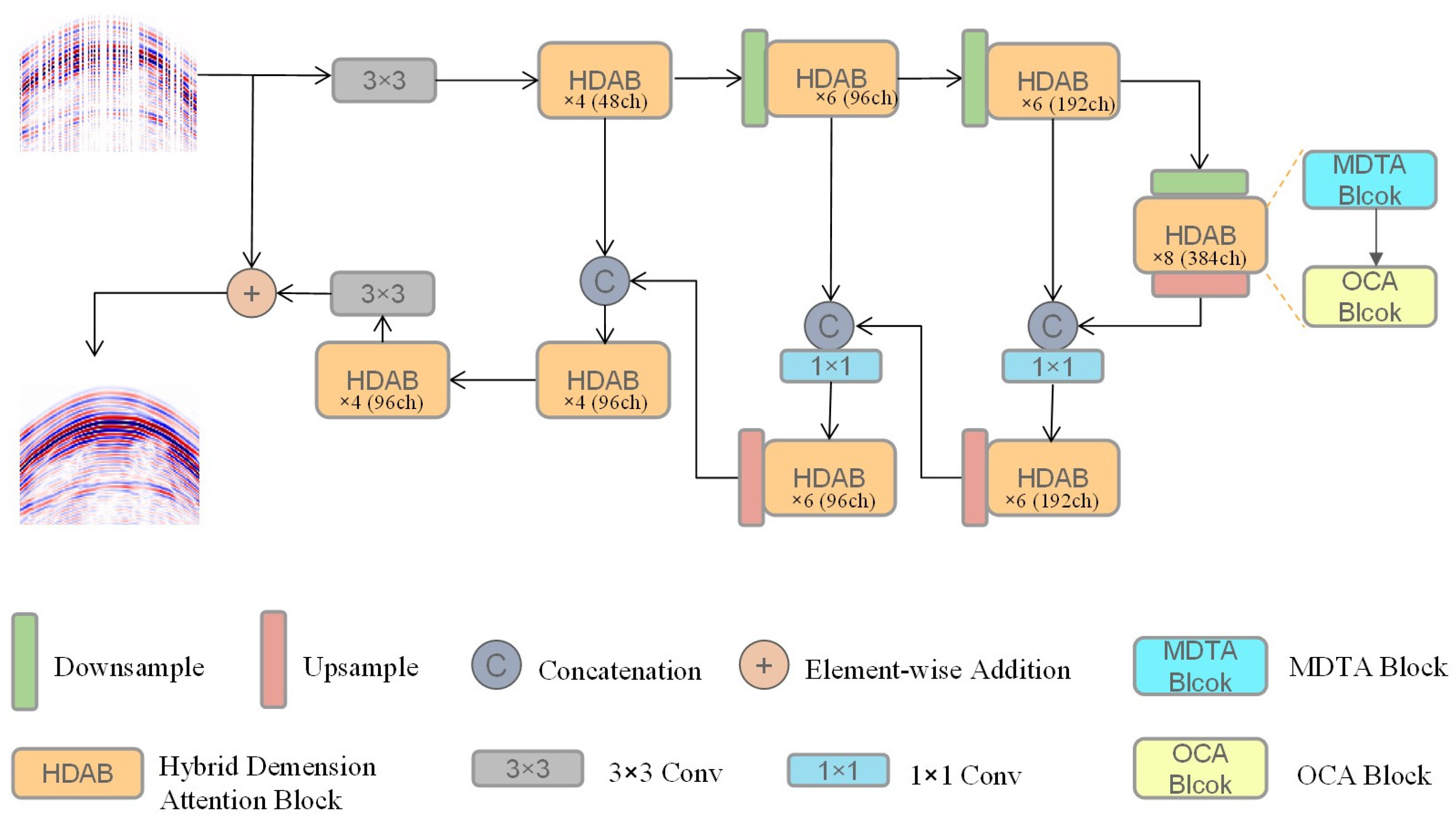
HDAR employs a U-shaped deep neural network architecture that processes large-scale inputs and preserves original seismic information through multi-level feature sampling. The network integrates two complementary attention mechanisms: the MDTA module and the OCA module. MDTA treats channel features as processing units (tokens) rather than traditional pixel-space elements, modeling dependencies between different feature channels to enhance representations of important channels while suppressing redundant information. This enables cross-channel interactions while preserving spatial structural integrity. OCA enhances cross-window feature interactions, strengthening local continuity in the spatial dimension and maintaining phase-axis coherence. Deep convolutional operations are extensively employed throughout the network to enhance spatial information interaction capabilities. The network architecture is illustrated in Figure 1.

Figure 1 illustrates the complete architecture of HDAR. Given seismic data with missing traces as input, a single 3 × 3 convolutional layer first extracts shallow feature representations with 48 channels. These primary features are then progressively transformed into deep features through a four-stage symmetric encoder–decoder. The encoder comprises four stages containing 4, 6, 6, and 8 HDABs with channel dimensions 48, 96, 192, and 384, respectively. Each encoder stage is followed by a downsampling operation that halves the spatial resolution while doubling the channel capacity; this hierarchical compression enlarges the receptive field and reduces computational redundancy, enabling the network to capture macroscopic wavefield trends within large consecutive gaps. The decoder symmetrically reconstructs high-resolution representations through three stages containing 6, 6, and 4 HDABs with 192, 96, and 96 channels, respectively. Each decoder stage is preceded by an upsampling operation that doubles the spatial resolution, restoring the original input dimensions for precise trace-level reconstruction.

Skip connections link each encoder stage to its corresponding decoder stage. The outputs are concatenated along the channel dimension and then passed through a 1 × 1 convolution that halves the channel count, except for the shallowest skip connection between the first encoder and decoder stages, where the concatenated 96-channel feature is preserved without reduction to retain fine-grained textural details. Following the decoder, an additional refinement stage of 4 HDABs at 96 channels further enhances boundary fidelity. A final 3 × 3 convolutional layer generates the residual data, which is added to the degraded input via element-wise addition to produce the final reconstruction. This residual formulation stabilizes training by allowing the network to learn the deviation from the incomplete input rather than the full data distribution.

2.1. Hybrid-Dimension Attention Block (HDAB) of Network

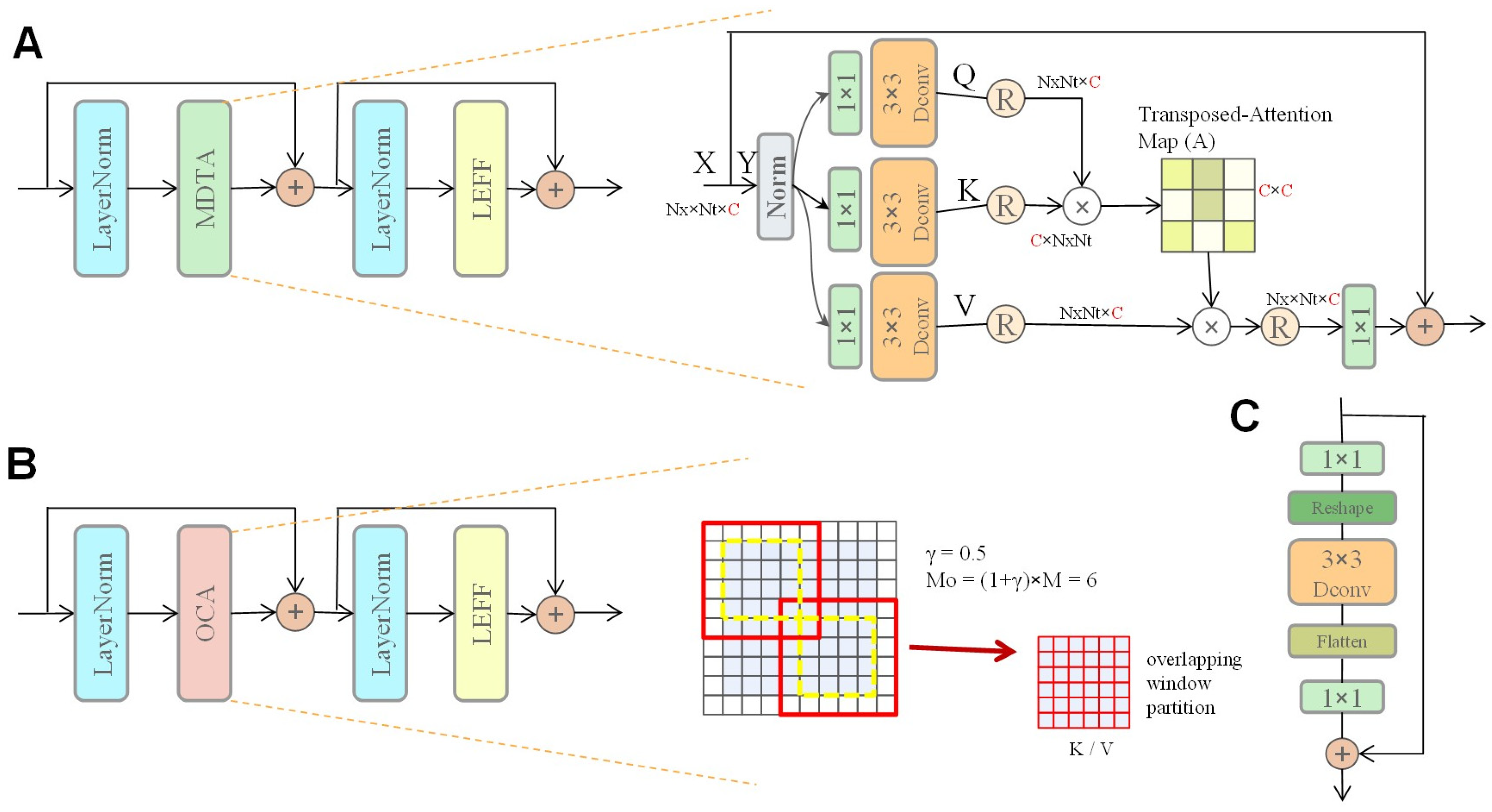
The hybrid-dimension attention block (HDAB) sequentially stacks two attention sub-blocks: an MDTA sub-block and an OCA sub-block. As shown in Figure 2A, the MDTA sub-block first applies layer normalization, then computes multi-dconv head transposed attention, and adds the result to the input via a residual connection. This is followed by another layer normalization and the locally enhanced feed-forward (LEFF) layer, whose output is again added via a residual connection. The OCA sub-block shown in Figure 2B follows the same structure, replacing MDTA with overlapping cross attention. Each sub-block therefore contains an attention module and a feed-forward layer, both wrapped by layer normalization and residual connections.

We employed the MDTA module to perform cross-channel feature extraction on missing seismic data. Compared to traditional Transformer networks, this approach significantly reduces computational complexity while capturing overall seismic data characteristics. However, this also leads to interpolation recovery relying more heavily on certain global features across the seismic data, potentially neglecting inter-channel relationships and fault boundary fidelity. This can easily result in poor co-axis continuity and artifacts. Therefore, to balance global and local features, we combined the OCA module—which focuses on local details—with MDTA. This approach achieves better results with only a slight increase in computational time. The internal structure of MDTA and its arrangement with OCA are shown in Figure 2, where each MDTA and OCA block is followed by a Feed-Forward Layer (FFN).

2.1.1. Multi-Dconv Head Transposed Attention Block

In seismic interpolation tasks, the input data forms a two-dimensional profile of size $N_x\times N_t$, where $N_x$ is the number of spatial traces and $N_t$ is the number of temporal samples per trace. The feature tensor $X\in {\mathbb{R}}^{N_x\times N_t\times C}$ contains $C$ channels along the feature axis, with spatial axis $N_x$ and temporal axis $N_t$.

For this feature tensor, standard self-attention first projects it into query, key, and value matrices $Q,K,V\in {\mathbb{R}}^{N_x{N}_t\times C}$. The dot product $Q_h{K}_h^T$ produces an attention map of size $\left(N_x{N}_t\right)\times \left(N_x{N}_t\right)$. The time complexity is $\mathcal{O}\left(\right(N_x{N}_t{)}^2\cdot d_k)$ per head and the memory complexity is $\mathcal{O}\left(\right(N_x{N}_t{)}^2)$. As the trace count or sampling rate increases, this quadratic cost quickly becomes prohibitive for high-resolution seismic data.

To avoid this bottleneck, we employ the MDTA module, which shifts attention computation from the spatial dimension to the channel dimension. Starting from the layer-normalized tensor $Y\in {\mathbb{R}}^{N_x\times N_t\times C}$, MDTA first generates query, key, and value projections enriched with local context. A $1\times 1$ pointwise convolution aggregates cross-channel information at each spatial position, followed by a $3\times 3$ depthwise convolution to encode local spatio-temporal features across channels. This yields $Q=W_d^Q\ast (W_p^Q\ast Y),K=W_d^K\ast (W_p^K\ast Y)$, and $V=W_d^V\ast (W_p^V\ast Y)$, where $\ast$ denotes the convolution operation, $W_p^{(\cdot )}$ denotes the $1\times 1$ pointwise convolution, and $W_d^{(\cdot )}$ denotes the $3\times 3$ depthwise convolution.

To compute the transposed attention and enhance representational capacity, MDTA partitions the $C$ channels into $H$ independent attention heads, each with a per-head dimension of $d_k=C/H$. For each head $h$, these contextual features are reshaped into head-specific matrices $Q_h\in {\mathbb{R}}^{N_x{N}_t\times d_k}$, $K_h\in {\mathbb{R}}^{d_k\times N_x{N}_t}$ (transposed), and $V_h\in {\mathbb{R}}^{N_x{N}_t\times d_k}$.

Instead of spatial interaction, the dot-product interaction generates a transposed attention map across the channel dimension for each head. The dot product $K_h\cdot Q_h$ involves matrices of dimensions $d_k\times \left(N_x{N}_t\right)$ and $\left(N_x{N}_t\right)\times d_k$, producing a head-specific attention map of size $d_k\times d_k$. This formulation reduces the overall complexity to $\mathcal{O}\left(C^2{N}_x{N}_t\right)$, which scales linearly rather than quadratically with the spatial resolution.

The outputs from all heads are concatenated along the channel dimension to restore the ${\mathbb{R}}^{N_x{N}_t\times C}$ shape, and projected back through a $1\times 1$ pointwise convolution $W_o\in {\mathbb{R}}^{C\times C}$ to fuse cross-head information. The overall MDTA process is formulated as:

$$\begin{array}{c}{\mathrm{h}\mathrm{e}\mathrm{a}\mathrm{d}}_{\mathrm{h}}={\mathrm{V}}_{\mathrm{h}}\cdot \mathrm{S}\mathrm{o}\mathrm{f}\mathrm{t}\mathrm{m}\mathrm{a}\mathrm{x}\left({\displaystyle \frac{{\mathrm{K}}_{\mathrm{h}}\cdot {\mathrm{Q}}_{\mathrm{h}}}{\mathrm{\sigma }}}\right)\end{array}$$

(2)

where the softmax is applied row-wise over the $d_k$ channel-token dimension.

$$\begin{array}{c}{\mathrm{X}}_{\mathrm{o}\mathrm{u}\mathrm{t}}=\mathrm{R}\mathrm{e}\mathrm{s}\mathrm{h}\mathrm{a}\mathrm{p}\mathrm{e}\left(\mathrm{C}\mathrm{o}\mathrm{n}\mathrm{c}\mathrm{a}\mathrm{t}({\mathrm{h}\mathrm{e}\mathrm{a}\mathrm{d}}_1,\dots ,{\mathrm{h}\mathrm{e}\mathrm{a}\mathrm{d}}_{\mathrm{H}})\cdot {\mathrm{W}}_{\mathrm{o}}\right)+\mathrm{X}\end{array}$$

(3)

where $X$ and $X_{out}$ are the input and output feature maps; $Q_h$, $K_h$, and $V_h$ represent the head-specific query, key, and value tensors for the $h$-th head, derived by reshaping and partitioning the contextual feature maps. Unlike the static scaling factor $\sqrt{d_k}$ used in standard self-attention, we explicitly employ a learnable parameter $\sigma$ to dynamically adjust the softmax temperature. This has been proven effective in channel-wise attention mechanisms to better optimize the magnitude of the dot product before normalization. After multiplying $V_h$ by the $d_k\times d_k$ attention map, the resulting tensor ${head}_h$ strictly maintains the dimension of $N_x{N}_t\times d_k$, preserving the spatial structure throughout the attention operation.

2.1.2. Overlapping Cross Attention Block

We introduce Overlapping Cross Attention (OCA) to strengthen local feature retention and cross-window correlation capabilities in seismic data. OCA operates as a cross-attention mechanism where query tokens from non-overlapping windows attend to key and value tokens from expanded overlapping neighborhoods. Given input features $\mathrm{X}\in {\mathbb{R}}^{{\mathrm{N}}_{\mathrm{x}}\times {\mathrm{N}}_{\mathrm{t}}\times \mathrm{C}}$, the OCA module operates in three successive steps: window partitioning, linear projection, and multi-head attention aggregation.

First, for window partitioning, the Query branch partitions $X$ into non-overlapping windows of size $M\times M$, yielding $N_w={\displaystyle \frac{N_x{N}_t}{M^2}}$ windows. Each local query feature $X_{Qi}$ thus has a flattened spatial dimension of $M^2\times C$. For the Key and Value branches, we extract overlapping blocks using a sliding window of size $M_o$ with stride $M$, padding edges with zeros to maintain consistent dimensions. This similarly yields $N_w$ overlapping windows, but each local key/value feature $X_{Ki}$ and $X_{Vi}$ has an expanded flattened spatial dimension of $M_o^2\times C$. The expanded window size $M_o$ is derived as:

$${\mathrm{M}}_{\mathrm{o}}=(1+\mathrm{\gamma })\times \mathrm{M}$$

(4)

where $\gamma$ is a constant controlling the overlap ratio.

Next, linear projections are applied to generate the query, key, and value matrices. Let H denote the number of attention heads, and $d_k=C/H$ denote the feature dimension per head. We compute:

$${\mathrm{Q}}_{\mathrm{i}}={\mathrm{X}}_{\mathrm{Q}\mathrm{i}}{\mathrm{W}}_{\mathrm{q}},\hspace{1em}{\mathrm{K}}_{\mathrm{i}}={\mathrm{X}}_{\mathrm{K}\mathrm{i}}{\mathrm{W}}_{\mathrm{k}},\hspace{1em}{\mathrm{V}}_{\mathrm{i}}={\mathrm{X}}_{\mathrm{V}\mathrm{i}}{\mathrm{W}}_{\mathrm{v}}$$

(5)

where $W_q, W_k,{ W}_v\in {\mathbb{R}}^{C\times d_k}$ are linear projection matrices.

Here, $Q_i\in {\mathbb{R}}^{M^2\times d_k},while K_i,V_i\in {\mathbb{R}}^{M_o^2\times d_k}$. Then, the cross-attention is computed as:

$$\mathrm{A}\mathrm{t}\mathrm{t}\mathrm{e}\mathrm{n}\mathrm{t}\mathrm{i}\mathrm{o}\mathrm{n}({\mathrm{Q}}_{\mathrm{i}},{\mathrm{K}}_{\mathrm{i}},{\mathrm{V}}_{\mathrm{i}})=\mathrm{s}\mathrm{o}\mathrm{f}\mathrm{t}\mathrm{m}\mathrm{a}\mathrm{x}\left({\displaystyle \frac{{\mathrm{Q}}_{\mathrm{i}}{\mathrm{K}}_{\mathrm{i}}^{\mathrm{T}}}{\sqrt{{\mathrm{d}}_{\mathrm{k}}}}}\right){\mathrm{V}}_{\mathrm{i}}$$

(6)

where the softmax is applied row-wise over the $M_o^2$ key dimension. The term $Q_i{K}_i^T$ generates an attention score matrix of size $M^2\times M_o^2$, representing the cross-attention weights between each query token and all key tokens in the expanded overlapping neighborhood. After multiplying by $V_i$, the resulting output for each window is $M^2\times d_k$, which is reshaped to $M\times M\times d_k$ and placed back into the non-overlapping query grid.

Finally, for multi-head aggregation, the outputs of $H$ independent attention heads are concatenated and projected:

$$\mathrm{M}\mathrm{S}\mathrm{A}\left(\mathrm{X}\right)=\mathrm{C}\mathrm{o}\mathrm{n}\mathrm{c}\mathrm{a}\mathrm{t}({\mathrm{h}\mathrm{e}\mathrm{a}\mathrm{d}}_1,{\mathrm{h}\mathrm{e}\mathrm{a}\mathrm{d}}_2,\dots ,{\mathrm{h}\mathrm{e}\mathrm{a}\mathrm{d}}_{\mathrm{H}}){\mathrm{W}}_{\mathrm{o}}$$

(7)

where ${head}_h=Attention(Q_{i,h},K_{i,h},V_{i,h})$ and $W_o\in {\mathbb{R}}^{C\times C}$ is the output projection matrix.

The window size $\mathrm{M}=8$ and overlap ratio $\mathrm{\gamma }=0.5$ are selected based on domain-specific validation and established architectural precedent. The value $\mathrm{M}=8$ matches the patch scale at which local waveform correlations are most pronounced in $128\times 128$ seismic blocks, as validated by preliminary grid search on the validation set. The overlap ratio $\mathrm{\gamma }=0.5$ provides sufficient overlap to suppress boundary artifacts without incurring the computational overhead of full-window overlap ($\mathrm{\gamma }=1.0$), consistent with the design rationale in the original Restormer and HAT architectures.

Consequently, during the attention calculation, each Query not only accesses information within its own $M\times M$ window but also establishes waveform propagation constraints from adjacent missing trace neighborhoods via the overlapping $M_o\times M_o$ regions. This explicitly enhances boundary fidelity for consecutive missing trace restoration and facilitates continuous phase axis reconstruction.

2.1.3. Locally Enhanced Feed-Forward Block

In seismic interpolation tasks, adjacent trace signals are crucial for reconstructing missing regions. However, the FFN in standard Transformers relies solely on global dot products, making it difficult to fully leverage local neighborhood information. To address this, we introduce a depthwise separable convolution module—Locally Enhanced Feed-Forward (LEFF) into the FFN. The workflow is as follows: first, a linear mapping layer expands the channel dimension, reshaping the one-dimensional track set tokens into a two-dimensional time-track matrix. Then, a $3\times 3$ per-channel convolution is applied to capture local geological correlations between adjacent sampling points and tracks. Subsequently, the two-dimensional features are flattened and restored to the original channel count. This design shown in Figure 2C preserves the global dependency advantages of transformers while significantly enhancing the ability to finely reconstruct consecutive or near-trace missing trace segments. We use GELU as the activation function after each linear/convolution layer.

2.2. Progressive Learning

The original Restormer employs a progressive strategy based on patch size, increasing from small to large blocks during training. Our approach instead varies the missing trace rate while keeping the seismic image size fixed at $128\times 128$. This directly targets the distribution of missing information in seismic data, where the challenge lies in the degree of undersampling rather than the spatial scale of the input.

Training begins with 10% irregularly missing data. At this stage, the network learns fine-grained local variations, such as small trace shifts and localized reflection characteristics. As the missing rate increases to 80%, the network must handle larger gaps and recover relationships between increasingly distant traces. We use only irregularly missing patterns throughout the curriculum; the model therefore generalizes from simple random gaps to severe consecutive missing without encountering the latter prematurely.

This schedule aligns with curriculum learning, where task complexity increases over time. The model first learns local trace recovery under well-constrained conditions, then progressively acquires the long-range dependencies needed for large consecutive gaps. In the later stages, exposure to higher missing rates enhances robustness against diverse patterns, enabling the network to restore large gaps and infer structural relationships between missing and valid traces.

Geophysical inverse problems are inherently ill-posed and highly non-convex. This curriculum acts as a dynamic regularization path: by optimizing for simpler, well-constrained scenarios initially, the network avoids poor local minima before tackling severely ill-posed reconstruction at high missing rates.

2.3. Network Training

The hyperparameters are determined through a two-stage procedure. The backbone architecture parameters, including channel dimensions, HDAB counts, and window settings, follow the Restormer [19] and HAT [20] configurations, which have been validated on high-resolution image restoration tasks with similar U-Net encoder–decoder structures. The training-specific parameters, including learning rate, batch size, and optimizer coefficients, are tuned via grid search on the validation set. The initial learning rate is selected from $\{5\times 10^{-5},10^{-4},2\times 10^{-4}\}$ based on the lowest validation loss after 20 epochs. The batch size is constrained to 4 by the 24 GB GPU memory limit. The weight decay 0.02 and AdamW momentum (0.9, 0.99) follow the standard practice in Transformer-based restoration networks.

Our synthetic datasets are sourced from publicly available benchmark models, including the SEG C3 dataset (45 shots, 8 ms sampling rate, 201 × 201 receiver grid, 625 samples per trace), the 1997 BP 2.5D migration benchmark model, the 2004 BP velocity estimation benchmark model, and the 2007 BP TTI velocity-analysis benchmark model. The field dataset is the Garben12 dataset. The dataset is partitioned at the shot-gather level: 70% of the shot gathers are allocated to the training set, 20% to the validation set, and 10% to the test set. Within each selected gather, traces are extracted and cropped into $128\times 128$ sub-blocks, yielding 27,960 sub-blocks in total. As described earlier, the data was normalized between 0 and 1 before input to the network. Specifically, this normalization was performed globally across the entire dataset by using the global maximum and minimum values. This ensures that the relative amplitude differences between different seismic traces are strictly preserved.

We employ the mean squared error (MSE) loss between the network output and the ground truth complete data as the training objective. For an input batch with ground truth $\mathrm{Y}$ and network output ${\mathrm{Y}}_{\mathrm{o}\mathrm{u}\mathrm{t}}$, the loss is computed as:

$$\begin{array}{c}\mathcal{L}={\displaystyle \frac{1}{\mathrm{N}}}{\displaystyle \sum _{\mathrm{i}=1}^{\mathrm{N}}}({\mathrm{Y}}_{\mathrm{i}}-{\mathrm{Y}}_{\mathrm{o}\mathrm{u}\mathrm{t},\mathrm{i}}{)}^2\end{array}$$

(8)

where $N$ is the number of pixels in the batch.

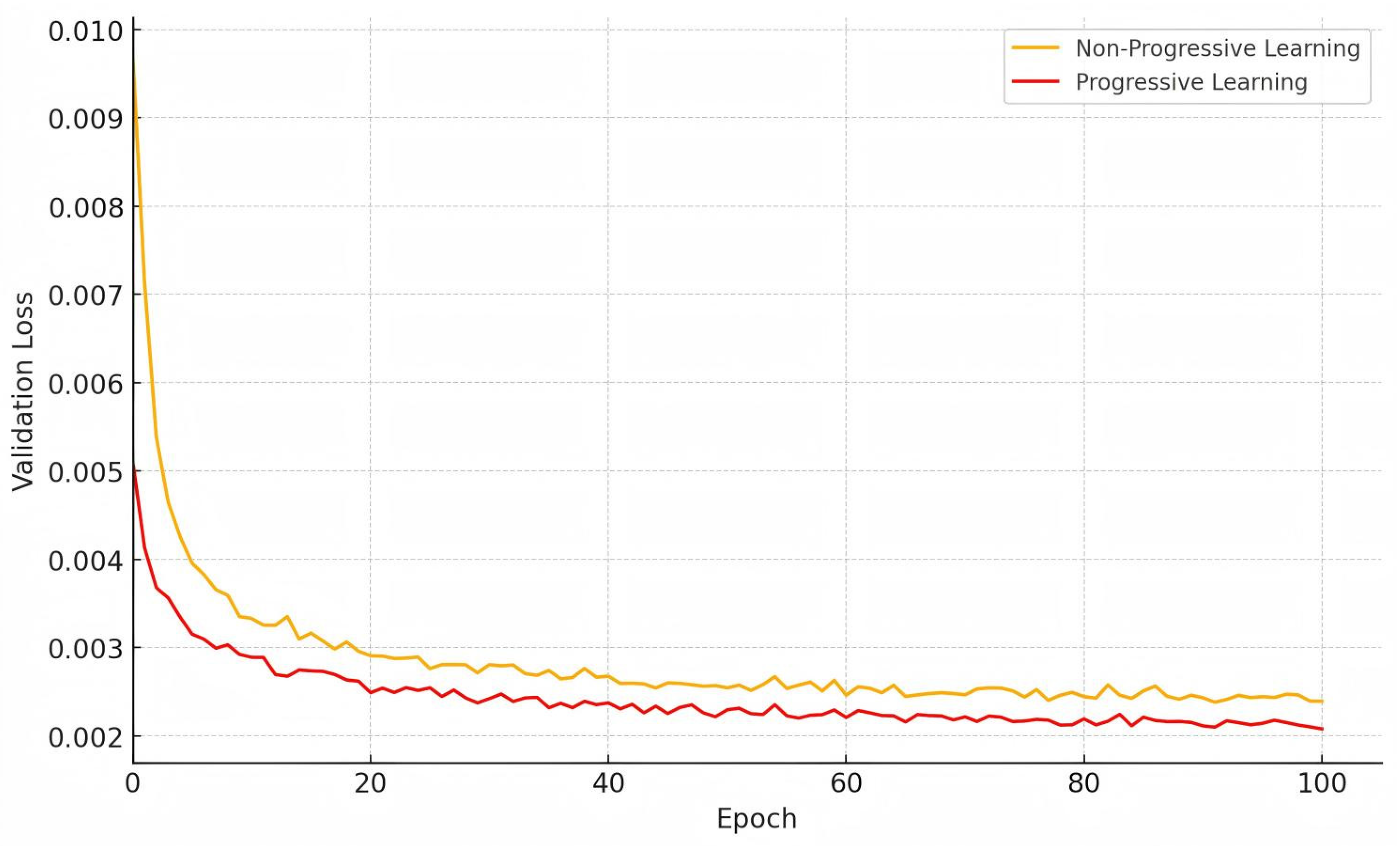
The AdamW optimizer [22] is selected, with momentum ranging from (0.9, 0.99); with a weight decay rate of 0.02. The learning rate update strategy employed cosine annealing, with initial and final learning rates set to 1 × 10⁻⁴ and 1 × 10⁻⁶, respectively. Each HDAB first computes channel attention on the feature map, then divides it into 8 × 8-sized windows with an overlap rate of 0.5, resulting in an effective window size of 12 × 12. The first convolutional layer of the HDAR has 48 channels; the training dataset batch size is set to 4, with a total of 100 training epochs. Each Transformer block in the network consists of multiple HDABs, with the number of HDABs being 4, 6, 6, 8, 6, 6, and 4 respectively. The training loss with and without progressive learning using the same validation data is shown in Figure 3. From the loss curve, it can be observed that the network using the progressive learning is more stable during training, and its loss is consistently lower than that of the network without progressive learning.

The total number of trainable parameters in the proposed HDAR model is approximately 26 million (26 M). This parameter scale strikes an optimal balance, ensuring sufficient model capacity to capture complex multi-dimensional seismic features without incurring prohibitive computational overhead.

All experiments were performed on an NVIDIA RTX 4090D GPU (NVIDIA Corporation, Santa Clara, CA, USA) with 24 GB of VRAM. The network was implemented in PyTorch (version 2.0, PyTorch Team, https://pytorch.org/, accessed on 15 May 2024) on Python (version 3.10, Python Software Foundation, https://www.python.org/, accessed on 15 May 2024). NumPy (version 1.24, NumPy Developers, https://numpy.org/, accessed on 15 May 2024) and Matplotlib (version 3.7, Matplotlib Development Team, https://matplotlib.org/, accessed on 15 May 2024) were used for data preprocessing and figure generation. Training each model to completion over 100 epochs required approximately 18 h.

3. Experiments and Results

3.1. Evaluation of Reconstruction Performance

We evaluate reconstruction quality using the signal-to-noise ratio (SNR), defined as:

$$\begin{array}{c}\mathrm{S}\mathrm{N}\mathrm{R}=10{\log }_{10}\left({\displaystyle \frac{\Vert \mathrm{Y}{\Vert }_2^2}{\Vert \mathrm{Y}-\hat{\mathrm{Y}}{\Vert }_2^2}}\right)\end{array}$$

(9)

where $Y$ denotes the ground truth complete seismic data, $\hat{Y}$ the reconstructed data, and $\Vert \cdot {\Vert }_2$ the $L_2$ norm. All SNR values reported in this study are computed with respect to this complete ground-truth data, which serves as the baseline for evaluating reconstruction quality. SNR measures the ratio of signal power to reconstruction error, yet it does not capture frequency characteristics, waveform variations, or spatial structure. These aspects are critical for seismic data because interpolation must preserve both signal strength and phase-axis continuity.

We supplement SNR with two qualitative assessments. Single-trace extraction selects one trace at a fixed spatial location and plots its amplitude against time, allowing point-by-point comparison of amplitude and phase between the original, undersampled, and reconstructed signals. This reveals waveform distortions and phase shifts that global metrics may obscure. Residual plots directly compare reconstruction errors across methods, highlighting differences in coherent event recovery and edge texture preservation.

The computational cost of HDAR remains moderate despite its attention mechanisms. MDTA reduces complexity to linear in spatial resolution, avoiding the quadratic cost of standard self-attention. Training time exceeds that of purely local CNNs such as UNet due to the attention and LEFF operations, yet remains comparable to the Swin Transformer. During inference, HDAR performs reconstruction in a single forward pass, offering deterministic efficiency.

3.2. Experiments on Synthetic Data

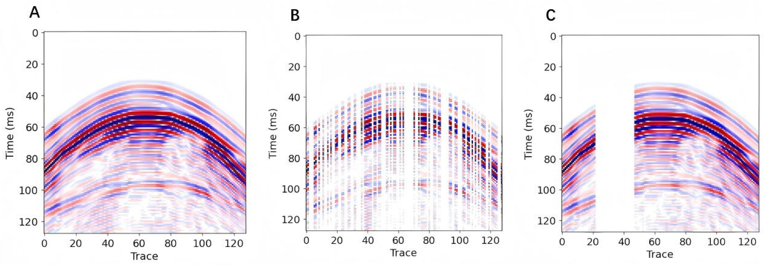
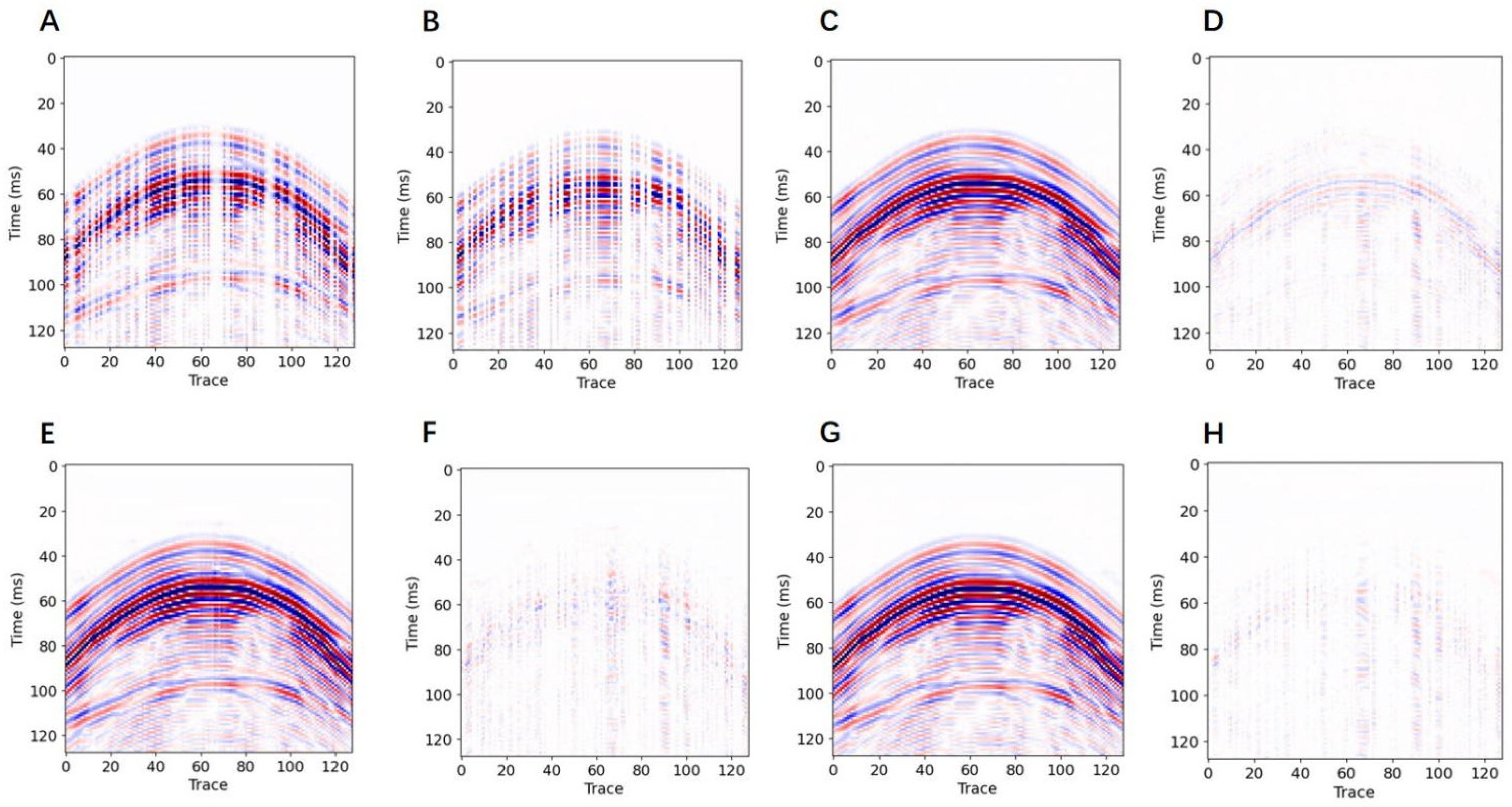
We evaluated the proposed method on the publicly available SEG C3 synthetic dataset. Figure 4 shows the complete data and the corresponding inputs with 50% irregularly missing traces and 20% consecutively missing traces. The reconstruction results and residuals are shown in Figure 5. For the irregularly missing case in Figure 4B, Framelet fails to close large gaps, producing visible energy loss in the scattered-wave region. UNet recovers the general waveform but introduces amplitude biases. The Swin Transformer reconstructs the main events yet leaves the later-arriving scattered waves incomplete. HDAR (Figure 5G,H) achieves lower residual magnitudes in the scattered-wave region than the competing methods.

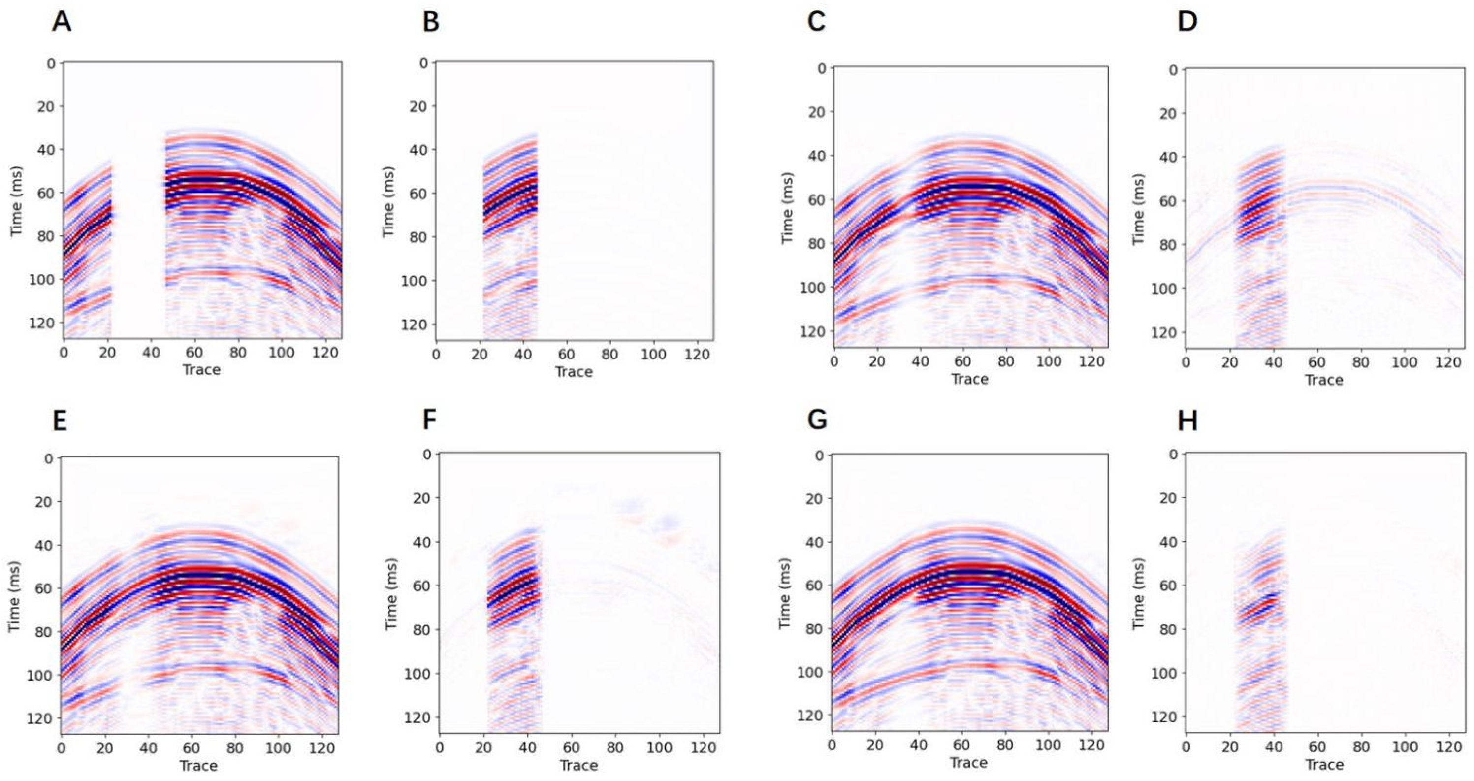
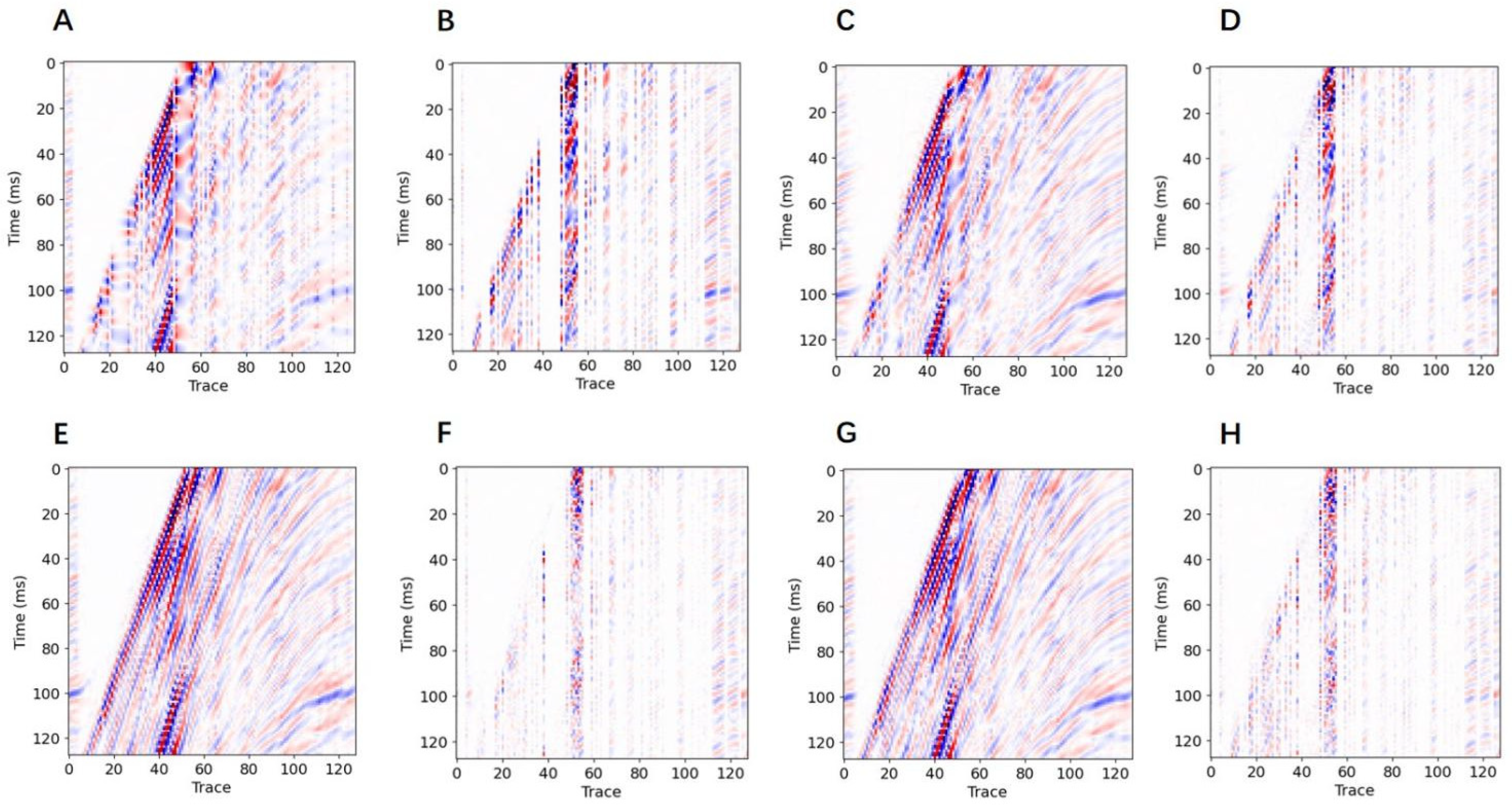
For the consecutively missing traces in Figure 4C, Framelet cannot recover the missing traces at all (Figure 6A). UNet restores only the edges of the gap, and its residual shows distorted waveforms with lost energy (Figure 6C,D). The Swin Transformer recovers the upper part of the gap yet leaves the later-arriving energy incomplete (Figure 6E). All methods preserve the primary arrivals with comparable fidelity; the advantage of HDAR is concentrated in the later-arriving scattered waves within large consecutive gaps.

Table 1. Comparison of SNR for synthetic data with different missing patterns.

Missing Type	Missing Data	Framelet	UNet	Swin Transformer	HDAR
Irregular	2.96	10.24	16.72	20.09	21.84
Consecutive	6.99	7.15	8.40	9.21	10.39

summarizes the SNR comparison. HDAR attains 21.84 dB for irregular missing patterns and 10.39 dB for consecutive gaps, outperforming the Swin Transformer by 1.75 dB and 1.18 dB, respectively.

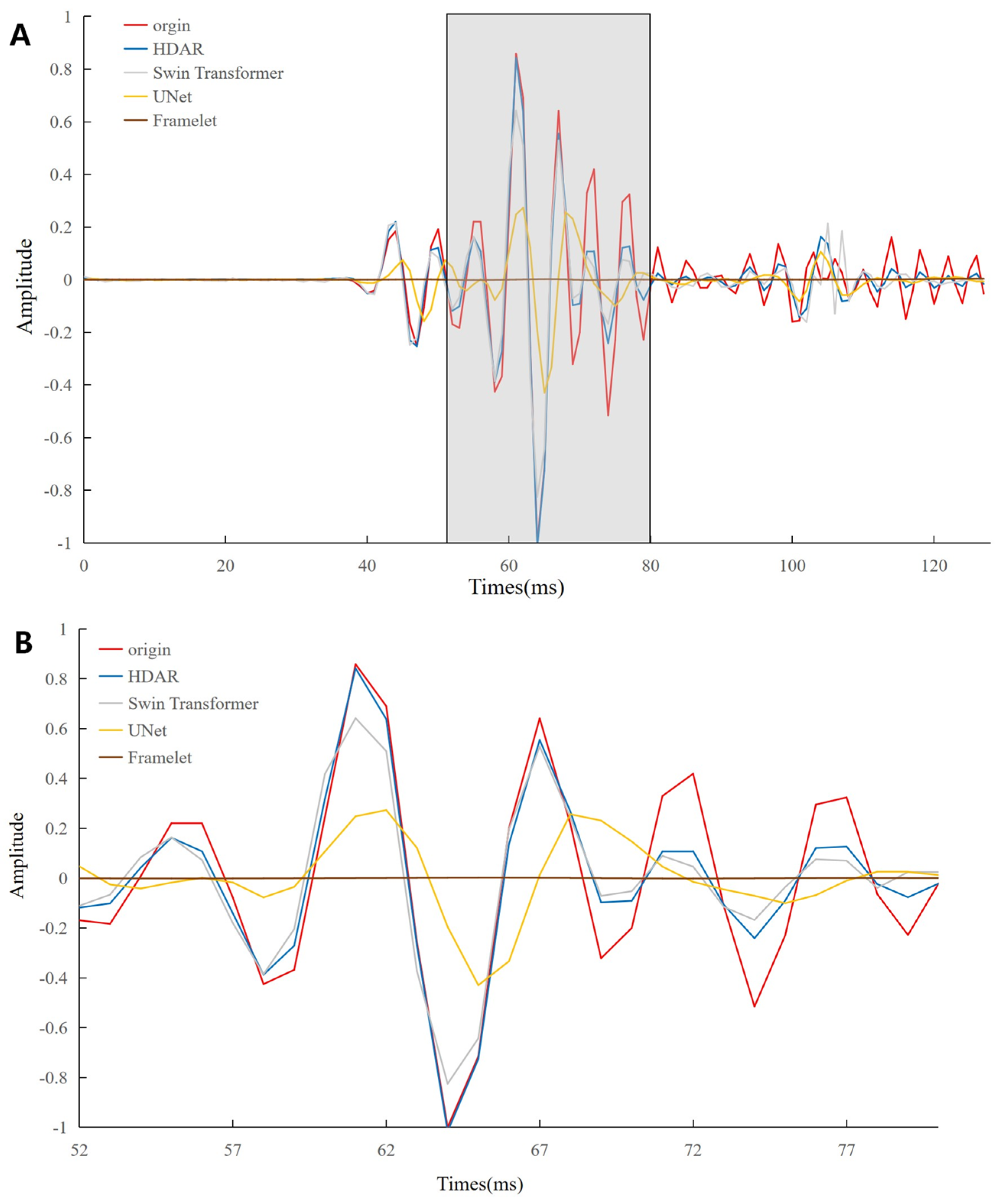
Figure 7A shows the reconstructed single trace for the irregularly missing case. The blue, gray, yellow, and brown lines correspond to the original data and the outputs of HDAR, Swin Transformer, UNet, and Framelet, respectively. Figure 7B magnifies the window marked in Figure 7A. In the later-arriving wave region (approximately 40–70 ms), the HDAR trace (blue) tracks the original (red) more closely than UNet and Framelet. All methods show comparable fidelity in the primary-arrival window (0–20 ms), indicating that the advantage of HDAR lies in the recovery of later-arriving energy.

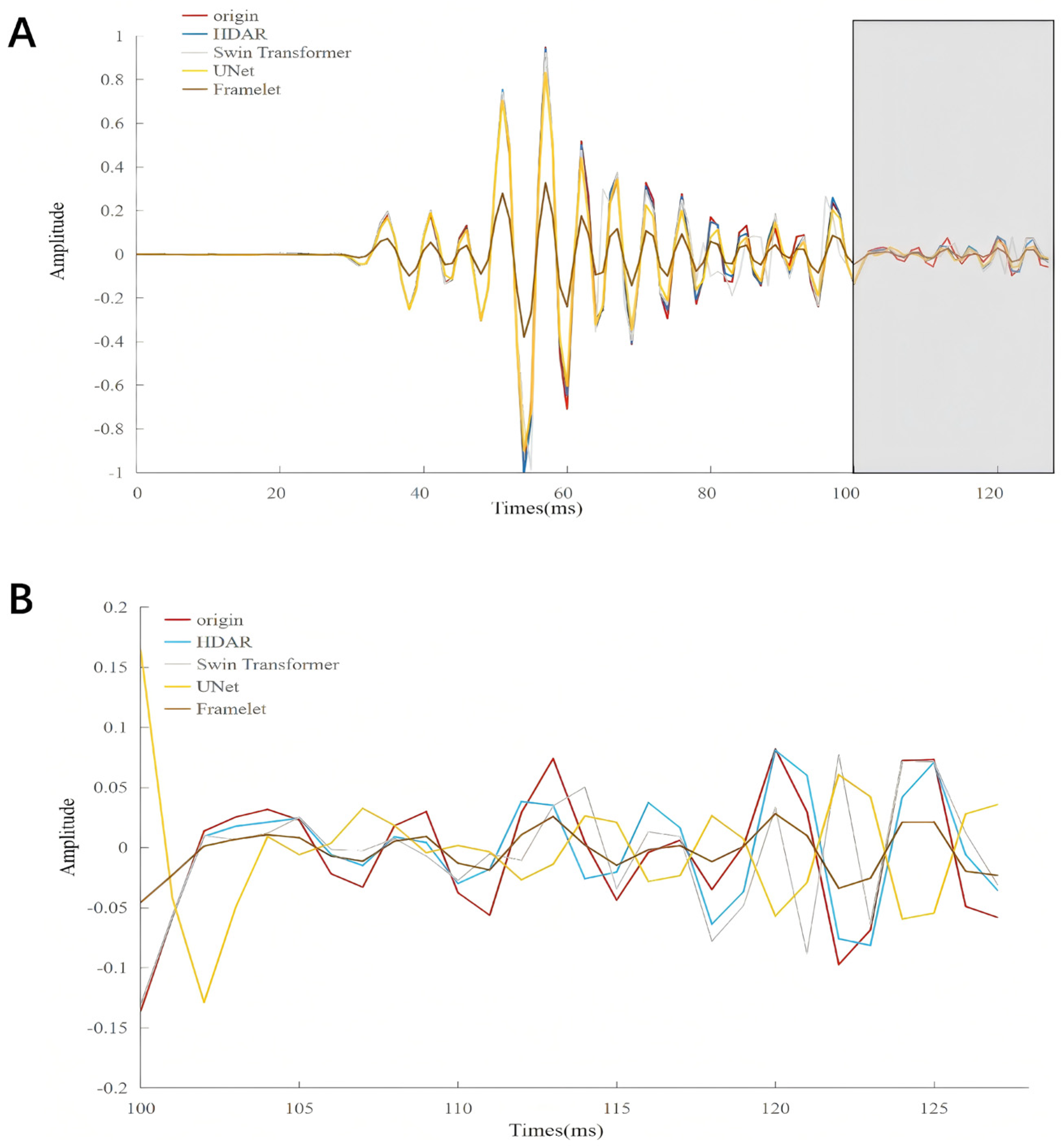
Figure 8A shows the reconstructed single trace for the consecutively missing case. Figure 8B magnifies the later-arriving wave window. HDAR remains closer to the original trace in this region, though none of the methods achieve perfect phase alignment.

Figure 7 and Figure 8 indicate that HDAR produces reconstructions closer to the original traces in the later-arriving wave regions for both irregularly and consecutively missing data. The hybrid attention design preserves scattered-wave features more effectively than Swin Transformer, UNet, and Framelet, particularly under large-scale missing patterns.

3.3. Experiments on Field Data

We conducted zero-shot tests on the Garben12 field dataset to evaluate cross-domain generalization. The model was trained exclusively on synthetic data without fine-tuning on field recordings.

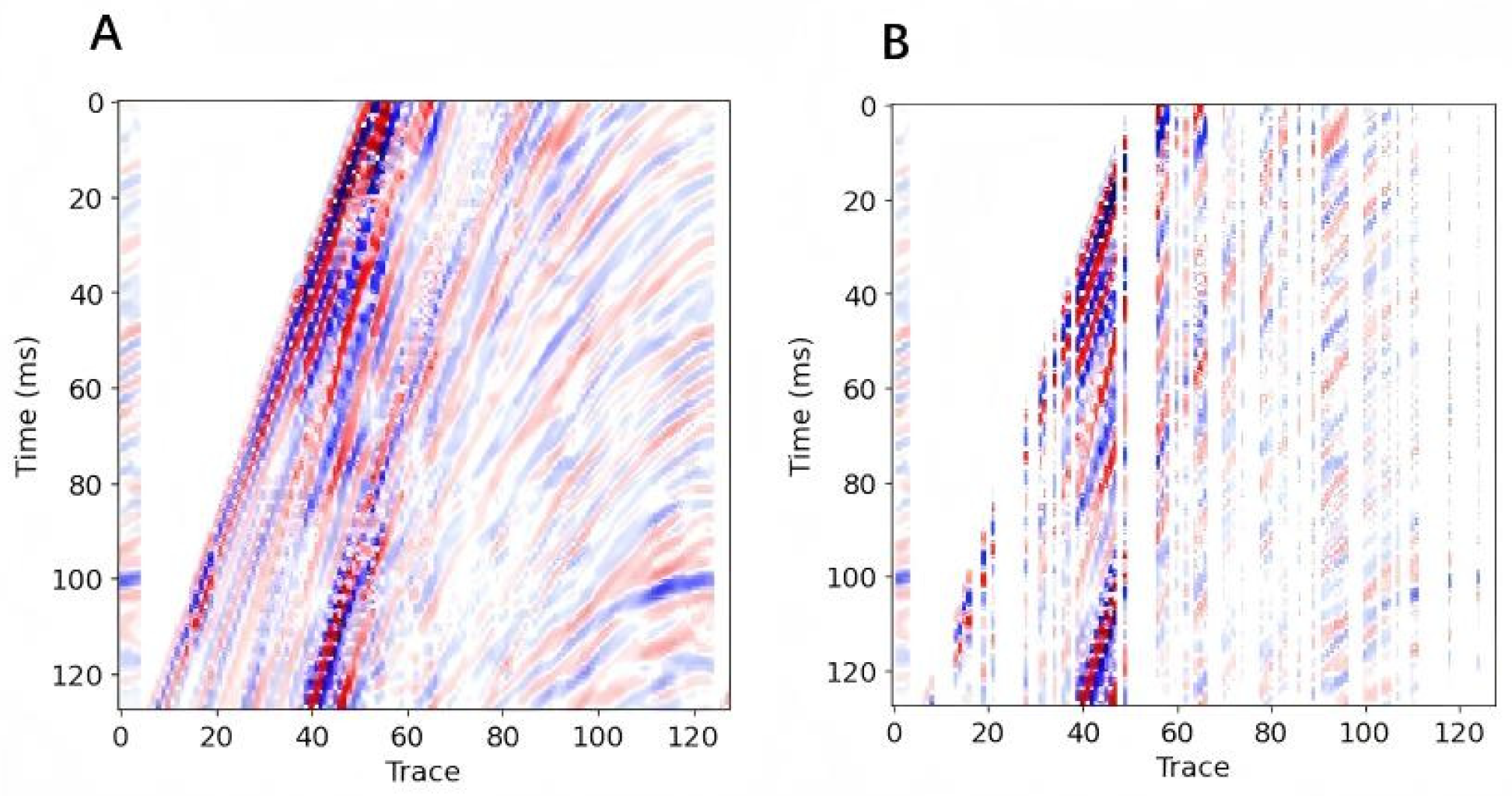
Figure 9 shows the original field data (A) and the input with 50% of traces irregularly removed (B). Figure 10 presents the reconstruction results and residuals. Field data reconstruction is inherently challenging due to ambient noise and subsurface heterogeneity, which produce subtle phase distortions across all methods. Framelet shows substantial energy loss (Figure 10A). UNet introduces visible global biases (Figure 10C). The Swin Transformer recovers the main events but leaves later-arriving energy incomplete (Figure 10E). HDAR (Figure 10G) preserves structural continuity in the later-arriving wave region more effectively than the competing methods, suppressing noise without excessive signal loss.

Table 2. Comparison of SNR for field data with irregular missing patterns.

Missing Type	Missing Data	Framelet	UNet	Swin Transformer	HDAR
Irregular	3.17	6.05	8.24	11.46	12.82

reports the SNR comparison for irregular missing patterns. HDAR attains 12.82 dB, exceeding the Swin Transformer (11.46 dB), UNet (8.24 dB), and Framelet (6.05 dB). This confirms that HDAR maintains a relative advantage in scattered-wave recovery on field data.

Large-scale consecutive gaps in field recordings involve spatial aliasing and near-surface scattering that exceed the current training framework. This study therefore focuses on irregular missing patterns, which dominate practical acquisition due to equipment failures and uneven geophone deployment.

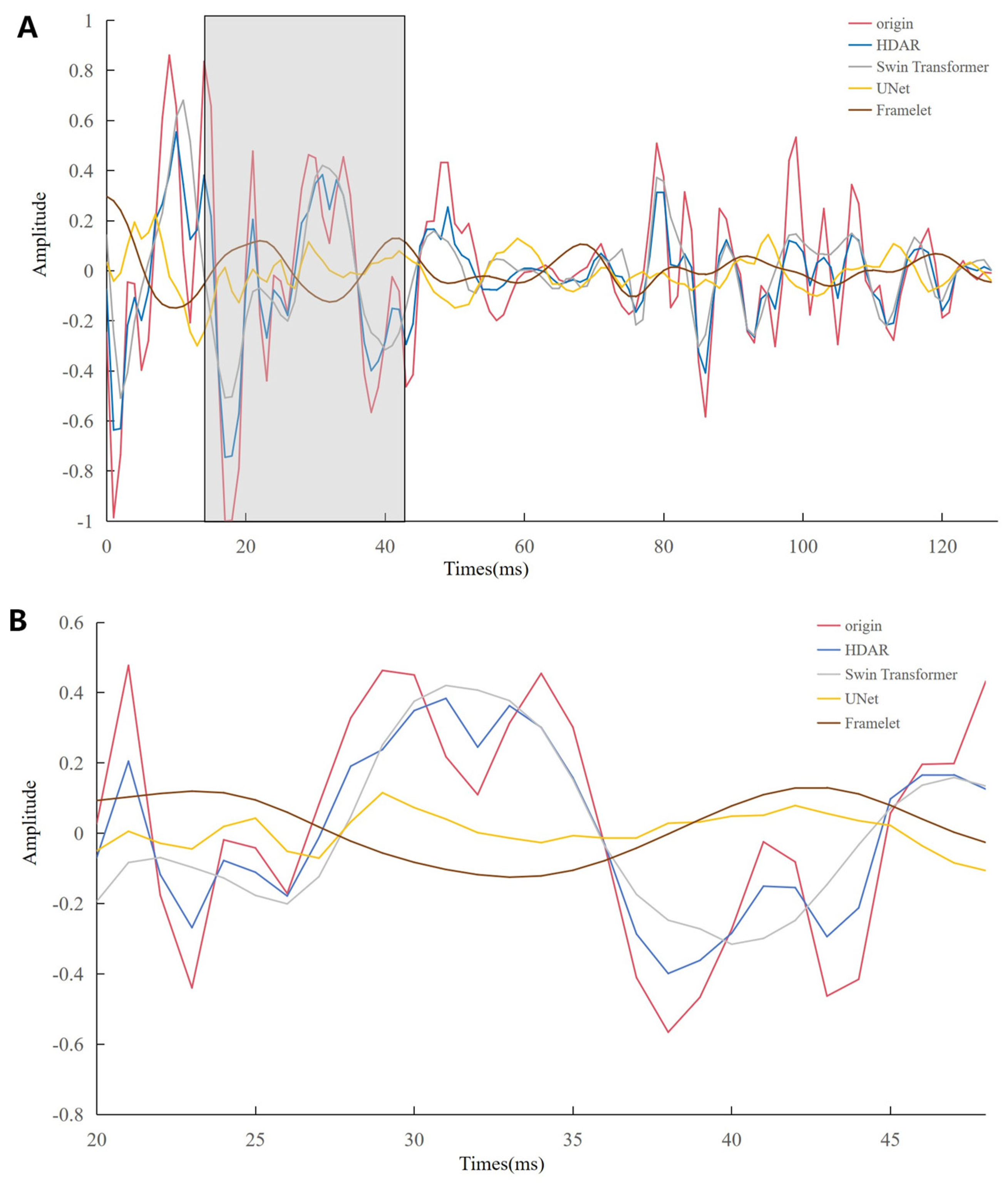
Figure 11A compares single traces for the irregularly missing field data. The blue, gray, yellow, and brown lines correspond to HDAR, Swin Transformer, UNet, and Framelet, respectively, against the original trace in red. Figure 11B magnifies the later-arriving wave window. HDAR tracks the original trace more closely than the other methods in this region. All approaches preserve the primary arrivals with comparable fidelity (approximately 0–20 ms); the advantage of HDAR is concentrated in the recovery of later-arriving energy under realistic conditions.

3.4. Ablation Study

To validate the contribution of each component, we conduct an ablation study on the SEG C3 dataset by progressively adding modules to the Restormer backbone.

Table 3. Ablation study on HDAR components on the SEG C3 dataset.

Configuration	MDTA	OCA	LEFF	Progressive Learning	Irregular (dB)	Consecutive (dB)
Unet	✗	✗	✗	✗	16.72	8.40
Restormer (baseline)	✓	✗	✗	✗	20.79	9.63
+ OCA	✓	✓	✗	✗	21.24	9.93
+ LEFF	✓	✓	✓	✗	21.53	10.15
HDAR (full)	✓	✓	✓	✓	21.84	10.39

reports the reconstruction SNR under irregular and consecutive missing patterns. The UNet baseline achieves 16.72 dB and 8.40 dB respectively, limited by its local receptive field. The Restormer baseline, which employs MDTA and a standard feed-forward layer, improves upon UNet by 4.07 dB and 1.23 dB, confirming that channel-wise global attention effectively captures cross-trace correlations at linear spatial complexity.

Adding OCA to the Restormer backbone yields a further gain of 0.45 dB on irregular missing data and 0.30 dB on consecutive gaps. The overlapping local windows enforce boundary fidelity at missing-trace edges where purely channel-wise attention tends to blur, which is critical for preserving phase-axis continuity in large consecutive gaps. Replacing the standard feed-forward layer with LEFF contributes a modest gain of 0.29 dB and 0.22 dB, reflecting the limited but non-negligible benefit of enhancing local trace correlations through depthwise separable convolutions. The progressive learning strategy provides a further gain of 0.31 dB and 0.24 dB, particularly for irregular missing patterns where the curriculum stabilizes training across diverse gap distributions. These additive gains indicate that OCA, LEFF, and PL each address a distinct limitation of the Restormer backbone, and the full configuration achieves measurable gains in both irregular and consecutive missing patterns.

4. Discussion

HDAR unifies global channel attention and local spatial attention within a single deterministic network. This differs from Swin Transformer-based methods [15], which rely on shifted non-overlapping windows that introduce boundary artifacts at large consecutive gaps and are optimized for simultaneous denoising rather than pure reconstruction. Diffusion-based methods [16] require tens to hundreds of iterative sampling passes, making them impractical for production workflows that demand deterministic single-pass inference. The original Restormer [19] provides the channel-attention backbone but lacks explicit spatial boundary refinement; when consecutive gaps exceed half the window size, reconstruction degrades at gap edges because channel-only attention cannot enforce pixel-level phase continuity. Traditional methods such as Framelet [7] and low-rank approximation [8] provide rigorous solutions under sparsity assumptions, yet these assumptions fail at high missing rates. Diffusion-based methods were not evaluated experimentally in this study, as their iterative sampling strategy—requiring tens to hundreds of forward passes per reconstruction—differs fundamentally from the deterministic single-pass framework we adopt.

The ablation study in Section 3.4 confirms that each component targets a distinct limitation. MDTA provides the dominant gain of 4.07 dB over the UNet baseline by capturing cross-trace correlations at linear complexity. OCA contributes 0.45 dB and 0.30 dB by enforcing boundary fidelity at missing-trace edges. LEFF adds 0.29 dB and 0.22 dB through depthwise separable convolutions, consistent with the limited but non-negligible role of local feed-forward mechanisms observed in the original Restormer. Progressive learning contributes 0.31 dB and 0.24 dB by stabilizing training across missing rates. In practice, irregular missing traces from equipment failure or uneven geophone deployment dominate land and marine acquisition. HDAR preserves later-arriving scattered-wave continuity under these conditions, which matters for high-resolution shallow exploration and VSP reconstruction. The SNR improvements over Swin Transformer (1.75 dB and 1.18 dB) are modest, as all methods approach the band-limited reconstruction limit under synthetic conditions; the advantage is clearer in scattered-wave recovery, where the hybrid design preserves phase continuity that windowed or channel-only methods miss. The ablation study in Table 3 is currently limited to the SEG C3 synthetic dataset. Extending this component-level validation to other benchmark models, including the BP 2004 and BP 2007 datasets, remains future work.

The current framework remains limited on field data with large consecutive gaps. Spatial aliasing, near-surface scattering, and non-stationary noise exceed the synthetic training distribution, and all tested methods degrade comparably in phase consistency. Future work will incorporate measured field noise into the training loss, investigate wave-equation regularization for large consecutive gaps, and extend the framework to memory-efficient 3D volume interpolation through patch-based attention tiling.

5. Conclusions

We presented the Hybrid-Dimension Attention Restormer (HDAR) for seismic data reconstruction, which unifies channel-wise global attention and overlapping local attention within a single deterministic network. On synthetic data, HDAR achieves competitive SNR and preserves later-arriving scattered-wave continuity more effectively than UNet, Framelet, and Swin Transformer. On field data, it maintains a relative advantage under irregular missing patterns, although all tested methods face challenges in ideal phase consistency due to real-world noise and subsurface heterogeneity. Future work will integrate field noise statistics into the training pipeline, investigate wave-equation regularization for large consecutive gaps, and extend the framework to memory-efficient 3D volume interpolation.

References

1. Jia, Y.; Ma, J. What Can Machine Learning Do for Seismic Data Processing? An Interpolation Application. Geophysics 2017, 82, V163–V177. [Google Scholar] [CrossRef] [Scilit]
2. Pawelec, I.; Wakin, M.; Sava, P. Missing Trace Reconstruction for 2D Land Seismic Data with Randomized Sparse Sampling. Geophysics 2021, 86, P25–P36. [Google Scholar] [CrossRef] [Scilit]
3. Naghizadeh, M.; Sacchi, M.D. F-x Adaptive Seismic-Trace Interpolation. Geophysics 2009, 74, V9–V16. [Google Scholar]
4. Claerbout, J.F.; Nichols, D. Interpolation beyond Aliasing by (t,x)-Domain PEFs. In Proceedings of the 53rd EAEG Meeting, Florence, Italy, 26–30 May 1991; p. cp-42-00001. [Google Scholar]
5. Ronen, J. Wave-Equation Trace Interpolation. Geophysics 1987, 52, 973–984. [Google Scholar] [CrossRef] [Scilit]
6. Fomel, S. Applications of Plane-Wave Destruction Filters. Geophysics 2002, 67, 1946–1960. [Google Scholar] [CrossRef] [Scilit]
7. Pan, X.; Wu, H.; Chen, Y.; Qin, Z.; Wen, X. The Interplay of Framelet Transform and lp Quasi-Norm to Interpolate Seismic Data. IEEE Geosci. Remote Sens. Lett. 2023, 20, 1–5. [Google Scholar] [CrossRef] [Scilit]
8. Wu, J.; Bai, M.; Zhang, D.; Wang, H.; Huang, G.; Chen, Y. Fast and Robust Low-Rank Approximation for Five-Dimensional Seismic Data Reconstruction. IEEE Access 2020, 8, 175501–175512. [Google Scholar] [CrossRef] [Scilit]
9. Chen, Y.; Chen, X.; Wang, Y.; Zu, S. The interpolation of sparse geophysical data. Surv. Geophys. 2019, 40, 73–105. [Google Scholar] [CrossRef] [Scilit]
10. Park, J.; Choi, J.; Seol, S.J.; Byun, J.; Kim, Y. A Method for Adequate Selection of Training Data Sets to Reconstruct Seismic Data Using a Convolutional U-Net. Geophysics 2021, 86, V375–V388. [Google Scholar] [CrossRef] [Scilit]
11. Fang, W.; Fu, L.; Zhang, M.; Li, Z. Seismic Data Interpolation Based on U-Net with Texture Loss. Geophysics 2021, 86, V41–V54. [Google Scholar] [CrossRef] [Scilit]
12. Li, X.; Wu, B.; Zhu, X.; Yang, H. Consecutively Missing Seismic Data Interpolation Based on Coordinate Attention Unet. IEEE Geosci. Remote Sens. Lett. 2022, 19, 1–5. [Google Scholar] [CrossRef] [Scilit]
13. Zhang, H.; Yang, X.; Ma, J. Can Learning from Natural Image Denoising Be Used for Seismic Data Interpolation? Geophysics 2020, 85, WA115–WA136. [Google Scholar] [CrossRef] [Scilit]
14. Guo, Y.; Fu, L.; Li, H. Seismic Data Interpolation Based on Multi-Scale Transformer. IEEE Geosci. Remote Sens. Lett. 2023, 20, 1–5. [Google Scholar] [CrossRef] [Scilit]
15. Gao, L.; Shen, H.; Min, F. Swin Transformer for Simultaneous Denoising and Interpolation of Seismic Data. Comput. Geosci. 2024, 183, 105510. [Google Scholar] [CrossRef] [Scilit]
16. Deng, F.; Wang, S.; Wang, X.; Fang, P. Seismic Data Reconstruction Based on Conditional Constraint Diffusion Model. IEEE Geosci. Remote Sens. Lett. 2024, 21, 1–5. [Google Scholar] [CrossRef] [Scilit]
17. Liu, Q.; Ma, J. Generative interpolation via a diffusion probabilistic model. Geophysics 2024, 89, V65–V85. [Google Scholar] [CrossRef] [Scilit]
18. Wang, S.; Deng, F.; Jiang, P.; Gong, Z.; Wei, X.; Wang, Y. SeisFusion: Constrained diffusion model with input guidance for 3-D seismic data interpolation and reconstruction. IEEE Trans. Geosci. Remote Sens. 2024, 62, 1–15. [Google Scholar] [CrossRef] [Scilit]
19. Zamir, S.W.; Arora, A.; Khan, S.; Hayat, M.; Khan, F.S.; Yang, M.H. Restormer: Efficient Transformer for High-Resolution Image Restoration. In Proceedings of the IEEE/CVF Conference on Computer Vision and Pattern Recognition (CVPR), New Orleans, LA, USA, 18–24 June 2022; pp. 5718–5729. [Google Scholar] [CrossRef] [Scilit]
20. Chen, X.; Wang, X.; Zhang, W.; Kong, X.; Qiao, Y.; Zhou, J. HAT: Hybrid Attention Transformer for Image Restoration. IEEE Trans. Pattern Anal. Mach. Intell. 2026, 48, 2676–2694. [Google Scholar] [CrossRef] [Scilit] [PubMed]
21. Bengio, Y.; Louradour, J.; Collobert, R.; Weston, J. Curriculum Learning. In Proceedings of the 26th Annual International Conference on Machine Learning, Montreal, QC, Canada, 14–18 June 2009; pp. 41–48. [Google Scholar] [CrossRef] [Scilit]
22. Loshchilov, I.; Hutter, F. Decoupled Weight Decay Regularization. In Proceedings of the 7th International Conference on Learning Representations, New Orleans, LA, USA, 6–9 May 2019; Available online: https://openreview.net/forum?id=Bkg6RiCqY7 (accessed on 26 May 2026).
Figure 1. The network architecture of HDAR.
Applsci 16 06589 g001
Figure 2. Structures of HDAR blocks. (A) Structure of MDTA Block. (B) The overlapping window partition for OCA Block. (C) Structure of LEFF.
Applsci 16 06589 g002
Figure 3. Validation loss with Progressive Learning or Non-Progressive Learning.
Applsci 16 06589 g003
Figure 4. Different missing patterns of synthetic seismic data. (A) Complete data; (B) irregularly missing data; (C) consecutively missing data.
Applsci 16 06589 g004
Figure 5. Reconstruction results and residual results of different methods in the synthetic dataset with irregularly missing traces. (A,B) Framelet; (C,D) UNet; (E,F) Swin Transformer; (G,H) the proposed method (HDAR).
Applsci 16 06589 g005
Figure 6. Reconstruction results and residual results of different methods in the synthetic dataset with consecutively missing traces. (A,B) Framelet; (C,D) UNet; (E,F) Swin Transformer; (G,H) the proposed method (HDAR).
Applsci 16 06589 g006
Figure 7. (A) Comparison of single-trace amplitude reconstruction on the synthetic seismic dataset with irregularly missing samples using Framelet, Swin Transformer, UNet, and the proposed method (HDAR). (B) Zoomed traces from the transparent gray window in (A).
Applsci 16 06589 g007
Figure 8. (A) Comparison of single-trace amplitude reconstruction on the synthetic seismic dataset with consecutively missing samples using Framelet, Swin Transformer, UNet, and the proposed method (HDAR). (B) Zoomed traces from the transparent gray window in (A).
Applsci 16 06589 g008
Figure 9. Different missing patterns of field seismic data. (A) Complete data; (B) irregularly missing data.
Applsci 16 06589 g009
Figure 10. Reconstruction results and residual results of different methods in the field dataset with irregularly missing traces. (A,B) Framelet; (C,D) UNet; (E,F) Swin Transformer; (G,H) the proposed method (HDAR).
Applsci 16 06589 g010
Figure 11. (A) Comparison of single-trace amplitude reconstruction on the field seismic dataset with irregularly missing samples using Framelet, Swin Transformer, UNet, and the proposed method (HDAR). (B) Zoomed traces from the transparent gray window in (A).
Applsci 16 06589 g011