Machine Learning-Based Forecasting of Indoor Microclimate Conditions for Heritage Conservation: A Case Study at the Archaeological Museum of Delphi

Abstract

Indoor environmental conditions must remain stable to preserve the cultural heritage objects exhibited in museums. Fluctuations in temperature and relative humidity accelerate degradation, and for this reason, their control is essential. Based on this, in this study, a machine learning-based framework for indoor microclimate forecasting is developed and evaluated, with application to the Archaeological Museum of Delphi. The analysis was based on indoor hourly temperature and relative humidity data from August 2022 to October 2024, combined with outdoor observational and ERA5-Land reanalysis data. Random Forest, Gradient Boosting and Support Vector Regression models were developed for 48 and 72 h forecast horizons. The RMSE, MAE, and R² methods were used to perform the model, while interpretability techniques, including Permutation Importance analysis and SHAP analysis, were also applied. The models successfully predicted indoor temperature with high accuracy, and the Gradient Boosting model demonstrated superior performance across all forecast horizons. Relative humidity proved to be more complex, with all models showing limited predictive skill. Overall, the findings highlight that temperature prediction depends on the building’s thermal inertia and historical values, while relative humidity is more sensitive to external and seasonal influences. Finally, this study demonstrates the potential of machine learning methods for forecasting microclimatic conditions in museum environments.

1. Introduction

The conservation of cultural objects is an important function of cultural heritage institutions, which include museums, historic buildings, libraries, and art galleries. These collections should be preserved over time and stable indoor environmental conditions, especially temperature and relative humidity, are of great importance in the successful long-term conservation of such collections [1,2]. Sudden or major changes in the inside climate can cause deterioration to occur more rapidly than can handling or direct exposure to the climate. For instance, high temperatures can cause chemical breakdown of organic materials, causing phenomena such as yellowing of paper, brittleness of parchment, and accelerated corrosion of metals. Relative humidity also has a significant influence, as high levels can encourage biological activity, and, in turn, the potential for biodeterioration. Over the last decade, moisture damage in buildings and technical systems has resulted in economic losses of billions of euros across Europe. Furthermore, excessive moisture accumulation within building envelopes can lead to the growth of mold, leading to poor indoor air quality and causing health problems for visitors and staff. Thus, the prediction of indoor relative humidity has become an important component in indoor air quality assessment and environmental control strategies [3,4].

To solve these problems, it is essential to understand indoor microclimate systems. The term describes the complete set of physical factors that control energy and mass movement in a closed space throughout its duration, with temperature and relative humidity serving as the main elements [5]. Traditional methods for assessing indoor microclimates often depended on fixed threshold values and long-term averages. However, recent studies have shown that these methods might not accurately reflect the changing environmental conditions affecting heritage collections. As a result, newer approaches have been created to consider temporal variability and the cumulative effects of environmental stressors on material degradation. Since indoor conditions are influenced by several interacting factors, including building characteristics, outdoor weather, HVAC operation, lighting, and visitor activity, continuous monitoring and predictive methods have become more important [6]. Therefore, it is important to monitor these conditions continuously to identify the critical conditions and mitigate the accelerated deterioration [7]. Seasonal variations, particularly during summer heatwaves and winter cold periods, pose additional risks, especially for sensitive materials such as stone and metals [7].

Heritage building monitoring shows temperature and humidity that exceed established levels because their environmental control systems do not provide proper atmospheric conditions. Although immediate visible damage may not be visible, prolonged exposure to adverse conditions can lead to cumulative degradation, including surface crusting, material delamination, and alterations at the interface between the original and restored elements [7]. Climate change is making these issues more severe. The problem of excessive heat during summer and extreme dryness during winter has grown worse for historic buildings, which have inadequate insulation, low thermal mass, and deteriorating exterior walls [8,9]. Rapid fluctuations in indoor conditions are particularly detrimental, as many collections have acclimated to historically stable microclimates. Consequently, precise monitoring and assessment are imperative not only for the preservation of artifacts but also for maintaining the structural and cultural integrity of heritage buildings [9].

Traditionally, environmental monitoring in museums has relied on continuous measurements of temperature and relative humidity, followed by retrospective analysis of climate curves and threshold exceedances [10,11,12]. Modern HVAC systems can create automatic alerts, but their functions operate as reactive systems that only activate when systems experience failures, which lead to permanent harm [13]. The monitoring system becomes less efficient because historic and monumental buildings face two main challenges, which include their thick masonry, their complex architectural designs, and their restricted areas for sensor installation. The environmental conditions become unstable because building elements, which include extensive glass windows and direct sunlight and heat created by visitors and nonoperational passive climate control systems, cause environmental conditions to approach dangerous thresholds during extreme weather situations [8,9]. Current standards for indoor microclimate management remain fragmented, and prevailing practice is strict HVAC-based control or adaptive strategies based on historically stable conditions that define acceptable ranges, but rarely provide tools for predicting future environmental states [6,14,15].

The continuous environmental data can be used to predict indoor temperature and relative humidity. Machine learning (ML) techniques are particularly suitable for such applications because they can capture complex, nonlinear relationships among environmental variables and have demonstrated strong performance in forecasting tasks, including weather prediction and building performance modeling [16]. While ML has been widely applied in cultural heritage research for image analysis, object classification, and condition assessment, recent advances in artificial intelligence have also enabled applications in knowledge extraction, decision support, and automated interpretation of complex information sources [17,18]. Nevertheless, the use of ML for forecasting indoor microclimate conditions remains relatively limited. Current research predominantly addresses anomaly detection or retrospective risk assessment, leaving predictive modeling for preventive conservation underdeveloped [19,20,21]. Time-series ML models can be used to provide early warnings of the critical conditions based on the correlations between the current and historical environmental state, which can help decision-makers with proactive actions [9,13,22].

In this context, the present work develops and evaluates a machine learning-based approach to predict the indoor microclimate of the Archaeological Museum of Delphi based on multiple data sources. The proposed approach combines indoor monitoring data, external observations, and ERA5 reanalysis data to explore the predictability of indoor temperature and relative humidity at 48 h and 72 h horizons, supporting early warning strategies for preventive conservation. Furthermore, the framework includes interpretability analysis so as to determine the most important environmental and temporal factors impacting the dynamics of the indoor climate.

The main innovative aspect of this research is not the development of a new machine learning (ML) model. Rather, the contribution of the study lies in the integration of three complementary types of datasets, namely indoor monitoring data, outdoor meteorological observations, and ERA5 reanalysis data, in a way that is suitable for addressing an ongoing environmental management problem at the Archaeological Museum of Delphi. The study also links forecast evaluation, early-warning capabilities, and interpretability analysis in order to provide information that can support museum staff in preventive conservation and decision-making processes. Therefore, rather than being fundamentally novel in terms of ML model development, this work should be viewed as an empirically validated case study of the Archaeological Museum of Delphi and as an integrated forecasting and evaluation framework for heritage microclimate management. In addition, the baseline comparisons and the relative humidity (RH) forecasting results provide useful insights into the practical limitations of current monitoring data and indicate where additional variables and more advanced modeling approaches may offer further improvements under real-world museum conditions.

Accordingly, the study is guided by the following research questions: (i) to what extent indoor temperature and relative humidity can be forecast at 48 h and 72 h horizons in the Delphi museum, (ii) which machine learning model class (Random Forest, Gradient Boosting Machine, or Support Vector Regression) performs best across variables and forecasting horizons, and (iii) which environmental variables and temporal signatures drive model predictions and whether these can be interpreted in a conservation context.

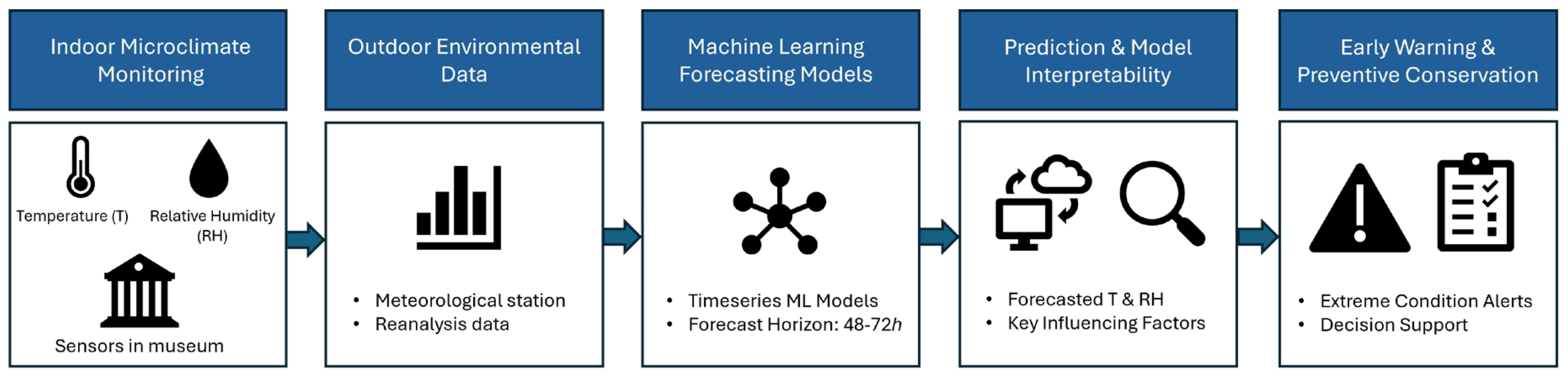
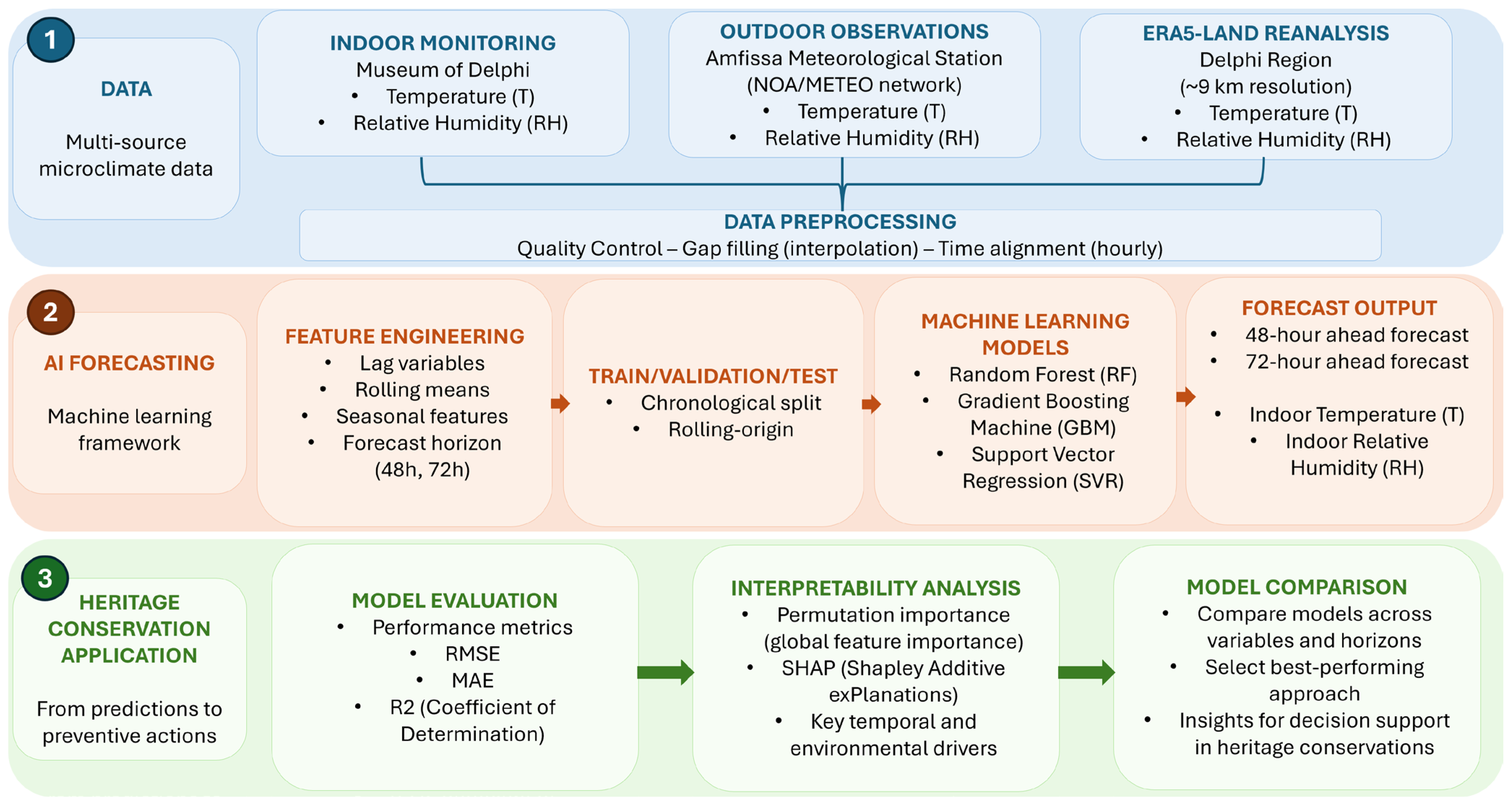
The proposed framework uses continuous environmental monitoring data together with machine learning methods to identify indoor microclimate conditions that might create dangerous situations. The proposed system combines short-term forecasting, interpretability analysis, and alert mechanisms in order to support real-time decision-making by museum professionals. It also helps improve the understanding of indoor microclimate conditions and supports preventive conservation strategies, enabling heritage institutions to better manage environmental risks. The AI-based tools enable monitoring to connect with preventive measures which protect delicate cultural heritage items while providing comfortable visitor experiences. The overall workflow of the proposed ML-based indoor microclimate forecasting and early-warning framework is shown in Figure 1.

Section 2 presents the data and methods used in the study and introduces the AI-based forecasting methodology, feature engineering, model selection, and interpretability techniques. In Section 3, the analysis results are presented, while Section 4 establishes the scientific knowledge base together with its associated limits and practical uses for cultural heritage management. Finally, the conclusions and the perspectives of the study are provided in Section 5.

2. Materials and Methods

2.1. Study Area

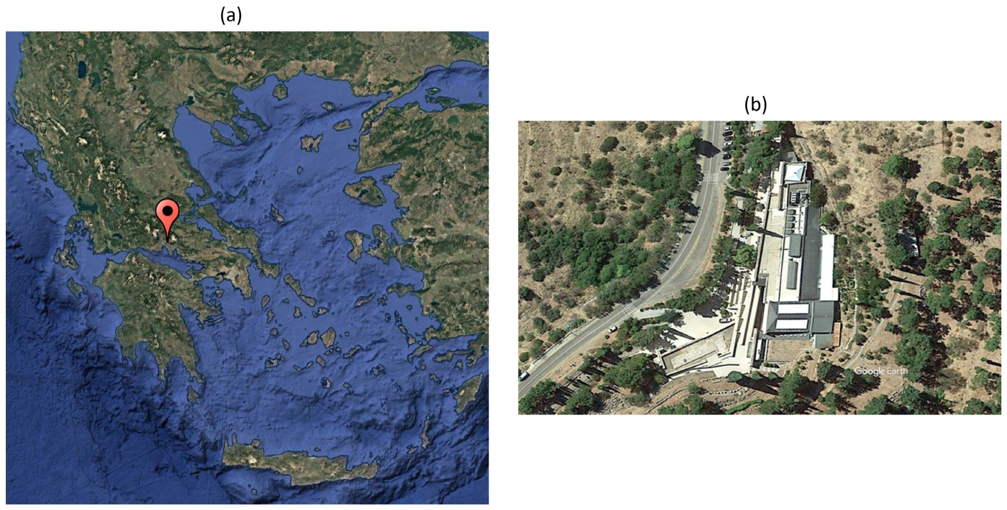
The region of Delphi in Greece is the study area of the present work. Delphi is located on the slopes of Mount Parnassus, between the Phaedriades cliffs, in the regional unit of Phocis, north of the Gulf of Corinth (Figure 2). The museum studied, the Delphi Archaeological Museum, is located in the archaeological site of Delphi, which is one of the most important monuments of the ancient Greek cultural heritage. It is located at 38°28′48″ N, 22°30′0″ E, at an elevation of approximately 560 m above sea level. Founded in 1903 and having undergone several renovations. It is currently housed in a two-story building with a total floor area of 2270 m², while its permanent exhibition is arranged across fourteen galleries. The collections mainly comprise architectural sculptures, statues, and small-scale artworks originating from the Delphic Sanctuary. The local climate of the area is classified as continental, characterized by hot and dry summers and cold, prolonged winters.

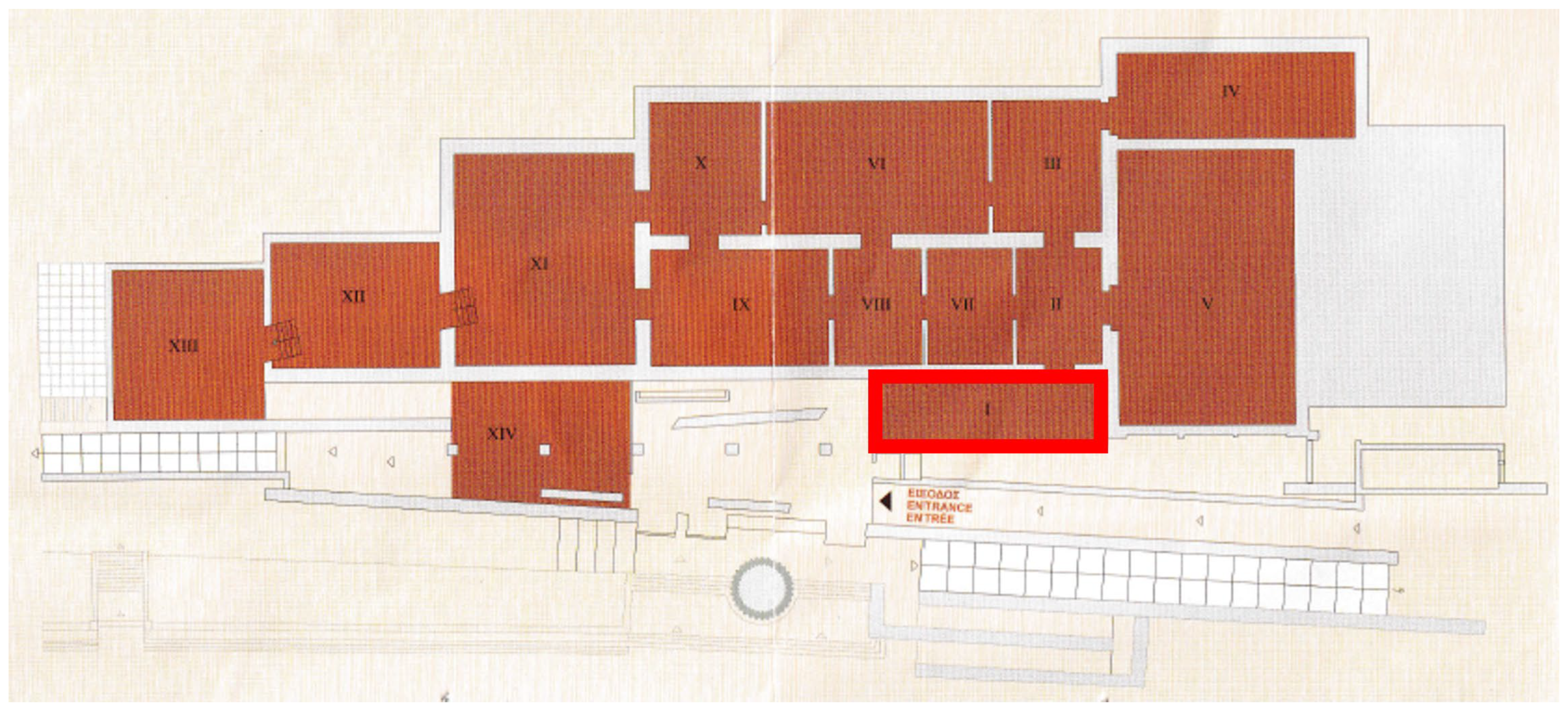
To ensure appropriate environmental conditions for exhibit conservation and thermal comfort for staff and visitors, the museum’s indoor microclimate is regulated by HVAC systems. This research focuses on Gallery I, “The Beginning of the Sanctuary,” the museum’s first exhibition space. It hosts artifacts primarily made of inorganic materials, such as bronze, displayed both inside and outside showcases. As shown in the floor plan (Figure 3), Gallery I is directly connected to the main entrance and to adjacent galleries V and XIV, allowing visitor circulation and potential airflow between exhibition spaces. The gallery’s front façade features a glazed wall that admits direct solar radiation, influencing temperature and relative humidity conditions within the space. It was selected for study due to its location at the building entrance, where the microclimate is particularly sensitive to high visitor traffic and temperature fluctuations caused by frequent door opening.

2.2. Data

2.2.1. Indoor Data

A long-term monitoring campaign spanning 27 months (August 2022–October 2024) was conducted to assess the indoor climate of the study room (Gallery Ι) at the Archaeological Museum of Delphi. The sensors were installed at a height of 2 m in places where they did not disturb the exposition of artifacts and were not exposed to theft or damage (e.g., on showcases). The sensors were installed at a height of 2 m and recorded temperature (T) and relative humidity (hereafter RH) hourly. The instruments were Extech RHT20 Humidity and Temperature Dataloggers (Extech Instruments, Nashua, NH, USA), with temperature measurements ranging from −40 to 70 °C (accuracy ± 1 °C for −10 to 40 °C, ±2 °C otherwise) and RH measurements from 0 to 100% (accuracy ± 3% at 40–60%, ±3.5% at 20–40% and 60–80%, ±5% at 0–20% and 80–100%), both with a resolution of 0.1 °C/0.1%.

2.2.2. Outdoor Data

Regarding the outdoor environment, hourly observational data from the Amfissa meteorological station were obtained from the National Observatory of Athens meteorological network [23]. The station, located at an altitude of 168 m above sea level, records temperature and RH at a height of 2 m above the ground surface. It is located approximately 11 km (linear distance) from the Archaeological Museum of Delphi. Considering the spatial and altitudinal differences between the meteorological station and the study area, deviations may occur due to local topographic and microclimatic effects. For this reason, the ERA5-Land reanalysis dataset for the Delphi region was also used, in addition to the observational data, to better represent the outdoor climatic conditions at the study site.

ERA5-Land is a high-resolution reanalysis dataset, offering hourly data on the surface over many decades, at a spatial resolution of ~9 km. The dataset is simulated from the land component of the ECMWF ERA5 climate reanalysis, providing a consistent, spatially coherent land surface dataset. All datasets had been time-aligned to a common resolution (hourly), and inconsistencies in the timestamps were corrected. Interpolated data were used to replace missing values, and an erroneous value or an obvious data outlier were eliminated after the data quality control process. Finally, both indoor and outdoor datasets were combined into a single time-series dataset for use in the analysis and modeling.

2.2.3. Exploratory Data Analysis

A comprehensive analysis of the museum’s indoor microclimate data, including the identification of temporal variability, extreme events, and indoor–outdoor relationships, was previously conducted in a dedicated study [24]. For the temperature, the results showed a pronounced seasonal variability, with higher indoor temperatures during the summer months, particularly in July. In terms of daily trends, the temperature tends to rise during museum hours, particularly in the morning. This suggests the influence of occupancy, system operation, and outdoor temperature conditions. Furthermore, a strong positive correlation was found between internal and external temperature. In contrast, RH showed greater variability and a weaker connection with external conditions. Overall, these findings provide the physical and statistical basis for the development of the machine learning framework in the present study.

2.3. Forecasting and Machine Learning Framework

This work aims to predict the indoor temperature and RH at the Archaeological Museum of Delphi over 48 h and 72 h horizons, using indoor monitoring data, outdoor observations, and ERA5 reanalysis data (Section 2.2). To achieve this, we compare multiple Machine Learning (ML) methods (Random Forest, Gradient Boosting, SVR) in order to support the development of an early warning system for preventive conservation decisions. The proposed machine learning includes chronological splitting into training, validation, and testing sets, together with rolling-origin cross-validation for additional robustness checks. Figure 4 presents the technical machine learning pipeline underlying the system, presented in Figure 1, outlining the full workflow from data preprocessing to model interpretation for reproducible implementation.

To preserve the temporal structure of the dataset and avoid information leakage, all observations were maintained in chronological order throughout model development. For each forecasting horizon, the first 70% of usable observations were allocated to the training set, the subsequent 15% to the validation set, and the remaining 15% to an independent test set. No random shuffling or random assignment of observations was performed at any stage of the analysis.

Table 1. Exact chronological split boundaries and sample sizes. Definitions of all variables and methodological terms are provided in Appendix A.

horizon_hours	train_start	train_end	valid_start	valid_end	test_start	test_end	n_train	n_valid	n_test
48	6 August 2022 16:00:00	29 February 2024 01:00:00	29 February 2024 02:00:00	30 June 2024 12:00:00	30 June 2024 13:00:00	30 October 2024 23:00:00	13,714	2939	2939
72	6 August 2022 16:00:00	28 February 2024 08:00:00	28 February 2024 09:00:00	29 June 2024 15:00:00	29 June 2024 16:00:00	29 October 2024 23:00:00	13,697	2935	2936

presents the chronological train–validation–test split and the corresponding sample sizes for each forecasting horizon. Model robustness was further evaluated using an expanding-window rolling-origin cross-validation strategy. For each forecasting horizon, two validation folds were constructed. In each fold, all observations preceding the validation period were used for training, while the validation window remained fixed. Consequently, the training dataset progressively expanded from one fold to the next, reflecting realistic forecasting conditions in which only past information is available at the time of prediction.

Table 2. Exported expanding-window rolling-origin fold configuration. Definitions of all variables and methodological terms are provided in Appendix A.

horizon_hours	train_start	train_end	valid_start
48	1	9159	1665
48	2	14,988	1665
72	1	9147	1663
72	2	14,969	1663

summarizes the rolling-origin fold configuration and the corresponding sample sizes for each forecasting horizon.

The framework transforms hourly indoor and outdoor observations into 48 h and 72 h ahead forecasts, using Random Forest (RF), Gradient Boosting Machine (GBM), and Support Vector Regression (SVR) algorithms. The methods were selected in order to balance predictive power, interpretability, and real-world deployability in museums. Random Forest [25] is used as a nonlinear tree-based baseline, offering robustness to nonlinearities and feature interactions while remaining relatively stable with limited tuning. Gradient Boosting Machine [26] is adopted for its ability to model more complex nonlinear relationships and its strong performance on structured environmental data, although this flexibility may come at the cost of potential overfitting if not properly regularized. Finally, Support Vector Regression [27] is included as a kernel-based approach that introduces a different modeling perspective compared to tree ensembles, allowing for nonlinear mapping in a high-dimensional feature space, albeit with increased sensitivity to scaling and parameter selection.

Table 3. Summary of machine learning models used in the forecasting framework, including model category, key strengths, and limitations.

Model	Category	Strengths	Limitations
RF	Tree-based ensemble	Robust, handles nonlinearities, low tuning	Less interpretable, smoothing behavior
GBM	Boosting ensemble	High accuracy, models complex patterns	Overfitting risk, less interpretable
SVR	Kernel-based model	Flexible nonlinear modeling	Sensitive to scaling, computational cost

summarizes the main characteristics of the machine learning models used in this study, including their key strengths and limitations. The objective of this study was to compare representative machine learning model classes under a consistent modeling framework rather than to perform exhaustive hyperparameter optimization. Therefore, model configurations were predefined based on commonly adopted settings in the literature and subsequently refined according to validation performance. The selected configurations were then retrained using the combined training and validation datasets before being evaluated on the independent test set. The final parameter settings adopted for each model are presented in

Table 4. Final model configurations and hyperparameter values adopted in the study.

Model	final_configuration	rolling_origin_configuration	optimization_status
Random Forest	400 trees; mtry = floor(sqrt(64)) = 8; minimum node size = 10; permutation importance; seed = 42	220 trees; otherwise, same RF settings	Fixed a priori; no grid/Bayesian search
Gradient Boosting	1200 trees; Gaussian loss; interaction depth = 4; shrinkage = 0.03; minimum observations/node = 20; bag fraction = 0.8	700 trees; otherwise, same GBM settings	Fixed a priori; no grid/Bayesian search
SVR	Radial kernel; gamma = 1/64; cost = 10; epsilon = 0.1; predictors scaled; maximum 6000 evenly sampled training rows	Maximum 3500 evenly sampled training rows; otherwise, same SVR settings	Fixed a priori; no grid/Bayesian search

.

The domain-driven process for feature construction yielded a dataset comprising indoor measurements, an external weather station, and ERA5 reanalysis. This analysis led to the development of temporal indicators, indoor/outdoor and indoor/ERA5 differences, rolling means for 6 h and 24 h, and lagged variables at one (1), three (3), six (6), twelve (12), and twenty-four (24) h. As all 64 of the generated predictors were included in the analysis, automated pre-fit feature elimination was not performed. The rationale for not using automated feature elimination was mainly to minimize instability associated with selecting from correlated time-series predictors and to allow tree-based models to evaluate relevance.

After fitting, the relevance of features was determined using a permutation importance and approximation of SHAP attribution; indoor temperature, previous periods of indoor temperature, and rolling averages of indoor temperature were the most important predictors of temperature, and subsequently support the idea that building thermal inertia has significant effects on the temperature. A possible future study should explore some additional features related to the full set of predictors and compare nested feature selection or regularized linear models. The modeling approach aims to capture possible nonlinear relationships while remaining suitable for deployment at a museum scale. A detailed description of all engineered variables and abbreviations used in the forecasting framework is provided in Appendix A.

Overall, the workflow is based on hourly data and includes lagged and rolling-window predictors, chronological train/validation/test splitting, rolling-origin cross-validation, and model benchmarking across Random Forest, Gradient Boosting Machine, and Support Vector Regression. Regarding model performance, this was assessed using standard regression metrics, including root mean square error (RMSE), mean absolute error (MAE), and coefficient of determination (R²), providing complementary measures of predictive accuracy and explained variance. The framework is designed to address forecasting performance across different targets and horizons, the comparative suitability of the selected model classes, and the interpretability of temporal and environmental drivers influencing indoor microclimate dynamics. The results of the forecasting experiments are presented in the following section, where model performance is assessed across temperature and RH prediction tasks for both forecasting horizons.

3. Results

3.1. Correlation of Observational and Reanalysis Data

Initially, aiming to assess the consistency between the observational and reanalysis datasets, a comparative analysis of hourly temperature and RH was performed for the study period (August 2022–October 2024). For this purpose, four criteria were selected: the mean values, standard deviations, median, and interquartile percentiles (25th and 75th), which were examined for both datasets (

Table 5. Mean, standard deviation, and interquartile percentiles (25th, 50th/median, 75th) of hourly temperature (T, (°C)) and relative humidity (RH (%)) for the study period (August 2022–October 2024) of the observational data (Amfissa station) and reanalysis data (ERA5-Land).

Variable	Dataset	Mean	Stdev	25th	Median	75th
T	Observations	18.9	8.7	12.3	18.6	25.1
T	Reanalysis	16.6	7.0	11.2	16.1	22.0
RH	Observations	57.6	20.1	41.3	55.8	74.2
RH	Reanalysis	69.2	15.2	57.2	70.5	82.1

). All differences (biases) were calculated as the difference between reanalysis data and observational data (ERA5-Land—Observations) (

Table 6. Differences in mean values, standard deviation, and interquartile percentiles (25th, 50th/median, 75th) of hourly temperature (T, (°C)) and relative humidity (RH, (%)) between observational data (Amfissa station) and reanalysis data (ERA5-Land) for the study period (August 2022–October 2024).

Variable	Mean Diff.	Stdev Diff.	Median Diff.	25th Diff.	75th Diff.
T	−2.3	−1.7	−2.5	−1.1	−3.1
RH	+11.6	−4.9	+14.7	+15.9	+7.9

).

The mean biases of the hourly temperature showed that the reanalysis data systematically underestimated (negative differences) the observed values, with a mean temperature of 16.6 °C for reanalysis data and 18.9 °C for observations, as a result presenting a mean difference of −2.3 °C and a median difference of −2.5 °C. This cold bias can be largely explained by the elevation and topographic differences between the meteorological station and the study area. Furthermore, the reanalysis data are based on a spatial grid (~9 km), which averages values over a relatively large scale and tends to smooth out local thermal conditions. Additionally, the standard deviation of reanalysis (7.0 °C) was lower than that of the observations (8.7 °C), with a mean difference of −1.7 °C. In general, when the reanalysis data underestimate the standard deviation, they also exhibit reduced variability compared to the observational data. This is also reflected in the 25th and 75th percentiles, which were lower for ERA5-Land (11.2 °C and 22.0 °C) compared to the observational dataset (12.3 °C and 25.1 °C). Finally, the corresponding differences (−1.1 °C and −3.1 °C) indicate a reduced representation of temperature extremes.

In the case of RH, the mean biases showed that the reanalysis data overestimated (positive differences) the observed values, simulating a more humid climate. The mean and median differences were +11.6% and +14.7%, respectively, indicating a consistent humid bias. This is consistent with the lower temperatures simulated by the reanalysis dataset, as well as with the influence of elevation and terrain representation, which can lead to higher moisture retention within the model grid cell. Furthermore, the variability (standard deviation) of RH was lower in the reanalysis data (15.2%) compared to the observations (20.1%), with a difference of −4.9%. This pattern is also evident in the RH percentiles, which are consistently higher in the reanalysis dataset than in the observations. The 25th percentile increases from 41.3% in the observations to 57.2% in ERA5-Land (+15.9%), and the 75th percentile rises from 74.2% to 82.1%. This indicates a systematic moist bias in the reanalysis data, with generally higher RH values across the distribution and a shift toward wetter conditions compared to observations.

Overall, the results suggest that reanalysis data (ERA5-Land) reproduce the general climatic conditions of the study area, despite systematic biases and reduced variability. Their use in combination with observational data is therefore considered appropriate, as they provide a more spatially representative description of the external climatic conditions in the study area.

3.2. Baseline Comparison

In order to conduct a baseline comparison of the models, we extended the temperature forecast evaluation using the same chronological test periods to include four baseline methods: persistence, weekly seasonal-naïve, 24 h rolling mean and 168 h rolling mean (

Table 7. Temperature test-set comparison between ML models and operational baselines.

Horizon	Model	RMSE	MAE	R2
48	Persistence	0.480	0.359	0.922
48	GradientBoosting	0.541	0.415	0.901
48	SVR	0.605	0.443	0.876
48	RandomForest	0.646	0.476	0.859
48	Rolling24Mean	0.780	0.636	0.795
48	WeeklySeasonalNaive	0.855	0.645	0.753
48	Rolling168Mean	0.902	0.720	0.725
72	Persistence	0.588	0.442	0.883
72	GradientBoosting	0.668	0.524	0.849
72	SVR	0.719	0.522	0.825
72	RandomForest	0.790	0.595	0.789
72	Rolling24Mean	0.844	0.677	0.759
72	WeeklySeasonalNaive	0.856	0.645	0.753
72	Rolling168Mean	0.957	0.761	0.691

). The results indicate that Gradient Boosting was the best-performing machine learning model for temperature prediction. It outperformed Random Forest by reducing RMSE by 16.2% for the 48 h horizon and 15.5% for the 72 h horizon. It also outperformed SVR with reductions in RMSE of 10.6% and 7.0%, respectively. Gradient Boosting also significantly outperformed the traditional climatological benchmarks. Compared to the weekly seasonal-naïve forecast, RMSE was reduced by 36.7% at 48 h and 21.9% at 72 h. Compared to the 24 h rolling-mean baseline, RMSE was reduced by 30.6% at 48 h and 20.8% at 72 h. Finally, compared to the 168 h rolling-mean baseline, RMSE was reduced by 40.0% and 30.2% at 48 h and 72 h, respectively. Persistence achieved the lowest overall RMSE because the indoor temperature of the museum exhibits high thermal inertia, and the two forecast horizons (48 h and 72 h) correspond to complete daily cycles. This result does not diminish the relative value of Gradient Boosting; rather, it shows that Gradient Boosting performs better than the other machine learning models evaluated and substantially outperforms the seasonal-naïve and rolling climatology benchmark methods.

3.3. Forecasting and Machine Learning Results

In this section, the results of the comparative evaluation of machine learning models for predicting indoor temperature and RH at the Archaeological Museum of Delphi are presented. To assess the reliability of the predictions, comparing different models and identifying differences in the behavior between temperature and RH, the analysis focused on the performance of the models for time horizons of 48 and 72 h. The evaluation was based on standard error and fit metrics (RMSE, MAE, and R²), allowing for a systematic comparison between the different methodological approaches.

Table 8. Best-performing model for each variable (temperature (T) and relative humidity (RH)) and forecasting horizon (48 h and 72 h), evaluated using the RMSE, MAE, and R² metrics.

Target	horizon_hours	best_model	RMSE	MAE	R2
RH	48	RandomForest	6.536	5.111	−0.021
RH	72	RandomForest	7.230	5.759	−0.248
T	48	GradientBoosting	0.541	0.415	0.901
T	72	GradientBoosting	0.668	0.524	0.849

presents the best model for each variable (temperature and RH) and for each forecast time horizon (48 h and 72 h), based on the RMSE, MAE, and R² metrics. For temperature, the Gradient Boosting model shows the best performance in both time horizons. Specifically, for the 48 h horizon it achieves RMSE = 0.541, MAE = 0.415 and R² = 0.901, while for the 72 h horizon it achieves RMSE = 0.668, MAE = 0.524 and R² = 0.849. The high values of R² and the low errors indicate a very good fit between observed and predicted values, which shows that temperature is a variable whose behavior can be predicted quite well in the under study room of the museum.

Consistently, for RH, the Random Forest model emerges as the best compared to the others. Specifically, for the 48 h horizon it achieved RMSE = 6.536, MAE = 5.111 and R² = −0.021, while for the 72 h horizon it achieved RMSE = 7.230, MAE = 5.759 and R² = −0.248. The negative test-set R² values indicate that the RH forecasts do not outperform a constant predictor defined by the mean of the test observations. However, because the test-set mean is not available at forecast issuance, additional comparisons were performed using operational baseline methods based only on information available at prediction time. At the 48 h horizon, the Random Forest model achieved an RMSE of 6.536, compared with 6.878 for the training-period mean and 7.557 for persistence, corresponding to RMSE reductions of approximately 5.0% and 13.5%, respectively. At the 72 h horizon, Random Forest achieved an RMSE of 7.230, outperforming persistence (RMSE = 8.437) by approximately 14.3%, although it did not surpass the training-period mean baseline (RMSE = 6.883). These results suggest that the RH models contain some horizon-dependent predictive information beyond persistence, but their performance remains insufficient to support reliable operational forecasting. Therefore, the RH forecasts should be interpreted primarily as a diagnostic benchmark that highlights current data limitations and provides a quantitative reference for future model improvements.

Table 9. Model ranking for each variable (temperature (T) and relative humidity (RH)) and forecasting horizon, supporting RQ2, based on RMSE, MAE, and R² metrics.

Target	horizon_hours	Model	Rank	RMSE	MAE	R2
RH	48	RandomForest	1	6.536	5.111	−0.021
RH	48	SVR	2	6.760	5.113	−0.092
RH	48	GradientBoosting	3	6.765	5.289	−0.093
RH	72	RandomForest	1	7.230	5.759	−0.248
RH	72	SVR	2	7.724	5.997	−0.424
RH	72	GradientBoosting	3	7.863	6.272	−0.476
T	48	GradientBoosting	1	0.541	0.415	0.901
T	48	SVR	2	0.605	0.443	0.876
T	48	RandomForest	3	0.646	0.476	0.859
T	72	GradientBoosting	1	0.668	0.524	0.849
T	72	SVR	2	0.719	0.522	0.825
T	72	RandomForest	3	0.790	0.595	0.789

presents the ranking of the models for each variable and forecasting horizon, allowing a more detailed comparison of their performance beyond the identification of the single best model. For temperature forecasting, Gradient Boosting consistently ranked first, achieving RMSE values of 0.541 and 0.668 and R² values of 0.901 and 0.849 for the 48 h and 72 h horizons, respectively. SVR followed closely, with only slightly lower predictive performance (e.g., RMSE = 0.605 and R² = 0.876 for the 48 h horizon), while Random Forest ranked third with comparatively higher errors and lower R² values. This consistent performance across models suggests that indoor temperature follows a relatively stable and predictable pattern, which can be effectively captured by different machine learning approaches.

For RH, the behavior is markedly different. Although Random Forest ranked first for both forecasting horizons, all evaluated models exhibited weak predictive performance, with negative R² values and relatively high errors across both horizons. SVR and Gradient Boosting ranked second and third, respectively, with only marginal differences in performance. These results indicate that none of the tested models were able to reliably capture the dynamics of indoor relative humidity under the current feature configuration and forecasting setup.

Table 10. Top predictive drivers identified via permutation feature importance for indoor microclimate forecasting, reported as RMSE increase. Definitions of all variables and methodological terms are provided in Appendix A.

Target	horizon_hours	Feature	RMSE_increase
RH	48	cos_day	0.0877
RH	48	temp_era5_roll24	0.0811
RH	48	temp_era5_lag6	0.0383
RH	48	temp_era5_lag3	0.0238
RH	48	temp_delta_era5	0.0233
RH	72	cos_day	0.0495
RH	72	temp_era5_lag6	0.0367
RH	72	day	0.0333
RH	72	temp_era5_lag1	0.0230
RH	72	temp_era5_lag3	0.0165
T	48	temp_in	0.0786
T	48	temp_in_lag1	0.0412
T	48	temp_in_lag24	0.0284
T	48	temp_in_roll24	0.0221
T	48	temp_in_roll6	0.0196
T	72	temp_in	0.0524
T	72	temp_in_lag1	0.0237
T	72	temp_in_lag24	0.0201
T	72	temp_in_roll6	0.0167
T	72	temp_in_roll24	0.0042

displays the most important predictors for each variable and forecasting horizon, based on permutation importance, quantified as the increase in RMSE when each feature is randomly permuted. For temperature, it is evident that the prediction is mainly based on the dynamics of the indoor environment itself. For the 48 h horizon, the most important variable is temp_in (0.0786), indicating that the current temperature is the strongest predictor. This effect is reinforced by lagged variables, such as temp_in_lag1 (0.0412) and temp_in_lag24 (0.0284), suggesting that temperature evolves continuously over time and does not change abruptly. A similar role is played by the smoothed variables (temp_in_roll24 = 0.0221, temp_in_roll6 = 0.0196), which capture the recent average state of the space. The same pattern is observed at the 72 h horizon, where temperature in (0.0524) remains the most important variable, although with a reduced influence. The variables temp_in_lag1 (0.0237) and temp_in_lag24 (0.0201) continue to contribute substantially, while the rolling variables show even less importance. This gradual decrease suggests that as the time horizon increases, the immediate memory of the system weakens, without losing the key role of the internal temperature. Overall, these results reflect the thermal inertia of the building, highlighting that current indoor temperature conditions strongly depend on their past values.

The behavior of RH is more complex and differs substantially from that of temperature. At the 48 h horizon, the most important variable is cos_day (0.0877), which indicates a strong seasonal component. At the same time, variables related to outdoor temperature, such as temp_era5_roll24 (0.0811) and temp_era5_lag6 (0.0383), also appear to be particularly influential. This suggests that RH is not determined solely by indoor conditions, but is significantly affected by external climatic forcing and its recent variations. At the 72 h horizon, this dependence becomes even more pronounced. The variable cos_day (0.0495) remains the dominant, followed by temp_era5_lag6 (0.0367) and day (0.0333), confirming that seasonality and the calendar signal play a decisive role. The outdoor temperature variables (temp_era5_lag1 = 0.0230, temp_era5_lag3 = 0.0165) continue to contribute, indicating that humidity is influenced by slower and broader environmental processes. These results provide clear interpretability evidence, showing that temperature forecasts are driven by indoor thermal persistence, while relative humidity is influenced by seasonal patterns and external climatic conditions.

Table 11. Top global feature drivers for indoor temperature (T) and relative humidity (RH) forecasting based on SHAP values (mean absolute SHAP and mean SHAP values). Definitions of all variables and methodological terms are provided in Appendix A.

Target	horizon_hours	Feature	mean_abs_shap	mean_shap
RH	48	day	1.3274	1.1886
RH	48	rh_in	0.8295	−0.6675
RH	48	sin_day	0.6889	0.6231
RH	48	Month	0.5828	0.5762
RH	48	temp_era5_roll24	0.5231	0.4989
RH	72	day	1.3976	1.2822
RH	72	sin_day	1.1150	0.7797
RH	72	cos_day	0.8315	0.7008
RH	72	month	0.6318	0.4682
RH	72	temp_in_roll24	0.5840	−0.5208
T	48	temp_in	0.6268	0.6268
T	48	temp_in_lag1	0.5914	0.5914
T	48	temp_in_lag24	0.4985	0.4985
T	48	temp_in_roll6	0.4006	0.4006
T	48	temp_in_roll24	0.3836	0.3571
T	72	temp_in	0.5664	0.5464
T	72	temp_in_lag1	0.3625	0.3507
T	72	temp_in_roll6	0.3446	0.3190
T	72	temp_in_lag24	0.3073	0.2888
T	72	temp_in_roll24	0.2661	0.2661

presents the most important factors influencing indoor temperature and RH predictions, as derived from the SHAP analysis. The mean absolute SHAP values capture the overall importance of each variable, while the mean SHAP values indicate the direction of their effect. For temperature, both at the 48 and 72 h forecasting horizons, it is evident that the predictions are based almost exclusively on the indoor conditions. The current indoor temperature (temp_in), along with its lagged values (temp_in_lag1, temp_in_lag24), are the dominant predictors. In addition, rolling averages (temp_in_roll6, temp_in_roll24) contribute significantly, capturing the short-term and medium-term evolution of the temperature. This behavior reflects the thermal inertia of the building, as the indoor temperature varies smoothly and strongly depends on its previous values. Even for the longest time horizon (72 h), the same structure remains, although the relative importance of the predictors decreases. This suggests that the “memory” of the system weakens over time, while still maintaining its dominant role.

Regarding RH, at the 48 h horizon, the most important predictors are primarily related to seasonality, including the day of the year (day), its harmonic component (sin_day), and the month (month). At the same time, indoor relative humidity (rh_in) also contributes to the prediction, although with lower importance compared to the seasonal variables. Of particular interest is the contribution of variables related to external conditions, such as the rolling average value of the outdoor temperature (temp_era5_roll24), which suggests that RH is significantly influenced by the recent evolution of the external climate. At the 72 h time horizon, the dependence on seasonality becomes even more pronounced. The variables doy, sin_day, and cos_day dominate, while the influence of outdoor temperature variables remains significant. The reduced contribution of direct indoor variables suggests that RH is not primarily governed by short-term internal “memory”, but rather by broader and slower processes associated with the external environment and seasonal cycles.

3.4. Indoor Conditions

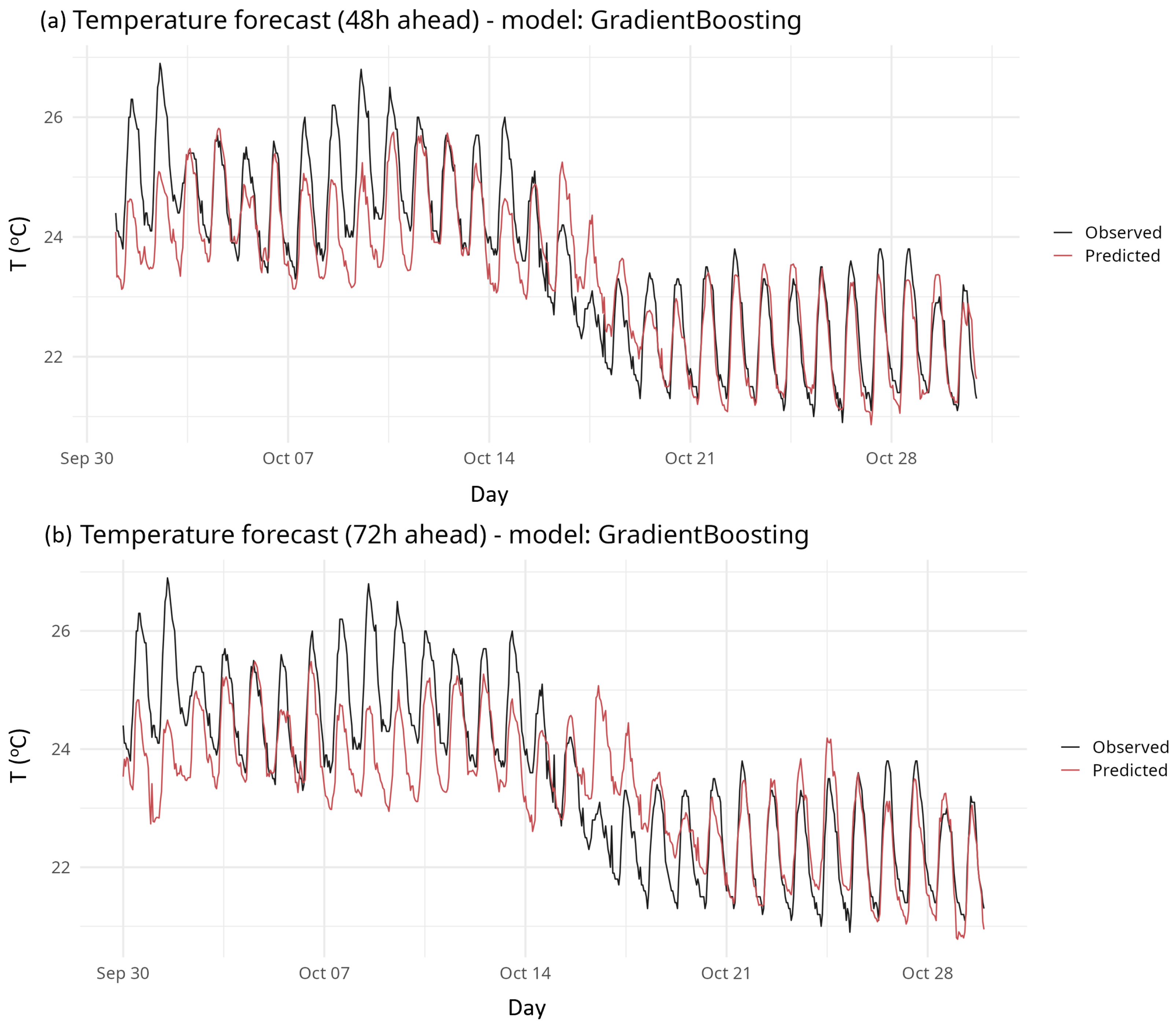
To gain a holistic insight into the model’s performance in reproducing indoor temperature, Figure 5 presents the observed and predicted time series for 48 h and 72 h forecasting horizons for an indicative month (October), rather than the full study period. Overall, the model reproduces the temperature temporal evolution satisfactorily, capturing both the general trend and daily fluctuations. In general, the predictions (red) tend to slightly underestimate the maxima and, in some cases, overestimate the minima. This suggests a mild smoothing effect (regression toward the mean), which is commonly observed in ensemble-based machine learning forecasting models. For both forecasting horizons, the largest deviations are mainly found during the first days of October, which may be related to increased variability of outdoor conditions and changes in the building’s thermal load. Around mid-October, a clear regime change is observed, with a drop in average temperature, where the model follows this transition reasonably well, albeit with a slight lag, demonstrating its ability to adapt to non-stationary conditions. More specifically, for the 48 h time horizon (Figure 5a), very good agreement is observed between predicted and actual values. The model accurately reproduces both the amplitude and the phase of the daily cycles, with only minor deviations. Conversely, for the 72 h horizon (Figure 5b), the performance shows a slight degradation, as expected due to the increased uncertainty associated with longer forecast horizons. Furthermore, the predicted daily temperature range is slightly reduced compared to the observed one, indicating a smoothing behavior. A small time lag in the appearance of peak values (of the order of a few hours) is also evident, which is typical in multi-step forecasting. Nevertheless, even at the 72 h horizon, the model preserves the 24 h periodicity remarkably well, suggesting that it successfully captures the underlying seasonal patterns. However, the model still reproduces the overall dynamics of the system satisfactorily.

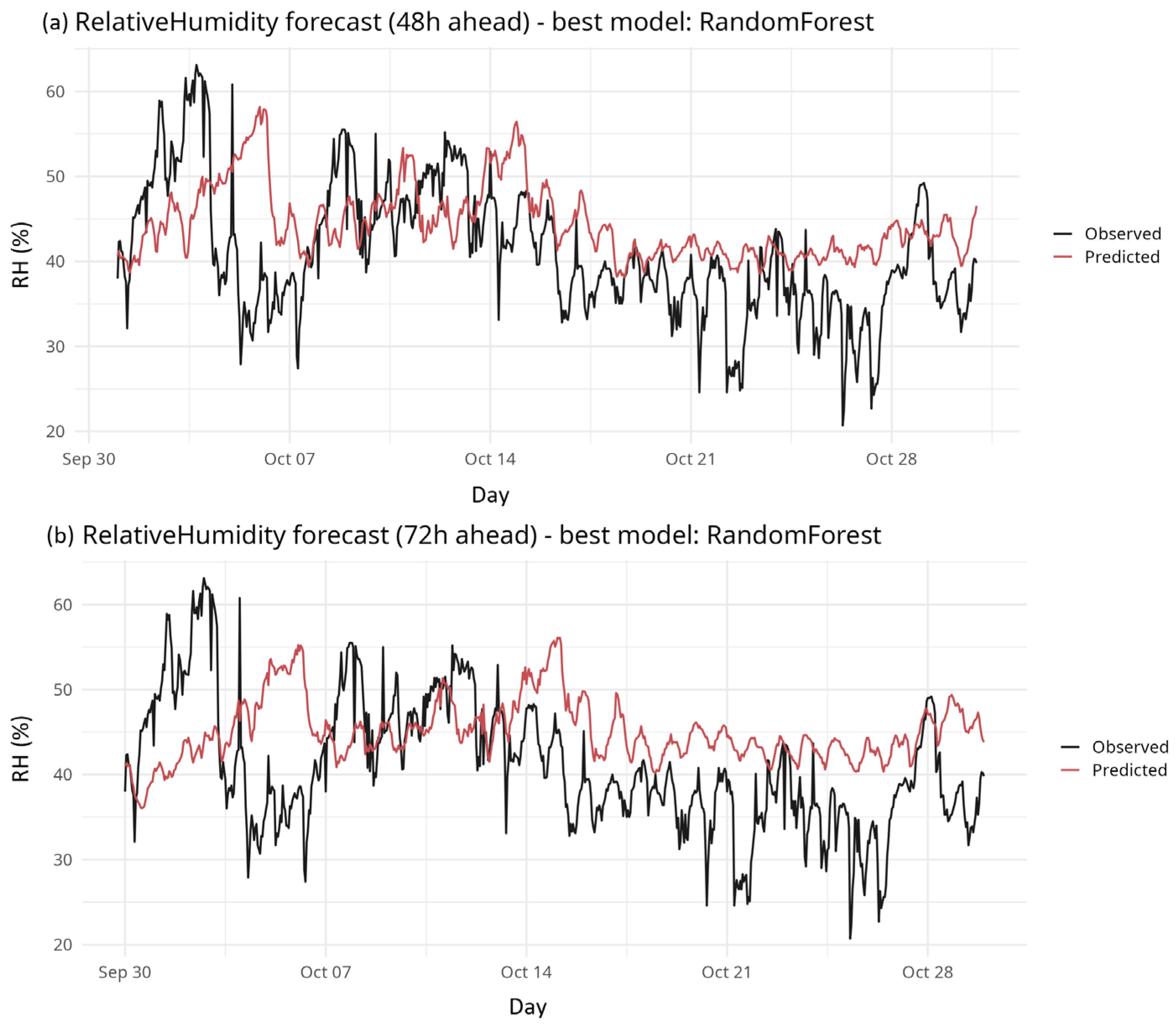
Regarding RH, the model satisfactorily reproduces the general trend; however, it presents significant limitations in capturing short-term variability. More specifically, there is a pronounced smoothing in the forecasts, resulting in a significant underestimation of the range of variation of RH. The model tends to overestimate low values and, in some cases, underestimate high values, which indicates a tendency towards the mean value (regression to the mean). For the 48 h horizon (Figure 6a), although the model follows the general trend, it struggles to capture abrupt changes, such as sharp peaks and troughs. At the same time, for the 72 h horizon (Figure 6b), the performance deteriorates further, with greater smoothing and convergence of the predictions within a narrower range of values. Consequently, the sharp fluctuations and local minima observed in the measurements are not adequately reproduced, highlighting the model’s difficulty in reproducing high short-term variability and abrupt fluctuations. Nevertheless, despite the above limitations, the model retains the ability to reproduce the overall dynamics of relative humidity, which suggests that it has captured the basic patterns of the time series, but has difficulty reproducing the high variability.

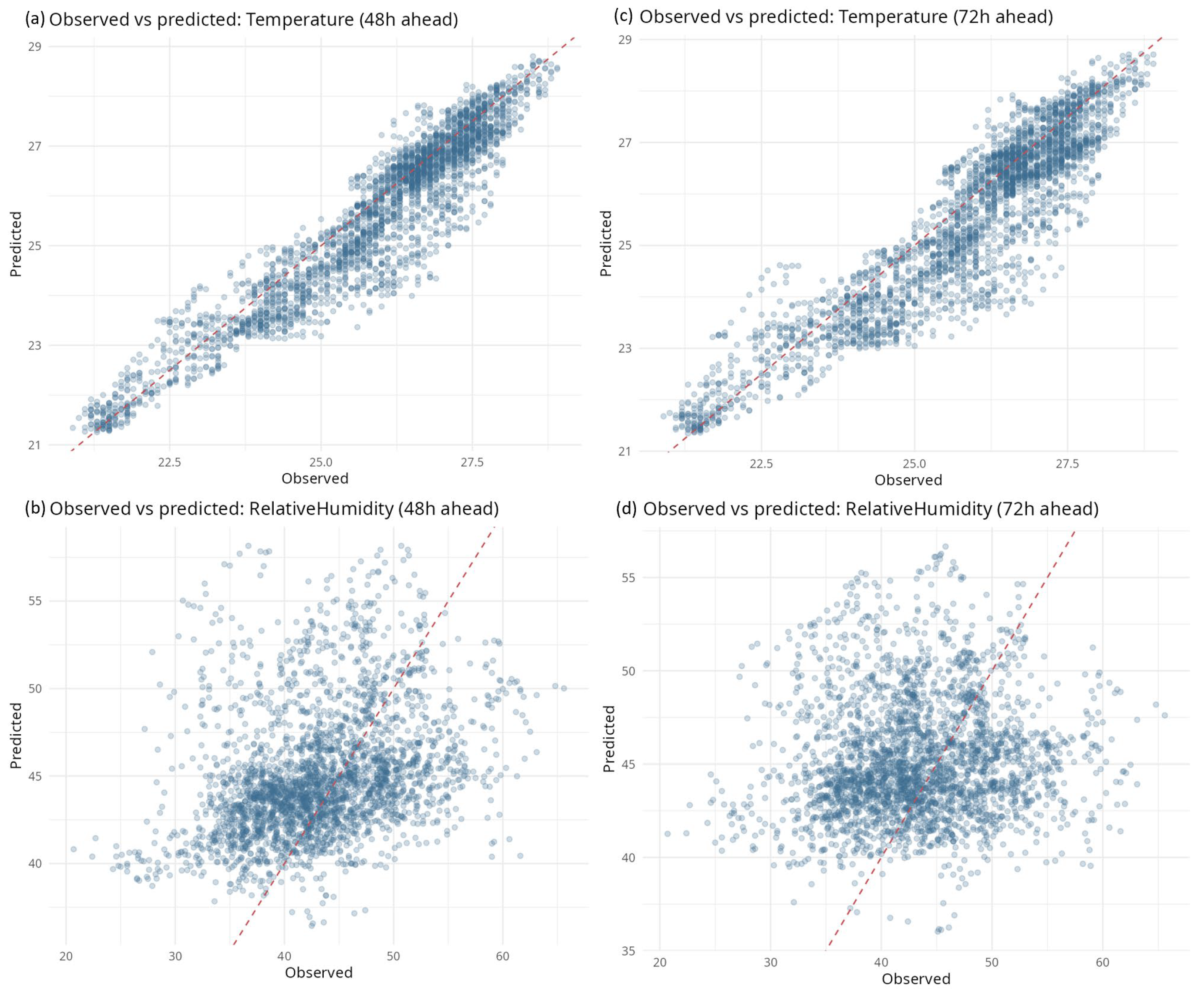
Figure 7 displays scatter plots between observed and predicted values for indoor temperature and RH at 48 and 72 h forecasting horizons. These plots were constructed to visually assess the predictive performance of the models and to identify potential deviations between observed and predicted values. The proximity of the points to the 1:1 line reflects the agreement between predictions and observations, providing insight into the ability of the models to reproduce the indoor microclimate conditions. Specifically, for indoor temperature, the results indicate a strong agreement between observed and predicted values for both forecasting horizons. The majority of points are closely aligned along the 1:1 line, suggesting that the models effectively capture the underlying thermal dynamics of the space. A slight increase in dispersion is observed at the 72 h horizon, indicating a gradual reduction in predictive accuracy with increasing forecast time.

In contrast, the plots for relative humidity reveal a weaker relationship between observed and predicted values. The points are more widely scattered and deviate substantially from the 1:1 line, indicating limited model performance. This pattern suggests that the models tend to approximate average conditions rather than accurately capturing variability and extreme values of relative humidity. These findings highlight a clear contrast in predictive behavior, with temperature being reliably reproduced due to its temporal persistence. In contrast, RH shows weaker agreement, reflecting its more complex and externally driven dynamics.

4. Discussion

Indoor environmental condition prediction is a valuable means of enabling earlier identification of potentially harmful conditions in museums and thus preventing damage to museum collections. In addition to informing how heating/ventilation/air conditioning (HVAC), exhibit space planning, and emergency responses to extreme microclimates are managed, forecasting temperature and RH also allow these systems to be operated efficiently. As such, this study examined which machine learning models were best suited to predicting temperature and relative humidity at the Archaeological Museum of Delphi, using hourly time-series data from both indoor and outdoor environments for two forecast horizons: 48 h and 72 h.

The results showed that indoor temperature was forecast with very good precision over two time periods using the gradient boosting method (48 h: R² = 0.901, RMSE = 0.541; 72 h: R² = 0.849, RMSE = 0.668). Conversely, the predictions of RH showed much lower performance than those of temperature, as even the best model (random forest) yielded a negative R² value at both time periods. This difference has already been highlighted in other studies on the prediction of indoor microclimates, showing that RH is a variable more complex and uncertain than temperature. For instance, Lu and Viljanen [28] reported larger errors and wider prediction intervals for RH, attributing this behavior to the dynamic and unstable nature of the RH system, as well as the possible absence of critical variables from the prediction models.

The differences in forecastable performance for the two variables appear to be related to the physics of the indoor environment. As seen from feature importance and SHAP values, temperature is mostly a function of both the indoor temperature and time-based lagged values of it (temp_in, temp_in_lag1, temp_in_lag24). The building’s strong thermal inertia explains why indoor temperature exhibits a high degree of temporal persistence. On the other hand, RH is more highly influenced by seasonal and outdoor climate variables (e.g., day, sin_day, cos_day; and ERA5 external temperature) and thus exhibits much less temporal persistence than indoor temperature. The relative unpredictability of humidity has been reported in other studies concerning indoor environments. These studies have shown that there exists greater variation both temporally and spatially for RH. According to Zhou et al. [29], the difficulty in predicting indoor humidity stems from its relationship with multiple interacting variables across diverse locations and environmental conditions. Zhou et al. [29] found that even in systems with abundant monitoring data from various sensors, machine learning techniques can improve RH predictions.

The comparison of the models indicates that predictive performance depends on the characteristics of the underlying dataset and the nature of the target variable. Deep learning techniques, particularly recurrent neural networks (RNNs) and long short-term memory (LSTM) models, have also been widely applied in time-series forecasting due to their ability to capture long-term temporal dependencies in sequential data [30,31]. However, Gradient Boosting Machines and Random Forests have demonstrated strong performance in ensemble regression-based models and have been highly successful at forecasting environmental time series [32]. Regarding temperature, the gradient boosting machine consistently produced the highest predictive accuracy, likely because it effectively captures both smooth and nonlinear relationships. Similarly, Ramadan et al. [33] found that indoor temperatures can be predicted with high accuracy using both ensemble and tree-based methods. As a result, these types of predictive models are being considered for use in building control systems. Regarding RH, Random Forest performed better in terms of total predictive ability, although it was still very low. The greater stability/robustness to unstable/noisy input data of RF is most likely the cause of this, because it makes predictions by averaging many independent decision trees. SVR was not identified as the best model in any of the cases analyzed above, and this may be due to its sensitivity to parameter selection and its poor treatment of complex seasonal time series. The overall results indicate that the microclimate variable will affect the type/model used to predict it. Temperature and RH are unique in their temporal characteristics (i.e., time duration), degree of complexity, and sensitivity to other environmental conditions.

To further assess the forecasting merit of the proposed models, baseline performance was evaluated using persistence, weekly seasonal-naïve, and rolling-mean methods. Temperature results indicated that Gradient Boosting was the best-performing model, substantially exceeding both the weekly seasonal-naïve and rolling climatology baseline models. Relative to the weekly seasonal-naïve benchmark, RMSE was reduced by 36.7% for the 48 h forecast horizon and by 21.9% for the 72 h horizon. Nevertheless, persistence remained a particularly strong benchmark for temperature prediction, reflecting the high thermal inertia of the museum building and the strong temporal persistence of indoor temperature conditions.

Regarding RH, the negative R² values indicate that the models did not consistently achieve better performance than the mean reference predictor. However, Random Forest produced a 13.5% improvement over persistence at the 48 h horizon and a 14.3% improvement at the 72 h horizon. These results suggest that the RH models capture some degree of horizon-dependent signal; however, they do not provide sufficient confidence to support general conclusions regarding the reliability of RH forecasts. Their current value is therefore mainly diagnostic, as they highlight limitations in the monitored variables and provide a quantitative benchmark against which future improvements can be assessed.

The relatively weak performance of the RH models is likely related to the absence of several important physical drivers from the available dataset. While the predictors included indoor and outdoor temperature and RH measurements, precipitation, ERA5 variables, and temporal signatures such as lagged values and rolling averages, other relevant factors known to influence indoor moisture dynamics were not available. These include HVAC operational status, door-opening frequency and duration, visitor occupancy patterns, absolute humidity, humidity ratio, and solar loading effects. Temperature can be predicted more successfully because the thermal mass of the building introduces a strong degree of temporal persistence, making future values more dependent on recent conditions. In contrast, RH is more directly influenced by short-term moisture sources and air-exchange processes and therefore exhibits lower predictive stability over time. Future work should focus on collecting these additional variables and on developing more physically based predictors, such as absolute humidity and dew point temperature, in order to improve RH forecasting performance.

Although the framework demonstrates good predictive skill for indoor temperature, the current implementation does not explicitly model threshold exceedance events or conservation-risk classes. Instead, it mainly provides continuous forecasts of indoor environmental conditions that may support preventive decision-making. This study should be seen as an initial step toward developing a forecasting framework for managing museum microclimates. The models were created and tested using data from a single monitoring sensor installed in one gallery of the Archaeological Museum of Delphi. Although the selected gallery was considered representative of the monitored environment, spatial variability within the museum was not assessed in the current study. Future work will focus on expanding the monitoring network to multiple rooms within the museum, as well as to additional heritage buildings, in order to evaluate model transferability, spatial robustness, and general applicability. Furthermore, the framework could be extended toward a more comprehensive early-warning system by integrating conservation thresholds, anomaly detection techniques, and event-based classification approaches.

5. Conclusions

In this study, we developed and evaluated a multi-source, time-aware machine learning framework for predicting indoor temperature and relative humidity at the Archaeological Museum of Delphi, utilizing indoor monitoring data, outdoor meteorological observations, and ERA5 reanalysis data. The proposed framework combined lagged and rolling-window predictors with chronological train/validation/test splitting and rolling-origin cross-validation in order to evaluate predictive performance at 48 h and 72 h forecasting horizons.

The results showed high reliability for temperature prediction, while RH prediction was still a big challenge. Overall, the Gradient Boosting Machine model was the best performer for the prediction of temperature for both time horizons, while the Random Forest model had the best performance for RH, with limited predictive ability. These results showed that the temporal stability and predictability of temperature were higher than those of the relative humidity.

The comparison of machine learning algorithms also revealed that each model is effective for predicting different kinds of variables. Gradient Boosting was found to perform better in modeling the nonlinear but comparatively smooth thermal behavior of the indoor environment, while Random Forest was more robust in modeling the relative humidity, which is comparatively more variable and complex. In all the test cases, the Support Vector Regression model failed to outperform the ensemble-based models. Moreover, indoor temperature conditions and their temporal lags were the most important factors in influencing temperature forecasts, emphasizing the importance of thermal inertia in the building and temporal continuity. The RH predictions, on the contrary, rely more on seasonality indexes and outdoor climate factors, reflecting a higher sensitivity to external environmental factors.

The results from this study can be used by museum conservators, museum conservation management, HVAC operators, and cultural heritage authorities, providing tools for predicting and warning in advance, assessing the environmental risk, and making informed decisions on indoor microclimate management. We plan to continue indoor microclimate monitoring on selected museums and heritage buildings, as well as to further enhance the framework for predicting the occurrence of potentially critical environmental conditions at an early stage. The incorporation of future climate scenarios and more detailed forecasting information can further assist the museum authorities and conservation professionals in safeguarding sensitive cultural heritage collections.

References

1. Johnson, E.V.; Horgan, J.C. Museum Collection Storage; UNESCO: Paris, France, 1979. [Google Scholar]
2. Canadian Conservation Institute. Agents of Deterioration; Canadian Conservation Institute: Ottawa, ON, Canada, 2025. [Google Scholar]
3. Luosujärvi, R.A.; Husman, T.M.; Seuri, M.; Pietikäinen, M.A.; Pollari, P.; Pelkonen, J.; Hujakka, H.T.; Kaipiainen-Seppänen, O.A.; Aho, K. Joint Symptoms and Diseases Associated with Moisture Damage in a Health Center. Clin. Rheumatol. 2003, 22, 381–385. [Google Scholar] [CrossRef] [Scilit] [PubMed]
4. Reijula, K. Moisture-Problem Buildings with Molds Causing Work-Related Diseases. In Advances in Applied Microbiology; Elsevier: Amsterdam, The Netherlands, 2004; Volume 55, pp. 175–189. [Google Scholar]
5. Pretelli, M.; Fabbri, K. (Eds.) Historic Indoor Microclimate of the Heritage Buildings; Springer International Publishing: Cham, Switzerland, 2018; ISBN 978-3-319-60341-4. [Google Scholar]
6. Bernardi, A. Microclimate Inside Cultural Heritage Buildings—Softcover; Casa Editrice Il Prato: Saonara, Italy, 2008. [Google Scholar]
7. Spagnuolo, A.; Vetromile, C.; Masiello, A.; Alberghina, M.F.; Schiavone, S.; Mantile, N.; Di Cicco, M.R.; Solino, G.; Lubritto, C. Protecting Archaeological Collections in Capua Archaeological Museum (Italy): The Importance of Microclimatic Monitoring and Non-Invasive Diagnostic Investigations. Acta IMEKO 2024, 13, 2. [Google Scholar] [CrossRef] [Scilit]
8. Brimblecombe, P.; Bibl, A.; Fischer, C.; Pristacz, H.; Querner, P. Microclimate of the Natural History Museum, Vienna. Heritage 2025, 8, 124. [Google Scholar] [CrossRef] [Scilit]
9. Faubel, C.; Arvanitidis, A.I.; Iskandar, L.; Martinez-Molina, A.; Alamaniotis, M. Comparative Analysis of Artificial Intelligence Models for Real-Time and Future Forecasting of Environmental Conditions: A Wood-Frame Historic Building Case Study. J. Build. Eng. 2024, 98, 111474. [Google Scholar] [CrossRef] [Scilit]
10. ISO 11799:2015; Information and Documentation—Document Storage Requirements for Archive and Library Materials. International Organization for Standardization: Geneva, Switzerland, 2015.
11. EN 16893:2018; Conservation of Cultural Heritage—Specifications for Location, Construction, and Modification of Buildings or Rooms Intended for the Storage or Use of Heritage Collections. European Committee for Standardization (CEN): Brussels, Belgium, 2018.
12. ASHRAE. Museums, Galleries, Archives, and Libraries; ASHRAE: Atlanta, GA, USA, 2019. [Google Scholar]
13. Boesgaard, C.; Hansen, B.V.; Kejser, U.B.; Mollerup, S.H.; Ryhl-Svendsen, M.; Torp-Smith, N. Prediction of the Indoor Climate in Cultural Heritage Buildings through Machine Learning: First Results from Two Field Tests. Herit. Sci. 2022, 10, 176. [Google Scholar] [CrossRef] [Scilit]
14. Zannis, G.; Santamouris, M.; Geros, V.; Karatasou, S.; Pavlou, K.; Assimakopoulos, M.N. Energy Efficiency in Retrofitted and New Museum Buildings in Europe. Int. J. Sustain. Energy 2006, 25, 199–213. [Google Scholar] [CrossRef] [Scilit]
15. Fabbri, R.; Gabrielli, L.; Ruggeri, A.G. Interactions between Restoration and Financial Analysis: The Case of Cuneo War Wounded House. J. Cult. Herit. Manag. Sustain. Dev. 2018, 8, 145–161. [Google Scholar] [CrossRef] [Scilit]
16. Mitchell, T.M. Machine Learning; McGraw-Hill series in Computer Science; McGraw-Hill: New York, NY, USA, 2013. [Google Scholar]
17. Kobayashi, K.; Hwang, S.-W.; Okochi, T.; Lee, W.-H.; Sugiyama, J. Non-Destructive Method for Wood Identification Using Conventional X-Ray Computed Tomography Data. J. Cult. Herit. 2019, 38, 88–93. [Google Scholar] [CrossRef] [Scilit]
18. Lu, Z.; Wang, W.; Guo, T.; Li, Y.; Wang, F. Decoding Urban Policies: NLP-Driven Concise Explanations. Environ. Plan. B Urban Anal. City Sci. 2026, 53, 125–142. [Google Scholar] [CrossRef] [Scilit]
19. Pei, J.; Gong, J.; Wang, Z. Risk Prediction of Household Mite Infestation Based on Machine Learning. Build. Environ. 2020, 183, 107154. [Google Scholar] [CrossRef] [Scilit]
20. Alawadi, S.; Mera, D.; Fernández-Delgado, M.; Alkhabbas, F.; Olsson, C.M.; Davidsson, P. A Comparison of Machine Learning Algorithms for Forecasting Indoor Temperature in Smart Buildings. Energy Syst. 2022, 13, 689–705. [Google Scholar] [CrossRef] [Scilit]
21. Cheng, C.-C.; Lee, D. Artificial Intelligence-Assisted Heating Ventilation and Air Conditioning Control and the Unmet Demand for Sensors: Part 1. Problem Formulation and the Hypothesis. Sensors 2019, 19, 1131. [Google Scholar] [CrossRef] [Scilit] [PubMed]
22. Boeri, A.; Fabbri, K.; Longo, D.; Roversi, R. Indoor Microclimate Monitoring in Heritage Buildings: The Bologna University Library Case Study. Buildings 2025, 15, 3235. [Google Scholar] [CrossRef] [Scilit]
23. Lagouvardos, K.; Kotroni, V.; Bezes, A.; Koletsis, I.; Kopania, T.; Lykoudis, S.; Mazarakis, N.; Papagiannaki, K.; Vougioukas, S. The Automatic Weather Stations NOANN Network of the National Observatory of Athens: Operation and Database. Geosci. Data J. 2017, 4, 4–16. [Google Scholar] [CrossRef] [Scilit]
24. Tringa, E.; Kavroudakis, D.; Tolika, K. Microclimate-Monitoring: Examining the Indoor Environment of Greek Museums and Historical Buildings in the Face of Climate Change. Heritage 2024, 7, 1400–1418. [Google Scholar] [CrossRef] [Scilit]
25. Breiman, L. Random Forests. Mach. Learn. 2001, 45, 5–32. [Google Scholar] [CrossRef] [Scilit]
26. Friedman, J.H. Greedy Function Approximation: A Gradient Boosting Machine. Ann. Stat. 2001, 29, 1189–1232. [Google Scholar] [CrossRef] [Scilit]
27. Cortes, C.; Vapnik, V. Support-Vector Networks. Mach. Learn. 1995, 20, 273–297. [Google Scholar] [CrossRef] [Scilit]
28. Lu, T.; Viljanen, M. Prediction of Indoor Temperature and Relative Humidity Using Neural Network Models: Model Comparison. Neural Comput. Appl. 2009, 18, 345–357. [Google Scholar] [CrossRef] [Scilit]
29. Zhou, X.; Guo, Q.; Han, J.; Wang, J.; Lu, Y.; Shi, J.; Kou, M. Real-Time Prediction of Indoor Humidity with Limited Sensors Using Cross-Sample Learning. Build. Environ. 2022, 215, 108964. [Google Scholar] [CrossRef] [Scilit]
30. Hochreiter, S.; Schmidhuber, J. Long Short-Term Memory. Neural Comput. 1997, 9, 1735–1780. [Google Scholar] [CrossRef] [Scilit] [PubMed]
31. Lim, B.; Zohren, S. Time-Series Forecasting with Deep Learning: A Survey. Phil. Trans. R. Soc. A 2021, 379, 20200209. [Google Scholar] [CrossRef] [Scilit] [PubMed]
32. Effrosynidis, D.; Spiliotis, E.; Sylaios, G.; Arampatzis, A. Time Series and Regression Methods for Univariate Environmental Forecasting: An Empirical Evaluation. Sci. Total Environ. 2023, 875, 162580. [Google Scholar] [CrossRef] [Scilit] [PubMed]
33. Ramadan, L.; Shahrour, I.; Mroueh, H.; Chehade, F.H. Use of Machine Learning Methods for Indoor Temperature Forecasting. Future Internet 2021, 13, 242. [Google Scholar] [CrossRef] [Scilit]
Figure 1. Conceptual framework of the ML-based indoor microclimate forecasting and early-warning system, showing monitoring, forecasting, interpretability, and preventive conservation actions.
Applsci 16 06092 g001
Figure 2. Geographic context of the study area: (a) regional map of Greece indicating the location of Delphi; (b) satellite view of the Archaeological Museum of Delphi and its immediate surroundings. Base map and satellite imagery: Google Earth Pro.
Applsci 16 06092 g002
Figure 3. Floor plan of the Archaeological Museum of Delphi. The red box highlights the study area (Gallery I).
Applsci 16 06092 g003
Figure 4. Machine learning workflow for model development and reproducibility, including data preprocessing, feature engineering, train/validation/test splitting, model training, evaluation, and interpretation.
Applsci 16 06092 g004
Figure 5. Time series of observed and predicted indoor temperature for (a) 48 h and (b) 72 h forecasting horizons using the best-performing model (Gradient Boosting). Results are shown for an indicative month (October), rather than the full study period. The comparison illustrates the model’s ability to capture both short-term variability and overall temporal trends.
Applsci 16 06092 g005
Figure 6. Time series of observed and predicted indoor RH for (a) 48 h and (b) 72 h forecasting horizons using the best-performing model (Random Forest). Results are shown for an indicative month (October), rather than the full study period. The comparison illustrates the model’s ability to capture both short-term variability and overall temporal trends.
Applsci 16 06092 g006
Figure 7. Scatter plots between observed and predicted values of indoor temperature (a,c) and RH (b,d) for 48 h and 72 h forecasting horizons. The dashed red line represents the 1:1 agreement, highlighting model performance and deviations from perfect prediction.
Applsci 16 06092 g007