Construction of a Continuous High-Resolution PWV Using GNSS/ERA5, InSAR, and FY-4A Data: A Case Study of the Jiaodong Peninsula and Adjacent Seas

Featured Application

We established a multi-source fusion framework for high-resolution and sea–land continuous PWV monitoring in the Jiaodong Peninsula and adjacent seas. This study is particularly valuable for coastal moisture monitoring and precipitation-related meteorological applications.

Abstract

Precipitable water vapor (PWV) is a pivotal parameter in the measurement of atmospheric water vapor content. Interferometric Synthetic Aperture Radar (InSAR) is capable of retrieving PWV with high accuracy and spatial resolution. However, the limitations imposed by factors such as low coherence and phase distortion prevent the monitoring of PWV over the sea surface by InSAR. For this problem, a joint InSAR/Fengyun sea–land cooperative PWV construction method is proposed using constraints from the Global Navigation Satellite System (GNSS) and ERA5 reanalysis data. The Jiaodong Peninsula of China was selected as the research area. The PWV over the land of the Jiaodong Peninsula was obtained by GNSS/ERA5/InSAR. The PWV over the nearby sea was obtained by Fengyun-4A (FY-4A). The PWV reconstruction over the sea and land region is realized by means of unified reference correction and transition processing. The results indicate that InSAR PWV and FY-4A PWV show good agreement with GNSS PWV, with R², MAE and RMSE values of 0.955, 1.86 mm and 2.32 mm for InSAR PWV, and 0.961, 1.90 mm and 2.28 mm for FY-4A PWV, respectively. The fused PWV significantly improves spatial completeness while preserving fine spatial structures, with an annual PWV range of 0.35–59.74 mm and a clear seasonal cycle from 4.16 mm in winter to 33.24 mm in summer. The results effectively capture the coastal moisture transition, with the strongest PWV gradient reaching 0.823 mm/km in the 0–10 km coastal zone during the warm season. PWV also shows the strongest correlation with dew point, with a Spearman correlation coefficient of 0.94. This study overcomes the limitation that PWV is restricted to land areas and provides reliable data support for the analysis of water vapor structures in coastal regions.

1. Introduction

The coastal zone is of significant to the global economy, culture and human life. The prevailing weather conditions in the coastal zone exert a significant influence on human activities. The presence and progression of severe weather conditions are influenced by atmospheric water vapor content [1]. Precipitable water vapor (PWV) is defined as the total amount of liquid water contained within a unit area of the atmospheric column, extending from the surface to the tropopause. PWV effectively reflects the transport pathways, convergence processes, and spatio-temporal distribution characteristics of atmospheric water vapor [2]. In the context of sea–land transition zones, PWV frequently manifests pronounced spatial gradients and heterogeneous distribution patterns. This phenomenon is attributable to thermal variations between the ocean and the land, in conjunction with disparities in water vapor transport pathways. In order to elucidate the characteristics of water vapor structures in coastal regions and their influence on heavy precipitation processes, it is imperative to construct a spatially continuous PWV with high spatial resolution.

Recent advancements in satellite remote sensing and ground-based observation technologies have facilitated the development of diverse methodologies for the retrieval of PWV [3]. The Global Navigation Satellite System (GNSS) offers the advantage of conducting all-weather continuous observations and can provide highly accurate, stable, and reliable PWV estimates [4,5]. Nevertheless, the findings are constrained by the spatial distribution density of stations as PWV can only be ascertained at discrete locations. Reanalysis products represented by European Centre for Medium-Range Weather Forecasts (ECMWF) Reanalysis v5 (ERA5) data provide spatially continuous and temporally consistent water vapor information at regional to global scales [6]. ERA5 PWV has been shown to benefit from the assimilation of multi-source observations and numerical weather prediction models, exhibiting good overall stability and completeness. This model is extensively used in the field of atmospheric water vapor studies. Nonetheless, the instrument’s comparatively coarse spatial resolution imposes constraints on its capacity to discern fine-scale spatial variability and local structural intricacies of water vapor. Interferometric Synthetic Aperture Radar (InSAR) has the capacity to conduct large-scale ground observations under all-time and all-weather conditions. Furthermore, the InSAR technique can resolve atmospheric delay structures at high spatial resolution, thereby revealing the intricate spatial heterogeneity of water vapor [7]. This renders it well suited for the retrieval of detailed water vapor over land areas. However, due to low coherence and phase distortion, it is challenging to obtain reliable information over ocean regions. The Fengyun-4A (FY-4A) meteorological satellite, independently developed by China, has the capacity to provide PWV information with continuous coverage over both land and ocean. Nonetheless, the spatial resolution and the capacity to characterize local structural details are comparatively restricted [8]. These discrepancies suggest that a solitary data source is inadequate in meeting the combined requirements of high accuracy, high spatial resolution, and continuous sea–land coverage. Consequently, multi-source data fusion has gradually become an important approach for constructing high-quality PWV. The integration of the complementary advantages of different datasets is expected to enhance the completeness and reliability of regional water vapor. The multi-source fusion strategy set out in this study is fundamentally a partitioned collaborative reconstruction method based on the spatial applicability of different datasets, as opposed to a traditional pixel-level weighted fusion approach.

The incorporation of GNSS PWV and ERA5 PWV for constraint and consistency correction enables InSAR PWV to preserve detailed spatial features while concomitantly improving overall accuracy, stability, and reliability. Previous studies have shown that the combination of InSAR with GNSS observations and ERA5 reanalysis data constitutes an effective way to retrieve high-resolution PWV. Since the initial proposal of InSAR for PWV retrieval by Tarayre et al. (1996) [9], numerous studies have concentrated on converting InSAR-derived differential PWV into absolute PWV through GNSS and ERA5 constraints, thereby reducing systematic bias and enhancing retrieval performance [10,11,12,13,14]. The findings of these studies demonstrate the considerable capability of InSAR for high-resolution PWV retrieval. However, the InSAR technique is contingent upon stable surface scatterers in order to maintain interferometric coherence. Conversely, the dynamic behavior of the ocean surface precludes the formation of persistent scatterers, thus resulting in significant coherence loss over marine areas [15,16,17]. Consequently, existing InSAR-derived PWV products are generally limited to land areas, leaving substantial gaps over the ocean and restricting analyses of cross-shore PWV gradients and sea–land interaction processes.

In the context of oceanic regions, the InSAR technique is unable to provide reliable atmospheric delay information due to the low coherence of the sea surface, which results in persistent gaps in near-shore and offshore water vapor. In order to compensate for this limitation, the introduction of FY-4A PWV is recommended, with the aim of providing continuous water vapor information over the ocean. The extension of the PWV from land to adjacent seas would be enabled by this measure, and would support sea–land integrated reconstruction. Previous studies have demonstrated that FY-4A PWV has good consistency with GNSS-derived PWV and its accuracy can be further improved through regional calibration and model optimization [18,19,20,21,22]. These efforts confirm the strong potential of FY-4A for continuous PWV monitoring over both land and ocean, particularly in marine regions where ground-based observations are sparse. However, the spatial resolution of FY-4A PWV is relatively coarse, and its capability to characterize fine-scale water vapor structures is still limited.

Despite recent progress in PWV retrieval, most fusion-based studies have mainly focused on terrestrial regions, and the construction of spatially continuous PWV across coastal land–sea transition zones remain insufficiently addressed. InSAR can provide high-resolution PWV information over land, but it cannot provide reliable PWV over ocean regions because of low coherence and phase distortion. FY-4A PWV provides continuous coverage over both land and ocean, but its relatively coarse spatial resolution limits its ability to resolve fine-scale coastal and topographic water vapor structures. GNSS and ERA5 data can provide useful constraints for calibration and consistency correction, but they cannot independently provide a high-resolution and spatially continuous sea–land PWV field. Thus, the key methodological gap lies in how to preserve the high-resolution spatial details of InSAR over land, introduce continuous FY-4A PWV information over the ocean, and achieve a physically reasonable transition across the coastline.

Therefore, achieving a spatially continuous sea–land PWV while retaining the high-resolution benefits of InSAR has become a major focus in coastal atmospheric water vapor research. To address this gap, this study proposes a sea–land partitioned collaborative PWV reconstruction framework for the Jiaodong Peninsula and adjacent seas. In this framework, GNSS- and ERA5-derived PWV are used to constrain and calibrate InSAR-derived PWV over land, where InSAR provides the primary high-resolution water vapor information. Over ocean regions, FY-4A PWV is introduced to mitigate the lack of reliable InSAR observations and to provide continuous marine coverage. A coastal transition treatment is then applied to connect the land-dominated InSAR PWV and ocean-dominated FY-4A PWV into a spatially continuous sea–land PWV field. Therefore, the main contribution of this study lies in constructing a coastal partitioned PWV reconstruction strategy rather than a general pixel-level fusion algorithm. The proposed framework is applied to the Jiaodong Peninsula and adjacent seas to investigate the spatial continuity, coastal gradients, and seasonal variation of PWV in a typical coastal region.

2. Materials and Methods

2.1. Region and Data

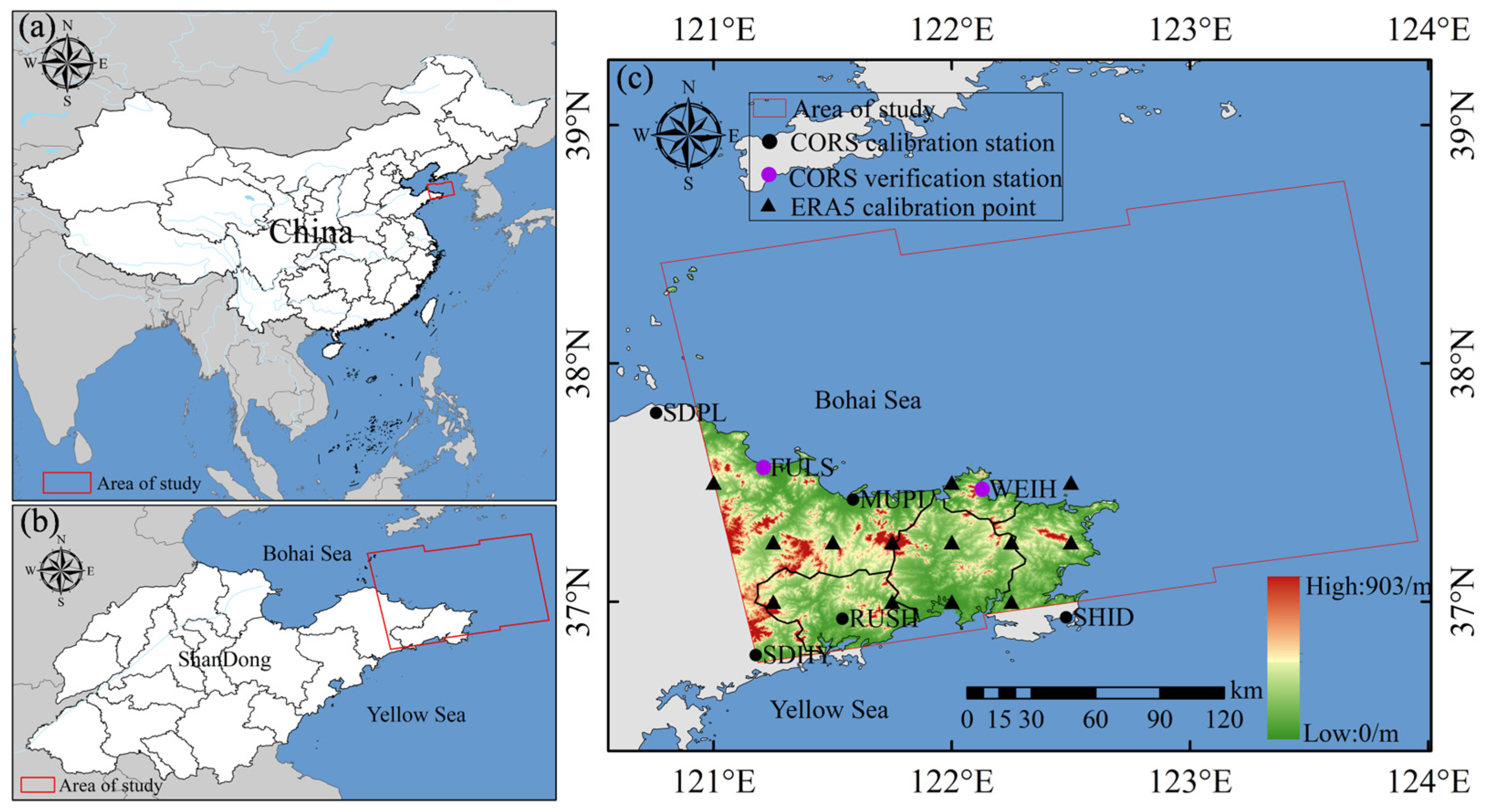
The geographical area selected for this study is the coastal region of the Jiaodong Peninsula and adjacent seas, as illustrated in Figure 1. The geographical extent of the study area is approximately 120.5–124° E and 36.5–38.5° N. This region is situated in the mid-latitude zone of China’s eastern coast, bounded by the Yellow Sea to the east and the Bohai Sea to the north, representing a typical sea–land transition zone. The region is distinguished by a marked interpenetration of land and sea, a diversity of terrain types, and a coastline with numerous indentations. These geographical features give rise to distinctive geomorphic structures and thermal distribution patterns. The repeated exchange of heat and moisture between the ocean and the land gives rise to a highly heterogeneous and complex spatio-temporal distribution of atmospheric water vapor in this region.

Multi-temporal Sentinel-1A IW mode SLC data covering the study area in 2022 were selected as the data source for InSAR processing. Furthermore, the ERA5 PWV data and FY-4A PWV data were utilized. Sentinel-1A data were obtained from the European Space Agency (ESA) website (https://search.asf.alaska.edu/). ERA5 data can be obtained from the European Centre for Medium-Range Weather Forecasts (https://www.ecmwf.int) and encompasses meteorological variables pertaining to atmospheric precipitable water, surface temperature, and water vapor pressure. FY-4A PWV data are available from the National Satellite Meteorological Center (https://satellite.nsmc.org.cn/).

GNSS PWV data were derived from observations collected at seven Continuously Operating Reference Stations (CORS) provided by the Shandong Institute of Land Surveying and Mapping and processed using GAMIT 10.76. GAMIT is a scientific GNSS data processing software package that can be used for high-precision positioning, baseline processing, and estimation of zenith tropospheric delay, which provides the basis for subsequent PWV retrieval. The detailed processing strategy is presented in

Table 1. Processing strategy for PWV retrieval using GAMIT 10.76.

Parameters	Handling Strategy
Track processing mode	BASELINE
Type of observed frequency band	LC_AUTCLN
Mapping function model	VMF1
Global tide-free atmospheric load parameter grid file	atml.grid
Sampling interval	30 s
Satellite cutoff altitude Angle	10°
Meteorological parameters	GPT50
The static delay model of the zenith	Saastamoinen
Global atmospheric tidal grid model file	atl.grid

. In this study, GNSS PWV, in combination with PWV from selected ERA5 grid points, was utilized for the calibration of the InSAR differential precipitable water vapor (ΔPWV). The GNSS PWV data were derived from the observation data of seven CORS provided by the Shandong Institute of Land Surveying and Mapping. As illustrated in Figure 1, the geographical locations of the seven CORS and the 13 ERA5 grid points in and around the study area are delineated. It is worth noting that FULS and WEIH stations do not participate in the calibration process as independent verification points.

2.2. Principle of Research

2.2.1. Principle of Atmospheric Water Vapor Retrieval Using GNSS

During the retrieval of PWV using GNSS [23,24], observations are typically processed using precise point positioning or relative positioning to obtain the zenith total tropospheric delay (ZTD). ZTD is usually composed of the zenith hydrostatic delay (ZHD) and the zenith wet delay (ZWD) [25], as shown in Equation (1):

$$ZWD=ZTD-ZHD$$

(1)

where ZTD, ZHD and ZWD are length quantities and are expressed in millimeter (mm) in the calculation. ZHD can be determined using empirical models such as the Saastamoinen model [26,27], as shown in Equation (2):

$$\mathit{ZHD}={\displaystyle \frac{(2.2767\pm 0.0024)P_s}{1-0.00266\mathit{cos}\left(2\lambda \right)-0.00028H}}$$

(2)

where P_s denotes the surface air pressure (hPa), λ denotes the latitude (rad), and H denotes the station elevation (km).

Subsequently, ZWD [28,29] can be converted into PWV using the conversion factor K, as shown in Equations (3) and (4):

$$PWV=K·ZWD$$

(3)

$$K={\displaystyle \frac{1\times {10}^6}{\rho R_v\left[\left(\frac{k_3}{T_m}\right)+k_2^{\prime }\right]}}$$

(4)

where $T_m$ denotes the weighted mean temperature, $K$ denotes the water vapor conversion factor, depends on $T_m; \rho$ denotes the density of liquid water, $\rho =10^3(\mathrm{k}\mathrm{g}\cdot {\mathrm{m}}^{-3}),R_v$ denotes the specific gas constant of water vapor, $R_v=461.495\left(\mathrm{J}·\mathrm{K}·{\mathrm{k}\mathrm{g}}^{-1}\right),k_2^{\prime },k_3$ represent the atmospheric refractive index constant, $k_2^{\prime }=0.233\left(\mathrm{K}\cdot \mathrm{P}{\mathrm{a}}^{-1}\right),k_3=3.776\times 10^3({\mathrm{K}}^2\cdot \mathrm{P}{\mathrm{a}}^{-1})$.

$T_m$ is the key parameter to convert ZWD into PWV [30], and the accurate expression of its calculation model is of great significance for GNSS technology to detect water vapor [31,32]. $T_m$ is calculated as shown in Equation (5):

$$T_m={\displaystyle \frac{{\int }_h^{\infty }\left(e/T\right)dh}{{\int }_h^{\infty }\left(e/T^2\right)dh}}$$

(5)

where e denotes the water vapor pressure (hPa); T denotes the air temperature (K); h denotes the elevation (m), and the distributions of e and T vary over time and space. The calculation of e is shown in Equation (6):

$$e=E{\displaystyle \frac{R_e}{100}}$$

(6)

where E denotes saturated vapor partial pressure and R_e denotes relative humidity.

2.2.2. Principle of Atmospheric Water Vapor Retrieval Using InSAR

The differential interferometric phase of InSAR consists of deformation phase, topographic phase, atmospheric delay phase, orbital error phase, and noise phase [15], as shown in Equation (7):

$${\varphi }_{i,j}={\varphi }_{\mathit{defo}}^{i,j}+{\varphi }_{\mathit{atm}}^{i,j}+{\varphi }_{\mathit{orb}}^{i,j}+{\varphi }_{\mathit{dem}}^{i,j}+{\varphi }_{\mathit{noise}}^{i,j}$$

(7)

where ${\varphi }_{i,j}$ denotes the differential phase corresponding to the ith pixel of the JTH interferogram; ${\varphi }_{\mathit{defo}}^{i,j}$ denotes the surface deformation in the radar line of sight direction; ${\varphi }_{\mathit{atm}}^{i,j}$ denotes the atmospheric delay phase in the radar line of sight direction; ${\varphi }_{\mathit{orb}}^{i,j}$ denotes the orbital error phase; ${\varphi }_{\mathit{dem}}^{i,j}$ denotes the topographic phase error; and ${\varphi }_{\mathit{noise}}^{i,j}$ denotes the noise phase caused by an imprecise reference Digital Elevation Model (DEM), variations in scattering properties, system thermal noise, and registration errors.

The terrain phase [33] can be removed using the Shuttle Radar Topography Mission Digital Elevation Model (SRTM-DEM), and satellite orbit errors can be corrected with precise orbit ephemerides (POD). Deformation and noise can be further separated through time-series analysis or filtering, leaving only the tropospheric and ionospheric delay phases. In mid- and low-latitude regions, the ionospheric delay of C-band radar signals is negligible in the interferogram; therefore, the atmospheric delay in the InSAR interferogram is primarily attributed to the tropospheric delay (${\varphi }_{\mathit{trop}}$).

The tropospheric delay phase consists of the hydrostatic delay phase, the wet delay phase, and the liquid water delay phase. Under most weather conditions, the delay caused by liquid water is less than 1 mm and can be neglected. Therefore, the tropospheric delay includes only the hydrostatic and wet components [10], as shown in Equation (8):

$${\varphi }_{\mathit{trop}}={\varphi }_{\mathit{ZH}}+{\varphi }_{\mathit{ZW}}$$

(8)

where ${\varphi }_{\mathit{trop}}$ denotes the tropospheric delay phase in the radar line of sight direction; ${\varphi }_{\mathit{ZH}}$ denotes the hydrostatic delay phase; ${\varphi }_{\mathit{ZW}}$ denotes the tropospheric wet delay phase. The tropospheric static delay (${\varphi }_{\mathit{ZH}}$) can be calculated using atmospheric parameters as shown in Equation (9):

$${\varphi }_{\mathit{ZH}}=-{\displaystyle \frac{4\pi \times 10^{-6}}{\lambda \mathit{cos}\theta }}\left[{\displaystyle \frac{K_1\times R}{g\times M_d}}\times \left(P_{\mathit{t}1}-P_{\mathit{t}0}\right)\right]$$

(9)

where ${\varphi }_{\mathit{ZH}}$ denotes the hydrostatic delay phase;$\lambda$ denotes the wavelength of the radar signal (m); $\theta$ denotes the incidence angle of the radar signal; K₁ = 0.776 K·Pa⁻¹, a physical quantity related to refraction; R denotes the universal exponent of ideal gas, R = 8.31434 J/(mol·K); g denotes the acceleration of gravity (m·s⁻²); M_d denotes the molar mass of dry air; $P_{\mathit{t}1}$ denotes the surface pressure at the imaging time of the auxiliary image; and $P_{\mathrm{t}0}$ denotes the surface pressure at the time of main image imaging.

The static delay phase corresponding to each pixel in the interferogram was calculated based on the ERA5 pressure data [34]. The tropospheric wet delay phase was then obtained by subtracting the hydrostatic delay phase from the total tropospheric delay, according to Equation (8). The three delay phases obtained above are all along the satellite line of sight and are expressed in radians. It is necessary to convert the tropospheric delay phase from the line-of-sight direction to the zenith direction, as shown in Equation (10):

$$Z_{td}=-{\displaystyle \frac{\lambda \mathit{cos}\theta }{4\pi }}{\varphi }_{\mathrm{Z}}$$

(10)

where $Z_{td}$ denotes ZTD, ZHD and ZWD in the zenith direction; ${\varphi }_{\mathrm{Z}}$ denotes the corresponding ${\varphi }_{\mathrm{trop}},{\varphi }_{\mathrm{ZH}}$ and ${\varphi }_{\mathrm{ZW}}$. Finally, the conversion factor K is multiplied to convert ZWD to PWV.

To construct a spatial distribution model of T_m applicable to the entire study area, ERA5 data such as temperature, relative humidity [35,36,37], and geopotential were used to compute its spatial distribution. Since ERA5 provides layered data [38,39], T_m is calculated using a summation approach as an approximation of the integral, as shown in Equation (11):

$$T_m={\displaystyle \frac{{\displaystyle {\sum }_{i=0}^{i=n-1}}\frac{e_i}{T_i}\left(h_{i+1}-h_i\right)}{{\displaystyle {\sum }_{i=0}^{i=n-1}}\frac{e_i}{T_i^2}\left(h_{i+1}-h_i\right)}}$$

(11)

where e_i and T_m denote the mean value of vapor pressure and the mean value of absolute temperature from layer i to layer i + 1, respectively, and h denotes the elevation. The weighted average temperature model of the study area constructed according to Equation (11) is put into Equation (4) to calculate the conversion coefficient K, and then Equation (3) is used to obtain the PWV.

GNSS PWV represents the integrated atmospheric water vapor within a conical spatial region centered on the CORS station, as determined by the geometry of satellite signal propagation. Following the treatment commonly adopted in previous studies [16,17,40], and under the assumption that the atmospheric water vapor field around the station is horizontally isotropic, GNSS PWV can be approximated as the mean value of the InSAR-derived differential PWV within a circular neighborhood centered at the GNSS receiver. It should be noted that this approximation assumes a horizontally isotropic water vapor field around the GNSS station. In coastal regions with strong land–sea humidity gradients, this assumption may introduce additional uncertainty into the matching between GNSS PWV and InSAR PWV.

The spatial calibration of InSAR ΔPWV was performed using GNSS PWV and ERA5 PWV. Assuming that a bias constant γ exists between the InSAR ΔPWV and the spatially calibrated InSAR ΔPWVc, the constant γ can be estimated by minimizing the following cost function, as expressed in Equation (12):

$${J\left(\gamma \right)={\sum }_{k=1}^{N_{ERA5+GNSS}}\left\{{∆PWV}_k^{ERA5/GNSS}-{\displaystyle \frac{1}{N_p\left(k\right)}}{\sum }_{i=1}^{N_p\left(k\right)}{∆PWV}_i^{InSAR}+\gamma \right\}}^2$$

(12)

where $J\left(\gamma \right)$ denotes the minimization cost function of γ; $N_{ERA5+GNSS}$ denotes the number of CORS and ERA5 grid points; $N_p\left(k\right)$ denotes the number of InSAR pixels contained within the circular neighborhood centered at the kth CORS station or within the kth ERA5 grid point; ${∆PWV}_k^{ERA5/GNSS}$ denotes the difference in GNSS PWV or ERA5 PWV between InSAR primary image and secondary image at imaging time; ${∆PWV}_i^{InSAR}$ denotes the relative value of PWV retrieved by InSAR. After InSAR ΔPWV is added with the constant γ retrieved from Equation (12), the spatial dimension calibrated InSAR ΔPWVc can be obtained.

2.2.3. Principle of Sea–Land Continuous PWV Fusion

Before sea–land fusion, FY-4A PWV was first adjusted through spatial resampling and Kalman filtering [41,42] to match the spatial grid of InSAR PWV. The final grid resolution was set to 0.00083° × 0.00083°. Kalman filtering was applied only in the FY-4A PWV adjustment stage to improve spatial consistency after resampling, rather than as a post-processing step for the final fused PWV product, as expressed in Equation (13):

$$F_k=F_k^{-}+{\displaystyle \frac{P_k^{-}}{P_k^{-}+R}}\left(Z_k-F_k^{-}\right)=P_k^{-}=F_k^{-}+{\displaystyle \frac{P_{k-1}+Q}{P_k^{-}+R}}\left(Z_k-F_k^{-}\right)$$

(13)

where $F_k^{-}$ and $F_k$ denote the prior and updated FY-4A PWV estimates, respectively; $Z_k$ denotes the resampled FY-4A PWV observation; $P_k^{-}$ denotes the predicted error covariance; Q denotes the process noise variance; and R denotes the observation noise variance. In this study, Q and R were kept constant for all acquisition dates.

For the subsequent sea–land fusion, valid InSAR PWV pixels were directly retained over land to preserve high-resolution spatial details. For ocean pixels, the adjusted FY-4A PWV was used as the primary background field, while an InSAR-derived extrapolated field was introduced as a weak spatial constraint to improve the continuity of the land–sea transition. Specifically, valid InSAR PWV pixels were first extrapolated to ocean pixels using inverse distance weighting [43], and the extrapolated field was then spatially smoothed. Thus, ocean pixels closer to the valid InSAR coverage were assigned a stronger InSAR-derived constraint, whereas this contribution gradually decreased with increasing distance. The fused PWV over ocean pixels as expressed in Equation (14):

$$P_f\left(x\right)=\left[1-r\left(x\right)\right]P_F^{\prime }\left(x\right)+r\left(x\right)P_I^s\left(x\right)$$

(14)

where $P_f(x)$ denotes the fused PWV at ocean pixel $x$, $P_F^{\prime }(x)$ denotes the adjusted FY-4A PWV, $P_I^s(x)$ denotes the smoothed InSAR extrapolation field, and $r\left(x\right)$ denotes the distance-dependent InSAR constraint ratio. The weighting ratio is defined as expressed in Equation (15):

$$r\left(x\right)=r_0+r_c{\left({\displaystyle \frac{1+\mathit{cos}\frac{\pi d\left(x\right)}{D}}{2}}\right)}^2$$

(15)

where $d\left(x\right)$ denotes the pixel distance from ocean pixel $x$ to the nearest valid InSAR pixel, $D$is the maximum near-coastal influence distance, $r_0$ denotes the global weak-constraint ratio, and $r_c$ denotes the additional near-coastal enhancement ratio. When $d\left(x\right)>D$, the near-coastal enhancement term is set to zero, and only the global weak constraint is retained. In this study, $r_0=0.15$, $r_c=0.65$, and $D=800$ pixels. The total InSAR constraint ratio was limited to 0.90 to avoid excessive modification of the adjusted FY-4A PWV field. After fusion, light spatial smoothing was applied only to ocean pixels, and valid InSAR PWV pixels over land were overwritten again to ensure that the land InSAR PWV remained unchanged.

2.3. Statistical Analysis

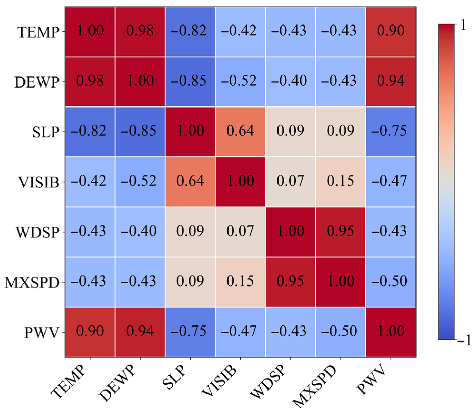
To analyze the relationship between PWV and meteorological variables, Spearman’s rank correlation coefficient was used. Spearman’s correlation was adopted because it can characterize monotonic relationships and is less sensitive to potential outliers than Pearson correlation. The resulting correlation matrix was used to generate the correlation heatmap.

2.4. Technical Route

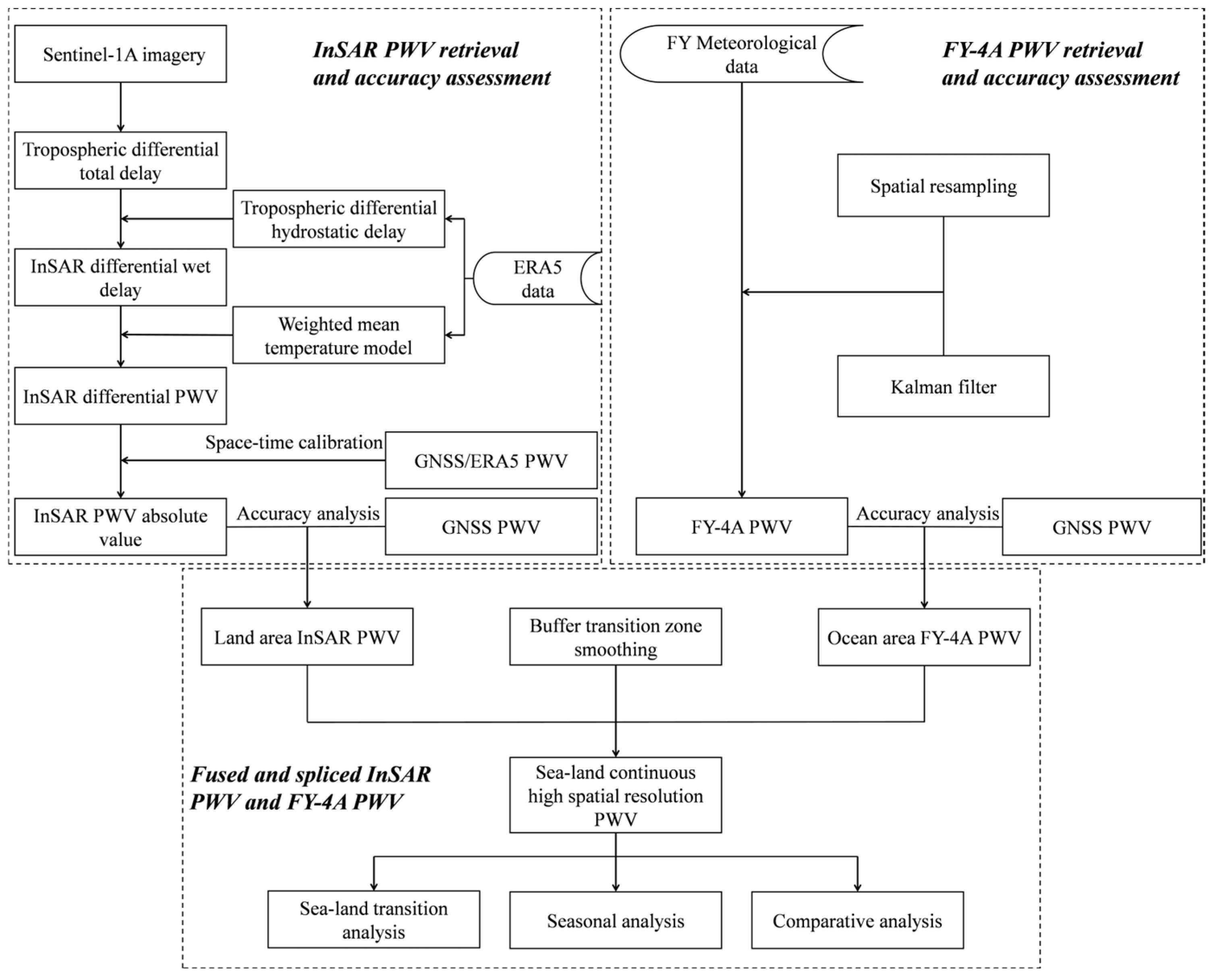
In order to construct a high-resolution PWV with sea–land continuity and to address the limitation that InSAR PWV cannot capture water vapor over the ocean, this study uses FY-4A PWV to compensate for this limitation. It is combined with InSAR PWV to reconstruct an integrated sea–land PWV for the study area. The specific technical workflow is shown in Figure 2.

The utilization of StaMPS-InSAR technology entails the execution of interferometric processing and time-series analysis of Sentinel-1A images. This process facilitates the retrieval of high-spatial-resolution tropospheric differential total delay. The construction of the tropospheric differential dry delay and weighted mean temperature models is undertaken using ERA5 data, with the objective of converting the differential delay into InSAR differential PWV. The GNSS PWV and ERA5 PWV are then utilized for the spatio-temporal calibration of the differential PWV, thus yielding the final InSAR PWV. The accuracy analysis was conducted by comparing the retrieved InSAR PWV and FY-4A PWV with GNSS PWV observations. In order to facilitate the subsequent fusion process, the FY-4A PWV products are adjusted using spatial resampling and Kalman filtering so that their spatial resolution is consistent with that of the InSAR PWV. This process provides a spatially complete and resolution-matched dataset for the subsequent fusion process, the accuracy of which is then evaluated. On this basis, taking advantage of the full spatial coverage of FY-4A PWV, the InSAR PWV is reprojected onto a unified spatial grid, and a sea–land partition-based collaborative fusion strategy is developed: high-resolution InSAR PWV is preferentially used over land, while FY-4A PWV is adopted over the ocean. The introduction of a transition zone at the sea–land boundary is a deliberate measure designed to facilitate seamless integration. The ultimate objective is to obtain a continuous and consistent sea–land integrated PWV, thereby achieving high-resolution collaborative reconstruction of a spatially continuous PWV.

3. Results

3.1. InSAR PWV Retrieval

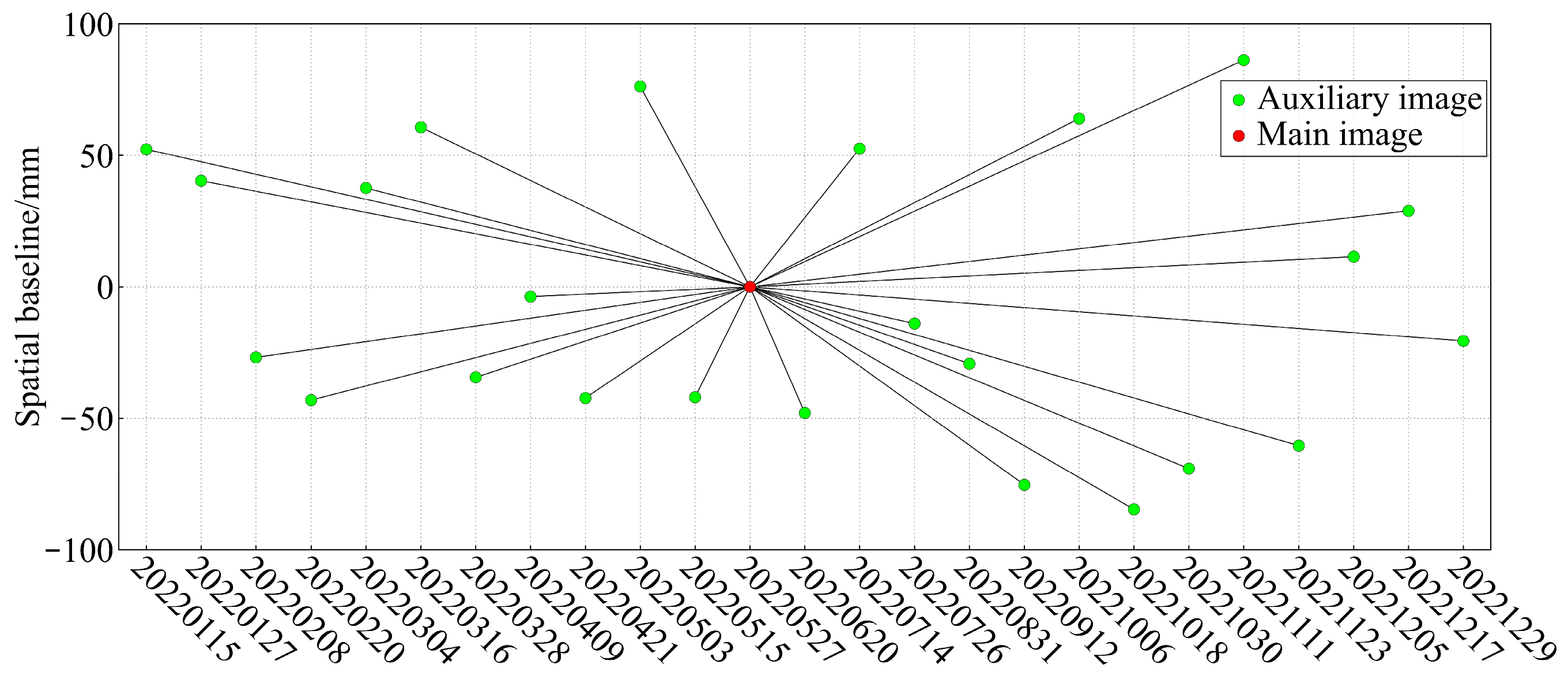
In this study, the StaMPS-InSAR approach was utilized to estimate the total tropospheric delay phase over land areas from Sentinel-1A images acquired in 2022. The tropospheric hydrostatic delay phase was subsequently calculated using ERA5 pressure data. The tropospheric wet delay phase over land areas was obtained by subtracting the hydrostatic delay phase from the total delay phase. In order to reduce the effects of temporal baseline length, spatial decorrelation, and surface deformation errors, the image acquired on 27 May 2022 was selected as the master image, and interferometric pairs with spatial baselines greater than 90 m were removed. As demonstrated in Figure 3, the spatio-temporal baseline relationship between the primary image and the 24 secondary images is illustrated.

The StaMPS-InSAR processing produced tropospheric differential total delay containing both dry and wet atmospheric components. By estimating the dry delay phase from the ERA5 surface pressure and removing it from the zenith tropospheric differential total delay, the differential wet delay was obtained. This wet component was then converted into differential precipitable water vapor (ΔPWV) using the water vapor conversion coefficient derived from the ERA5-based weighted mean temperature after bilinear interpolation to the Sentinel-1A spatial resolution. The resulting ΔPWV describes the relative spatial variability of atmospheric water vapor with respect to a stable reference point, as well as the temporal difference relative to the master image acquisition time.

Despite the spatial calibration, the InSAR-derived PWV still represented relative water vapor change between the primary and secondary acquisition epochs, referred to as InSAR ΔPWVc. To obtain the absolute InSAR PWV at the secondary acquisition time, temporal calibration was performed by approximating the Sentinel-1A acquisition time of 09:57 UTC to 10:00 UTC. A continuous PWV at the master acquisition time was constructed from GNSS PWV observations and ERA5 PWV data using Kriging interpolation and then constrained to the InSAR coverage. Combining this GNSS/ERA5-constrained PWV with InSAR ΔPWVc yielded the absolute InSAR PWV at the secondary acquisition time.

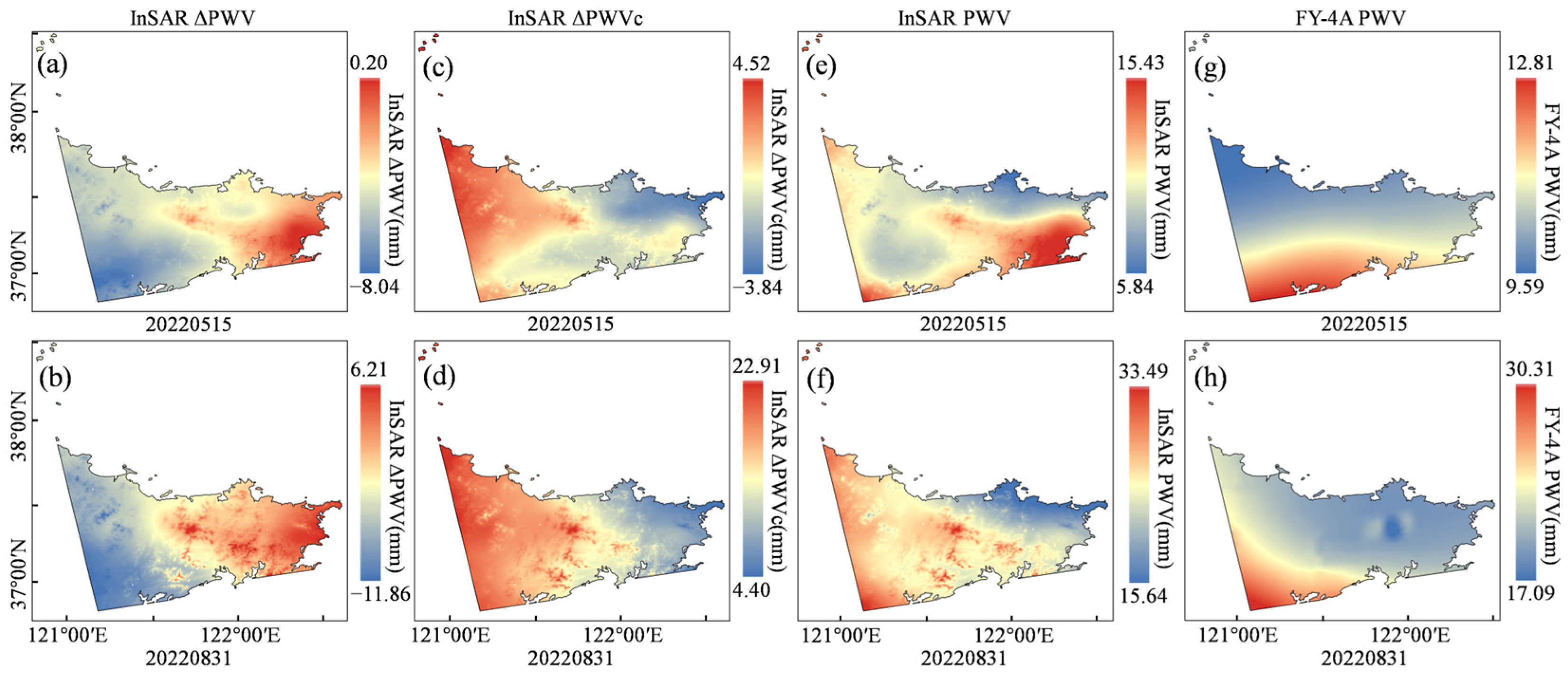
Figure 4 presents a comparison of the original InSAR ΔPWV, spatially calibrated InSAR ΔPWVc, final calibrated InSAR PWV, and FY-4A PWV over land on 15 May and 31 August 2022. The findings demonstrate that the initial InSAR ΔPWV effectively captures distinct regional variations and local inhomogeneities in atmospheric water vapor, thereby substantiating the hypothesis that the StaMPS-InSAR technique exhibits a high degree of sensitivity to spatial variations in tropospheric moisture. Following spatial calibration, the InSAR ΔPWVc demonstrates a more physically consistent spatial pattern, with the large-scale moisture distribution becoming more reasonable while the fine-scale spatial details are still well preserved. The final calibrated InSAR PWV further converts the relative differential information into an absolute PWV, while maintaining the detailed texture and localized variability inherited from the InSAR observations. In contradistinction, the FY-4A PWV over the aforementioned land area displays a considerably more uniform spatial pattern and exhibits diminished sensitivity to local moisture variations. Although the FY-4A PWV is capable of reflecting the general regional distribution of water vapor, its capacity to resolve small-scale spatial features is less developed. These comparisons demonstrate that the InSAR-derived PWV not only preserves the regional-scale distribution characteristics of atmospheric water vapor, but also provides more detailed local information, thus highlighting its clear advantage for high-spatial-resolution PWV retrieval over land.

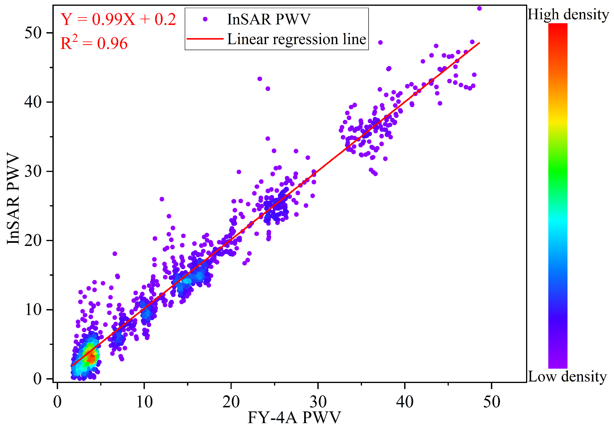
As demonstrated in Figure 5, the scatter plot illustrates the correlation between InSAR PWV and FY-4A PWV. The scatter density plot was constructed using valid paired pixels from all selected 2022 InSAR PWV maps and their corresponding FY-4A PWV products. A robust linear correlation is evident between the two datasets, as evidenced by a fitted equation of Y = 0.99X + 0.2 and an R² of 0.96, signifying a high degree of consistency. The fitted slope approaches 1, and the intercept approaches 0, suggesting that FY-4A PWV and InSAR PWV demonstrate a strong degree of agreement over a broad range of water vapor conditions. The majority of samples are concentrated along the fitted line, particularly within the low and medium PWV ranges, while the dispersion increases marginally at higher PWV values, with a few scattered outliers. The results demonstrate a strong correlation between FY-4A PWV and InSAR PWV in terms of their ability to describe the spatial variability of atmospheric water vapor. This finding provides a reliable foundation for subsequent multi-source fusion and consistency analysis.

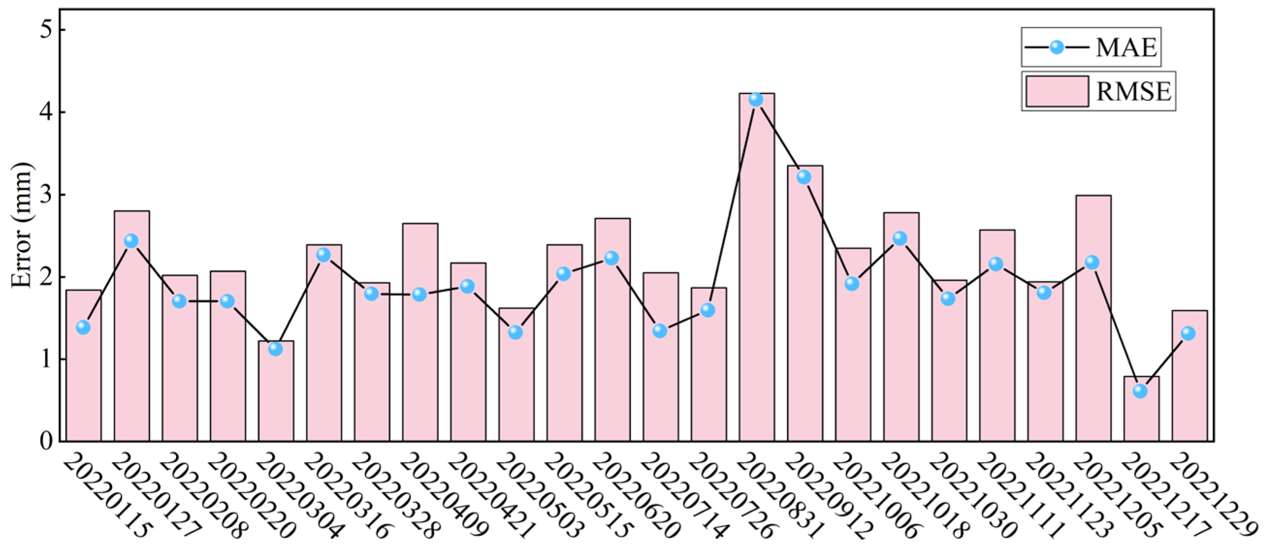
As demonstrated in Figure 6, the temporal variations in the MAE and RMSE of InSAR PWV relative to GNSS PWV in 2022 are illustrated. The MAE ranges from 0.61 mm to 4.14 mm, and the RMSE ranges from 0.79 mm to 4.23 mm. The majority of dates demonstrate minimal discrepancies, with MAE typically falling below 2.50 mm and RMSE generally less than 3.00 mm. This suggests that there is substantial agreement between InSAR PWV and GNSS PWV for the majority of epochs. The optimal performance is observed on 17 December (MAE = 0.61 mm, RMSE = 0.79 mm), whereas the most substantial errors occur on 31 August (MAE = 4.14 mm, RMSE = 4.23 mm) and 12 September (MAE = 3.20 mm, RMSE = 3.35 mm). The comparison demonstrates that the InSAR-derived PWV has generally good temporal stability and reliability with respect to GNSS PWV.

To further describe the distribution of the error statistics, the mean, variance, and skewness coefficient of the MAE and RMSE series were also calculated. The mean values reflect the overall error level, the variances describe the temporal fluctuation of the errors, and the skewness coefficients indicate whether the error distribution is affected by a small number of high-error epochs. The corresponding statistical results are summarized in

Table 2. Descriptive statistics of InSAR PWV errors relative to GNSS PWV.

Metrics	Mean (mm)	Variance (mm2)	Skewness Coefficient
MAE	1.97	0.51	1.17
RMSE	2.24	0.65	1.11

.

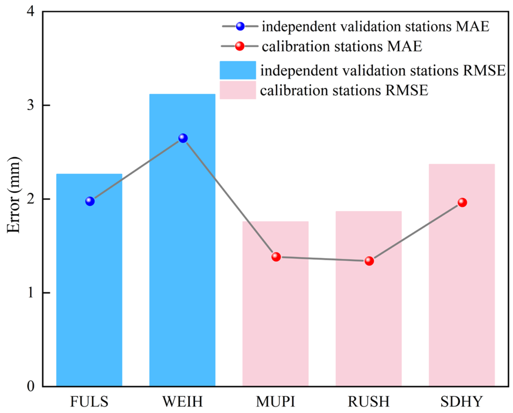
To further provide an unbiased assessment of the InSAR PWV retrieval accuracy, the error statistics were calculated separately for each CORS station. Among the five CORS, FULS and WEIH were excluded from the calibration process and used only as independent validation stations, while MUPI, RUSH, and SDHY were used as calibration stations. As demonstrated in Figure 7, the independent validation stations show slightly larger errors than some calibration stations, which is reasonable because they were not involved in the calibration process. Nevertheless, their MAE and RMSE values remain within an acceptable range, indicating that the calibrated InSAR PWV has good independent validation performance. Compared with the overall statistics, the station-wise error analysis avoids the potential optimistic bias caused by mixing calibration and validation stations.

3.2. FY-4A PWV Retrieval

FY-4A PWV has relatively high spatial resolution and provides coverage over both land and ocean, which compensates for the limitation that InSAR cannot retrieve PWV over ocean regions. However, due to the influence of factors such as cloud contamination, variations in observation geometry, and the stability of the retrieval algorithm, missing pixels may occur in some areas of the FY-4A PWV data. The presence of these missing values disrupts the spatial continuity of the water vapor.

For subsequent fusion, the FY-4A PWV data were further adjusted through spatial resampling and Kalman filtering to achieve a resolution consistent with that of the other datasets and to obtain a more spatially complete PWV. It should be noted that this processing was introduced primarily to facilitate the subsequent fusion procedure and ensure resolution consistency among multi-source data. The Kalman filtering did not alter the overall variation characteristics of PWV over the ocean, but mainly served to improve data completeness and support the construction of a unified sea–land continuous PWV.

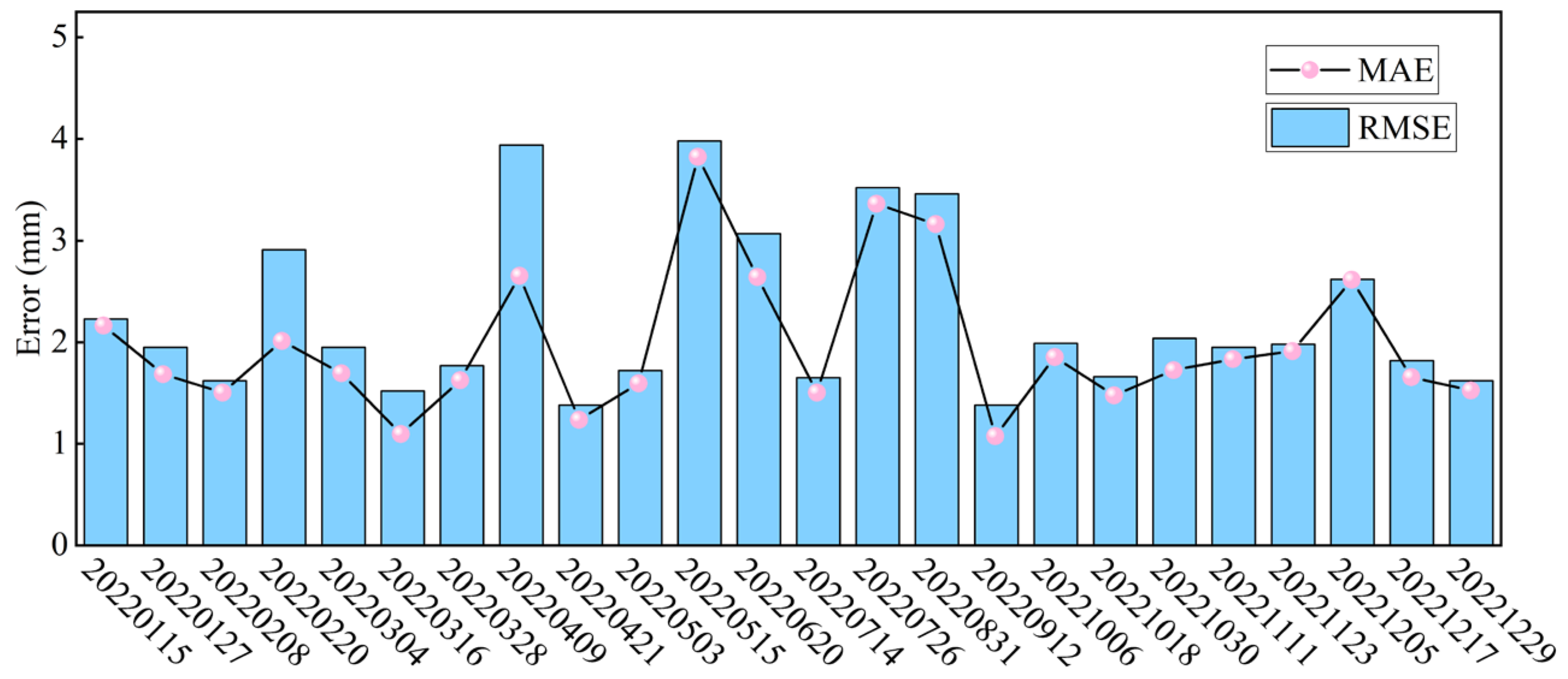
As demonstrated in Figure 8, the temporal variations in the MAE and RMSE of FY-4A PWV relative to GNSS PWV in 2022 are illustrated. The MAE ranges from 1.09 mm to 3.82 mm, and the RMSE ranges from 1.38 mm to 3.98 mm. Most dates show moderate errors, with MAE below 2.00 mm for 16 epochs and RMSE below 3.00 mm for 19 epochs. The lowest errors occur on 21 April and 12 September, whereas the highest errors are observed on 15 May, followed by 26 July and 31 August. These results indicate that the FY-4A PWV has generally stable agreement with GNSS PWV, although larger uncertainties still appear at several individual epochs.

To further characterize the distribution of the FY-4A PWV errors, the mean, variance, and skewness coefficient of the MAE and RMSE series were calculated, as shown in

Table 3. Descriptive statistics of FY-4A PWV errors relative to GNSS PWV.

Metrics	Mean (mm)	Variance (mm2)	Skewness Coefficient
MAE	1.92	0.50	1.33
RMSE	2.26	0.50	0.62

. The positive skewness coefficients indicate that the error distributions are right-skewed, suggesting that several high-error epochs contribute to the upper tail of the error distribution.

3.3. Construction of the PWV over Jiaodong Peninsula and Adjacent Seas Areas Using Multi-Source Data

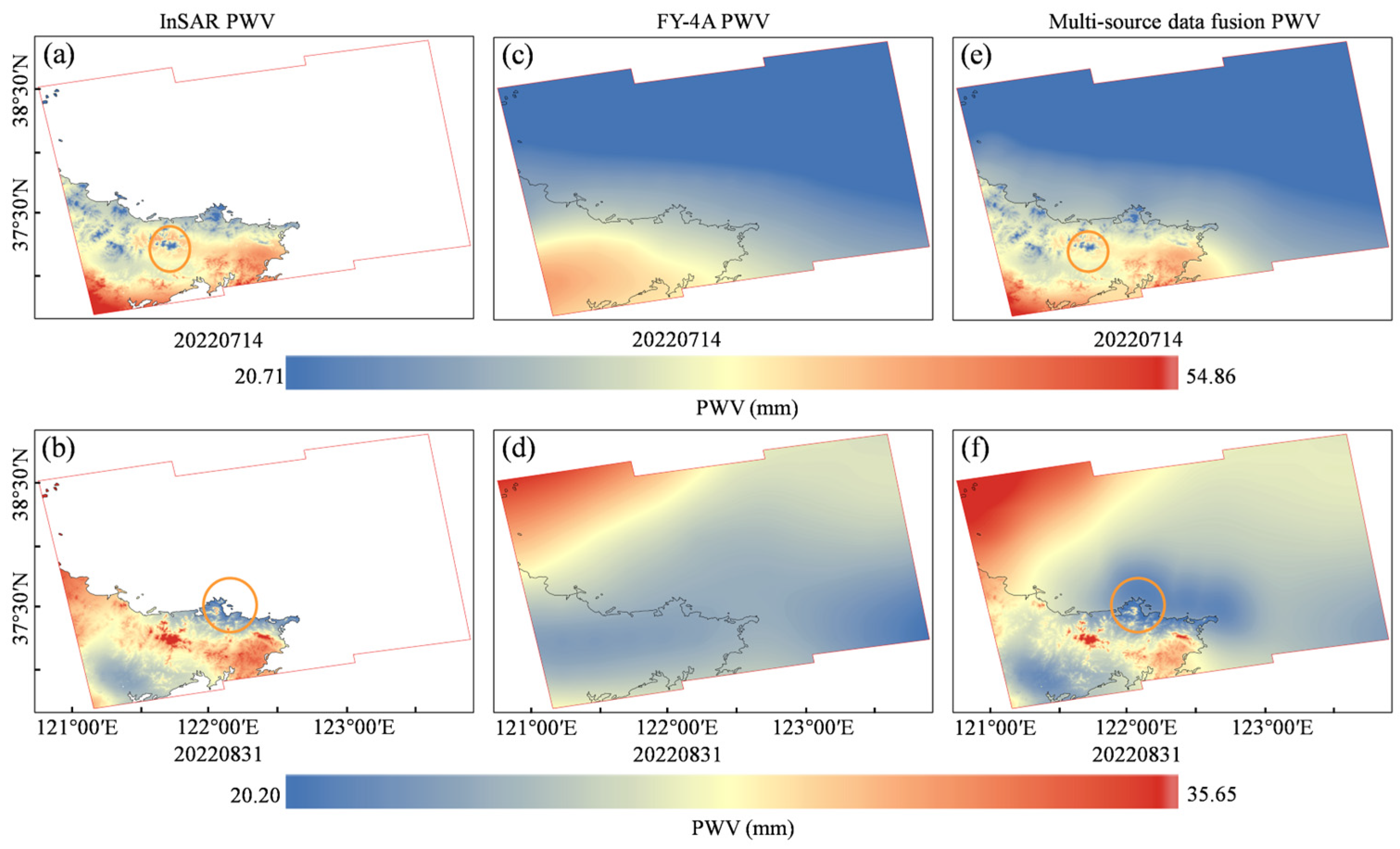
As shown in Figure 9, the multi-source PWV was constructed by combining InSAR PWV and the spatially adjusted FY-4A PWV through the distance-based coastal transition strategy. The FY-4A PWV used in the fusion had been resampled and processed by Kalman filtering before fusion to ensure spatial consistency with the InSAR PWV grid. The InSAR PWV in the first column demonstrates significant fine-scale spatial variability over land, yet no PWV information is available for the ocean. Conversely, the FY-4A PWV in the second column provides comprehensive coverage across the entire study area, though its spatial pattern is comparatively uniform and exhibits a paucity of detailed local variability over land. The fused multi-source PWV in the third column effectively combines the strengths of both datasets. The proposed method preserves the fine spatial structures and localized PWV variations from land-based InSAR data while maintaining the broad, continuous PWV distribution from oceanic FY-4A data. Furthermore, no discernible artificial seam is evident in the proximity of the coastline, and the PWV gradients across the sea–land boundary maintain a consistent and cohesive nature, suggesting that the proposed fusion strategy can attain a satisfactory transition between terrestrial and maritime domains. The findings indicate that the integration of distance weighting and Kalman filtering is a successful methodology for the construction of a continuous PWV, encompassing both terrestrial and marine regions with high spatial resolution.

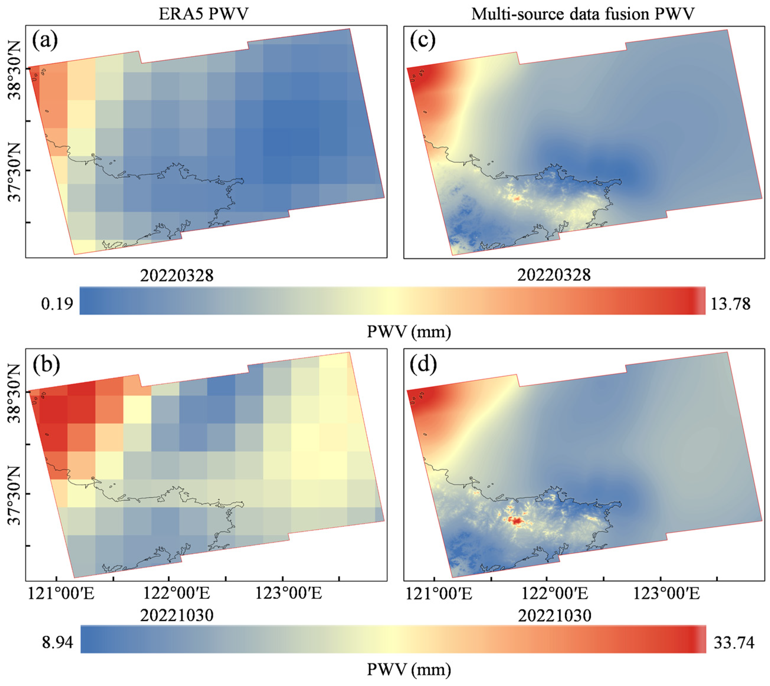
Figure 10 compares the spatial distribution of ERA5 PWV and multi-source fused PWV. Overall, the PWV over the coastal regions of the Jiaodong Peninsula and its adjacent seas in 2022 exhibits pronounced spatial heterogeneity, with an annual variation range of 0.35–59.74 mm. In general, PWV tends to increase from inland areas toward the coast, and the annual mean PWV is generally higher over the ocean than over land, reflecting the ocean’s role as a major moisture source. By contrast, inland regions, especially those at higher elevations or farther from the coastline, usually present relatively low PWV values. Nevertheless, some isolated land areas show locally enhanced PWV compared with their surroundings, which is likely associated with topographic influences on water vapor transport and accumulation.

Against this regional background, the multi-source fused PWV provides a more complete description of the spatial distribution of atmospheric water vapor across the study area. It preserves the large-scale continuous pattern represented by ERA5/FY-4A PWV, while further enhancing the fine-scale spatial variability within the InSAR-covered region. As shown in Figure 10, the fused PWV field forms a spatially continuous sea–land water vapor distribution and simultaneously captures more detailed local gradient changes over land. A relatively stable gradient is observed from ocean to land, with PWV over the ocean generally remaining higher and more homogeneous, whereas PWV over land shows stronger spatial variability and more pronounced local differences. This pattern can be attributed to the persistent moisture supply from sea surface evaporation and the large heat capacity of the ocean, in contrast to the stronger influence of topography and land-surface heterogeneity on the terrestrial water vapor.

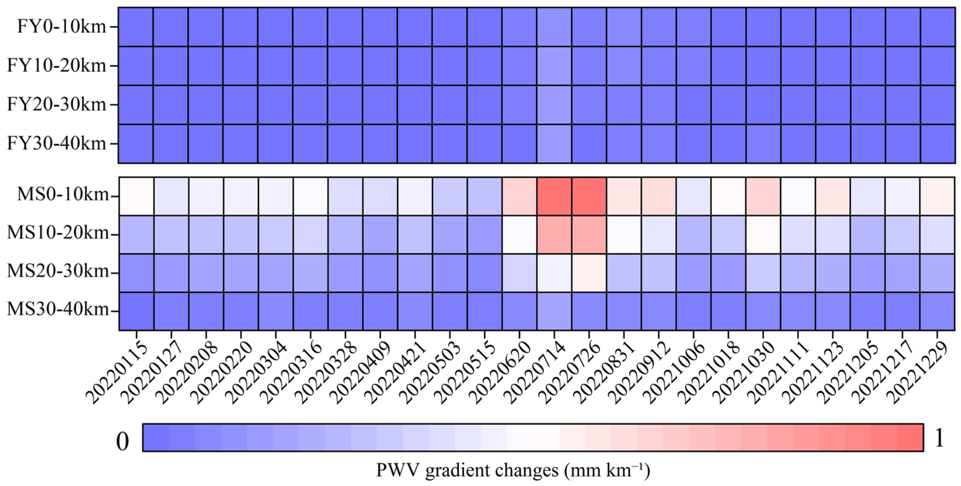
To quantify coastal PWV gradients, the coastal zone within 40 km of the coastline was divided into four distance bands: 0–10 km, 10–20 km, 20–30 km, and 30–40 km. After reprojecting the PWV maps to a projected coordinate system, the pixel-level spatial gradient magnitude was calculated from the PWV differences in the x and y directions, with a unit of mm km⁻¹. The mean gradient for each distance band was then obtained by averaging the gradient magnitudes of all valid pixels within that band. The same coastline mask, distance bands, and valid-pixel criteria were applied to FY-4A PWV and multi-source fused PWV. As demonstrated in Figure 11, the PWV gradient variations within different coastal distance bands manifest as distinct disparities between FY-4A PWV and the multi-source fused PWV. The FY-4A PWV gradients demonstrate a consistent low level across all distance bands and dates, indicating relatively smooth spatial changes in coastal water vapor. In contrast, the multi-source fused PWV demonstrates markedly stronger gradient signals, particularly within the 0–10 km and 10–20 km coastal zones, suggesting that the fused PWV exhibits heightened sensitivity to the abrupt moisture transition across the sea–land interface. A clear distance-decay pattern can be observed in the multi-source fused PWV. The most pronounced gradients are observed in the near-coastal zone, gradually diminishing with increasing distance from the coastline, from 0 to 10 km to 30–40 km. This feature indicates that the fusion strategy effectively preserves the pronounced sea–land contrast in atmospheric water vapor while also capturing its gradual inland attenuation. In comparison, the FY-4A PWV demonstrates significantly diminished gradient variability and a more uniform spatial pattern, indicative of its constrained capacity to discern fine-scale variations in coastal topography. The temporal variation in gradient intensity is also evident. It has been demonstrated that larger gradients primarily occur during the warm season, with the greatest levels of multi-source fused PWV being recorded in July. The most significant enhancements were observed on 14 July and 26 July 2022. Relatively strong gradients are also observed on 20 June, 31 August, and 12 September. In contrast, the gradients observed during the winter months are generally much weaker. The findings indicate that the disparity between the sea and land PWV is considerably accentuated during the summer months, while it becomes less pronounced in the winter season. The comparison demonstrates that the multi-source fused PWV is more capable than the FY-4A PWV of characterizing the coastal gradient structure and representing the spatial heterogeneity of atmospheric water vapor in the sea–land transition zone.

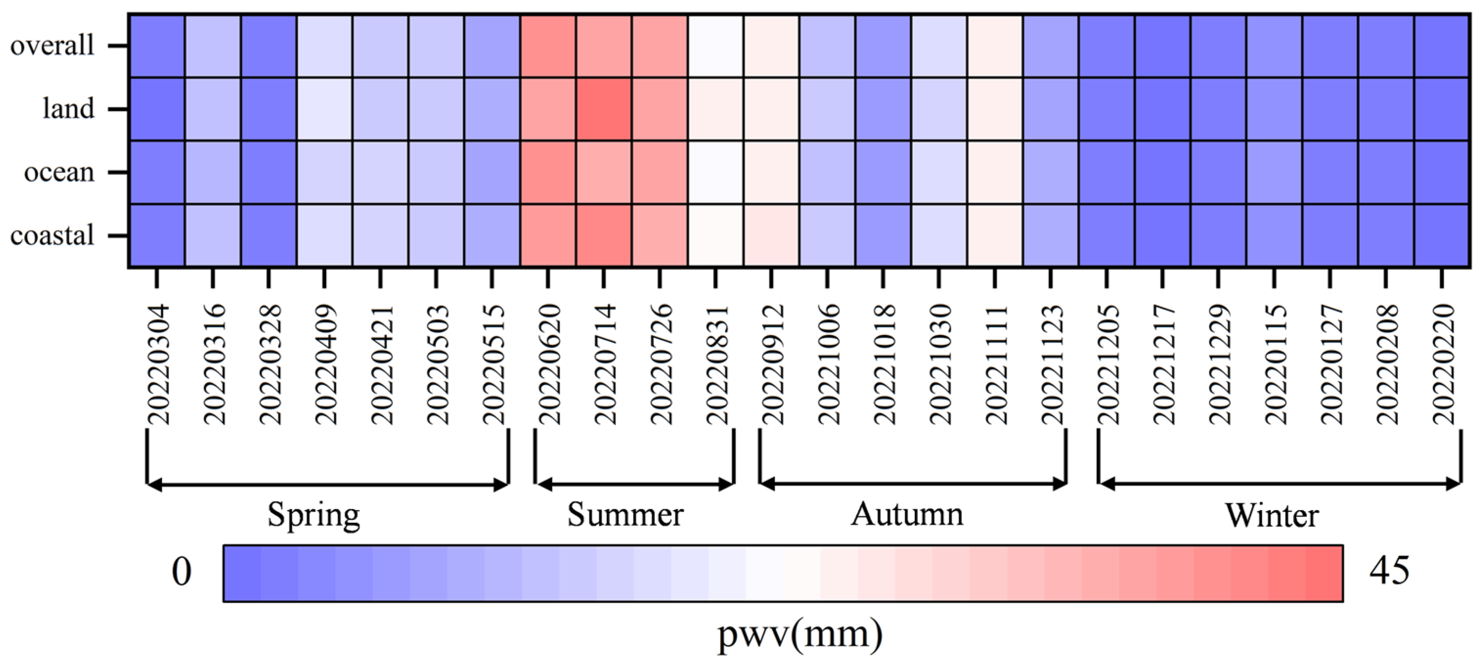
As demonstrated in Figure 12, PWV over the study area displays a marked seasonal cycle in the overall mean, land mean, ocean mean, and coastal 40 km mean values. All four indicators demonstrate a general increase from winter to summer and subsequent decrease in autumn, thus exhibiting robust seasonal modulation of atmospheric moisture over the Jiaodong Peninsula and adjacent seas. The winter period is distinguished by consistently low PWV and minimal spatial variations among land, ocean, and coastal regions. Conversely, summer exhibits the highest PWV levels and the most pronounced regional heterogeneity. The regional mean PWV remains at a low level during the winter months, increases noticeably in the spring, reaches its maximum in the summer, and then declines in the autumn. A parallel temporal evolution is observed for the land, ocean, and coastal-zone mean PWV. Among the four seasons, summer records the highest precipitation. This is particularly evident on 20 June, 14 July and 26 July 2022, which demonstrate substantial moisture accumulation during the warm season. Conversely, PWV values on winter dates are consistently low, indicative of dry atmospheric conditions. Evident differences can be observed among land, ocean, and coastal areas. During the winter months, the ocean mean PWV is marginally higher than the land mean PWV. Conversely, in the spring, the land and ocean values become relatively similar. During summer months, the land and coastal zones typically exhibit higher PWV values in comparison to the ocean, indicating heightened moisture convergence and augmented sea–land interaction during this season. During the autumn months, the PWV over both land and ocean become more comparable once more, while the coastal 40 km zone continues to exhibit relatively high values. The results indicate that PWV over the Jiaodong Peninsula and adjacent seas is characterized by significant seasonal variability and clear spatial differences, with the warm season showing both the highest moisture content and the strongest sea–land heterogeneity.

As illustrated in Figure 13, the Spearman correlation coefficients between PWV and the selected meteorological variables are demonstrated. PWV demonstrates the strongest positive correlation with mean dew point (DEWP), with a correlation coefficient of 0.94. This finding indicates that higher dew point conditions are closely associated with increased atmospheric water vapor content. PWV also demonstrates a significant positive correlation with mean temperature (TEMP), with a coefficient of 0.90, indicating that elevated atmospheric conditions tend to coincide with increased moisture content. In contrast, a strong negative correlation has been observed between PWV and mean sea level pressure (SLP), with a coefficient of −0.75. This suggests that lower-pressure conditions are more conducive to water vapor accumulation, whereas higher-pressure conditions are generally associated with drier atmospheric states. PWV demonstrates a moderate negative correlation with mean visibility (VISIB), with a coefficient of −0.47. This finding suggests that increased atmospheric moisture is frequently accompanied by reduced visibility.

The correlations of PWV with mean wind speed (WDSP) and maximum sustained wind speed (MXSPD) are −0.43 and −0.50, respectively, which are weaker than those with the thermodynamic variables. This finding suggests that wind-related factors may have a comparatively limited influence on PWV variability in the study area. In general, PWV is predominantly governed by thermodynamic and moisture-related factors. This assertion is substantiated by the robust positive correlations observed between PWV and both DEWP and TEMP, as well as the pronounced negative correlation with SLP. The impact of factors such as visibility and wind speed appears to be comparatively negligible.

4. Discussion

4.1. Physical Interpretation and Robustness of the Fused PWV

To evaluate the uncertainty introduced by the transition-zone processing, a simple sensitivity test was performed by changing the near-coastal influence distance in the distance-dependent weighting function. The fused PWV obtained using the standard influence distance was used as the baseline, and two additional tests were conducted by decreasing and increasing this parameter while keeping the other processing parameters unchanged. Compared with the baseline result, the mean absolute differences were 0.24 mm and 0.31 mm, and the RMSE differences were 0.34 mm and 0.43 mm, respectively. These results indicate that the distance-dependent weighting parameter has only a limited influence on the fused PWV field, suggesting that the detected coastal PWV gradients are not dominated by subjective parameter selection.

The spatial and seasonal variations in PWV over the Jiaodong Peninsula and adjacent seas are closely related to regional moisture supply, land–sea thermal contrast, and topographic modulation. The seasonal cycle, with low PWV in winter and high PWV in summer, reflects stronger evaporation and enhanced water vapor transport from adjacent marine areas during the warm season. The stronger gradients in the 0–10 km and 10–20 km coastal bands indicate that the most rapid moisture transition occurs near the land–sea boundary. This pattern is physically consistent with the contrast between the ocean, which acts as a continuous moisture source, and the land surface, where topography, surface heating, and terrain-induced circulation can modify water vapor transport and accumulation.

Compared with previous GNSS- and ERA5-based PWV studies [10,11,12,13,14], which mainly provide station-scale or coarse-resolution regional moisture information, the proposed framework improves the spatial representation of water vapor structures in the coastal zone by introducing high-resolution InSAR PWV over land. Compared with FY-4A PWV alone [18,19,20,21,22], the fused PWV retains the broad sea–land coverage of FY-4A while enhancing fine-scale spatial variability over land and near the coastline. Therefore, the main improvement of this study lies not only in increasing spatial continuity, but also in preserving the coastal gradient and local structural information that are difficult to capture using a single data source.

4.2. Limitations and Future Improvements

Despite these improvements, the current framework still has limitations. Cokriging may be useful for incorporating ERA5 PWV or topographic variables as secondary covariates, and its potential application will be further evaluated in future work. The coastal transition is mainly controlled by distance-based weighting and spatial smoothing, which are effective in reducing abrupt discontinuities but remain partly empirical. Future studies could introduce deep learning or other data-driven methods to learn nonlinear relationships among InSAR PWV, FY-4A PWV, ERA5 meteorological fields, and auxiliary spatial covariates, such as DEM, terrain slope, distance to coastline, and land–sea mask. Such covariate-aware models may help refine the fusion weights or correction terms in complex coastal environments and further improve the physical consistency of the fused PWV field.

The independent validation of the marine component of the fused PWV remains limited because of the lack of in situ PWV observations over adjacent sea areas. In this study, the marine PWV component is mainly constrained by FY-4A PWV, while Kalman filtering is used only to improve the spatial consistency of FY-4A PWV before fusion. Therefore, the marine component should be interpreted as a reconstructed PWV field constrained by satellite observations rather than a fully independently validated marine PWV product. In addition, the horizontal isotropy assumption around GNSS stations and the neglect of liquid water delay may introduce additional uncertainty under strong coastal gradients or severe weather conditions. Finally, because this study is based on data from 2022, the observed seasonal patterns should be regarded as an annual case study rather than evidence of long-term climatic trends. Future work should incorporate radiosonde, island GNSS, shipborne GNSS, microwave radiometer, buoy-based observations, and multi-year datasets to further validate and extend the framework.

5. Conclusions

While previous studies have explored multi-source PWV retrieval, this study uniquely combines GNSS, InSAR, ERA5, and FY-4A data to achieve continuous sea–land coverage with high spatial resolution. Through the complementary use of these multi-source datasets, a high-resolution PWV with continuous land–sea coverage was achieved. The primary conclusions that can be drawn from this study are as follows:

(1)

InSAR PWV can effectively capture the fine-scale spatial variations of the water vapor, particularly in areas with complex terrain and locally active convection, demonstrating strong structural resolving capability. Validation against GNSS PWV shows that the InSAR PWV achieves an R² of 0.955, an MAE of 1.86 mm, and an RMSE of 2.32 mm. Its temporal MAE ranges from 0.61 mm to 4.14 mm, and the RMSE ranges from 0.79 mm to 4.23 mm, indicating generally good stability and reliability over different epochs. FY-4A PWV shows good agreement with GNSS PWV, with an R² of 0.961, an MAE of 1.90 mm, and an RMSE of 2.28 mm. Its temporal MAE and RMSE range from 1.09 mm to 3.82 mm and from 1.38 mm to 3.98 mm, respectively.

(2)

The multi-source fused PWV maintain good spatial continuity in the sea–land transition zone and clearly capture the cross-shore water vapor gradients and their spatial variation trends. The maximum coastal PWV gradients in the 0–10 km zone reach 0.823 mm/km and 0.798 mm/km on 14 July and 26 July 2022, respectively, indicating that the fused PWV can effectively characterize the sharp moisture transition across the sea–land interface. PWV shows an annual variation range of 0.35–59.74 mm, with an overall increase from inland toward the ocean. A clear seasonal cycle is also observed, with regional mean PWV values of 4.16 mm in winter, 11.16 mm in spring, 33.24 mm in summer, and 16.50 mm in autumn, indicating that the warm season exhibits the highest moisture content and the strongest regional heterogeneity.

(3)

The multi-source fused PWV outperforms single-source products in terms of spatial completeness, structural representation, and practical applicability. The fused result preserves the high-resolution mapping capability of InSAR over land while extending water vapor information to offshore areas through the incorporation of FY-4A products, thereby alleviate the spatial discontinuity of InSAR PWV being restricted to land areas. At the same time, GNSS PWV provides an accuracy constraint that improves the quantitative reliability of the fused water vapor and helps reconcile systematic differences among the various data sources.

This study provides a promising sea–land partitioned reconstruction strategy for constructing spatially continuous PWV in coastal regions by combining GNSS/ERA5-constrained InSAR PWV with FY-4A PWV. The proposed framework improves the continuity of PWV across the land–sea transition zone and provides useful support for analyzing coastal water vapor transport and precipitation-related atmospheric processes. However, further validation over marine areas, more comprehensive uncertainty assessment, and applications in other coastal regions are still needed before broader operational use can be considered.

References

1. Chen, B.; Liu, Z. Global water vapor variability and trend from the latest 36 year (1979 to 2014) data of ECMWF and NCEP reanalyses, radiosonde, GPS, and microwave satellite. J. Geophys. Res. Atmos. 2016, 121, 11442–11462. [Google Scholar] [CrossRef]
2. Zhao, Q.; Yao, Y.; Yao, W. GPS-based PWV for precipitation forecasting and its application to a typhoon event. J. Atmos. Sol.-Terr. Phys. 2018, 167, 124–133. [Google Scholar] [CrossRef]
3. Li, X.; Dick, G.; Lu, C.; Ge, M.; Nilsson, T.; Ning, T.; Wickert, J.; Schuh, H. Multi-GNSS meteorology: Real-time retrieving of atmospheric water vapor from BeiDou, Galileo, GLONASS, and GPS observations. IEEE Trans. Geosci. Remote Sens. 2015, 53, 6385–6393. [Google Scholar] [CrossRef]
4. Bevis, M.; Businger, S.; Herring, T.A.; Rocken, C. GPS meteorology: Remote sensing of atmospheric water vapor using the Global Positioning System. J. Geophys. Res. Atmos. 1992, 97, 15787–15801. [Google Scholar] [CrossRef]
5. Yao, Y.; Zhu, S.; Yue, S. A globally applicable, season-specific model for estimating the weighted mean temperature of the atmosphere. J. Geod. 2012, 86, 1125–1135. [Google Scholar] [CrossRef]
6. Hersbach, H.; Bell, B.; Berrisford, P.; Hirahara, S.; Horányi, A.; Muñoz-Sabater, J.; Nicolas, J.; Peubey, C.; Radu, R.; Schepers, D.; et al. The ERA5 global reanalysis. Q. J. R. Meteorol. Soc. 2020, 146, 1999–2049. [Google Scholar] [CrossRef]
7. Mateus, P.; Tomé, R.; Nico, G.; Catalão, J. Three-dimensional variational assimilation of InSAR PWV using the WRFDA model. IEEE Trans. Geosci. Remote Sens. 2016, 54, 7323–7330. [Google Scholar] [CrossRef]
8. Zhang, Y.; Li, Z.L.; Li, J. A preliminary layer perceptible water vapor retrieval algorithm for Fengyun-4 Advanced Geosynchronous Radiation Imager. In Proceedings of the 2019 IEEE International Geoscience and Remote Sensing Symposium (IGARSS 2019), Yokohama, Japan, 28 July–2 August 2019; pp. 7564–7566. [Google Scholar]
9. Tarayre, H.; Massonnet, D. Atmospheric propagation heterogeneities revealed by ERS-1 interferometry. Geophys. Res. Lett. 1996, 23, 989–992. [Google Scholar] [CrossRef]
10. Hanssen, R.F.; Weckwerth, T.M.; Zebker, H.A.; Klees, R. High-resolution water vapor mapping from interferometric radar measurements. Science 1999, 283, 1297–1299. [Google Scholar] [CrossRef]
11. Li, Z.; Fielding, E.J.; Cross, P. Integration of InSAR time-series analysis and water-vapor correction for mapping postseismic motion after the 2003 Bam(Iran), earthquake. IEEE Trans. Geosci. Remote Sens. 2009, 47, 3220–3230. [Google Scholar]
12. Yun, Y.; Zeng, Q.; Green, B.W.; Zhang, F. Mitigating atmospheric effects in InSAR measurements through high-resolution data assimilation and numerical simulations with a weather prediction model. Int. J. Remote Sens. 2015, 36, 2129–2147. [Google Scholar] [CrossRef]
13. Tang, W.; Liao, M.; Zhang, L.; Li, W.; Yu, W. High-spatial-resolution mapping of precipitable water vapour using SAR interferograms, GPS observations and ERA-Interim reanalysis. Atmos. Meas. Tech. 2016, 9, 4487–4501. [Google Scholar] [CrossRef]
14. Mateus, P.; Catalão, J.; Nico, G.; Benevides, P. Mapping precipitable water vapor time series from Sentinel-1 interferometric SAR. IEEE Trans. Geosci. Remote Sens. 2020, 58, 1373–1379. [Google Scholar] [CrossRef]
15. Alshawaf, F. A new method for reconstructing absolute water vapor maps from persistent scatterer InSAR. IEEE Trans. Geosci. Remote Sens. 2020, 58, 4951–4957. [Google Scholar] [CrossRef]
16. Guo, Q.; Yu, M.; Li, D.; Huang, S.; Xue, X.; Sun, Y.; Zhou, C. An optimized framework for precipitable water vapor mapping using TS-InSAR and GNSS. Atmosphere 2023, 14, 1674. [Google Scholar] [CrossRef]
17. Mateus, P.; Nico, G.; Catalão, J.; Miranda, P.M. Precipitable water vapor from Sentinel-1 improves the forecast of extratropical storm. Q. J. R. Meteorol. Soc. 2024, 150, 1988–2004. [Google Scholar] [CrossRef]
18. Liu, X.; Wang, Y.; Huang, J.; Yu, T.; Jiang, N.; Yang, J.; Zhan, W. Assessment and calibration of FY-4A AGRI total precipitable water products based on CMONOC. Atmos. Res. 2022, 271, 106096. [Google Scholar] [CrossRef]
19. Wang, Y.; Jiang, N.; Liu, Y.; Liu, X.; Zhan, W. Study on FY-4A water vapor correction model in Beijing-Tianjin-Hebei region. Glob. Position. Syst. 2022, 47, 119–126. [Google Scholar]
20. Wang, X.; Chen, F. Regional weighted mean temperature model for China based on FY-4A GIIRS data and ERA5 reanalysis data. J. Geomat. Surv. 2023, 52, 904–916. [Google Scholar]
21. Chen, X.; Zhang, W.; Lou, Y. Real-time FY-4A hierarchical water vapor correction for ground-based GNSS. J. Navig. Position. 2025, 13, 66–76. [Google Scholar]
22. Yang, F.; Sun, Y.; Liu, M.; Song, S.; Chen, W.; Li, Z.; Wang, L. A new way to obtain the weighted mean temperature (Tm): Using the Geostationary Interferometric Infrared Sounder (GIIRS) equipped on FengYun Satellite. Atmos. Res. 2025, 318, 107997. [Google Scholar] [CrossRef]
23. Wang, S.; Xu, T.; Nie, W.; Jiang, C.; Yang, Y.; Fang, Z.; Li, M.; Zhang, Z. Evaluation of precipitable water vapor from five reanalysis products with ground-based GNSS observations. Remote Sens. 2020, 12, 1817. [Google Scholar] [CrossRef]
24. Wang, Y.; Yang, K.; Pan, Z.; Qin, J.; Chen, D.; Lin, C.; Chen, Y.; Lazhu; Tang, W.; Han, M.; et al. Evaluation of precipitable water vapor from four satellite products and four reanalysis datasets against GPS measurements on the Southern Tibetan Plateau. J. Clim. 2017, 30, 5699–5713. [Google Scholar] [CrossRef]
25. Benevides, P.; Catalão, J.; Miranda, P.M.A. On the inclusion of GPS precipitable water vapour in the nowcasting of rainfall. Nat. Hazards Earth Syst. Sci. 2015, 15, 2605–2616. [Google Scholar] [CrossRef]
26. Saastamoinen, J. Contributions to the theory of atmospheric refraction. Bull. Géodésique (1946–1975) 1972, 105, 279–298. [Google Scholar] [CrossRef]
27. Saastamoinen, J. Introduction to practical computation of astronomical refraction. Bull. Géodésique (1946–1975) 1972, 106, 383–397. [Google Scholar] [CrossRef]
28. Yao, Y.; Shan, L.; Zhao, Q. Establishing a method of short-term rainfall forecasting based on GNSS-derived PWV and its application. Sci. Rep. 2017, 7, 12465. [Google Scholar] [CrossRef]
29. Yuan, Y.; Zhang, K.; Rohm, W.; Choy, S.; Norman, R.; Wang, C.S. Real-time retrieval of precipitable water vapor from GPS precise point positioning. J. Geophys. Res. Atmos. 2014, 119, 10044–10057. [Google Scholar] [CrossRef]
30. Wang, X.; Zhang, K.; Wu, S.; Fan, S.; Cheng, Y. Water vapor-weighted mean temperature and its impact on the determination of precipitable water vapor and its linear trend. J. Geophys. Res. Atmos. 2016, 121, 833–852. [Google Scholar] [CrossRef]
31. Li, L.; Zhang, K.; Wu, S.; Li, H.; Wang, X.; Hu, A.; Li, W.; Fu, E.; Zhang, M.; Shen, Z. An improved method for rainfall forecast based on GNSS-PWV. Remote Sens. 2022, 14, 4280. [Google Scholar] [CrossRef]
32. Li, X.; Long, D. An improvement in accuracy and spatiotemporal continuity of the MODIS precipitable water vapor product based on a data fusion approach. Remote Sens. Environ. 2020, 248, 111966. [Google Scholar] [CrossRef]
33. Bekaert, D.P.S.; Hooper, A.; Wright, T.J. A spatially variable power law tropospheric correction technique for InSAR data. J. Geophys. Res. Solid Earth 2015, 120, 1345–1356. [Google Scholar] [CrossRef]
34. Gui, K.; Che, H.; Chen, Q.; Zeng, Z.; Liu, H.; Wang, Y.; Zheng, Y.; Sun, T.; Liao, T.; Wang, H.; et al. Evaluation of radiosonde, MODIS-NIR-Clear, and AERONET precipitable water vapor using IGS ground-based GPS measurements over China. Atmos. Res. 2017, 197, 461–473. [Google Scholar] [CrossRef]
35. Zhang, W.; Zhang, H.; Liang, H.; Lou, Y.; Cai, Y.; Zhou, Y.; Liu, W. On the suitability of ERA5 in hourly GPS precipitable water vapor retrieval over China. J. Geod. 2019, 93, 1897–1909. [Google Scholar] [CrossRef]
36. Zhao, Q.; Yao, Y.; Yao, W.; Zhang, S. GNSS-derived PWV and comparison with radiosonde and ECMWF ERA-Interim data over mainland China. J. Atmos. Sol.-Terr. Phys. 2019, 182, 85–92. [Google Scholar] [CrossRef]
37. Zhao, Q.; Ma, X.; Yao, W.; Yao, Y. A drought monitoring method based on precipitable water vapor and precipitation. J. Clim. 2020, 33, 10727–10741. [Google Scholar] [CrossRef]
38. Huang, L.; Wang, X.; Xiong, S.; Li, J.; Liu, L.; Mo, Z.; Fu, B.; He, H. High-precision GNSS PWV retrieval using dense GNSS sites and in-situ meteorological observations for the evaluation of MERRA-2 and ERA5 reanalysis products over China. Atmos. Res. 2022, 276, 106247. [Google Scholar] [CrossRef]
39. Huang, L.; Liu, L.; Chen, H.; Jiang, W. An improved atmospheric weighted mean temperature model and its impact on GNSS precipitable water vapor estimates for China. GPS Solut. 2019, 23, 51. [Google Scholar] [CrossRef]
40. Yu, C.; Penna, N.T.; Li, Z. Generation of real-time mode high-resolution water vapor fields from GPS observations. J. Geophys. Res. Atmos. 2017, 122, 2008–2025. [Google Scholar] [CrossRef]
41. Moradkhani, H. Hydrologic remote sensing and land surface data assimilation. Sensors 2008, 8, 2986–3004. [Google Scholar] [CrossRef]
42. Wang, B.; Sun, Z.; Jiang, X.; Liu, R. Kalman filter and its application in data assimilation. Atmosphere 2023, 14, 1319. [Google Scholar] [CrossRef]
43. Sekulić, A.; Kilibarda, M.; Heuvelink, G.B.M.; Nikolić, M.; Bajzt, B. Random forest spatial interpolation. Remote Sens. 2020, 12, 1687. [Google Scholar] [CrossRef]
Figure 1. Geographic information of the study area: (a) location of the Jiaodong Peninsula and adjacent sea areas within China, (b) regional overview of the study area, and (c) distribution of CORS, ERA5 calibration points, and topographic elevation in the study area. FULS and WEIH were used as independent verification stations.
Applsci 16 05391 g001
Figure 2. Technical route.
Applsci 16 05391 g002
Figure 3. Spatio-temporal baseline relation diagram between the primary image and the 24 secondary images.
Applsci 16 05391 g003
Figure 4. Comparison of the original InSAR ΔPWV, spatially calibrated InSAR ΔPWVc, calibrated InSAR PWV, and FY-4A PWV on 15 May 2022 and 31 August 2022. Panels (a,b) show the original InSAR ΔPWV, panels (c,d) show the spatially calibrated InSAR ΔPWVc, panels (e,f) show the calibrated InSAR PWV, and panels (g,h) show the FY-4A PWV.
Applsci 16 05391 g004
Figure 5. Density plot of InSAR PWV fitted against FY-4A PWV, where the color indicates point density.
Applsci 16 05391 g005
Figure 6. Statistical plot of the error of InSAR PWV with respect to GNSS PWV.
Applsci 16 05391 g006
Figure 7. Station-wise MAE and RMSE values of InSAR PWV retrieval at calibration stations and independent validation stations. FULS and WEIH were excluded from the calibration process and used only for independent validation.
Applsci 16 05391 g007
Figure 8. Statistical plot of the error of FY-4A PWV with respect to GNSS PWV.
Applsci 16 05391 g008
Figure 9. Comparison of InSAR PWV, FY-4A PWV, and multi-source fusion PWV on 14 July 2022 and 31 August 2022. Panels (a,b) show the InSAR PWV, panels (c,d) show the FY-4A PWV, and panels (e,f) show the multi-source fusion PWV. The orange circles highlight representative regions where the fusion results preserve the fine-scale spatial details from InSAR PWV while maintaining the large-scale continuous distribution characteristics of FY-4A PWV.
Applsci 16 05391 g009
Figure 10. Comparison of the spatial distribution of ERA5 PWV and multi-source fusion PWV on 28 March 2022 and 30 October 2022. Panels (a,b) show the ERA5 PWV, while panels (c,d) show the corresponding multi-source fusion PWV.
Applsci 16 05391 g010
Figure 11. Comparison of PWV gradient changes (mm km−1) in different coastal distance bands for FY-4A PWV and multi-source fused PWV.
Applsci 16 05391 g011
Figure 12. Seasonal variation in mean PWV over land, ocean, coastal_40km zone, and the entire study area.
Applsci 16 05391 g012
Figure 13. Spearman correlation coefficients between PWV and meteorological variables.
Applsci 16 05391 g013