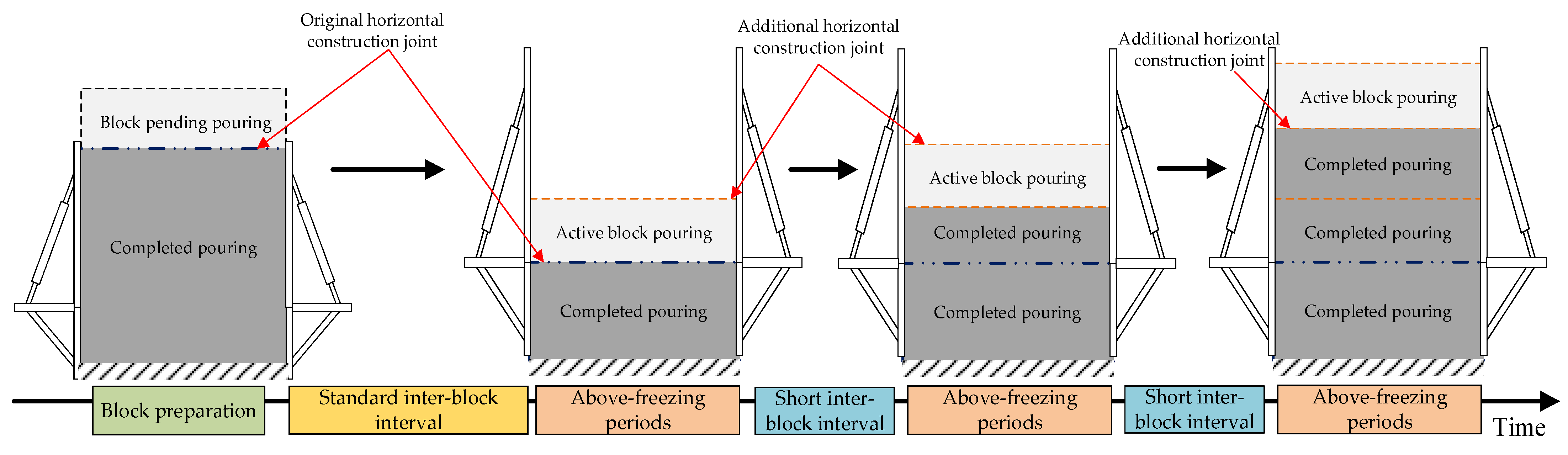
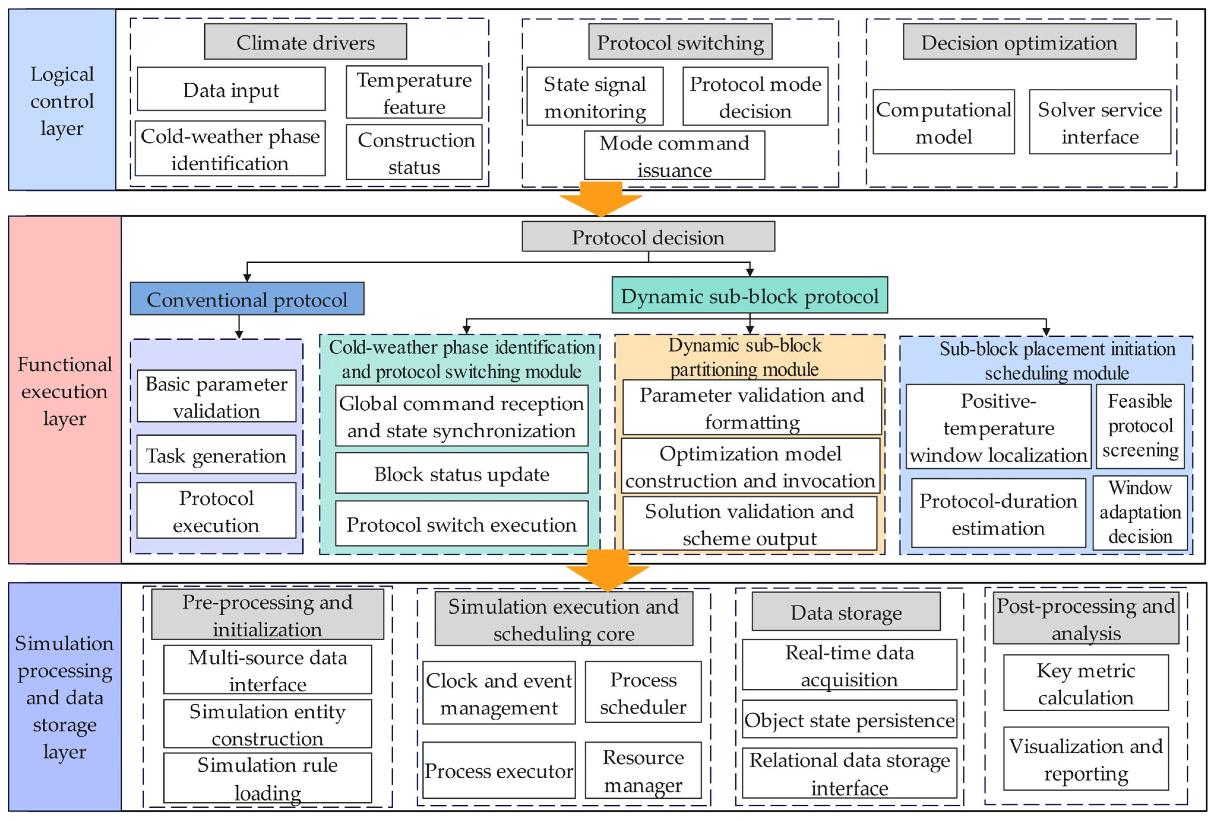
The construction system of the high arch dam is a typical dynamic system characterized by discrete states, parallel operations, complex resource contention, and multiple spatiotemporal constraints. The core of the schedule model is to simulate the entire sequence of processes, including block preparation, concrete pouring, curing, temperature control, and joint grouting, to identify various constraints and make decisions on block selection and pouring timing. Therefore, after introducing the dynamic sub-block pouring process, it is necessary to establish a schedule model that integrates a meteorological driving mechanism and process-switching logic, which enables the simulation of and schedule prediction for arch dam construction that accommodates the new process.
3.1. Overall Model Framework and Underlying Constraints
The modeling framework is based on discrete-event simulation (DES). Using a process-interaction paradigm, the simulation engine manages execution schedules by maintaining a future-event list (FEL) and a current-event list (CEL). In this architecture, each concrete block is defined as an autonomous entity. Each entity has an independent process thread, which consists of a sequence of discrete events marking the start and the end of preparation, concrete placement, and interlayer curing intervals. As the simulation progresses, system state transitions are governed by the process logic of the entities and by physical and technological constraints.
- (1)
Multi-constraint operator set
To ensure the engineering feasibility of the simulation results, the model is bound by a comprehensive constraint set covering all operational elements:
Joint grouting constraints : Follow the principles of age, temperature, and overburden compliance. That is, joint grouting can commence only after the secondary cooling age (e.g., 120 days), the secondary cooling control temperature, and the overburden height above the grouting zone have been met. After all transverse joints in this zone are closed, new growth-domain boundaries are activated. The cantilever height constraint specifically determines these boundaries.
Temporal constraint : A block must follow the rigid temporal sequence of each process, advancing in the order of block preparation, pouring, curing, formwork removal, etc. After a lower block is finished, the overlying block cannot be poured until the preparation work is complete and the minimum interlayer interval requirement is met.
Construction height difference constraint : Strictly control the maximum and minimum height differences between adjacent monoliths, the maximum construction height difference across the entire dam, and the cantilever height to satisfy temperature control, formwork erection, and dam structural-safety requirements.
Meteorological constraint : As the core trigger variable, this constraint monitors the temperature sequence in real time, driving automatic switching between the normal process and the dynamic sub-block process, and strictly enforces the temperature requirement for starting pouring during winter.
Hydration heat constraint: The heat released by cement hydration governs the temperature field of a dam and the associated control strategy. The model defines, in its miscellaneous parameters, the final adiabatic temperature rise (), the fitted temperature-rise curve parameters (n, m), the specific heat capacity (c), and the density (ρ) of the four-graded concrete blocks, from which the cumulative hydration heat per unit volume is calculated. Combined with the pipe cooling parameters in the miscellaneous temperature-control parameter set, temperature control measures are implemented.
- (2)
State transition mechanism
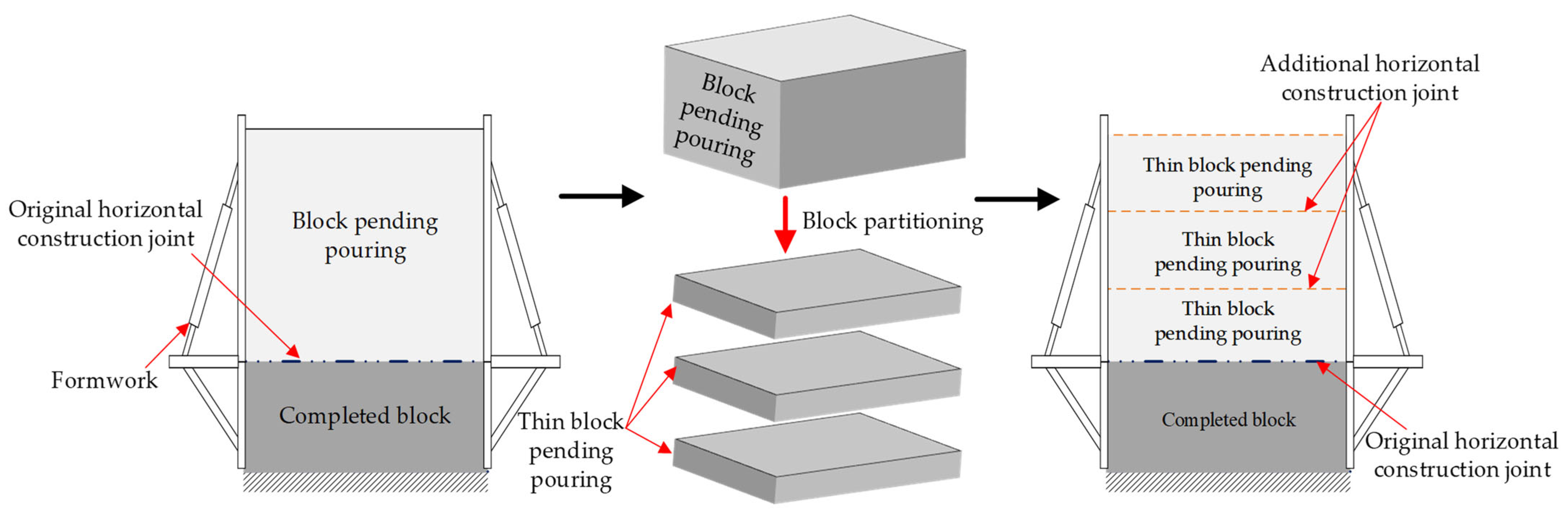
The evolution of the system state S at time step t can be expressed as the logical intersection of all active entities filtered by the above constraint set. When the system detects a low-temperature meteorological signal, it activates the dynamic sub-block decision module, dynamically adjusting the progress by redefining the block’s geometric properties (e.g., adjusting the lift thickness from H to h) and repositioning the pouring window.
When the simulation begins, the system state is set to , the simulation time to , and the target state to , with duration . Here, N represents the total number of system state changes and is a variable to be determined. In each simulation step, the event with the earliest occurrence time in the future-event list (FEL) is first moved to the current-event list (CEL). Then, the process corresponding to that entity is advanced until it is interrupted due to resource constraints or unsatisfied logical conditions. The interrupted process is removed from the CEL, and a record for its next event is created in the FEL.
Specifically, in the pouring simulation, when the system is in state
, the set of blocks waiting to be poured is extracted from the FEL. The feasible block set
is filtered based on the above spatial height difference constraints (e.g., maximum/minimum adjacent height differences, full-dam maximum height difference, cantilever height difference), temporal constraints (e.g., interlayer interval, grouting age), and pouring start conditions, as expressed in Equation (1).
For
, the system further checks the concrete supply capacity
, the availability and spatial accessibility
, respectively, of cable crane resources
, the safe distance between cable cranes
, and the cable crane pouring capacity
CCP to perform resource matching, thereby determining the feasible scheme set
, as shown in Equation (2).
Here,
is the resource-matching function, which comprehensively evaluates the match between currently available resources and the construction requirements of the candidate blocks to determine the feasible scheme set. From the feasible scheme set
, the ultimate selection is made according to the prioritization protocol. The main decision indicators include: monolith elevation, overdue waiting time, structural complexity, odd/even monolith (appearance shape control indicator), etc. It should be noted that the current model only avoids crane conflicts statically by enforcing a minimum safety separation distance, without implementing global optimization of dynamic multi-crane collisions—a simplification inherent to the model. From this feasible set,
, the ultimate selection of placement blocks is governed by a prioritization protocol. The primary decision metrics driving this selection include the current monolith elevation, accumulated idle time, structural complexity, and odd–even monolith sequencing—a critical metric utilized to control the macroscopic construction profile of the rising dam.
In Equation (3), is the quantified value of a candidate block and is the weight of each indicator. The weights, as fixed values, are not self-calibrated by the model but rather determined based on engineering experience combined with the actual management objectives of high arch dam construction and expert judgments. is the finally selected block, and is the normalized quantified value of each decision indicator.
From the perspective of project duration, it is desirable to have high pouring intensity. Therefore, the optimization objective for the pouring scheme is to maximize the overall pouring intensity, as shown in Equation (4).
Here,
is the performance indicator of the scheme,
I is the set of blocks in the planning period, and
is the total pouring intensity of the cable cranes under the scheme. Based on this, the optimal scheme
is selected. After executing the selected scheme, the simulation clock advances to
, and the system state transitions according to Equation (5):
In Equation (5), is the state transition function. This process is executed in cycles until all blocks are poured and the target state is reached.
Within the above multi-dimensional constraint framework, selecting the optimal pouring block from the feasible set to maximize construction efficiency is essentially a combinatorial optimization problem with complex constraints. For such resource allocation and conflict minimization problems, some studies have adopted optimization methods such as integer linear programming (ILP), demonstrating that they can efficiently obtain the globally optimal solution [
30]. However, ILP methods usually require linear constraints and objectives and have limited adaptability to dynamic random events. By contrast, this paper adopts the DES framework. Through process interaction and event-driven mechanisms, it can flexibly characterize nonlinear logic, such as low-temperature meteorological triggering and dynamic sub-block switching.
Climate-Driven Simulation Framework
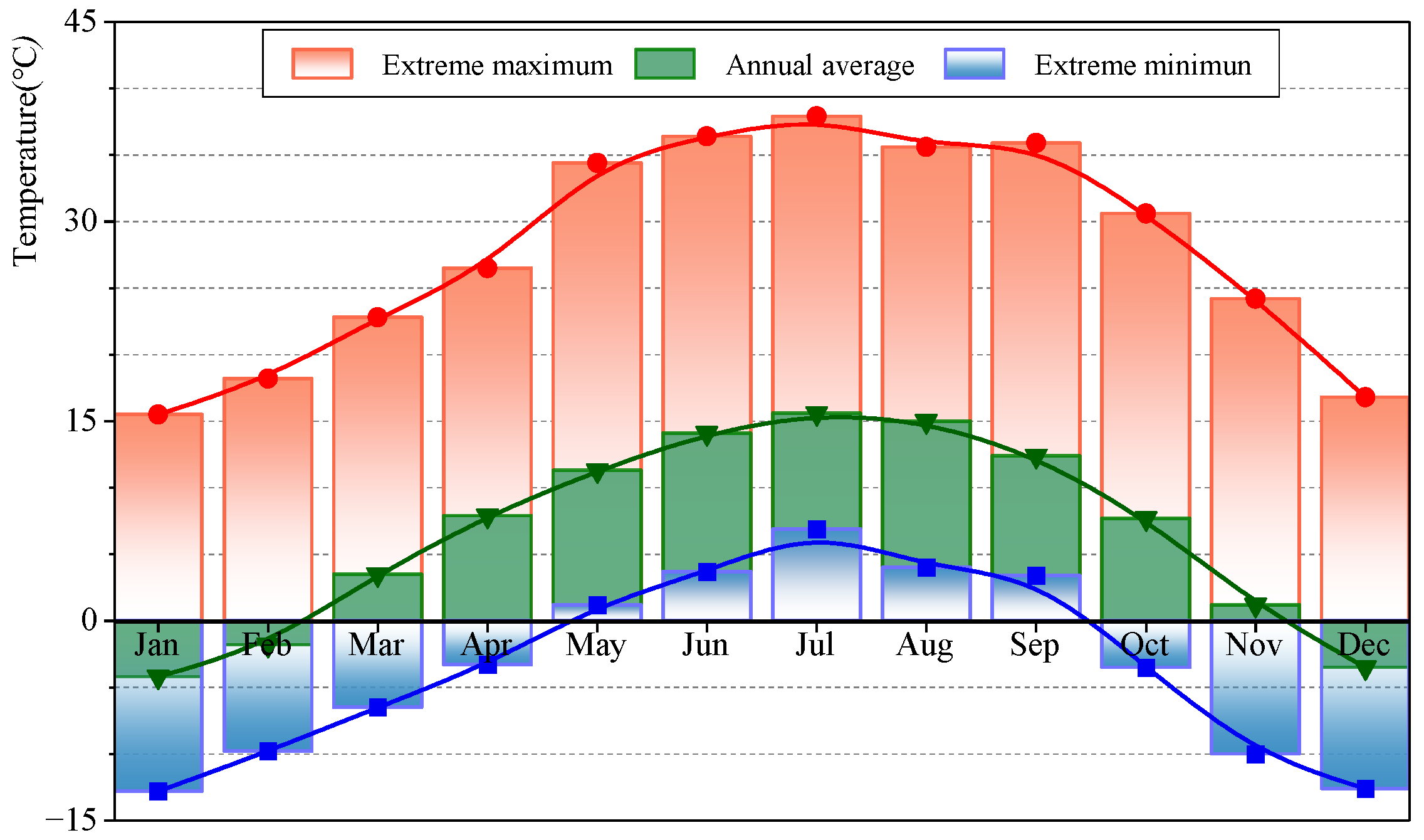
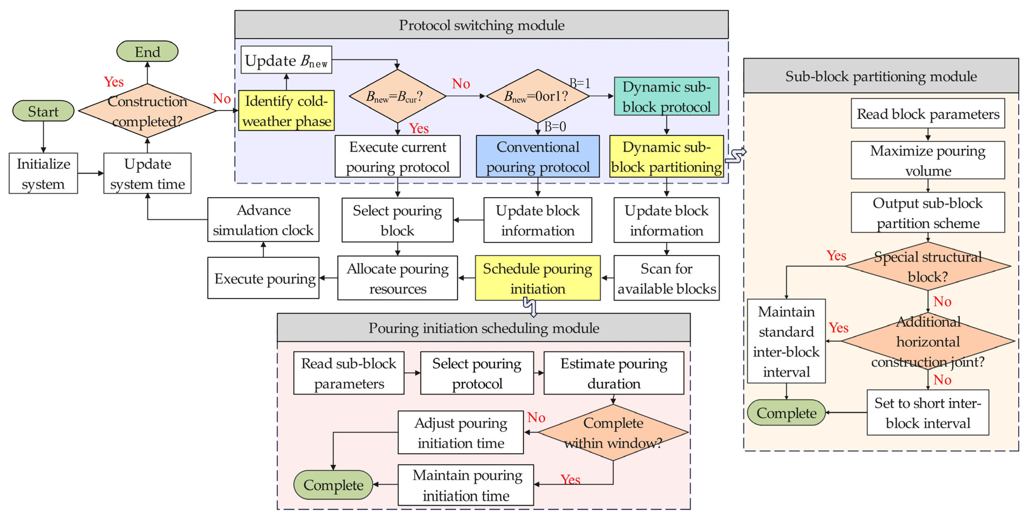
The simulation system can switch adaptively between normal mode and dynamic sub-block mode. Switching is triggered by real-time temperature data. When the daily average temperature remains stably below 5 °C for five consecutive days, the system switches to the dynamic sub-block mode. Otherwise, it switches back to the normal mode. The overall simulation process is shown in
Figure 5.
- (1)
Normal mode: The standard pouring process is executed with the standard block thickness H. Simulation events proceed cyclically in the established order: updating block status, filtering eligible blocks, selecting the optimal block, allocating resources, and, finally, completing pouring.
- (2)
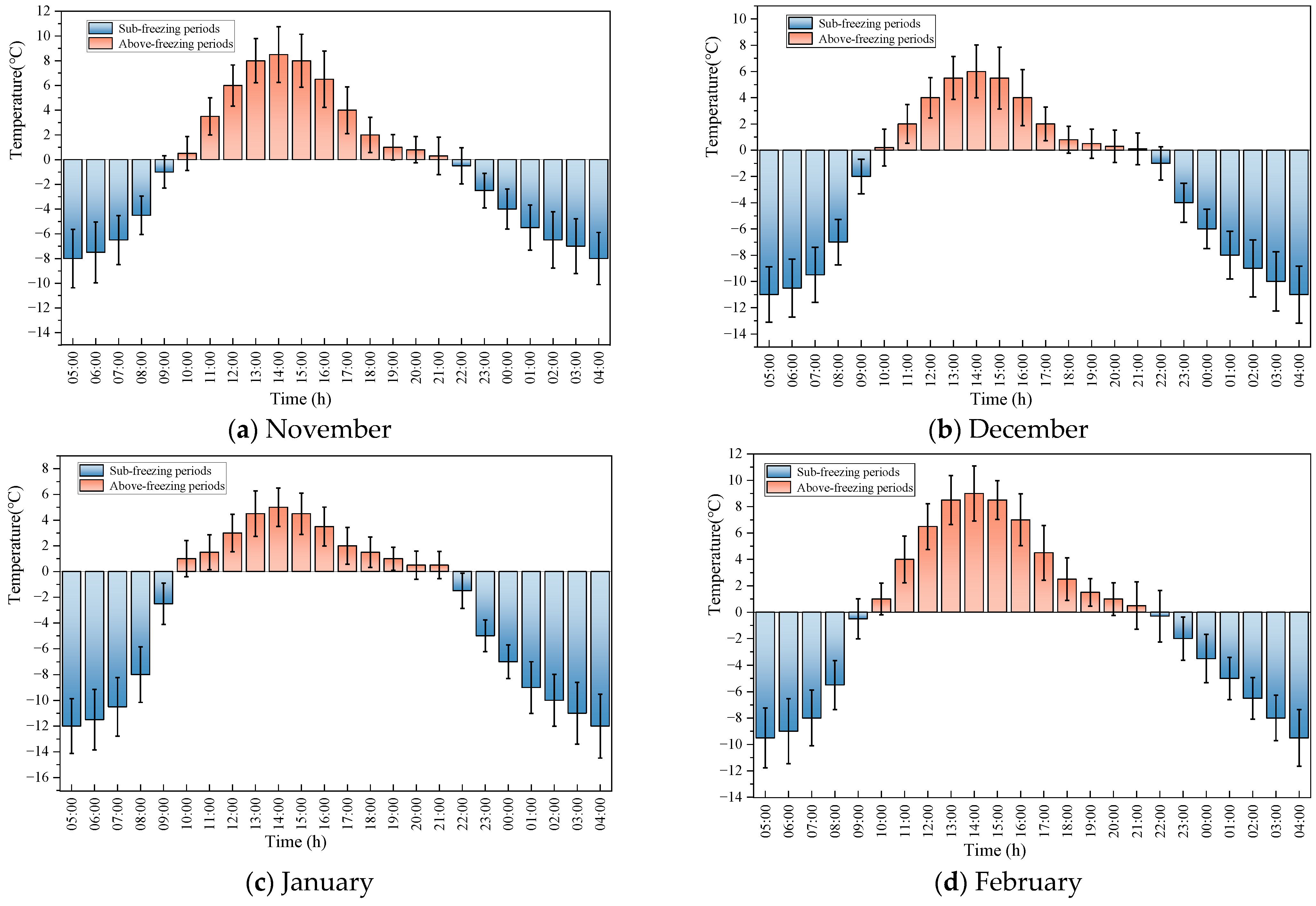
Low-temperature period: The dynamic sub-block module subdivides H into h, and the sub-block planning module ensures that operations are strictly confined within the daily positive-temperature window.
The simulation uses discrete-event time to advance. Core events include entity generation, ready for pouring, curing completion, and grouting. Processing procedures are as follows. The clock first switches to the earliest event time in the FEL, and all events at that time are moved to the CEL. Then, they are processed sequentially by type.
As for resource allocation, cable cranes adopt a two-stage strategy: availability first, then block priority. First, feasible blocks are filtered to satisfy spatial, temporal, and meteorological constraints and are scored according to Equation (3). When multiple blocks compete, the one with the higher score has priority. When crane conflicts occur, a minimum safe spacing of 15 m is maintained. Simulation terminates when all monoliths have reached the crest elevation.
Conflict resolution is incorporated under the dynamic sub-block mode. The benching method is preferentially used when a sub-block cannot be completed within the current positive-temperature window. If still infeasible, it is postponed to the next positive-temperature window. If postponement leads to abnormal intervals, the block is repartitioned (sub-block thickness reduced to ≥1.0 m) to ensure completion within the positive-temperature window.
3.2. Core Functional Modules for Dynamic Sub-Block Simulation
To enable continuous pouring during winter, the schedule simulation system based on dynamic sub-blocks incorporates three core modules: low-temperature identification and process switching, dynamic sub-block partitioning, and sub-block pouring scheduling.
3.2.1. Low-Temperature Period Identification and Strategy-Switching Module
In the simulation system, each block’s information includes the block number, bottom and top elevations, volume, spatial coordinates, concrete material zoning, and minimum interval time. The data structure is complex. During simulation, each judgment of the low-temperature period updates the block information, triggering frequent, large-scale data reads/writes and state refresh, thereby increasing the computational load. To address this issue, this module specifically designs two subroutines: low-temperature period identification and strategy switching.
- (1)
Low-temperature-period identification
A discriminant function
B is defined. After the system time is updated, it determines whether the current time falls within the low-temperature period and then updates
, as shown in Equation (6), where
indicates the dynamic sub-block pouring strategy;
indicates the normal pouring strategy.
Here,
represents the number of consecutive days with a daily average temperature threshold below 5 °C. This threshold directly follows the stipulation in the Specifications for Hydraulic Concrete Construction [
22], which requires that when the daily average temperature is continuously below 5 °C for five days, thermal insulation measures must be taken and the pouring thickness must be controlled. This is precisely the prerequisite for the dynamic sub-block strategy proposed in this paper.
- (2)
Strategy switching
This subroutine is responsible for switching the construction strategy based on the identification result. is defined as the current process value.
After the system simulation time is updated, the new discriminant state is calculated using the criterion above. The logical execution proceeds as follows:
When , it leads to a process switch. Depending on the value of , different pouring processes are triggered. If , the dynamic sub-block pouring strategy is invoked, and the block and strategy information are queried and updated. If , the normal pouring strategy is restored, with block and information queried and updated. Then, is assigned to . If , this subroutine is skipped without any update.
Through the above design, block information is updated only when , which reduces unnecessary query and computation loads.
3.2.2. Dynamic Sub-Block Partitioning Module
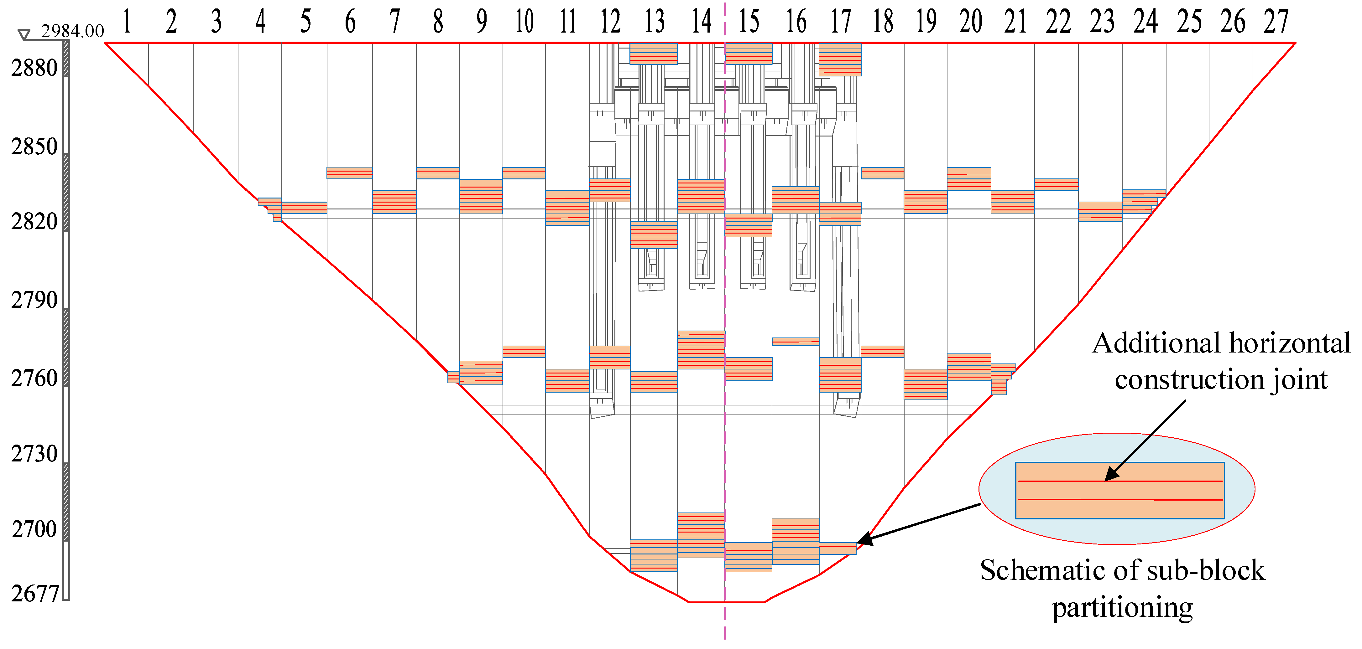
Within the discrete-event simulation framework, the dynamic sub-block partitioning module is a dedicated process triggered by the winter construction mode switch. Based on preset deterministic rules (e.g., sequential subdivision by lift thickness of 1.5 m, merging the remaining thickness into the top layer, etc.), this module generates a sub-block partitioning scheme, which is the combination of the number and thickness of sub-blocks. According to a preset interlayer interval time, the module preliminarily schedules the start time of each sub-block. The original intention of this module is to maximize the cumulative pouring volume during the cold period. This goal is not achieved through mathematical optimization but rather relies on the above rule-driven process. The generated partitioning scheme and its preliminary schedule are entered into the FEL as a new, ready sub-block, which then drives the subsequent simulation process.
In this module, the optimization target is defined as , the set of blocks scheduled within planning. Any block i in this set is a predetermined construction task that the simulation system outputs in advance according to the overall schedule. A Boolean decision variable is introduced. It is T if the j-th layer (from bottom to top) of block i is scheduled to be poured and is F otherwise. A continuous decision variable is also introduced, representing the planned thickness of the corresponding sub-block. Let be the index set of sub-block sequences for block i, and let be the estimated maximum number of sub-blocks derived from and .
After setting the decision variables, the module aims to maximize the total cumulative concrete volume
V poured over
M blocks. This design preference must be considered together with the following operational constraints (allowable pouring duration and resource availability), which can be expressed mathematically as:
In this formulation,
and
denote the base area and the total design height, respectively. The engineering codes require the minimum single-layer thickness to be
. In combination with practice, a standard reference layer thickness
is set. Within planning, the daily available positive-temperature duration is
, the number of cable cranes available is
N, and the average pouring intensity of a single crane is
q.
In Equation (8), Constraint ① ensures that the cumulative placement height of any given block strictly respects its prescribed design height. Constraint ② ensures consistency between the thickness variable and the decision variable and satisfies the minimum layer-thickness specification. If the layer is selected (), its thickness must be at least Otherwise, the thickness is forced to zero. Constraint ③ ensures that the pouring duration of all planned sub-layers does not exceed the positive-temperature window length. Within Constraint ②, priority is given to layering according to , while for special layer thicknesses, the residual thickness is handled flexibly. Its handling rules are as follows:
- (1)
Flexible Top-Layer Thickness: The top-layer thickness is allowed to vary within to accommodate non-standard residual thicknesses;
- (2)
Residual Merging: If the top-layer thickness is significantly smaller than , then no further layer is planned , and the residual thickness is merged into the current layer.
The output of this module is a set of sub-block partitioning schemes for M blocks within planning. For a given block , the output is , meaning the block will be divided into sub-blocks with corresponding thicknesses .
3.2.3. Sub-Block Initiation Scheduling Module Based on Positive-Temperature Windows
This module triggers a decision of the ready sub-block event. The process receives the sub-block entities and their initial start-time output from the dynamic sub-block partitioning module. Its core task is to match a feasible start time and pouring process for each sub-block.
Once activated, the process first performs an intensity check. Based on real-time monitoring [
31], the simulation system dynamically obtains the measured average pouring intensity of the cable crane groups and uses it to drive the process decision event. The system first matches a feasible process according to the minimum required intensity: ① If the available intensity is not less than the minimum intensity required for the horizontal layering method, the method is triggered preferentially. ② The benching method is triggered if the required intensity only meets its lower bound and the estimated pouring duration can be completed within the current positive-temperature window. ③ If none of the above methods are satisfied, the current sub-block partitioning scheme cannot fit the window. Thus, a re-planning event is generated, which feeds back into the dynamic sub-block partitioning module for scheme iteration until a feasible solution is obtained. The minimum pouring intensities required for each process are:
In Equation (9), denotes the time interval between spreading layers (h), and is the minimum pouring intensity for the horizontal layering method (m3/h). In Equation (10), is the concrete volume per spread step in the benching method (m3); is the spreading thickness (m); indicates the number of benches; L is the short side length of the block (m); and is the bucket volume (m3).
After verification, the process enters the decision stage for the start time of pouring. The initial planned start time is recorded, the final decision pair (start time and pouring process) is output, and the corresponding pouring is initiated and added to the FEL.
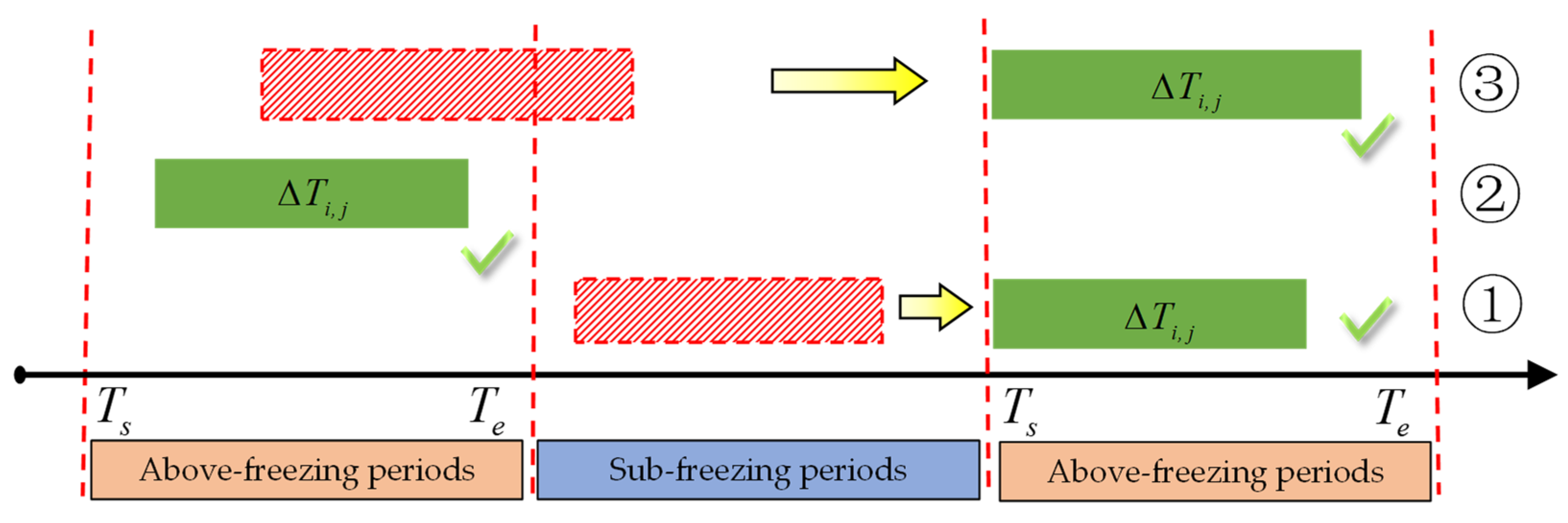
- (1)
If the initiation time
falls within a negative-temperature period, a time-domain rolling mechanism is executed to adjust
to
, the onset of the next available positive-temperature time window, which is then used as the new decision starting point. This ensures that pouring is always planned within the allowable positive-temperature window, as shown in Case ① of
Figure 6.
- (2)
When
lies within a positive-temperature window
, the simulation system selects a feasible process that satisfies the lower bound of process intensity based on the measured average pouring intensity
of the cable crane groups. It then estimates the pouring duration using Equation (11). The key criterion is whether the estimated completion time
is ahead of the window end time
. ① If a process satisfies the condition, it is selected and executed, as shown in Case ② of
Figure 6. ② If none of the feasible processes can be completed within the current window, the time-domain rolling is triggered again, postponing
to the start of the next positive-temperature window for re-planning, as shown in Case ③ of
Figure 6.
In Equation (11), is the total pouring duration for sub-block j. Considering the time incurred by equipment coordination in multi-crane operations, represents the number of crane moves, is the time per single crane move; is the block surface operation coefficient; and is the interference coefficient between cranes.




 ,
,