Frame Selection Strategies for Video Deepfake Detection: Benchmarking Accuracy and Runtime Trade-Offs

Abstract

This study evaluates frame selection during inference as an independent factor in video deepfake detection while keeping the downstream detectors fixed. We compare twelve frame selection strategies, ranging from simple temporal and quality baselines to landmark aware policies, using four validated pretrained detectors: Self-Blended Images (SBIs), Frequency-Enhanced Self-Blended Images (FSBIs), Generative Convolutional Vision Transformer (GenConViT), and GenD. The primary experiment is a complete factorial benchmark with 300 videos and five frame budgets (2, 4, 8, 16, and 32 selected frames), which provides the reference results at 32 frames. To address sample size limitations, an additional validation experiment uses a deduplicated split of 1180 Celeb-DF++ and FaceForensics++ videos, with complete results for 2, 4, and 8 selected frames and a reported subset for 16 selected frames. In the complete 300-video benchmark, 32 frames achieved the strongest average AUC, while 8 and 16 frames recovered most of the attainable performance with lower runtime. The best single validated configuration was GenD with Shot-aware sampling at 32 frames, yielding an AUC of 0.9607 and a balanced accuracy of 0.9133. The study therefore does not claim that smaller budgets universally outperform 32 frames; instead, it quantifies the tradeoff between accuracy and runtime and shows that frame selection remains a meaningful design variable under constrained inference budgets.

1. Introduction

Deepfake detectors that process individual video frames are commonly evaluated using a fixed number of frames per video, although the informativeness of individual frames is not uniform [1,2,3]. In practical video data, many frames are redundant, visually weak, or show only limited facial variation. As a result, frame selection should not be treated only as a preprocessing step, but rather as an experimental factor that can influence both classification performance and computational cost.

This issue is especially relevant for visual video deepfake detection pipelines that use pretrained image models or models that aggregate frame scores during inference [1,2,3]. Such models often rely on a relatively small subset of face frames extracted from the full clip. However, the choice of which frames are retained may affect the final decision for the video as much as the number of processed frames itself. In this context, reducing the frame budget can be valuable not only for faster inference and lower resource consumption, but also for clarifying whether the detector benefits more from temporal coverage, frame quality, motion, or geometric diversity of facial configurations.

The present study investigates this question using four validated pretrained deepfake detectors: Self-Blended Images (SBIs), Frequency-Enhanced Self-Blended Images (FSBIs), Generative Convolutional Vision Transformer (GenConViT), and Deepfake Detection that Generalizes Across Benchmarks (GenD) [1,2,3]. The models have not been retrained. Instead, the study isolates the effect of frame selection during inference by evaluating how detector performance changes when only a small number of frames is selected from each video.

To address this problem, the study compares classical frame selection heuristics with strategies that use facial landmarks. Classical baselines include uniform temporal sampling, visual diversity, quality ranking, motion sampling, Shot-aware selection, face utility scoring, TP-guided selection, and random sampling. The landmark family uses facial geometry after pose compensation to diversify the selected frames according to facial configuration rather than only visual appearance. In addition, hybrid variants combine landmark diversification with quality or motion cues.

The second contribution of the work is methodological. All detector evaluations are performed on a shared selection cache that materializes selected frames, face crops, and selection metadata before detector inference. Consequently, each detector sees the same selected frames for the same video, strategy, and frame budget. This removes repeated face extraction from the comparison loop, improves reproducibility, and makes differences between detectors easier to interpret. In this study, the cache uses visual information only, which means that audio is not used in the benchmark. The emphasis on consistent inputs and controlled detector comparison aligns with the broader calls for standardized and reproducible deepfake evaluation pipelines [4].

Unlike a purely conceptual comparison, the present manuscript is aligned with the reported benchmark outputs and explicitly separates two evidence layers. First, a complete factorial benchmark with 300 videos evaluates 12 selection strategies, 5 frame budgets (2, 4, 8, 16, and 32), and 4 validated detectors; this experiment provides the full reference at 32 frames and remains the source of all claims that compare against 32 frames. Second, an expanded validation experiment with 1180 videos evaluates the same strategy family on a deduplicated Celeb-DF++ and FaceForensics++ split, with complete coverage for the budgets of 2, 4, and 8 frames and a reported subset for 16 frames. The expanded experiment is therefore used as a robustness check for the smaller budget regimes, not as a replacement for the complete factorial benchmark with the 32 frame reference. For this reason, the manuscript emphasizes both the measured conclusions and the present experimental scope rather than presenting the study as a universal benchmark of all configured deepfake detectors.

2. State of the Art

Deepfake detection from images and videos has evolved from artifact-focused convolutional baselines toward methods that generalize better across datasets and foundation models. Early studies established both the threat model and the first practical detection baselines. Initial works showed that deepfakes are challenging for classical biometric systems and standard forensic cues [5], while compact CNN detectors such as MesoNet [6], capsule models [7], and detectors based on face warping inconsistencies [8] demonstrated that manipulated faces can often be recognized from spatial artifacts. A major milestone was FaceForensics++, which standardized evaluation and accelerated the adoption of deep learning methods for face forgery detection in common protocols [9].

A large line of work then focused on frequency information and the interaction between spatial and spectral cues. F3Net showed that DCT representations are effective for face forgery detection, especially under compression [10]. SPSL emphasized phase information as a transferable cue for detecting upsampling artifacts [11], while high-frequency feature learning further improved robustness across datasets [12]. More recent models combined spatial and frequency reasoning more explicitly, for example, through graph relation learning across content and spectrum domains [13]. These studies established frequency analysis as one of the main alternatives to detection based only on RGB input.

Another important stream addressed local inconsistencies and fine-grained facial relations. Multi-attentional deepfake detection formulated the problem as fine-grained classification and used multiple attention heads to emphasize subtle local artifacts [14]. Pair-wise self-consistency learning (PCL-I2G) modeled inconsistencies in source features within forged faces [15]. Local relation learning introduced patch-level similarity patterns and fusion of RGB and frequency evidence to capture generalized local traces [16]. Learning second-order local anomalies further improved general face forgery detection by modeling higher-order inconsistencies [17]. Transformer detectors also entered this line of work, including UIA-ViT, which learns patch inconsistency without forgery masks at the pixel level [18], and IID, which explicitly models implicit identity cues in face swapping [19].

In parallel, several methods improved generalization through reconstruction, pseudo-fake generation, or self-supervised learning. Face X-rays exploited the boundaries of blending and remain one of the most influential image methods for general detection of face forgery [20]. SBI replaced manipulation specific synthetic data with self-blended images created from pristine faces and showed strong behavior across datasets [1]. RECCE combined reconstruction and classification in an end-to-end framework to obtain common features of genuine faces [21]. SLADD used self-supervised adversarial examples to improve generalization to unseen forgeries [22]. More recent work focused on training continued in this direction by revisiting whether deepfake data are strictly necessary during training [23] and by enriching pseudo-fake generation in the frequency domain through FreqBlender [24].

Recent state-of-the-art research has increasingly emphasized generalization across datasets and robustness at the video level. AltFreezing addressed the imbalance between spatial and temporal evidence in video face forgery detection [25]. UCF proposed uncovering common forgery features that transfer better across benchmarks [26], while SeeABLE framed detection as a bounded one class problem for out of distribution detection using soft discrepancies [27]. Identity leakage was later identified as a major obstacle to generalization in binary deepfake classifiers [28]. LSDA expanded the effective forgery space by augmentation in latent space [29], and StyleGRU-style modeling of latent flow showed that temporal abnormalities in style latents are useful for generalization at the video level [30]. At the same time, detectors based on CLIP and transformers became increasingly prominent, including Forensics Adapter [31], GenConViT [2], and GenD, which demonstrated strong performance across benchmarks with a parameter efficient CLIP design [3].

Benchmarking and evaluation methodologies have also become a central part of the field. DeepfakeBench unified datasets, preprocessing, model implementations, and evaluation protocols for a large set of detectors [4]. DF40 also highlighted the need for more realistic and next generation evaluation settings [32]. These benchmark efforts made it easier to compare detectors fairly, but they also revealed that most progress has been driven by detector architecture, training objectives, and strategies for generalization across datasets rather than by systematic analysis of frame selection during inference.

Recent work on frame selection has started to address this gap more directly. Dincer et al. proposed a deepfake video detector in which frames are selected using pupil and golden ratio facial cues instead of random frame choice [33]. Hu et al. later proposed ADA-FInfer, an adaptive method for frame selection and face representation inference that uses optical flow evidence to select frames for deepfake detection in videos with high visual quality [34]. These studies support the view that frame choice is not a neutral preprocessing detail. However, they mainly introduce detector specific pipelines, whereas the present work treats the selection policy itself as the controlled benchmark variable and evaluates multiple strategies, frame budgets, and fixed downstream detectors under a shared cache protocol.

This observation is particularly relevant for the present study. Many successful deepfake detectors operate on images or individual frames and ultimately use a fixed number of selected facial crops before aggregating frame scores into a score for the full video [1,2,3,9,25]. However, the literature has devoted much more attention to designing stronger detectors than to studying which frames should be selected under a strict inference budget. In this sense, the current work complements the existing state of the art by shifting the focus from detector design to the efficiency and informativeness of frame selection itself while keeping the downstream detectors fixed.

3. Materials and Methods

3.1. Study Configuration

The study considers binary classification at the video level, where each input video is assigned to either the real or deepfake class using visual information only. The revised experimental design contains two complementary parts. The first part is the complete factorial benchmark used for the main reference at 32 frames: 300 videos, 12 frame selection strategies, 5 frame budgets (2, 4, 8, 16, and 32 selected frames per video), and 4 validated detectors (SBI, FSBI, GenConViT, and GenD). The second part is a larger validation experiment over 1180 deduplicated videos from Celeb-DF++ and FaceForensics++. This larger validation reports the complete grids for 2, 4, and 8 frames for all 4 detectors and a reported subset for 16 frames consisting of the complete SBI and FSBI strategy grids together with selected GenD and GenConViT configurations. This design keeps the complete comparison at 32 frames in the primary benchmark while directly addressing whether the trends for smaller budgets are stable on a larger and less redundant evaluation set.

Table 1. Experimental evidence layers used in the revised manuscript.

Experiment	Scope	Frame Budgets	Role in the Manuscript
Complete factorial benchmark	300 videos; 12 strategies; 4 detectors	2, 4, 8, 16, 32	Primary reference for detector, strategy, runtime, and delta analyses.
Expanded validation benchmark	1180 deduplicated videos; 12 strategies; four detectors	2, 4, 8 complete; 16 subset	Robustness check on a larger Celeb-DF++ and FaceForensics++ split for smaller budget trends.

summarizes the role of the two evidence layers in the revised manuscript.

Let v denote a video and let $\mathcal{C}\left(v\right)=\{x_1,x_2,\dots ,x_N\}$ denote its candidate face frames after preprocessing. For a frame selection strategy $\pi$ and frame budget $B\in \{2,4,8,16,32\}$, a subset

$${\mathcal{S}}_{\pi ,B}\left(v\right)\subseteq \mathcal{C}\left(v\right),\left|{\mathcal{S}}_{\pi ,B}\left(v\right)\right|=B$$

(1)

is selected for downstream inference. The same subset is then reused across all detectors evaluated under that video, strategy, and budget condition.

3.2. Datasets

The complete factorial benchmark with 300 videos was conducted using three public deepfake benchmarks: FaceForensics++, Celeb-DF-v2, and Celeb-DF++. These datasets were selected because they represent different levels of manipulation realism, dataset scale, and evaluation difficulty.

FaceForensics++ is one of the most widely used benchmarks in face forgery detection and includes pristine and manipulated videos generated by several face manipulation methods [9]. It provides a standard experimental setting and remains an important reference dataset in the field.

Celeb-DF-v2 was introduced to provide more realistic and visually convincing deepfake videos with fewer obvious visual artifacts than previous datasets [35]. As a result, it is commonly used to evaluate whether detectors remain effective in more challenging and realistic conditions.

Celeb-DF++ is a more recent large benchmark designed to support the evaluation of generalizable deepfake detection methods [36]. It extends the benchmark landscape to more diverse and difficult testing scenarios, making it especially relevant for studies focused on robustness and transferability.

Together, these datasets provide a suitable basis for analyzing whether reduced frame budgets and different frame selection strategies preserve sufficient discriminative information across deepfake benchmarks of varying difficulty. For the expanded validation experiment, Celeb-DF++ and FaceForensics++ were used after deduplication. Celeb-DF-v2 was not treated as an independent source in this larger split because the available manifests contained overlapping files with the Celeb-DF++ data source. The expanded split therefore emphasizes sample size and source separation while avoiding duplicate videos across dataset manifests.

3.3. Compared Detectors

Four pretrained deepfake detectors were included in the present quantitative comparison: SBI, FSBI, GenConViT, and GenD. The purpose of the study is not to retrain these models but to evaluate how strongly their behavior at the video level depends on frame budget and frame selection policy. All detector weights were kept fixed during the experiments. Thus, the observed differences can be attributed to frame selection during inference rather than to changes in optimization or training data. Additional detectors were explored during implementation, but they are not used as evidence in this manuscript unless complete validated outputs are available. This avoids drawing conclusions from unvalidated baselines.

Table 2. Validated pretrained detectors used in the reported benchmark.

Detector	Core Idea	Use in This Study
SBI	Self-Blended Images detector trained to identify face forgery artifacts from synthetic self blending examples.	Fixed image detector applied to the selected face crops; video scores are obtained by mean aggregation.
FSBI	Frequency-enhanced extension of the self-blended image family, emphasizing spatial and frequency cues for forgery detection.	Fixed image detector applied under the same cache of selected frames as the other models.
GenConViT	Hybrid convolutional and vision transformer detector designed to combine local visual evidence with transformer style representation learning.	Fixed frame detector evaluated on identical selected crops for each strategy and budget.
GenD	CLIP-based detector designed for stronger generalization across benchmarks in deepfake detection.	Fixed frame detector; it provides the strongest average AUC in the completed benchmark with 300 videos.

summarizes the validated detector set used for the reported quantitative results.

3.4. Shared Selection Cache

A dedicated preparation stage materializes selected frames, selection manifests, and face crops before the detector benchmark. For each video, a candidate pool is sampled from the original clip. Uniform sampling uses the requested frame budget directly, whereas the other strategies inspect a larger candidate pool capped by the configured maximum number of candidate frames. Faces are detected with a RetinaFace detector, the primary face is selected by face area, and retained faces are cropped from the detected bounding boxes and resized to 380 × 380 pixels for the shared cache used by the SBI/FSBI pipeline. The selection manifest stores the video path, label, source metadata, selected frame indices, strategy, budget, face count information, quality and motion descriptors, and metadata derived from landmarks where available. Optionally, selected face tensors are also materialized as a reusable archive.

This design enables all detectors to operate on the same prepared visual inputs and avoids repeated frame extraction inside the evaluation loop. If no usable face is found in the candidate pool, the corresponding combination of video, strategy, and budget is marked as unusable rather than silently replaced with unrelated frames. The current cache uses visual information only, so audio streams are not used even if the source video originally contains them.

For the complete benchmark with 300 videos, the prepared cache contains 18,000 selection rows across videos, strategies, and budgets. The benchmark manifest contributes 100 videos from each source benchmark (Celeb-DF-v2, Celeb-DF++, and FaceForensics++), with each source balanced to 50 real and 50 fake clips. Across the five frame budgets, the benchmark therefore materializes 223,200 selected frame positions before detector inference. For the expanded validation experiment with 1180 videos, the same cache protocol is reused on the deduplicated Celeb-DF++ and FaceForensics++ split for the complete grids at 2, 4, and 8 frames and for the reported subset at 16 frames. The expanded run is used to strengthen the sample size argument for the smaller budget regimes, while the complete run with 300 videos remains the only experiment used for direct comparisons against 32 frames. These counts reflect the controlled benchmark inputs used in the present experiments.

3.5. Frame Selection Strategies

The study compares twelve frame selection strategies that range from simple baselines to methods that use landmarks. Their role is to choose a subset of frames that is maximally informative under a strict frame budget.

Table 3. Frame selection strategies used in the study.

Strategy	Description
Uniform	Samples frames at roughly equal temporal spacing and serves as the main simple baseline.
Diversity	Chooses frames that are visually most different from one another to avoid near duplicates.
Quality	Ranks candidate face crops with an image quality model that does not require a reference image and keeps the best scoring ones.
Motion	Favors frames with stronger temporal change, where manipulations may be more visible.
Shot-aware	Spreads selected frames across segments that resemble shots to avoid collapsing onto a single local scene.
Face utility	Combines face size, centeredness, sharpness, and exposure into a score for face usefulness in this task.
TP-guided	Uses supportive evidence from the prototype detector to prefer frames that look more helpful for true positive detection.
Landmark diversity	After pose normalization, prefers frames whose landmark geometry differs the most.
Landmark cluster	Clusters landmark configurations after pose compensation and picks representatives from different geometric groups.
Landmark + quality	First diversifies by landmark clusters, then keeps the representative with the best quality inside each cluster.
Landmark + motion	First diversifies by landmark geometry, then prioritizes representatives with stronger temporal change.
Random	Draws frames randomly and acts as a sanity check baseline.

summarizes the compared strategies.

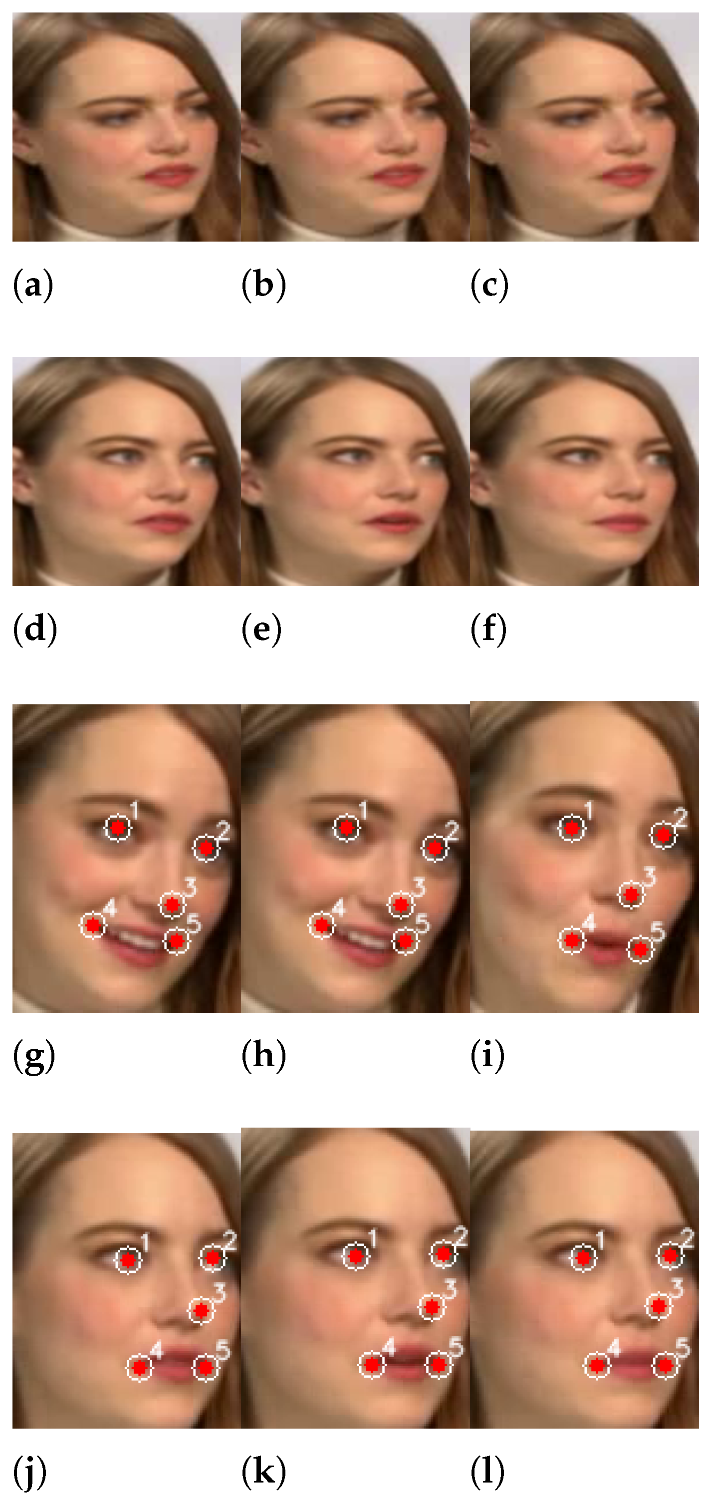
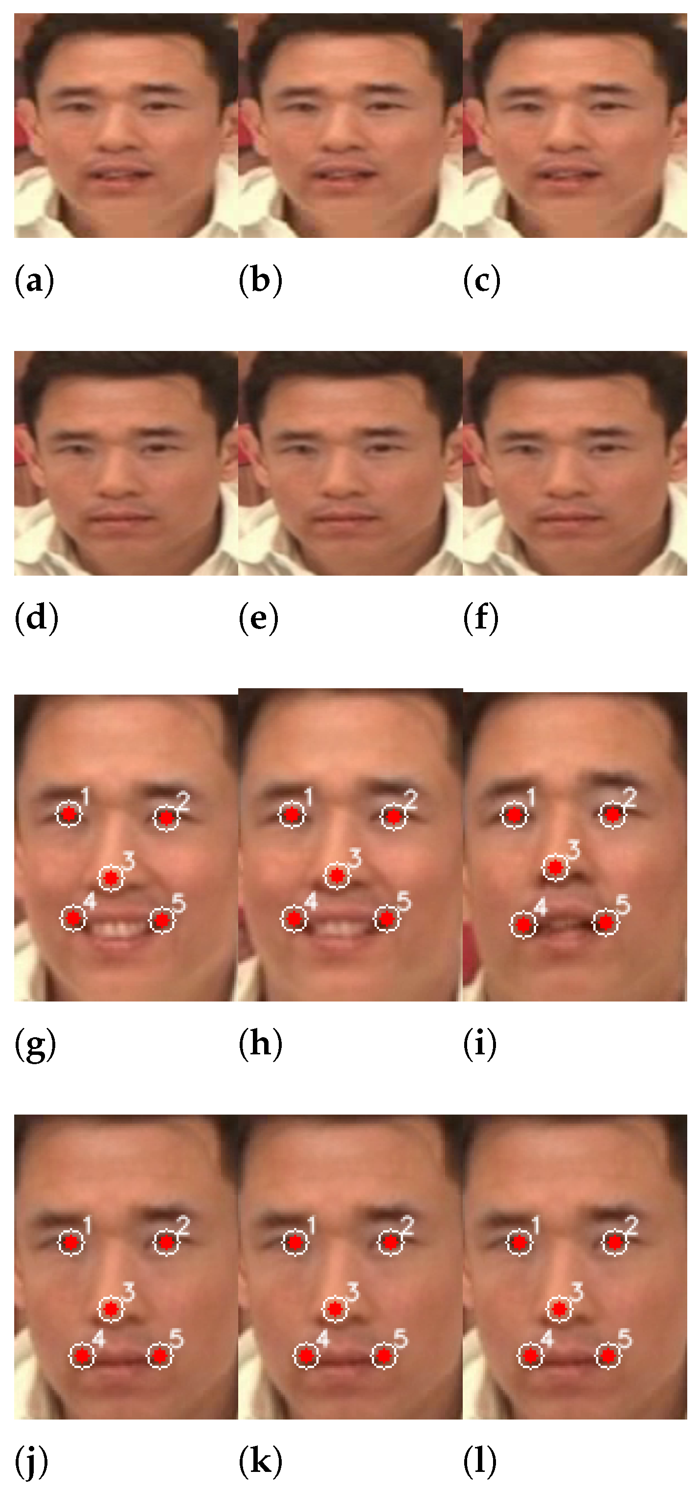
Besides the aggregate quantitative summaries reported later in Section 4, representative qualitative frame grids are retained here to show what the selection policies actually return on individual videos. These visual examples were generated from the same frame selection pipeline and help illustrate how different strategies emphasize temporal coverage, image quality, and diversity in facial geometry on concrete clips. They are included as examples for intuition rather than as separate evidence beyond the completed benchmark with 300 videos. The quantitative benchmark itself uses all five budgets, including two selected frames. For readability, the qualitative grids show a representative subset of benchmark budgets (4, 8, and 16 frames) rather than every tested budget.

Figure 1 and Figure 2 provide qualitative examples for the same 4 selection policies across representative budgets of 4, 8, and 16 frames; the complete quantitative benchmark still uses the full grid with 2, 4, 8, 16, and 32 selected frames. These strategies can be interpreted as using different notions of frame informativeness. Uniform and random sampling primarily control temporal coverage. Quality and face utility methods prioritize technically usable face crops. Motion and Shot-aware strategies emphasize temporal events and scene variation. The landmark strategies instead focus on geometric diversity of facial configuration, which is especially relevant when a detector operates on individual face frames and may benefit from seeing a broader range of expressions, mouth shapes, or other facial deformations.

3.6. Video Level Aggregation

For a detector $f_m(·)$, each selected frame $x_i\in {\mathcal{S}}_{\pi ,B}\left(v\right)$ yields a frame fake score

$$p_i=f_m\left(x_i\right).$$

(2)

The video score is computed by averaging the fake scores of the selected frames,

$$\widehat{p}\left(v\right)={\displaystyle \frac{1}{|{\mathcal{S}}_{\pi ,B}\left(v\right)|}}\sum _{x_i\in {\mathcal{S}}_{\pi ,B}\left(v\right)}{p}_i.$$

(3)

This aggregation rule is independent of the detector and keeps comparisons across frame budgets direct. It also ensures that changes in the video score are attributable to the selected frames and detector outputs rather than to temporal aggregation layers specific to a detector.

3.7. Evaluation Protocol

The present quantitative analysis focuses primarily on the frame mean AUC because it compares ranking behavior across frame selection strategies without fixing a threshold for deployment. Balanced accuracy is also reported for the best validated configuration of each detector, strategy, and budget. Precision, recall, F1 score, false-positive rate at fixed sensitivity, and calibration metrics are relevant for deployment, but they depend on operating thresholds and are therefore treated as complementary operational metrics rather than the main benchmark objective. The revision also adds validation outputs from a larger sample for the complete grids at 2, 4, and 8 frames and for a reported subset at 16 frames. The benchmark with 300 videos and the validation with 1180 videos are intentionally not pooled into a single number: the former provides the complete reference at 32 frames, while the latter tests whether the interpretation for smaller budgets remains plausible on a larger deduplicated sample. The current manuscript should therefore be interpreted as a controlled comparison of frame selection policies under a fixed set of validated detectors, rather than as a final ranking across all detector architectures that were considered during implementation.

4. Results

4.1. Overall Benchmark Summary

The primary quantitative results are based on the completed factorial benchmark with 300 videos and focus on frame mean AUC as the main summary metric. This complete experiment remains necessary because it includes the full reference at 32 frames for all 12 strategies and all four validated detectors. Among the four validated detectors, GenD achieved the strongest average performance at the detector level, with a mean frame mean AUC of 0.9464. GenConViT followed with a mean AUC of 0.9247, while FSBI and SBI reached mean AUC values of 0.8953 and 0.8935, respectively. These results indicate that the detector ranking remains clearly separated even when all models are evaluated under the same shared frame selection cache and reduced budget inference protocol. The expanded validation with 1180 videos is used to strengthen the interpretation of the smaller budget operating points rather than to replace the complete factorial benchmark with 32 frames.

Table 4. Mean AUC by frame selection strategy. Bold formatting indicates the best value in the table.

Category	Strategy	Mean AUC
Heuristic baseline	Uniform	0.9109
Heuristic baseline	Diversity	0.9121
Heuristic baseline	Quality	0.9191
Heuristic baseline	Face utility	0.9141
Heuristic baseline	Random	0.9140
Heuristic baseline	Shot-aware	0.9190
Heuristic baseline	TP-guided	0.9147
Heuristic baseline	Motion	0.9084
Landmark	Landmark cluster	0.9183
Landmark	Landmark + quality	0.9197
Landmark	Landmark diversity	0.9143
Landmark	Landmark + motion	0.9156

summarizes the average frame mean AUC obtained by each frame selection strategy on the validated detectors.

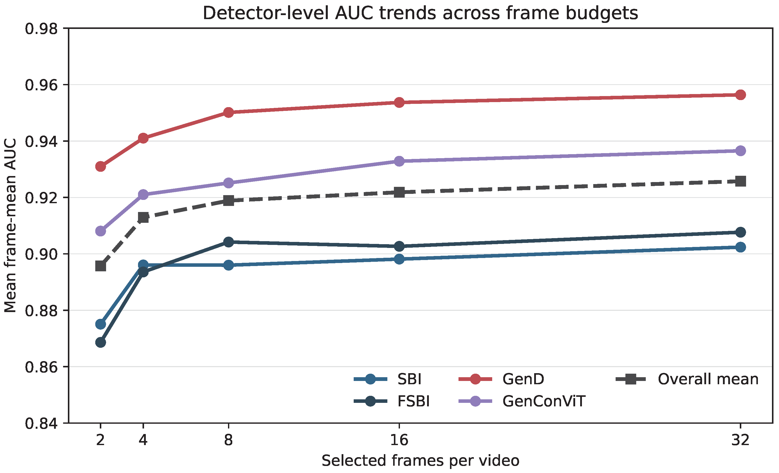
At the frame budget level, the strongest average operating point across the validated detectors was 32 selected frames, with a mean frame AUC of 0.9257. The remaining budgets followed a consistent ascending order: 16 frames reached 0.9218, 8 frames reached 0.9189, 4 frames reached 0.9129, and 2 frames reached 0.8957. Thus, the current benchmark does not show a reversal at higher frame budgets; however, the improvement from 8 to 32 frames is modest compared with the jump from 2 to 8 frames, which indicates diminishing returns rather than a strict need for dense frame usage.

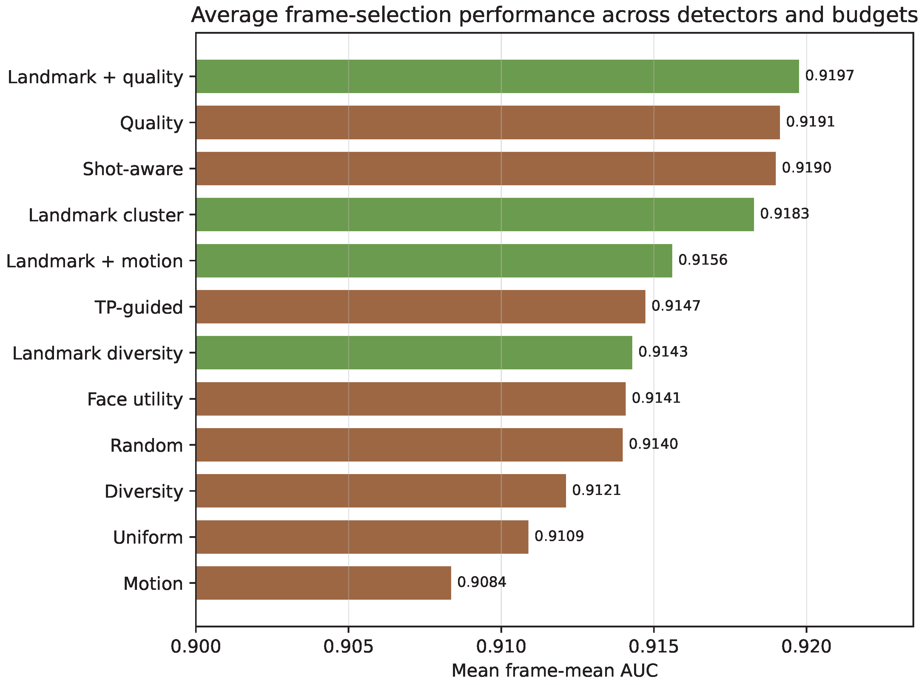
At the level of the selection strategy, the best average performance was obtained by Landmark + quality, which reached a mean frame AUC of 0.9197. The next strongest strategies were Quality (0.9191), Shot-aware (0.9190), and Landmark cluster (0.9183). The weakest average strategy in the current validated subset was Motion, with a mean AUC of 0.9084. The gap between the best landmark strategy and the best heuristic strategies is therefore small but persistent, which suggests that geometric diversification is useful in the completed benchmark, while quality heuristics remain nearly as strong. Figure 3 visualizes this ranking across the validated detector and budget configurations.

4.2. Best Configurations for Each Detector

Although landmark methods were strongest on average across validated detectors, the best configuration still depended on the detector.

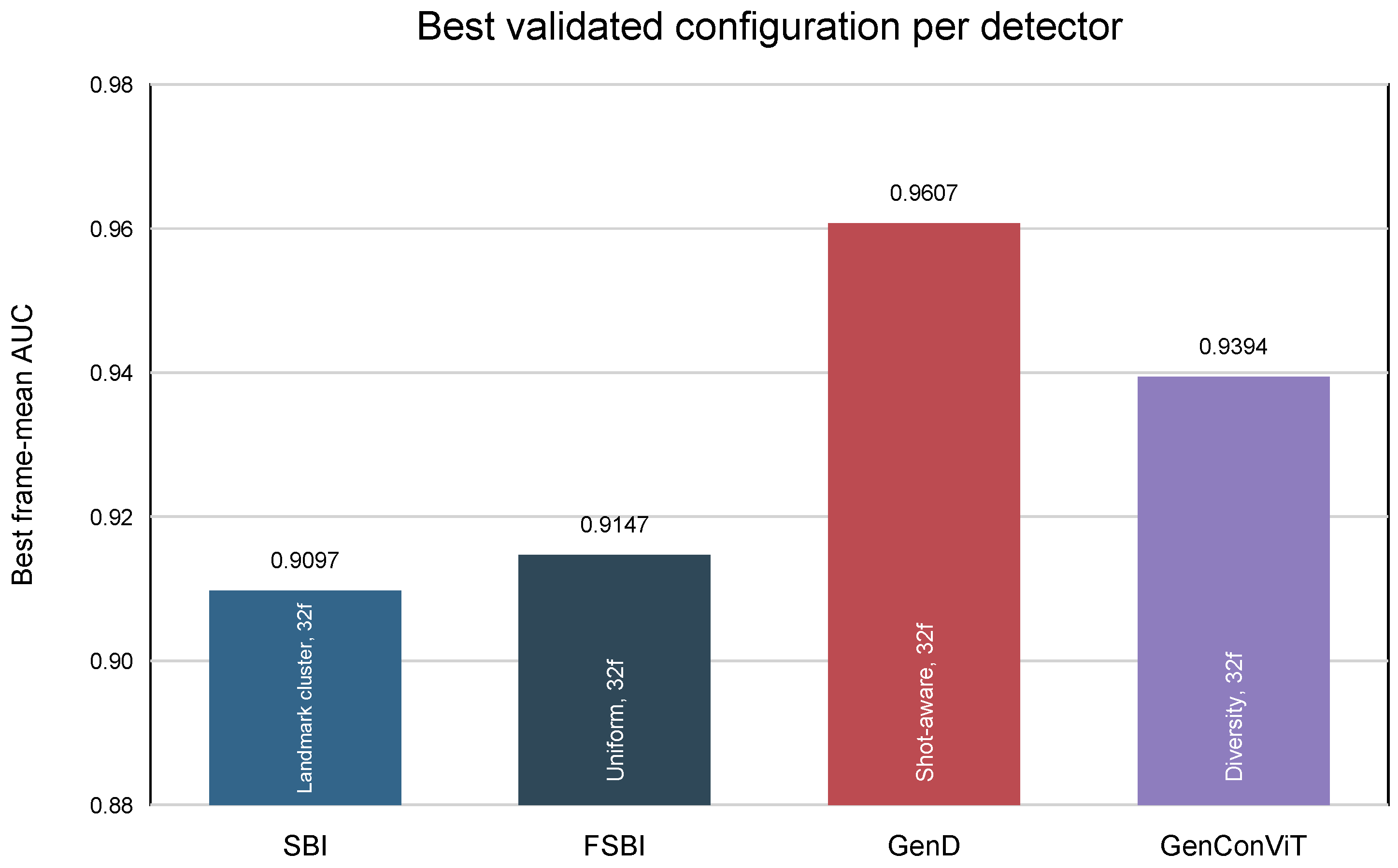
For GenConViT, the best validated configuration was Diversity with 32 selected frames, yielding an AUC of 0.9394 and a balanced accuracy of 0.7367. This result suggests that the model benefits from strong appearance diversity once the frame budget is allowed to increase toward larger budgets.

For GenD, the best validated configuration was Shot-aware with 32 selected frames, yielding an AUC of 0.9607 and a balanced accuracy of 0.9133. This is the strongest single-frame mean result among the validated detectors and indicates that the model benefits from a broader temporal spread once the budget is large enough to cover multiple local segments.

For FSBI, the best validated configuration was Uniform with 32 selected frames, producing an AUC of 0.9147 and a balanced accuracy of 0.8467. The frequency enhanced variant therefore closed most of the gap between SBI and the stronger CLIP style detectors, but still benefited most from the largest tested frame budget.

For SBI, the best validated configuration was the Landmark cluster with 32 selected frames, yielding an AUC of 0.9097 and a balanced accuracy of 0.8533. Compared with the other detectors, SBI remained the weakest average detector overall, yet it still crossed the 0.90 AUC mark when paired with a landmark strategy at the largest tested budget.

Table 5. Best validated detector configurations.

Detector	Best Strategy	Frames	AUC	Balanced Accuracy
GenD	Shot-aware	32	0.9607	0.9133
GenConViT	Diversity	32	0.9394	0.7367
FSBI	Uniform	32	0.9147	0.8467
SBI	Landmark cluster	32	0.9097	0.8533

summarizes the best validated configuration for each detector.

4.3. Effect of Frame Budget

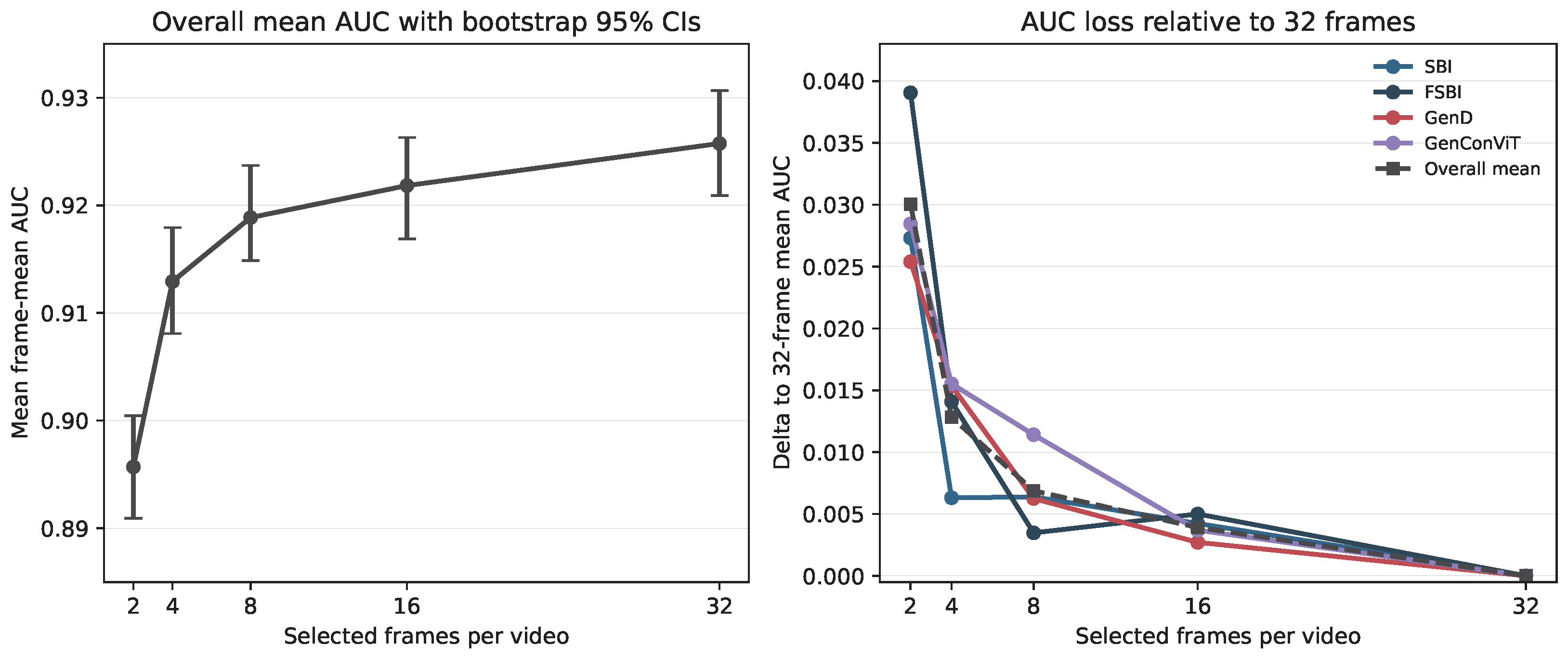
The average AUC trends for each detector across frame budgets showed a consistent upward pattern. GenConViT reached mean AUC values of 0.9081, 0.9210, 0.9251, 0.9329, and 0.9365 for 2, 4, 8, 16, and 32 frames, respectively. GenD reached 0.9310, 0.9410, 0.9501, 0.9537, and 0.9564. FSBI reached 0.8686, 0.8936, 0.9042, 0.9027, and 0.9077, while SBI reached 0.8751, 0.8961, 0.8960, 0.8981, and 0.9024. Thus, all 4 validated detectors benefited from larger frame budgets, but the gains became progressively smaller beyond 8 or 16 frames. This finding is important from a computational perspective because it shows that the budget of 32 frames is strongest in absolute terms, while smaller budgets still retain most of the achievable AUC. Figure 4 shows these budget trends for each detector and for the overall mean.

To test whether the small gaps between the higher budgets reflect a stable tendency rather than noise in a single aggregate table, a bootstrap analysis was performed directly on the prediction files at the video level for the 48 validated combinations of detector and strategy available at each budget. The resulting 95% confidence intervals for the overall mean AUC were 0.9149–0.9237 at 8 frames, 0.9169–0.9263 at 16 frames, and 0.9209–0.9307 at 32 frames. These intervals overlap substantially, which supports the interpretation that the completed benchmark exhibits diminishing returns rather than a sharp transition between the higher budgets.

A complementary analysis of the AUC loss relative to 32 frames makes the same point from the detector perspective. Relative to the baseline at 32 frames, the overall mean AUC loss is only 0.0069 at 8 frames and 0.0039 at 16 frames. The largest drop from 8 to 32 frames is observed for GenConViT (0.0114), whereas FSBI loses only 0.0035 on average. Thus, the additional gains above 8 or 16 frames are real but depend on the detector and remain comparatively small. Figure 5 combines the bootstrap confidence intervals with this loss relative to 32 frames.

4.4. Expanded Validation on the 1180 Video Split

The larger deduplicated validation split was used as a sample size robustness check for the interpretation of smaller budgets.

Table 6. Expanded validation summary for 1180 videos.

Detector	2f Mean AUC	4f Mean AUC	8f Mean AUC	16f Mean AUC	Best Reported Configuration at 16f
SBI	0.8395	0.8501	0.8526	0.8543 (12)	Quality, AUC 0.8631
FSBI	0.8414	0.8509	0.8585	0.8585 (12)	Quality, AUC 0.8722
GenD	0.9070	0.9161	0.9203	0.9220 (10)	Landmark + quality, AUC 0.9282
GenConViT	0.8491	0.8679	0.8757	0.8822 (6)	Uniform, AUC 0.8848

summarizes the mean AUC values obtained for each detector on this split with 1180 videos. The columns for 2, 4, and 8 frames correspond to complete grids with all 12 strategies for each detector. The column for 16 frames reports the subset available for the revised analysis: complete grids with 12 strategies for SBI and FSBI, 10 GenD configurations, and 6 selected GenConViT configurations.

The complete validation grids for 2, 4, and 8 frames show the same general trend as the primary benchmark: increasing the budget from 2 to 8 frames improves the mean AUC for every detector. The reported subset for 16 frames remains consistent with the diminishing returns interpretation. SBI and FSBI are nearly saturated between 8 and 16 frames on the larger split, whereas GenD and GenConViT continue to improve modestly in the reported configurations at 16 frames. This larger validation is therefore used to support the robustness of the mid budget conclusion, while the complete benchmark with 300 videos remains the source of all direct comparisons against the reference at 32 frames.

4.5. Selection Stage Runtime

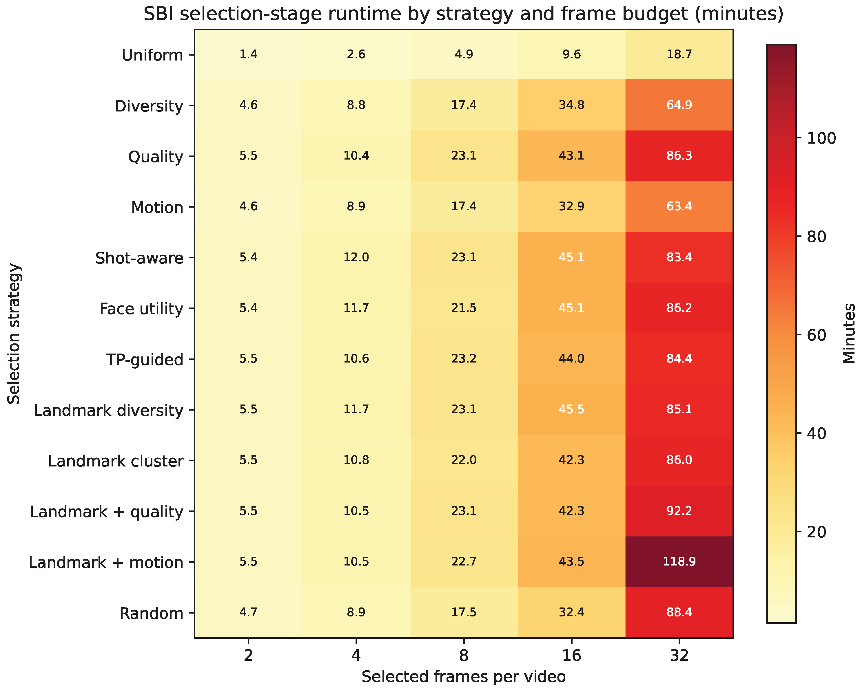
The completed benchmark also preserved wall clock information about the shared SBI selection stage. All wall clock timings reported in this section were obtained on the same server equipped with an NVIDIA H100 NVL GPU (95.8 GB VRAM), an Intel Xeon Gold 6548Y+ CPU (16 cores), and 125 GB of system memory, running Ubuntu 24.04.2 LTS with PyTorch 2.5.1 and CUDA 12.4. Consequently, the absolute runtimes should be interpreted as dependent on the hardware, whereas the relative comparisons remain directly comparable within this benchmark. The entire benchmark with 300 videos required 189,936.7 s of wall clock time from start to summary generation, or approximately 52.8 h. At a finer level, the SBI runtime logs for each strategy show that the selection stage scales sharply with the frame budget. Averaged across the 12 strategies, the total selection stage runtime increased from 295.7 s at 2 frames to 587.8 s at 4 frames, 1195.0 s at 8 frames, 2303.1 s at 16 frames, and 4789.5 s at 32 frames.

This runtime view helps to interpret the practical meaning of the AUC trends. Relative to the setting with 32 frames, the budget of 8 frames already recovers about 99.3% of the mean AUC while using only about 25% of the average recorded SBI selection runtime. The budget of 16 frames recovers about 99.6% of the mean AUC while using about 48% of that runtime. Therefore, although 32 frames remain strongest in absolute terms, the smaller mid range budgets remain attractive operating points for efficiency.

Within the runtime matrix, Uniform remains the cheapest strategy at every budget, while the more complex hybrid and guided policies become progressively more expensive as the budget grows. At 32 frames, for example, Uniform required 1124.6 s, whereas Landmark + motion reached 7133.4 s and Landmark + quality reached 5531.4 s. The timing logs are dominated by prototype generation; the recorded evaluation overhead in these SBI runtime files remained negligible by comparison. Figure 6 reports the corresponding runtime matrix in minutes.

4.6. Strategy Cost and Benefit at 32 Frames

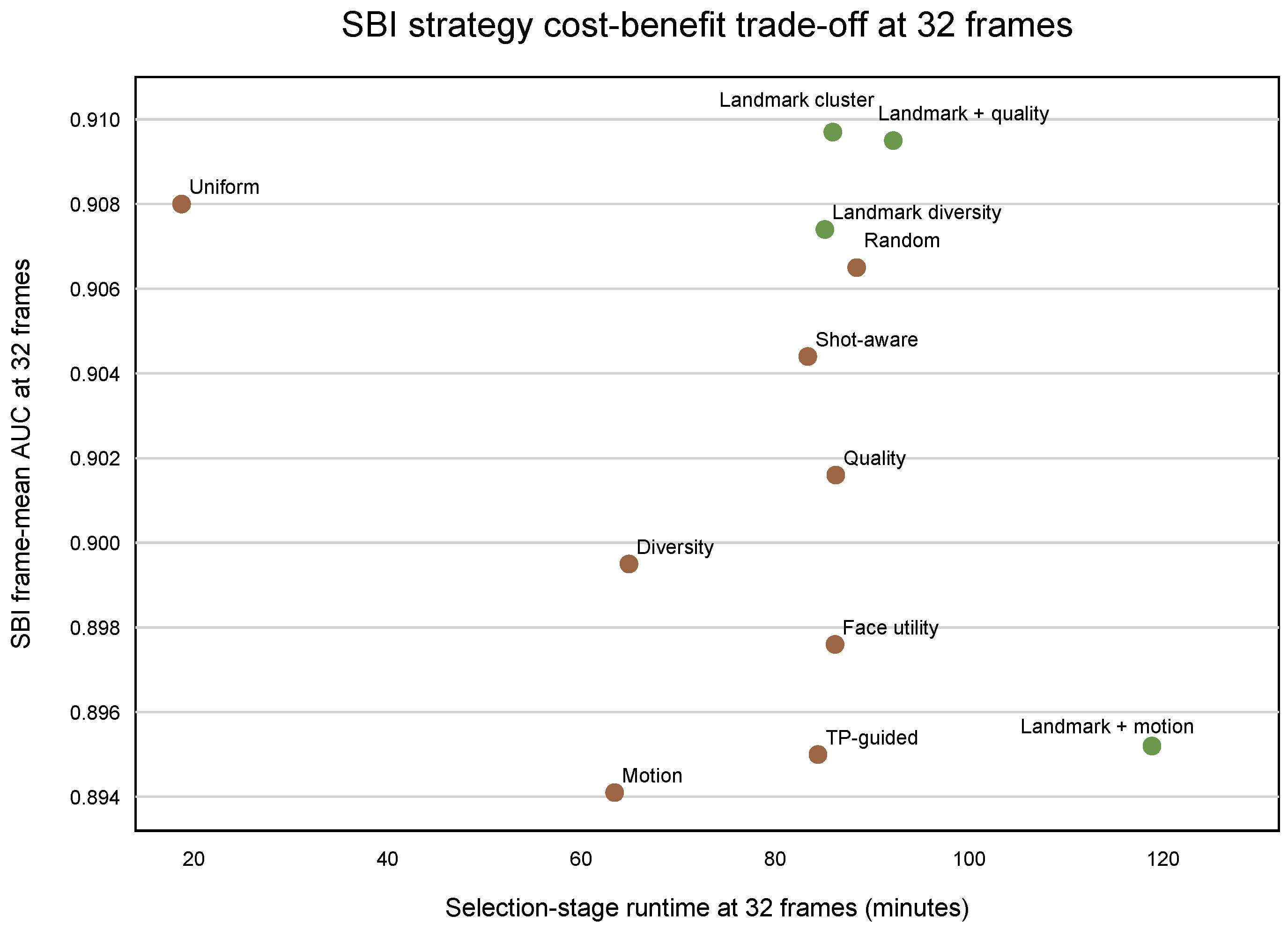
The heatmap is useful for understanding raw runtime growth, but the most useful view for decisions is the relation between cost and benefit at the largest tested budget. At 32 frames, Uniform remained by far the cheapest evaluated SBI selection policy at 18.7 min while still reaching a mean AUC of 0.9080. Landmark cluster achieved the strongest SBI result at the same budget, with an AUC of 0.9097, but required 86.0 min. Landmark + quality was nearly tied in accuracy at 0.9095 while taking 92.2 min. By contrast, Landmark + motion reached only 0.8952 AUC despite requiring 118.9 min, making it a particularly expensive configuration without a matching accuracy return.

This comparison clarifies that the completed benchmark does not reward complexity uniformly. Some expensive selection strategies improve accuracy slightly, but the gains can be marginal relative to their wall clock cost. In particular, the Pareto view in Figure 7 shows that Uniform remains a strong efficiency baseline, Landmark cluster is an accurate but much more expensive operating point, and Landmark + motion is dominated by cheaper alternatives with better or comparable performance. This type of cost analysis is important if frame selection is to be used in practical deployments rather than only as an offline benchmark variable.

The same observation can be summarized with a strict dominance criterion. At 32 frames, a strategy is considered dominated if another strategy achieves at least the same AUC at equal or lower runtime, with strict improvement in at least one of the two dimensions. Under this definition, ten of the twelve SBI strategies are dominated. Uniform dominates nine of them directly, while Landmark cluster dominates Landmark + quality by achieving slightly higher AUC at lower runtime. Consequently, only Uniform and Landmark cluster remain not dominated in the SBI comparison at 32 frames.

Table 7. Dominated SBI selection strategies at 32 frames.

Dominated Strategy	AUC	Runtime (min)	Dominated by	AUC	Runtime (min)
Diversity	0.8995	64.9	Uniform	0.9080	18.7
Quality	0.9016	86.3	Uniform	0.9080	18.7
Motion	0.8941	63.4	Uniform	0.9080	18.7
Shot-aware	0.9044	83.4	Uniform	0.9080	18.7
Face utility	0.8976	86.2	Uniform	0.9080	18.7
TP-guided	0.8950	84.4	Uniform	0.9080	18.7
Landmark diversity	0.9074	85.1	Uniform	0.9080	18.7
Landmark + quality	0.9095	92.2	Landmark cluster	0.9097	86.0
Landmark + motion	0.8952	118.9	Uniform	0.9080	18.7
Random	0.9065	88.4	Uniform	0.9080	18.7

lists the dominated configurations.

4.7. Detector Runtime Analysis Under Uniform Sampling

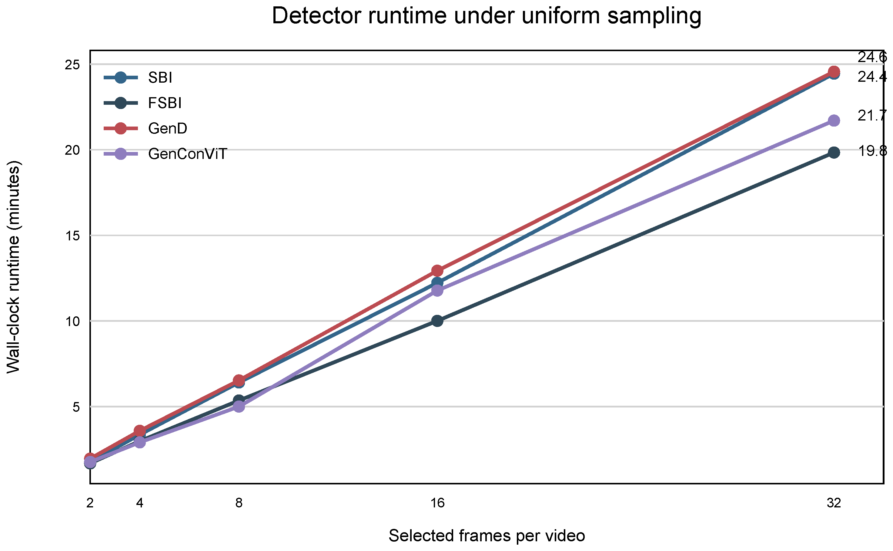
To complement the shared selection timings, a separate wall clock sweep after the benchmark was executed for the three external validated detectors under the Uniform strategy on the same manifest with 300 videos. This gives a simple runtime baseline at the detector level that is not confounded by the additional cost of more complex selection policies. Across all tested budgets, GenD was the slowest detector, while FSBI and GenConViT remained close to one another and exchanged the second place depending on the frame budget.

At 32 frames, the recorded wall clock times were 19.8 min for FSBI, 24.6 min for GenD, and 21.7 min for GenConViT. At 16 frames, the corresponding times were 10.0, 12.9, and 11.8 min. Thus, the strongest detector in accuracy terms, GenD, is also the most computationally expensive of the three measured external detectors under this common baseline. This result is useful for deployment interpretation because it shows that the detector with the highest AUC is not automatically the most efficient operating choice. Figure 8 shows the corresponding runtime curves under Uniform sampling.

4.8. Interpretation of Strategy Ranking

The average strategy ranking indicates that explicit geometric diversification is a strong principle for frame selection, but the completed benchmark also shows that landmark and heuristic strategies now form a tight top tier rather than two clearly separated groups. Landmark + quality and Landmark cluster remain among the best general purpose choices, yet Quality and Shot-aware are nearly tied with them. At the same time, the best strategy is not identical across models. Figure 9 summarizes these detector-specific best configurations. Therefore, the present results support two complementary conclusions: first, landmark strategies are strong general candidates for efficient deepfake detection; second, interactions between detector architecture and frame selection policy still matter and should be analyzed separately.

5. Discussion

The completed benchmark revises the strongest version of the original low budget hypothesis. In the complete factorial study with 300 videos, the best absolute average operating point is not 8 or 16 selected frames, but 32 selected frames. This is consistent across all four validated detectors. However, the more practically important observation is that the gains become small beyond the middle range of budgets. The average AUC rises from 0.8957 at 2 frames to 0.9189 at 8 frames, then only to 0.9218 at 16 frames and 0.9257 at 32 frames. The bootstrap confidence intervals of the higher budget means overlap substantially, which further supports a diminishing returns interpretation rather than a strong qualitative separation between 8, 16, and 32 frames. The expanded validation experiment with 1180 videos was added specifically to test this interpretation on a larger deduplicated sample. In that larger split, the complete grids for 2, 4, and 8 frames again show increasing mean AUC with increasing budget for all 4 detectors, while the reported subset at 16 frames remains compatible with a diminishing returns interpretation. Thus, 8 and especially 16 frames should be interpreted as efficient operating points that recover most of the attainable performance, not as settings that universally dominate the largest tested budget.

This distinction matters for the interpretation of novelty. The present manuscript does not claim that fewer frames universally outperform larger budgets. Instead, its contribution is a controlled and detector consistent quantification of the marginal returns of additional frames under a shared selection cache used during inference. By keeping the detector weights fixed and reusing the same selected inputs across SBI, FSBI, GenConViT, and GenD, the study isolates the effects of frame selection from the effects of retraining. This allows the benchmark to answer a more specific question than most prior detector papers, namely how much performance is gained by moving from 2 to 4, 8, 16, and 32 selected frames under the same downstream conditions.

The strategy ranking also became more nuanced in the completed benchmark. Selection based on landmarks remains strong, with Landmark + quality achieving the highest mean AUC and Landmark cluster remaining in the top tier. At the same time, the gap to the best heuristic strategies is small: Quality and Shot-aware are nearly tied with the best landmark strategy in the validated subset. The Pareto view with runtime makes this even clearer: some sophisticated policies improve accuracy only marginally relative to Uniform, while others such as Landmark + motion become expensive without competitive AUC. Therefore, the evidence supports geometric diversification as a robust general principle, but it does not support an overly strong claim that landmark methods dominate all alternatives under all conditions.

Interactions specific to each detector remain important. All 4 validated detectors achieve their best mean AUC at 32 selected frames, yet the preferred strategy differs by model: Landmark cluster for SBI, Uniform for FSBI, Diversity for GenConViT, and Shot-aware for GenD. This indicates that frame selection should not be treated as a universal preprocessing choice detached from detector architecture. Instead, it should be tuned jointly with the detector when inference cost, latency, or deployment constraints matter.

These findings complement earlier deepfake detection studies, which mainly focus on detector design and usually adopt a fixed frame count during inference [1,2,3]. In contrast, the present work shows that frame selection during inference is itself a meaningful experimental variable that changes the relation between cost and accuracy even when the detector is kept fixed. The shared selection cache is important in this context because it ensures that all detectors are compared on exactly the same selected inputs, and therefore makes differences between detectors easier to interpret.

The current conclusions should be interpreted within the scope of the benchmark. The complete factorial evidence is based on 300 videos drawn from Celeb-DF-v2, Celeb-DF++, and FaceForensics++, while the larger validation evidence uses a deduplicated split of 1180 Celeb-DF++ and FaceForensics++ videos with complete coverage at 2, 4, and 8 frames and a reported subset at 16 frames. The detector evidence is restricted to four validated pretrained models. The study also uses visual information only and does not address audio or multimodal cues. Future work should therefore extend the comparison to a larger detector set, test the same strategies on broader datasets and compression conditions, and report explicit runtime and energy savings in addition to classification metrics.

The study indicates that frame selection is not merely a technical detail to reduce the input size. It is a meaningful design choice that shapes the final decision for the video, and its practical value lies less in beating the largest frame budget than in showing how close smaller budgets can come to the same performance under controlled conditions.

6. Conclusions

This study demonstrates that frame selection is an important component of visual deepfake detection under constrained inference budgets. In the completed benchmark with 300 videos, 3 source datasets, and 4 validated detectors, the strongest average operating point is 32 selected frames. However, the benchmark also shows that most of the attainable performance is already recovered at 8 and 16 selected frames, and the bootstrap confidence intervals of the higher budget means overlap substantially. The expanded validation experiment with 1180 videos further supports the smaller budget interpretation on a substantially larger deduplicated sample: the complete grids at 2, 4, and 8 frames improve monotonically for all 4 detectors, and the reported subset at 16 frames remains consistent with the same diminishing returns pattern. Therefore, the practical question is not whether 32 frames are best in absolute terms but how much accuracy is sacrificed when substantially smaller budgets are used.

The benchmark also shows that detector ranking and frame selection ranking should be interpreted separately. At the detector level, GenD is the strongest validated model, achieving a mean AUC of 0.9464. At the strategy level, Landmark + quality is the strongest average selection method with a mean AUC of 0.9197, followed closely by Quality, Shot-aware, and Landmark cluster. However, the comparison with runtime shows that not every stronger or more complex strategy is cost effective: Uniform remains a strong efficiency baseline, whereas some expensive hybrids do not yield proportionally better accuracy. Therefore, the study captures not only differences in detector quality but also the independent contribution of the selection policy itself under a controlled shared cache protocol.

A further important conclusion is that strategies based on landmarks are strong general choices but do not eliminate behavior specific to each detector. The best configuration for GenD is Shot-aware sampling at 32 frames, while the other detectors prefer different strategies, even though all peak at the same budget. This supports continued investigation of geometric diversification after pose compensation, but it also advocates tuning with the detector in mind rather than using a universal frame selection policy.

The present manuscript should be interpreted as a reproducible benchmark of frame selection during inference rather than as a claim that low budgets universally outperform larger ones. Its main contribution is the controlled comparison itself: a shared prepared cache, 12 strategies, a complete reference at 32 frames in the factorial benchmark with 300 videos, and a larger validation with 1180 videos for the lower budget regimes. The same benchmark protocol can be extended directly with additional validated detectors and larger validation grids, making the current study a useful baseline for future comparative evaluation.

References

- Shiohara, K.; Yamasaki, T. Detecting deepfakes with self-blended images. In Proceedings of the IEEE/CVF Conference on Computer Vision and Pattern Recognition, New Orleans, LA, USA, 19–20 June 2022; pp. 18720–18729. [Google Scholar] [CrossRef]
- Deressa, D.W.; Mareen, H.; Lambert, P.; Atnafu, S.; Akhtar, Z.; Van Wallendael, G. GenConViT: Deepfake video detection using generative convolutional vision transformer. Appl. Sci. 2025, 15, 6622. [Google Scholar] [CrossRef]
- Yermakov, A.; Cech, J.; Matas, J.; Fritz, M. Deepfake detection that generalizes across benchmarks. In Proceedings of the IEEE/CVF Winter Conference on Applications of Computer Vision, Tucson, AZ, USA, 6–10 March 2026; pp. 773–783. [Google Scholar] [CrossRef]
- Yan, Z.; Zhang, Y.; Yuan, X.; Lyu, S.; Wu, B. Deepfakebench: A comprehensive benchmark of deepfake detection. arXiv 2023, arXiv:2307.01426. [Google Scholar] [CrossRef]
- Korshunov, P.; Marcel, S. DeepFakes: A New Threat to Face Recognition? Assessment and Detection. arXiv 2018, arXiv:1812.08685. [Google Scholar] [CrossRef]
- Afchar, D.; Nozick, V.; Yamagishi, J.; Echizen, I. MesoNet: A Compact Facial Video Forgery Detection Network. In Proceedings of the 2018 IEEE International Workshop on Information Forensics and Security (WIFS), Hong Kong, China, 11–13 December 2018; pp. 1–7. [Google Scholar] [CrossRef]
- Nguyen, H.H.; Yamagishi, J.; Echizen, I. Capsule-Forensics: Using Capsule Networks to Detect Forged Images and Videos. In Proceedings of the 2019 IEEE International Conference on Acoustics, Speech and Signal Processing (ICASSP), Brighton, UK, 12–17 May 2019; pp. 2307–2311. [Google Scholar] [CrossRef]
- Li, Y.; Lyu, S. Exposing DeepFake Videos By Detecting Face Warping Artifacts. In Proceedings of the IEEE/CVF Conference on Computer Vision and Pattern Recognition Workshops (CVPRW), Long Beach, CA, USA, 16–17 June 2019. [Google Scholar] [CrossRef]
- Rössler, A.; Cozzolino, D.; Verdoliva, L.; Riess, C.; Thies, J.; Nießner, M. FaceForensics++: Learning to Detect Manipulated Facial Images. In Proceedings of the IEEE/CVF International Conference on Computer Vision (ICCV), Seoul, Repubic of Korea, 27 October–2 November 2019; pp. 1–11. [Google Scholar] [CrossRef]
- Qian, Y.; Yin, G.; Sheng, L.; Chen, Z.; Shao, J. Thinking in Frequency: Face Forgery Detection by Mining Frequency-aware Clues. In Computer Vision—ECCV 2020; Springer: Berlin/Heidelberg, Germany, 2020; pp. 86–103. [Google Scholar] [CrossRef]
- Liu, H.; Li, X.; Zhou, W.; Chen, Y.; He, Y.; Xue, H.; Zhang, W.; Yu, N. Spatial-Phase Shallow Learning: Rethinking Face Forgery Detection in Frequency Domain. In Proceedings of the IEEE/CVF Conference on Computer Vision and Pattern Recognition (CVPR), Nashville, TN, USA, 19–25 June 2021; pp. 772–781. [Google Scholar] [CrossRef]
- Luo, Y.; Zhang, Y.; Yan, J.; Liu, W. Generalizing Face Forgery Detection With High-Frequency Features. In Proceedings of the IEEE/CVF Conference on Computer Vision and Pattern Recognition (CVPR), Nashville, TN, USA, 20–25 June 2021; pp. 16317–16326. [Google Scholar] [CrossRef]
- Wang, Y.; Yu, K.; Chen, C.; Hu, X.; Peng, S. Dynamic Graph Learning with Content-Guided Spatial-Frequency Relation Reasoning for Deepfake Detection. In Proceedings of the IEEE/CVF Conference on Computer Vision and Pattern Recognition (CVPR), Vancouver, BC, Canada, 17–24 June 2023; pp. 7278–7287. [Google Scholar] [CrossRef]
- Zhao, H.; Wei, T.; Zhou, W.; Zhang, W.; Chen, D.; Yu, N. Multi-attentional Deepfake Detection. In Proceedings of the 2021 IEEE/CVF Conference on Computer Vision and Pattern Recognition (CVPR), Nashville, TN, USA, 20–25 June 2021; IEEE: Piscataway, NJ, USA, 2021; pp. 2185–2194. [Google Scholar] [CrossRef]
- Zhao, T.; Xu, X.; Xu, M.; Ding, H.; Xiong, Y.; Xia, W. Learning Self-Consistency for Deepfake Detection. In Proceedings of the IEEE/CVF International Conference on Computer Vision (ICCV), Montreal, QC, Canada, 10–17 October 2021. [Google Scholar] [CrossRef]
- Chen, S.; Yao, T.; Chen, Y.; Ding, S.; Li, J.; Ji, R. Local Relation Learning for Face Forgery Detection. In Proceedings of the AAAI Conference on Artificial Intelligence, Virtual, 2–9 February 2021. [Google Scholar] [CrossRef]
- Fei, J.; Dai, Y.; Yu, P.; Shen, T.; Xia, Z.; Weng, J. Learning Second Order Local Anomaly for General Face Forgery Detection. In Proceedings of the IEEE/CVF Conference on Computer Vision and Pattern Recognition (CVPR), New Orleans, LA, USA, 19–20 June 2022. [Google Scholar] [CrossRef]
- Zhuang, W.; Chu, Q.; Tan, Z.; Liu, Q.; Yuan, H.; Miao, C.; Luo, Z.; Yu, N. UIA-ViT: Unsupervised inconsistency-aware method based on vision transformer for face forgery detection. In Proceedings of the European Conference on Computer Vision; Springer: Berlin/Heidelberg, Germany, 2022; pp. 391–407. [Google Scholar] [CrossRef]
- Huang, B.; Wang, Z.; Yang, J.; Ai, J.; Zou, Q.; Wang, Q.; Ye, D. Implicit Identity Driven Deepfake Face Swapping Detection. In Proceedings of the IEEE/CVF Conference on Computer Vision and Pattern Recognition (CVPR), Vancouver, BC, Canada, 17–24 June 2023. [Google Scholar] [CrossRef]
- Li, L.; Bao, J.; Zhang, T.; Yang, H.; Chen, D.; Wen, F.; Guo, B. Face X-ray for More General Face Forgery Detection. In Proceedings of the IEEE/CVF Conference on Computer Vision and Pattern Recognition (CVPR), Seattle, WA, USA, 13–19 June 2020. [Google Scholar] [CrossRef]
- Cao, J.; Ma, C.; Yao, T.; Chen, S.; Ding, S.; Yang, X. End-to-End Reconstruction-Classification Learning for Face Forgery Detection. In Proceedings of the IEEE/CVF Conference on Computer Vision and Pattern Recognition (CVPR), New Orleans, LA, USA, 19–20 June 2022; pp. 4113–4122. [Google Scholar] [CrossRef]
- Chen, L.; Zhang, Y.; Song, Y.; Liu, L.; Wang, J. Self-Supervised Learning of Adversarial Example: Towards Good Generalizations for Deepfake Detection. In Proceedings of the IEEE/CVF Conference on Computer Vision and Pattern Recognition (CVPR), New Orleans, LA, USA, 19–20 June 2022. [Google Scholar] [CrossRef]
- Cheng, J.; Yan, Z.; Zhang, Y.; Luo, Y.; Wang, Z.; Li, C. Can We Leave Deepfake Data Behind in Training Deepfake Detector? In Proceedings of the Advances in Neural Information Processing Systems, Vancouver, BC, Canada, 10–15 December 2024. [Google Scholar] [CrossRef]
- Li, H.; Zhou, J.; Li, Y.; Wu, B.; Li, B.; Dong, J. FreqBlender: Enhancing DeepFake Detection by Blending Frequency Knowledge. In Proceedings of the Advances in Neural Information Processing Systems, Vancouver, BC, Canada, 10–15 December 2024. [Google Scholar] [CrossRef]
- Wang, Z.; Bao, J.; Zhou, W.; Wang, W.; Li, H. AltFreezing for More General Video Face Forgery Detection. In Proceedings of the IEEE/CVF Conference on Computer Vision and Pattern Recognition (CVPR), Vancouver, BC, Canada, 17–24 June 2023; pp. 4129–4138. [Google Scholar] [CrossRef]
- Yan, Z.; Zhang, Y.; Fan, Y.; Wu, B. UCF: Uncovering Common Features for Generalizable Deepfake Detection. In Proceedings of the IEEE/CVF International Conference on Computer Vision (ICCV), Paris, France, 1–6 October 2023. [Google Scholar] [CrossRef]
- Larue, N.; Vu, N.S.; Struc, V.; Peer, P.; Christophides, V. SeeABLE: Soft Discrepancies and Bounded Contrastive Learning for Exposing Deepfakes. In Proceedings of the IEEE/CVF International Conference on Computer Vision (ICCV), Paris, France, 1–6 October 2023. [Google Scholar] [CrossRef]
- Dong, S.; Wang, J.; Ji, R.; Liang, J.; Fan, H.; Ge, Z. Implicit Identity Leakage: The Stumbling Block to Improving Deepfake Detection Generalization. In Proceedings of the IEEE/CVF Conference on Computer Vision and Pattern Recognition (CVPR), Vancouver, BC, Canada, 17–24 June 2023. [Google Scholar] [CrossRef]
- Yan, Z.; Luo, Y.; Lyu, S.; Liu, Q.; Wu, B. Transcending Forgery Specificity with Latent Space Augmentation for Generalizable Deepfake Detection. In Proceedings of the IEEE/CVF Conference on Computer Vision and Pattern Recognition (CVPR), Seattle, WA, USA, 16–22 June 2024. [Google Scholar] [CrossRef]
- Choi, J.; Kim, T.; Jeong, Y.; Baek, S.; Choi, J. Exploiting Style Latent Flows for Generalizing Deepfake Video Detection. In Proceedings of the IEEE/CVF Conference on Computer Vision and Pattern Recognition (CVPR), Seattle, WA, USA, 16–22 June 2024; pp. 1133–1143. [Google Scholar] [CrossRef]
- Cui, X.; Li, Y.; Luo, A.; Zhou, J.; Dong, J. Forensics Adapter: Adapting CLIP for Generalizable Face Forgery Detection. In Proceedings of the IEEE/CVF Conference on Computer Vision and Pattern Recognition (CVPR), Nashville, TN, USA, 11–15 June 2025. [Google Scholar] [CrossRef]
- Yan, Z.; Yao, T.; Chen, S.; Zhao, Y.; Fu, X.; Zhu, J.; Luo, D.; Wang, C.; Ding, S.; Wu, Y.; et al. Df40: Toward next-generation deepfake detection. Adv. Neural Inf. Process. Syst. 2024, 37, 29387–29434. [Google Scholar] [CrossRef]
- Dincer, S.; Ulutas, G.; Ustubioglu, B.; Tahaoglu, G.; Sklavos, N. Golden Ratio Based Deep Fake Video Detection System with Fusion of Capsule Networks. Comput. Electr. Eng. 2024, 117, 109234. [Google Scholar] [CrossRef]
- Hu, J.; Liang, J.; Qin, Z.; Liao, X.; Zhou, W.; Lin, X. ADA-FInfer: Inferring Face Representations From Adaptive Select Frames for High-Visual-Quality Deepfake Detection. IEEE Trans. Dependable Secur. Comput. 2025, 22, 3011–3027. [Google Scholar] [CrossRef]
- Li, Y.; Yang, X.; Sun, P.; Qi, H.; Lyu, S. Celeb-df: A large-scale challenging dataset for deepfake forensics. In Proceedings of the IEEE/CVF Conference on Computer Vision and Pattern Recognition, Seattle, WA, USA, 13–19 June 2020; pp. 3207–3216. [Google Scholar] [CrossRef]
- Li, Y.; Zhu, D.; Cui, X.; Lyu, S. Celeb-DF++: A Large-scale Challenging Video DeepFake Benchmark for Generalizable Forensics. arXiv 2025, arXiv:2507.18015. [Google Scholar] [CrossRef]
Figure 1.
Illustrative frame selection examples for a real video. The numbers in the panels indicate selected-frame order. (a) Uniform, 4f. (b) Uniform, 8f. (c) Uniform, 16f. (d) Quality, 4f. (e) Quality, 8f. (f) Quality, 16f. (g) Landmark cluster, 4f. (h) Landmark cluster, 8f. (i) Landmark cluster, 16f. (j) Landmark + quality, 4f. (k) Landmark + quality, 8f. (l) Landmark + quality, 16f.
Figure 2.
Illustrative frame selection examples for a fake video. The numbers in the panels indicate selected-frame order. (a) Uniform, 4f. (b) Uniform, 8f. (c) Uniform, 16f. (d) Quality, 4f. (e) Quality, 8f. (f) Quality, 16f. (g) Landmark cluster, 4f. (h) Landmark cluster, 8f. (i) Landmark cluster, 16f. (j) Landmark + quality, 4f. (k) Landmark + quality, 8f. (l) Landmark + quality, 16f.
Figure 3.
Strategy ranking by mean AUC across frame selection strategies.
Figure 4.
Mean AUC by detector and frame budget.
Figure 5.
Bootstrap confidence intervals and AUC loss relative to 32 frames.
Figure 6.
SBI selection runtime by strategy and frame budget.
Figure 7.
SBI selection cost and accuracy at 32 frames.
Figure 8.
Detector runtime under Uniform sampling.
Figure 9.
Best validated configuration by detector.