RIS-Aided Path Loss Model Evaluation in Real-Life Scenarios

Abstract

One of the most intensively developed areas of wireless telecommunications in recent years is the practical application of reconfigurable intelligent surfaces (RISs). This paper presents the results of experimental research conducted at 5.5 GHz using a 16 × 16 element RIS to verify the accuracy of the Tang, Zheng, and Jeong theoretical models, which describe signal behavior upon reflection from an RIS. In contrast to purely simulation-based papers, this study utilizes different antenna types in a laboratory environment representative of a typical office space. The performance of the models is evaluated across distances of 1 m, 1.5 m, and 2 m through a comprehensive quantitative analysis. The study reports core error metrics, including mean and median root mean square error (RMSE), mean absolute error (MAE), and sum of squared differences (SSD), as well as the Interquartile Range (IQR) to assess modeling stability. Furthermore, a Wilcoxon signed-rank test is employed to statistically compare the modeling accuracy.

1. Introduction

Reconfigurable intelligent surfaces (RISs) represent one of the most rapidly evolving areas of wireless telecommunications [1,2]. Their popularity stems from an innovative approach to wireless system design, which allows for dynamic manipulation of the propagation environment by altering how signals are reflected by RIS. The core functionality of RIS is rooted in the use of metamaterials [3]—engineered surfaces composed of sub-wavelength structures that enable electromagnetic responses beyond the capabilities of naturally occurring substances. The transition from three-dimensional metamaterials to two-dimensional (2D) metasurface architectures triggers specific interface effects, allowing for the precise manipulation of electromagnetic fields through rapid phase and amplitude discontinuities [4,5]. In its basic form, RIS is a passive device composed of numerous antenna elements, each individually controlled to achieve a desired reflection characteristic. This is accomplished by precisely adjusting the amplitude and phase of the reflected electromagnetic waves [6,7].

Various RIS implementations with differing levels of control resolution have been described in the literature [8,9]. One of the key challenges in this field is the accurate theoretical modeling of RIS behavior, as the RIS-assisted channel is a cascade of three subchannels where the large-scale path loss is heavily dictated by the surface’s unique electromagnetic properties.

Early conceptual frameworks, such as the one by Basar et al. [10], illustrated the RIS mechanism by revisiting the two-ray path loss model, while Björnson and Sanguinetti [11] clarified power scaling laws by comparing RIS to massive Multiple-Input Multiple-Output (MIMO), proving that thousands of elements are required to compensate for the lack of active amplification. In parallel, Özdogan et al. [12] and Di Renzo et al. [13] utilized physical optics and the Huygens–Fresnel principle to define the conditions under which an RIS acts as an anomalous mirror rather than a simple scatterer.

Building upon this growing theoretical consensus, the works by Tang et al. [14,15] provided a pivotal benchmark for the community by introducing a comprehensive and experimentally validated path loss model. Their framework explicitly links received power to Tx/Rx antenna gains, the physical size and number of elements, and specific radiation patterns across three distinct scenarios: far-field beamforming, near-field beamforming, and near-field broadcasting. While Tang’s model is highly influential, it relies on certain simplifications, such as assuming a constant and identical reflection amplitude for all elements. Furthermore, its initial validation was performed under ideal anechoic conditions.

Consequently, more recent studies have focused on evaluating and extending these formulations for diverse environments and higher frequency bands. For instance, Kashif et al. [16] adapted these modeling principles to analyze performance in millimeter-wave and sub-THz bands, where precise beamforming gains become critical. These efforts are complemented by the practical investigations of Zheng et al. [17] and Jeong et al. [18], who evaluated the performance of these link-budget predictions in realistic, non-ideal environments, as we discuss later in the paper.

This work presents an evaluation of the true accuracy of selected theoretical models ([14,17,18]) in estimating received signal power when RIS is used in office environment. It is particularly important to emphasize that the measurement results are highly impacted (or might be highly impacted) when the surrounding environment changes. The selected experimentation scenario is the typical office with the number of computers, tables and chairs; however, change of the furniture deployment as well as modification of the elements present in the office will directly impact the multipath propagation between the transmitter and receiver. Knowing that, the results presented in the paper should be treated as the assessment of the selected three popular theoretical RIS models in the typical office environment. For the experiment, we apply the RIS presented in [9], which operates around 5.5 GHz; the drawn conclusions are then associated with this frequency band. The purpose of the study is to assess how accurately the proposed models reflect the actual propagation of the signal and whether further refinement is necessary to improve the accuracy of the prediction. The main contributions of the paper are the following:

• Direct evaluation of three widely accepted theoretical RIS models in the same experimentation scenario and their qualitative and statistical comparison using several metrics;
• Practical exemplification of the theoretical RIS model with one of the popular RIS boards;
• Comparison of the results for various patterns and three different distances.

The conducted experiments deliver a solid foundation for the assessment of the accuracy of theoretical models when they are applied in practical scenarios.

2. Theoretical Models

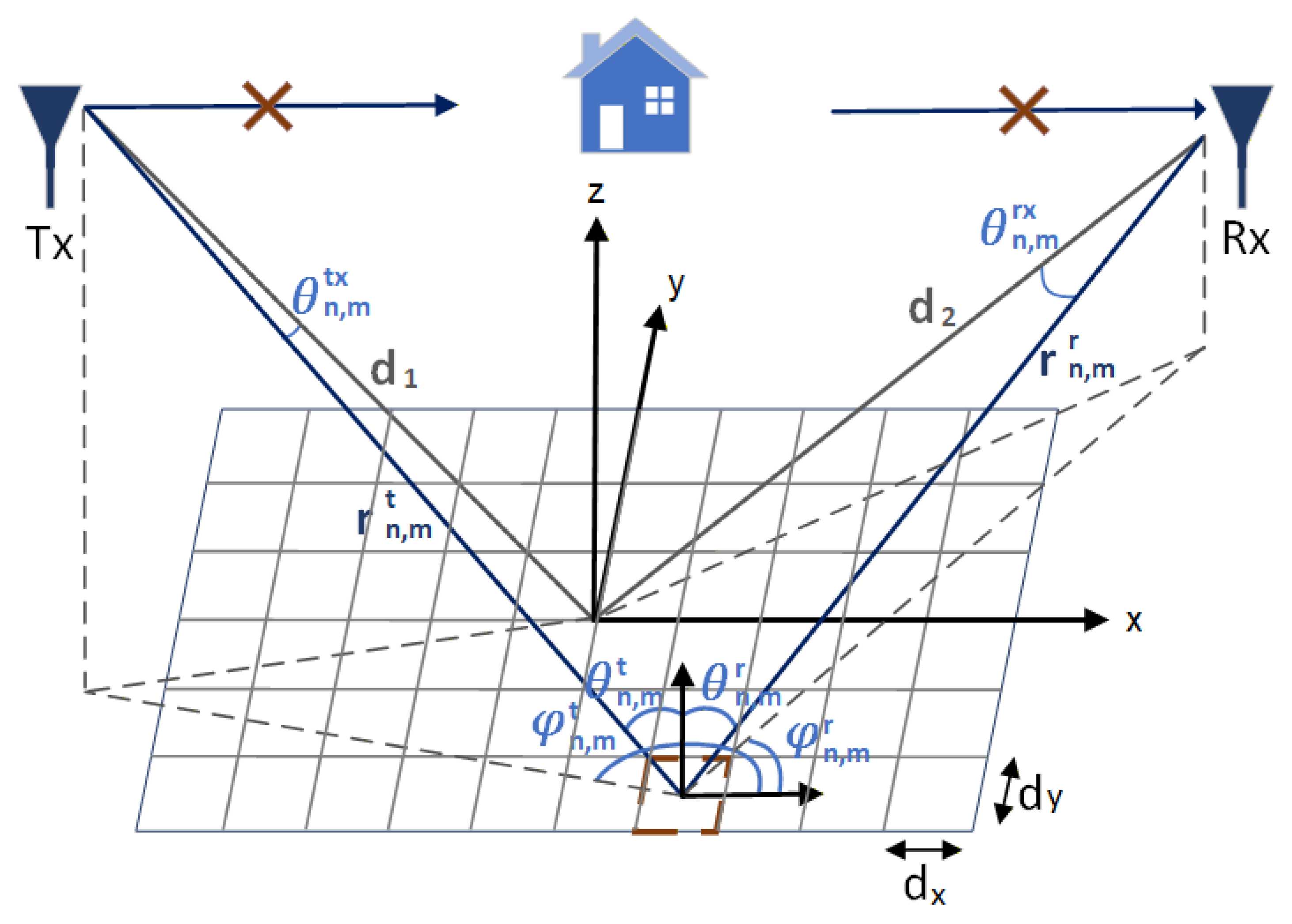
The estimation of the received power was performed using three distinct propagation models proposed by Tang, Zheng, and Jeong, which are compared in this article against each other and against measurement data [14,17,18]. In the considered scenario, wireless communication between the transmitter and receiver is supported by RIS due to the lack of a direct signal path between them, as illustrated in Figure 1. A global Cartesian coordinate system $(x,y,z)$ is defined, where the x- and y-axes lie in the plane of the RIS and the z-axis is perpendicular to its surface. The RIS is composed of discrete unit cells, with $U_{n,m}$ denoting the unit cell located in the n-th row and m-th column, and $d_x$ and $d_y$ representing the inter-element spacing along the x- and y-directions, respectively. The distance between the transmitter and the $(n,m)$-th RIS element is denoted by $r_{n,m}^t$, while $r_{n,m}^r$ denotes the distance between the $(n,m)$-th RIS element and the receiver. Parameters $d_1$ and $d_2$ describe distances from the transmitter to the center of RIS and from the center of RIS to the receiver, respectively. The angles ${\theta }_{n,m}^{\mathrm{tx}}$ and ${\theta }_{n,m}^{\mathrm{rx}}$ represent the elevation angles, and ${\phi }_{n,m}^{\mathrm{tx}}$ and ${\phi }_{n,m}^{\mathrm{rx}}$ denote the azimuth angles from the corresponding unit cell to the transmitter and receiver, respectively. In contrast ${\theta }_{n,m}^{\mathrm{t}}$ and ${\theta }_{n,m}^{\mathrm{r}}$ represent the elevation angles, and ${\phi }_{n,m}^{\mathrm{t}}$ and ${\phi }_{n,m}^{\mathrm{r}}$ represent the azimuth angles from the transmitter/receiver to the unit cell.

The analytical expressions for the received signal power employed in this analysis are derived for a scenario in which the receiver is located in the near field of the RIS. The near-field boundary can be determined using the following formula:

$$L_g={\displaystyle \frac{2D^2}{\lambda }}$$

(1)

where D is the largest physical dimension of RIS and $\lambda$ is the wavelength. For the RIS considered in the measurements and for the employed signal frequency, the near-field boundary is obtained as follows:

$$R_{ff}={\displaystyle \frac{2\times {\left(38.17\mathrm{cm}\right)}^2}{5.45\mathrm{cm}}}=5.35\mathrm{m}$$

(2)

To adopt realistic parameters for the theoretical models, we follow the information provided by the designers of these boards available in [19]. In particular, based on the magnitude impulse response, we have assumed that for operating frequency 5.5 GHz the magnitude for ON state is equal to −2 dB (or ${10}^{-2/20}=0.8$ in linear scale) and for OFF state −5.5 dB (or ${10}^{-5.5/20}=0.5$ in linear scale).

2.1. Tang’s Model

Tang et al. [14] proposed a detailed model for RIS-assisted wireless systems, in which the received signal power is computed as the coherent sum of contributions from all individual RIS elements, as shown in Equation (3). Each element reflects the incident wave with a controlled phase shift ${\varphi }_{n,m}$ and a radiation factor $F_{n,m}^{\mathrm{C}}$. In this model, a uniform reflection amplitude A is assumed for all elements, acting as a global scaling factor outside the summation. Furthermore, to ensure accuracy in the near-field region, the model precisely calculates the true local geometric angles and distances for each individual array element rather than employing a single central approximation angle.

$$\begin{array}{cc}\hfill & P_r=P_t{\displaystyle \frac{G_t{G}_{r}G{d}_x{d}_y{\lambda }^2{A}^2}{64{\pi }^3}}{\left|{\displaystyle \sum _{m=1-\frac{M}{2}}^{\frac{M}{2}}}{\displaystyle \sum _{n=1-\frac{N}{2}}^{\frac{N}{2}}}\sqrt{F_{n,m}^{\mathrm{C}}}{\displaystyle \frac{e^{\frac{-j(2\pi (r_{n,m}^t+r_{n,m}^r)-\lambda {\varphi }_{n,m})}{\lambda }}}{r_{n,m}^t{r}_{n,m}^r}}\right|}^2,\hfill \end{array}$$

(3)

where $P_t$ denotes the transmitted signal power, $G_t$ and $G_r$ are the gains of the transmitting and receiving antennas, respectively, while G represents the gain of a single antenna element of the RIS module. The symbol $\lambda$ refers to the wavelength, while A denotes the amplitude of the signal for each antenna element. The variable ${\varphi }_{n,m}$ represents the phase shift introduced by the RIS element with index $(n,m)$. For the binary RIS used in the measurements, ${\varphi }_{n,m}\in \{0,\pi \}$ radians. $F_{n,m}^{\mathrm{C}}$ is the cumulative radiation characteristic that takes into account the normalized radiation characteristics of the transmitter ($F^{tx}$), receiver ($F^{rx}$) and antenna element (F) according to the formula:

$$\begin{array}{cc}\hfill F_{n,m}^{\mathrm{C}}=& F^{\mathrm{tx}}\left({\theta }_{n,m}^{\mathrm{tx}},{\phi }_{n,m}^{\mathrm{tx}}\right)F\left({\theta }_{n,m}^t,{\phi }_{n,m}^t\right)F\left({\theta }_{n,m}^r,{\phi }_{n,m}^r\right)F^{\mathrm{rx}}\left({\theta }_{n,m}^{\mathrm{rx}},{\phi }_{n,m}^{\mathrm{rx}}\right).\hfill \end{array}$$

(4)

The specific normalized power radiation pattern $F\left(\theta ,\phi \right)$ is only a function of elevation angle $\theta$ and is maximized when $\theta =0$:

$$F(\theta ,\varphi )=\left\{\begin{array}{cc}{cos}^3\theta ,\hfill & 0\le \theta \le {\displaystyle \frac{\pi }{2}}\hfill \\ 0,\hfill & {\displaystyle \frac{\pi }{2}}<\theta \le \pi .\hfill \end{array}\right.$$

(5)

Table 1. Key parameter values used in Tang’s formula.

RIS Size	${\mathit{P}}_{\mathit{t}}$ [dBm]	A	dx [mm]	dy [mm]	$\mathit{\lambda }$ [cm]	G [dBi]
$16\times 16$	−10	0.65	20	13	5.45	1

presents the key parameter values substituted into the formula of the Tang’s model. Note that for this model, a single amplitude value $A=0.65$ was applied uniformly to all elements regardless of their phase state, representing the arithmetic mean of the ON ($0.8$) and OFF ($0.5$) state amplitudes derived from the hardware specifications [19].

2.2. Zheng’s Model

Zheng et al. [17] proposed a model for discrete-phase-shift RIS based on the Friis transmission equation and fundamental electromagnetic principles. In this approach, the binary phase shifts are similarly mapped as ${\varphi }_{n,m}\in \{0,\pi \}$. However, this model explicitly accounts for state-dependent amplitude losses by keeping the amplitude parameter $A_{n,m}$ inside the summation. Similarly to the Tang model, the geometric distances and local angles are calculated individually for each unit cell to maintain accuracy in the near-field zone. The received signal power is calculated as follows:

$$\begin{array}{cc}\hfill & P_r=P_t{\displaystyle \frac{G_t{G}_{r}G{d}_x{d}_y{\lambda }^2}{64{\pi }^3}}{\left|{\displaystyle \sum _{m=1-\frac{M}{2}}^{\frac{M}{2}}}{\displaystyle \sum _{n=1-\frac{N}{2}}^{\frac{N}{2}}}\sqrt{F_{n,m}^{\mathrm{C}}}{A}_{n,m}{\displaystyle \frac{e^{\frac{-j(2\pi (r_{n,m}^t+r_{n,m}^r)-\lambda {\varphi }_{n,m})}{\lambda }}}{r_{n,m}^t{r}_{n,m}^r}}\right|}^2.\hfill \end{array}$$

(6)

The amplitude $A_{n,m}$ is assigned per-element based on its phase state: $A_{n,m}=A_{ON}=0.8$ for ${\varphi }_{n,m}=\pi$, and $A_{n,m}=A_{OFF}=0.5$ for ${\varphi }_{n,m}=0$. These discrete values were substituted for each element $(n,m)$ individually, rather than using a global average.

Table 2. Key parameter values used in Zheng’s formula.

RIS Size	${\mathit{P}}_{\mathit{t}}$ [dBm]	${\mathit{A}}_{\mathit{ON}}$	${\mathit{A}}_{\mathit{OFF}}$	dx [mm]	dy [mm]	$\mathit{\lambda }$ [cm]	G [dBi]
$16\times 16$	−10	0.8	0.5	20	13	5.45	1

lists the key parameter values used in the Zheng model formula.

2.3. Jeong’s Model

Jeong et al. [18] proposed a path loss model that considers practical electromagnetic phenomena such as unit cell phase errors and specular reflection loss. In contrast to the Tang and Zheng models, which employ element-wise calculations, this model utilizes a simplified “central approximation” for the geometry, assuming uniform angles and distances for the entire RIS surface. The received power obtained from analyses of the practical RIS-aided environment was derived and is given by

$$\begin{array}{cc}\hfill & P_r=P_t{K}^2{L}_{PE}{L}_{SR}{\left({\displaystyle \frac{S_p}{4\pi }}\right)}^2{\displaystyle \frac{cos{\theta }_{ic}cos{\theta }_{rc}{G}_t{G}_r}{d_1^2{d}_2^2}}{\left|{\Gamma }_{av}\right|}^2,\hfill \end{array}$$

(7)

where $K=N\times M$ is the number of RIS elements, $L_{PE}$ and $L_{SR}$ are the phase error and specular reflection loss of the RIS, respectively, $S_p$ is the area of a single RIS element, ${\theta }_{ic}$ and ${\theta }_{rc}$ denote the angles of incidence and reflection at the RIS center, $G_t$ and $G_r$ are the transmitter and receiver antenna gains, and $d_1$ and $d_2$ are the distances from the transmitter to the RIS and from the RIS to the receiver, respectively. ${\Gamma }_{av}$ represents the average reflection amplitude of all unit cells, considering that the reflection amplitude is equal to 0.5 when a unit cell is in the OFF state and 0.8 when it is in the ON state.

Table 3. Key parameter values used in Jeong’s formula.

RIS Size	${\mathit{P}}_{\mathit{t}}$ [dBm]	${\mathit{A}}_{\mathit{ON}}$	${\mathit{A}}_{\mathit{OFF}}$	${\mathit{L}}_{\mathit{PE}}$ [dB]	${\mathit{L}}_{\mathit{SR}}$ [dB]	dx [mm]	dy [mm]	$\mathit{\lambda }$ [cm]
$16\times 16$	−10	0.8	0.5	0	0	20	13	5.45

provides the key parameter values substituted into the Jeong model equation.

3. Measurement Environments

The measurement campaign was designed to investigate the reflection characteristics of reconfigurable intelligent surfaces under different propagation conditions and with different antenna types. For this purpose, a dedicated measurement setup was developed and used in all considered cases. The setup consisted of three main functional blocks: signal generation, signal reception and analysis, and RIS control. All components were interconnected through a commercial router and operated remotely by a control computer running dedicated software. The parameters of spectrum analyzer are presented in

Table 4. Parameters of spectrum analyzer.

Parameter	Value	Unit
Frequency span	0	Hz
RBW	500	Hz
Sweep time	50	ms
Reference level	−30	dBm
Center frequency	5.5	GHz
Noise level	−110	dBm
Operating mode	Max Hold

.

Measurements were conducted for three different configurations, varying in both the propagation environment and the antennas used. The first set of measurements, hereafter referred to as Scenario 1, was performed in an office environment using Ainfo directional antennas (antenna parameters are provided in

Table 5. Parameters of the antennas used.

Antenna	Model	Frequency [GHz]	Gain [dBi]	3 dB Angle E/H [°]
METIS	14HV	5.1–5.9	14	32/35
AINFO	LB-187-20-C-SF	3.95–5.85	20	16/18

). The room contained desks and chairs placed along two side walls, with monitors, computers, and typical office equipment located on the desks, which acted as additional scattering objects. The measurement setup was positioned near one end of the room to reduce the influence of reflections from the opposite wall. The second set, referred to as Scenario 2, was likewise conducted in an office environment, utilizing Metis microstrip antennas. A detailed description of this scenario can be found in [20,21]. The third set of measurements, referred to as Scenario 3, took place under ideal conditions in an anechoic chamber and also employed Metis antennas. These environments were selected to capture both realistic indoor propagation conditions, represented by the office scenarios with two different antenna types, and an idealized reference case provided by the anechoic chamber, enabling evaluation of the considered RIS model accuracy in practical settings and comparison with controlled, interference-free measurements.

In all scenarios, the transmitting part of the setup was based on a Rohde & Schwarz SMM100A signal generator. A continuous-wave signal at 5.5 GHz with an output power of $-10$ dBm was transmitted toward the RIS. The reflected signal was received by the corresponding antenna and measured using a Rohde & Schwarz FSV3000 spectrum analyzer (Rohde & Schwarz, Munich, Germany) operating in Max Hold mode. Both transmitting and receiving antennas were vertically polarized and carefully aligned toward the center of the RIS surface to ensure repeatable measurement conditions. The antennas and matrix were placed at the height of H = 1.3 m.

For these experiments, an RIS module based on the open-source design introduced in [9] was used, enabling flexible control and customization of the RIS elements operating in the 5 GHz band. The employed RIS board consisted of 256 elements arranged in a $16\times 16$ array, with each element controlled by a single bit. This allowed binary phase control, where the reflected signal experienced either no phase shift in OFF state or a ${180}^{\circ }$ phase shift in ON state. Despite the simplicity of this control mechanism, the number of possible RIS states remained extremely large, resulting in a broad operational space.

The RIS was controlled by a dedicated single-board computer running a custom Python script responsible for synchronizing all measurement components. The same control framework was also used to remotely configure the signal generator, the spectrum analyzer, and the RIS phase states. Although the full configuration space of the RIS is very large, 27 phase patterns were selected for measurement and analysis. These patterns included both regular structures proposed in earlier studies and additional pseudo-random configurations introduced for comparative purposes.

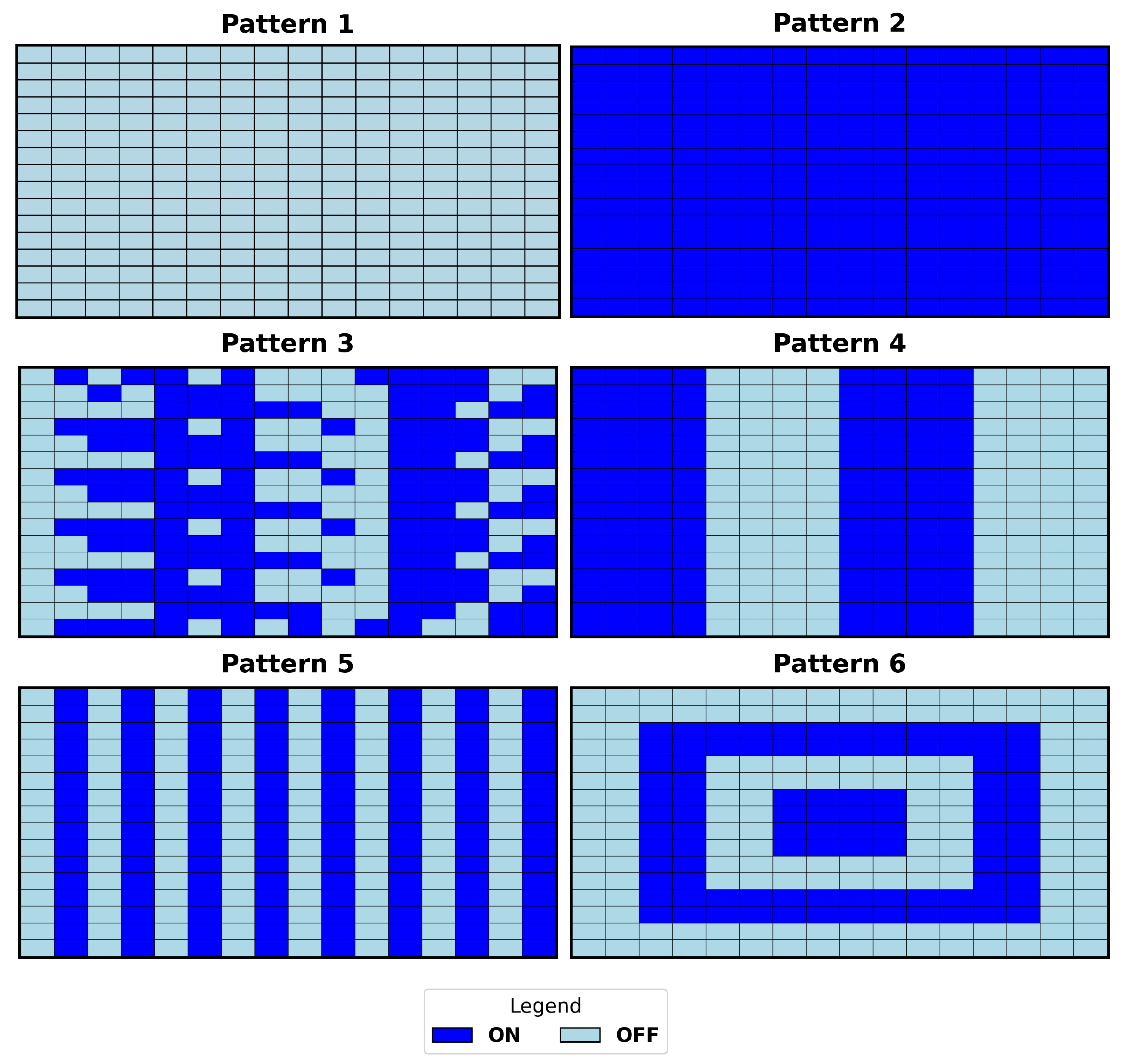
In each scenario, to analyze the directional reflection characteristics, the RIS was rotated only in the azimuth plane over angles ranging from $\phi ={45}^{\circ }$ to ${135}^{\circ }$, with an angular resolution of $1.8^{\circ }$. Measurements were performed for 27 RIS phase patterns; however, this article presents the results for the six most representative configurations, illustrated in Figure 2, where each pattern represents the full RIS matrix and explicitly shows the state of each individual element (dark cells corresponding to ON elements and light cells to OFF elements).

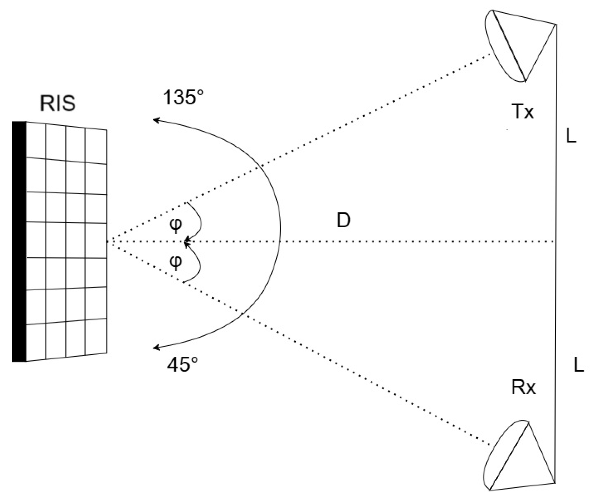
The measurement geometry was examined for three different distances between the antenna line and the RIS board, namely D = 1 m, 1.5 m, and 2 m. In all cases, the spacing between the transmitting and receiving antennas remained constant at 2L = 2 m, which resulted in antenna orientation angles toward the RIS equal to $45.0^{\circ }$, $56.3^{\circ }$, and $63.4^{\circ }$, respectively (Figure 3). For the operating frequency of 5.5 GHz, the wavelength was equal to $\lambda =0.0545$ m. Consequently, the beginning of the far-field region could be estimated from the Fraunhofer criterion as

$$R_{\mathrm{FF}}\ge {\displaystyle \frac{2D^2}{\lambda }}.$$

4. Results and Discussion

Comparing the obtained results with those predicted by theoretical models enables a comprehensive analysis of the influence of both the measurement environment and antenna parameters on the overall characteristics of the RIS module. This comparison facilitates the validation of the models and the identification of potential deviations arising from practical factors, such as interference, imperfections of the RIS elements, or system nonlinearities.

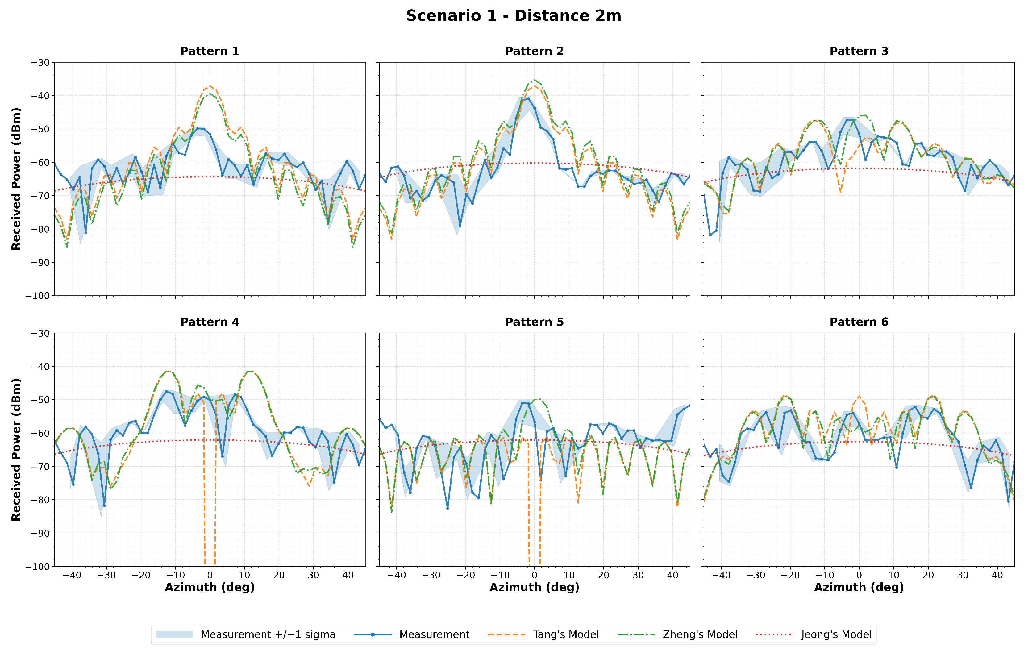
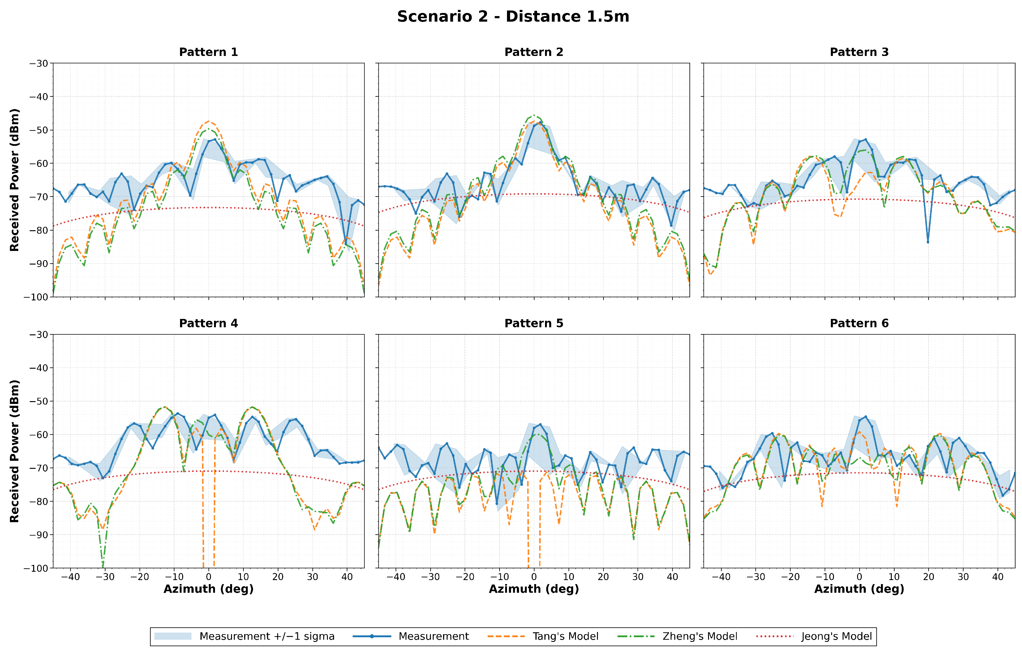
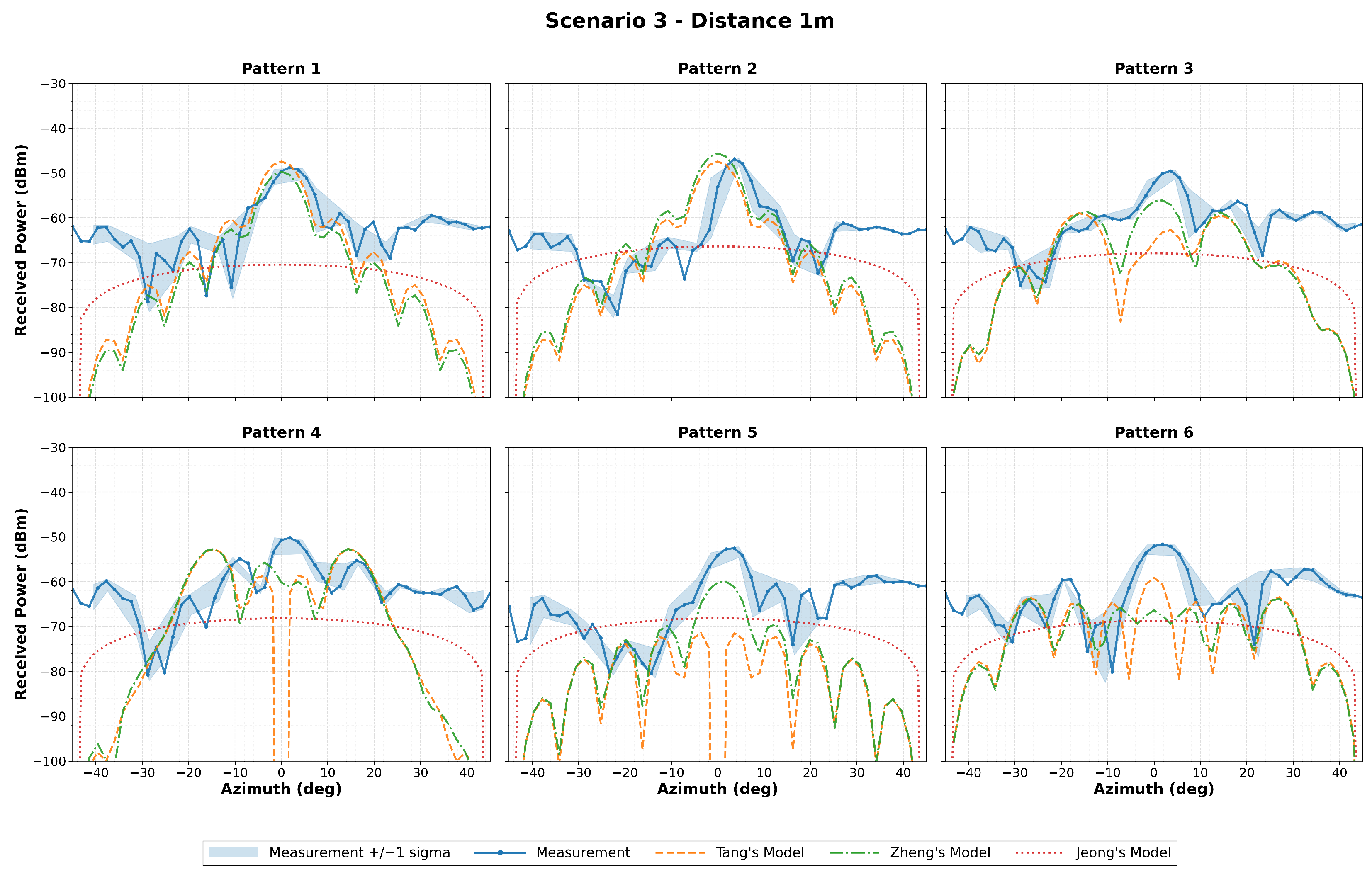
Figure 4, Figure 5 and Figure 6 present a comparison between the measured received power and the values predicted by three theoretical models for different RIS patterns and three RIS–antenna distances of 1 m, 1.5 m, and 2 m, respectively. Each figure includes results for six representative RIS patterns. The blue curve represents the measured data, while the orange, green, and red curves correspond to Tang’s model, Zheng’s model, and Jeong’s model, respectively. The shaded blue region indicates the measurement uncertainty, expressed as the standard deviation calculated from measurements taken at ±3° around each angular position.

In Figure 4, the measured characteristics show pronounced angular selectivity with visible local fades and secondary peaks. Tang’s model and Zheng’s model usually follow the shape of the measured curves more closely, capturing the main lobe direction and several secondary oscillations, although they often exaggerate the dynamic range and produce deeper nulls than observed in measurements (e.g., Patterns 4 and 5, where sharp notches appear for 0°). This effect results directly from the array pattern itself—for these RIS configurations the phase distribution leads to a near-cancellation of the complex field contributions, driving the coherent sum in (3) close to zero. This indicates that the ideal coherent summation assumed in the model is more sensitive to phase cancellation than the real measurement setup, leading to sharper simulated minima. In practice, measurement imperfections, mutual coupling, amplitude/phase errors and scattering prevent such perfect cancellation, hence the measured nulls are shallower than those predicted by the model. Model 3 produces much smoother, quasi-parabolic characteristics with weak angular variation; since this model does not incorporate pattern-dependent RIS reconfiguration, its response should be interpreted as a baseline angular trend rather than a pattern-specific prediction. The best qualitative agreement is observed for Pattern 2 and Pattern 3, where both Tang’s model and Zheng’s model correctly track the main lobe and its width.

For Figure 5, the overall behavior remains similar, but the measured curves are slightly smoother and the angular power spread is reduced compared to the 1 m case in the first scenario. The consistency between measurements and Tang’s model, and Zheng’s model improves for several patterns, particularly Pattern 2 and Pattern 6, where the main lobe level and its angular span are well reproduced. However, systematic level offsets are still visible in some angular regions, and deep modeled nulls are not always confirmed by measurements. Jeong’s model shows good agreement with the measurements in terms of the global angular trend and average power level, providing a smooth envelope that follows the azimuth dependence, although it does not reproduce local fades and secondary lobes visible in the measured characteristics.

In Figure 6, the agreement between measurements and the more detailed models (Tang’s model, Zheng’s model) is in many cases the best among all tested distances. The measured patterns become more regular and the main lobes are more clearly defined, which is well captured especially by Zheng’s model (green curves). Patterns 1 and 2 again shows the closest match in both lobe direction and peak level. Some discrepancies remain in the side-lobe structure and notch depths (notably for Patterns 4 and 5), where the models predict sharper fades than those measured. At this distance, Jeong’s model remains well aligned with the measured average level over a wide azimuth range and can be treated as a stable reference background, against which the angular selectivity predicted by the more detailed models can be compared.

Across all three scenarios, the results indicate that the more detailed models (Tang’s model, Zheng’s model) correctly predict the main beam direction for all analyzed patterns and distances, but exhibit an azimuth-dependent level bias and tend to overestimate angular contrast. Jeong’s model provides a stable but oversmoothed estimate, suitable for trend analysis but not for accurate pattern reconstruction. The most consistent model–measurement agreement is repeatedly observed for Pattern 2.

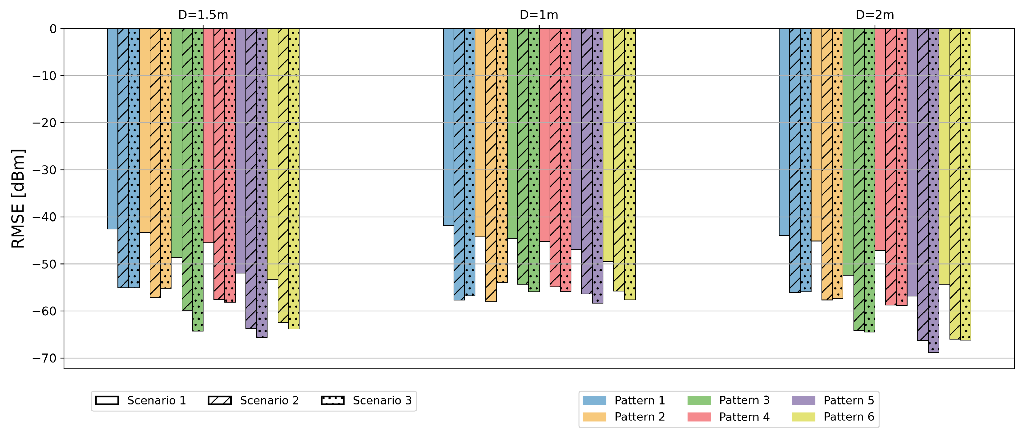
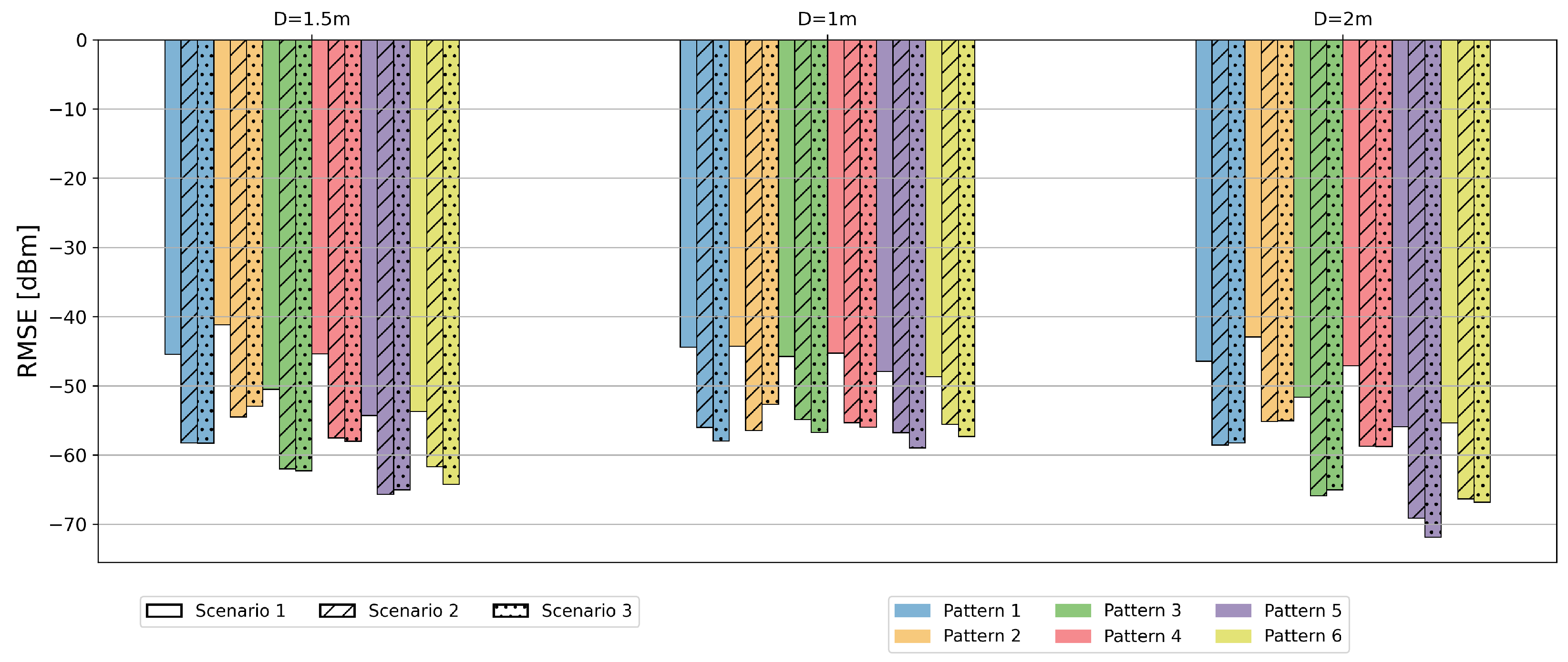
In order to assess the accuracy of the analyzed theoretical models for all conducted measurements, the values of the following metrics were calculated: root mean square error (RMSE) (8), mean absolute error (MAE) (9), and sum of squared differences (SSD) (10).

$$\mathrm{RMSE}=\sqrt{{\displaystyle \frac{1}{N}}\sum _{i=1}^N{\left(x_i-y_i\right)}^2},$$

(8)

$$\mathrm{MAE}={\displaystyle \frac{1}{N}}{\displaystyle \sum _{i=1}^N}|x_i-y_i|,$$

(9)

$$\mathrm{SSD}={\displaystyle \sum _{i=1}^N}(x_i-y_i{)}^2,$$

(10)

where $x_i$ and $y_i$ represent the i-th elements of the measured and theoretical data vectors of length N, respectively. In all cases, the received power values were substituted into the above formulas in the linear scale (expressed in mW). The resulting error metrics were subsequently converted to the decibel scale using the standard relation $E_{dB}=10{log}_{10}\left(E_{linear}\right)$ for presentation and comparison purposes. 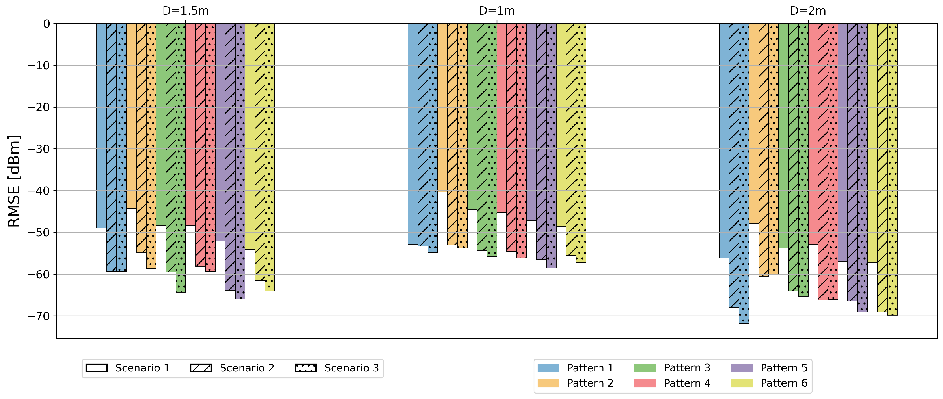For example, a calculated linear RMSE of ${10}^{-3}$ mW corresponds to $-30$ dBm in the reported results.Figure 7, Figure 8 and Figure 9 illustrate the RMSE variations for the three theoretical models across different radiation patterns and RIS–receiver distances. The corresponding averaged performance metrics—RMSE, MAE, and SSD—computed over all patterns for each measurement scenario are summarized in

Table 6. Performance metrics for Tang’s model (mean, median, and dispersion across patterns).

	Scenario 1			Scenario 2			Scenario 3
D =	1 m	1.5 m	2 m	1 m	1.5 m	2 m	1 m	1.5 m	2 m
RMSE (Mean) [dBm]	−44.82	−45.89	−47.73	−55.96	−58.34	−59.72	−56.17	−58.35	−59.71
RMSE (Median) [dBm]	−44.91	−46.80	−48.98	−56.06	−58.59	−60.65	−56.32	−60.08	−60.83
RMSE (IQR) [dB]	2.12	7.11	8.19	2.25	4.39	7.52	1.54	8.44	7.97
MAE [dBm]	−48.48	−49.98	−51.94	−59.59	−61.67	−63.74	−59.06	−62.08	−63.98
SSD [dBm2]	−71.65	−72.76	−76.03	−94.54	−98.16	−100.25	−94.87	−97.34	−99.98

,

Table 7. Performance metrics for Zheng’s model (mean, median, and dispersion across patterns).

	Scenario 1			Scenario 2			Scenario 3
D =	1 m	1.5 m	2 m	1 m	1.5 m	2 m	1 m	1.5 m	2 m
RMSE (Mean) [dBm]	−45.73	−45.98	−47.53	−55.75	−58.52	−59.70	−56.05	−58.01	−59.61
RMSE (Median) [dBm]	−45.47	−47.23	−48.78	−55.76	−59.61	−60.95	−56.97	−59.80	−60.84
RMSE (IQR) [dB]	2.64	7.23	7.48	0.97	4.26	7.61	1.67	5.60	7.90
MAE [dBm]	−49.18	−50.08	−51.77	−59.47	−61.86	−63.70	−59.00	−61.68	−63.84
SSD [dBm2]	−74.01	−71.87	−75.16	−94.41	−97.91	−99.47	−93.92	−95.73	−99.24

and

Table 8. Performance metrics for Jeong’s model (mean, median, and dispersion across patterns).

	Scenario 1			Scenario 2			Scenario 3
D =	1 m	1.5 m	2 m	1 m	1.5 m	2 m	1 m	1.5 m	2 m
RMSE (Mean) [dBm]	−44.88	−48.30	−52.76	−54.36	−58.58	−64.66	−55.76	−61.05	−65.13
RMSE (Median) [dBm]	−46.13	−48.67	−54.78	−54.41	−59.39	−66.28	−55.94	−61.11	−67.32
RMSE (IQR) [dB]	3.56	2.66	3.58	1.76	2.53	3.16	1.92	4.90	4.14
MAE [dBm]	−48.73	−52.37	−56.63	−58.39	−61.87	−68.25	−59.02	−64.08	−69.20
SSD [dBm2]	−70.24	−77.70	−85.66	−91.34	−98.41	−110.22	−93.94	−103.77	−109.94

for the Tang, Zheng, and Jeong models, respectively.

Despite visible discrepancies between the received power versus azimuth curves, the RMSE, MAE, and SSD metrics calculated for the three considered models yield very similar values. This indicates that on average, the models exhibit comparable error levels even if their detailed angular characteristics differ. In particular, the Tang and Zheng models produce nearly identical mean error values, while the Jeong model shows the highest initial errors at 1 m. It exhibits a much steeper reduction in error metrics as distance increases, eventually achieving the lowest RMSE and MAE values at 2 m compared to the Tang and Zheng models.

When considering the behavior across individual measurement scenarios, the observed trends remain consistent for all analyzed models. Scenario 3 (anechoic chamber with Metis antennas) provides the smallest errors, Scenario 2 (office with Metis antennas) follows, while Scenario 1 (office with Ainfo antennas) shows the largest discrepancies. The controlled chamber minimizes multipath, making the path loss models more accurate, whereas the office introduces distortions not captured by theory. The use of highly directional Ainfo antennas in Scenario 1 further amplifies the mismatch, since even small imperfections in RIS element behavior or alignment cause larger deviations, explaining the weakest agreement despite higher antenna gain.

A clear dependence on distance is observed across all models, but the rate of improvement varies. While Tang and Zheng models show a gradual decrease in error, the Jeong model’s accuracy improves with distance. This suggests that the Jeong model is particularly ill-suited for the very near-field (1 m), where element-specific geometry is critical, but it provides a very effective power envelope as the distance increases toward 2 m.

Table 6, Table 7 and Table 8 provide a detailed quantitative summary of the evaluated error metrics, including RMSE (Mean and Median), MAE, and SSD, calculated across all radiation patterns for each scenario. While the previous graphical analysis focused on general RMSE trends, the tabulated data allow for a deeper statistical investigation into the error distribution. The negative signs in Table 6, Table 7 and Table 8 reflect that the linear error magnitude is below the 1 mW reference level.

To better characterize model reliability both the mean and the median RMSE is presented. The median provides a more robust measure of the typical model performance by reducing the sensitivity to extreme outliers. Furthermore, the statistical dispersion is quantified using the Interquartile Range (IQR), which represents the spread of the middle 50% of the error distribution. In the logarithmic domain, the IQR is defined as:

$$IQR=10{log}_{10}\left(Q_3\right)-10{log}_{10}\left(Q_1\right),$$

(11)

where $Q_3$ and $Q_1$ are the 75th and 25th percentiles of the linear error values (in milliwatts), respectively.

Across all evaluated scenarios and models, a consistent trend is observed where the median RMSE is lower than the mean RMSE (with differences reaching up to 2.02 dB for the Jeong model in Scenario 3 at $D=2$ m). This confirms that the error distribution is positively skewed, primarily due to the influence of deep nulls in the radiation patterns.

Overall, the IQR for all evaluated models remains relatively low within specific scenarios, typically ranging between 0.97 and 8.44 dB. However, the Jeong model exhibits a higher overall dispersion across the full range of distances, indicating that while it can achieve lower errors at certain distances, its performance is less consistent. In contrast, the Tang and Zheng models provide a superior qualitative representation of the radiation lobes. By precisely calculating element-wise geometry, they attempt to track the physical oscillations of the signal, even though this leads to larger localized errors at pattern boundaries or in regions where phase-mismatches result in unphysical deep nulls. Ultimately, Tang’s and Zheng’s models offer a more authentic physical reconstruction of the RIS beamforming characteristics, whereas the Jeong model serves as a robust but simplified power estimator.

To verify whether the observed performance differences are statistically significant, a Wilcoxon signed-rank test was conducted. This non-parametric test was chosen over the parametric t-test due to the non-normal distribution of the RMSE values, which exhibit positive skewness caused by deep modeling nulls. Furthermore, the error values were rounded to the seventh decimal place prior to the test to ensure that numerical artifacts and floating-point precision errors did not lead to false significance in the comparisons.

The test compared the paired RMSE results across all evaluated cases (6 radiation patterns × 3 scenarios with 3 distances). The null hypothesis ($H_0$) assumed that there is no significant difference between the performance of the compared models. The results of the Wilcoxon signed-rank test, performed on the rounded data (${10}^{-7}$ mW precision), revealed two distinct outcomes:

• Jeong vs. Tang: $p=0.0195$ (statistically significant);
• Jeong vs. Zheng: $p=0.0763$ (no significant difference);
• Tang vs. Zheng: $p=0.4202$ (no significant difference).

The results of the Wilcoxon signed-rank test reveal a more nuanced relationship between the models. For the comparison between the Tang and Jeong models, the p-value ($p=0.0195$) is below the significance level ($\alpha =0.05$), allowing for the rejection of the null hypothesis and confirming that the performance difference between these two approaches is statistically significant. However, although the Jeong model achieves better metrics at 2 m, the test for the Zheng vs. Jeong comparison ($p=0.0763$) indicates that this advantage is not statistically significant across the entire dataset. This suggests that the Jeong model performs better at larger distances because its “smooth" approach avoids large errors on side lobes, but these gains are canceled out by its poor accuracy at 1 m, where ignoring the exact geometry of each element causes significant errors.

In contrast, the comparison between the Tang and Zheng models yielded $p=0.4202$. This indicates that these two models are statistically indistinguishable in the evaluated scenarios. This is a key finding, as it suggests that the sophisticated per-element amplitude mapping of the Zheng model does not provide a statistically superior result over the uniform amplitude approach of the Tang model, provided that both maintain high geometric precision for individual array elements.

5. Conclusions

This paper analyzes the accuracy of three popular RIS path loss models developed by Tang, Zheng, and Jeong. While all three models are widely recognized for their constructive insights into RIS-aided communications, this work verifies how their fundamental assumptions align with experimental data across diverse real-life scenarios. In summary, the Tang and Zheng models provide a high level of geometric precision by accounting for the individual coordinates and local reflection angles of each RIS element. Our analysis, supported by a Wilcoxon signed-rank test ($p=0.4202$), reveals that these two models are statistically indistinguishable. This suggests that the sophisticated element-wise amplitude mapping in the Zheng model does not offer a significant advantage over Tang’s uniform amplitude approach, provided that the precise geometry of the array is maintained. Both models excel at capturing the qualitative structure of the radiation patterns, including side-lobe oscillations, making them suitable for high-fidelity physical reconstructions. In contrast, the Jeong model prioritizes mathematical simplicity by employing a “central approximation” for the entire RIS surface. While this leads to the largest discrepancies in the immediate radiating near-field (1 m) where spherical wavefront effects are dominant, the model exhibits an improvement in accuracy as the distance increases. At 2 m, the Jeong model achieves the lowest average error metrics (RMSE, MAE, and SSD) by providing a smooth power envelope that effectively averages out signal oscillations. However, the lack of statistical significance in the Zheng vs. Jeong comparison ($p=0.0763$) and the higher global dispersion (IQR) of the Jeong model indicate that its superior performance at larger distances is partially offset by its lack of geometric precision at short ranges. Ultimately, these findings highlight a trade-off in RIS modeling: the Tang and Zheng models are more consistent and physically authentic across all distances, whereas the Jeong model serves as a robust, simplified power estimator that becomes increasingly effective as the receiver moves further into the radiating near-field.

The achieved results open the doors for further investigations. In essence, there is a need for proposing the way to reflect a particular environment in the RIS-aided propagation model. Our findings provide some guidelines regarding the typical office and are valid for a specific carrier frequency; however, there is a need for their generalization. It can be done by the introduction of some dedicated approximation coefficients that will depend on the surrounding environment. Moreover, it will be necessary to check and compare the accuracy of the models with other manufactured board types to draw more generalized conclusions. Finally, the results presented in this paper are associated with three specific distances; it will be highly beneficial to repeat the measurements to approximate the accuracy of the models as a function of the distance between the transmitter, receiver, and the RIS.