


A Lightweight Received Signal Strength Indicator Estimation Model for Low-Power Internet of Things Devices in Constrained Indoor Networks


Abstract
1. Introduction
- Implemented an RFR-based channel estimation method utilising Feature-based and Sequence-based strategies, demonstrating enhanced accuracy and efficiency for LP-IoT channel estimation.
- Conducted a comparative analysis against existing research and ANN-based methods, highlighting the substantial improvement in estimation error and training and testing time.
- Validated the lightweightness of developed RFR models over ANN-based models by deploying them on the Raspberry Pi 4 Model B platform.
2. Related Work
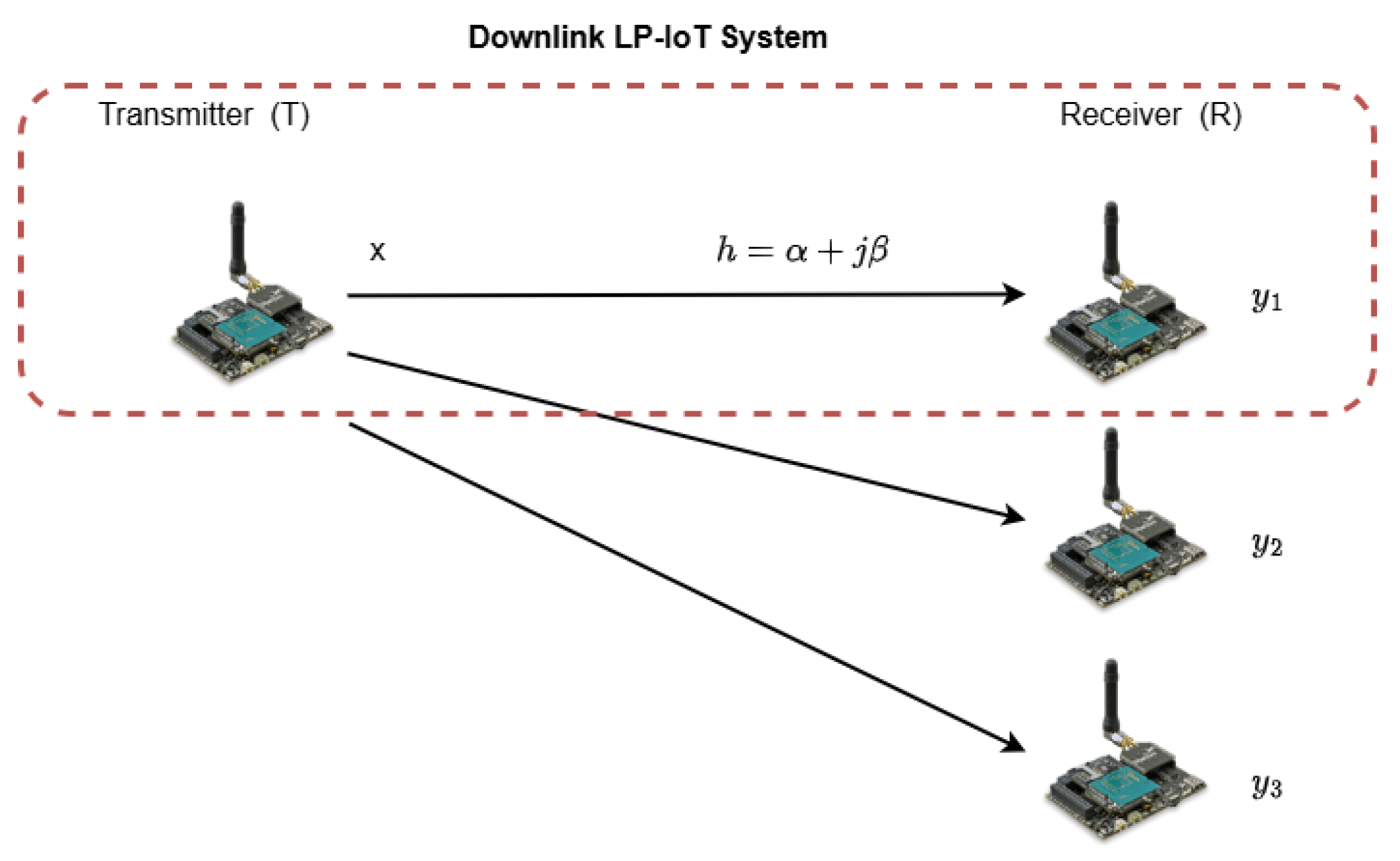
3. System Model
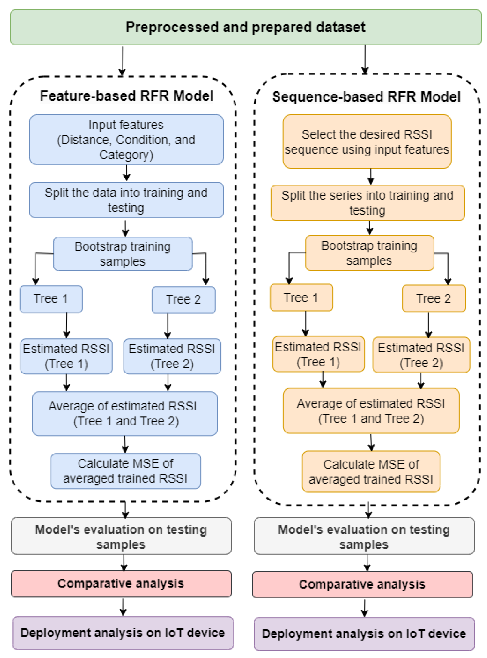
4. RFR-Based LP-IoT Channel Estimation Models
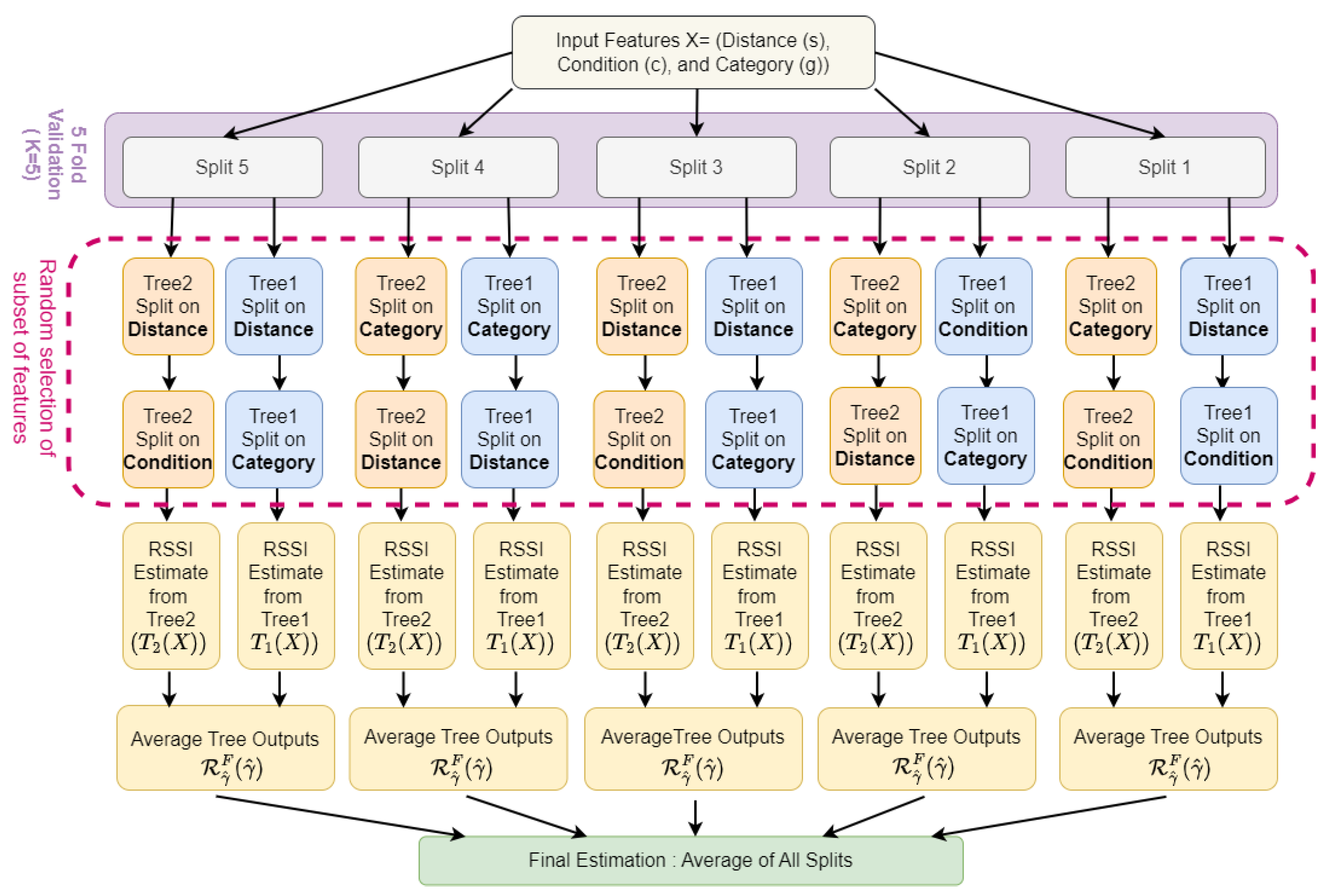
4.1. RFR(F) Model
Training and Evaluation
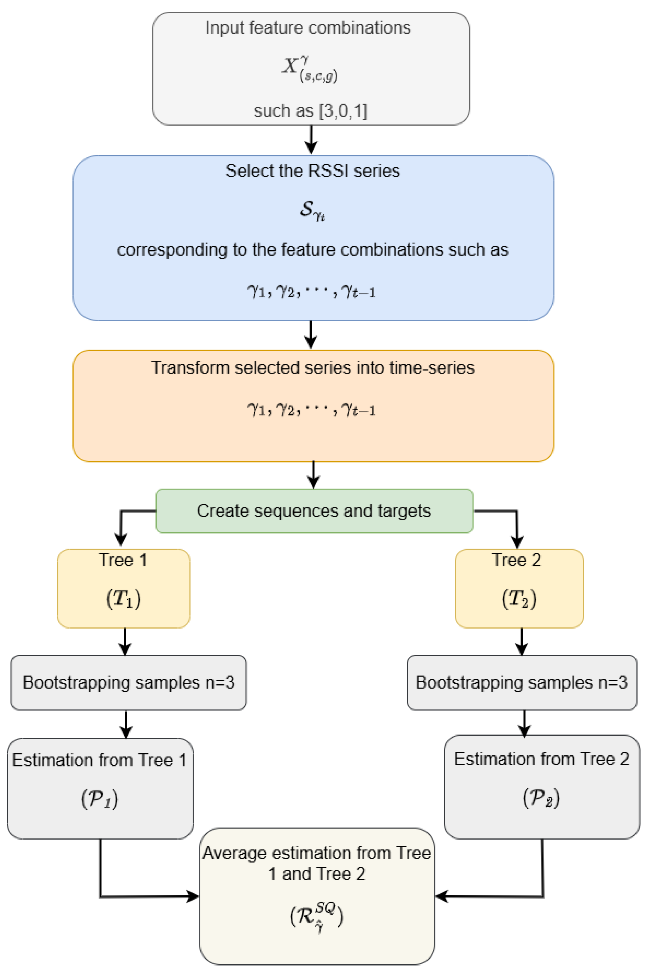
4.2. RFR(S) Model
Training and Evaluation
5. Deployment on LP-IoT Device
6. Results and Discussion
6.1. Estimation
6.2. Comparison
6.3. Complexity Analysis
7. Conclusions and Future Work
Author Contributions
Funding
Institutional Review Board Statement
Informed Consent Statement
Data Availability Statement
Acknowledgments
Conflicts of Interest
References
- Madakam, S.; Ramaswamy, R.; Tripathi, S. Internet of Things (IoT): A literature review. J. Comput. Commun. 2015, 3, 164. [Google Scholar] [CrossRef]
- Harsha, B.; Shalini, P.; Akhil, K.M. RSSI Based Pattern Classification in WSN Using Machine Learning. In Proceedings of the 2022 IEEE 7th International Conference on Recent Advances and Innovations in Engineering (ICRAIE), Mangalore, India, 1–3 December 2022; Volume 7, pp. 182–187. [Google Scholar]
- Dinev, D.; Haka, A. RSSI study of wireless Internet of Things technologies. J. Phys. Conf. Ser. 2022, 2339, 012014. [Google Scholar]
- Arif, S.; Khan, M.A.; Rehman, S. Wireless Channel Estimation for Low-Power IoT Devices Using Real-Time Data. IEEE Access 2024, 12, 17895–17914. [Google Scholar] [CrossRef]
- Rekkas, V.P.; Sotiroudis, S.P.; Koudouridis, G.P.; Sarigiannidis, P.; Zaharis, Z.D.; Karagiannidis, G.K.; Goudos, S.K. On the Accuracy and Efficiency of Received Signal Strength Modelling for a Forest Environment. In Proceedings of the 2024 IEEE International Conference on Machine Learning for Communication and Networking (ICMLCN), Stockholm, Sweden, 5–8 May 2024; pp. 399–404. [Google Scholar]
- Iwasaki, M.; Nishio, T.; Morikura, M.; Yamamoto, K. Transfer Learning-Based Received Power Prediction with Ray-tracing Simulation and Small Amount of Measurement Data. In Proceedings of the 2020 IEEE 92nd Vehicular Technology Conference (VTC2020-Fall), Victoria, BC, Canada, 18 November–16 December 2020; pp. 1–6. [Google Scholar]
- González-Palacio, M.; Tobón-Vallejo, D.; Sepúlveda-Cano, L.M.; Rúa, S.; Le, L.B. Machine-Learning-Based Combined Path Loss and Shadowing Model in LoRaWAN for Energy Efficiency Enhancement. IEEE Internet Things J. 2023, 10, 10725–10739. [Google Scholar] [CrossRef]
- Maduranga, M.; Abeysekara, R. Supervised machine learning for RSSI-based indoor localisation in IoT applications. Int. J. Comput. Appl. 2021, 183, 26–32. [Google Scholar]
- Arif, S.; Khan, M.A.; Rehman, S. Deep Learning Approaches to Indoor Wireless Channel Estimation for Low-Power Communication. In Proceedings of the 2024 IEEE International Conference on Communications Workshops (ICC Workshops), Denver, CO, USA, 9–13 June 2024; pp. 1547–1552. [Google Scholar]
- Saitoh, K. Deep Learning from the Basics: Python and Deep Learning: Theory and Implementation; Packt Publishing Ltd.: Birmingham, UK, 2021. [Google Scholar]
- Hu, Q.; Gao, F.; Zhang, H.; Jin, S.; Li, G.Y. Deep Learning for Channel Estimation: Interpretation, Performance, and Comparison. IEEE Trans. Wirel. Commun. 2021, 20, 2398–2412. [Google Scholar]
- Hoang, M.T.; Yuen, B.; Dong, X.; Lu, T.; Westendorp, R.; Reddy, K. Recurrent Neural Networks for Accurate RSSI Indoor Localisation. IEEE Internet Things J. 2019, 6, 10639–10651. [Google Scholar] [CrossRef]
- Ye, H.; Li, G.Y.; Juang, B.H. Power of Deep Learning for Channel Estimation and Signal Detection in OFDM Systems. IEEE Wirel. Commun. Lett. 2018, 7, 114–117. [Google Scholar]
- Debnath, S.; O’Keefe, K. Proximity Estimation with BLE RSSI and UWB Range Using Machine Learning Algorithm. In Proceedings of the 2023 13th International Conference on Indoor Positioning and Indoor Navigation (IPIN), Nuremberg, Germany, 25–28 September 2023; pp. 1–6. [Google Scholar]
- Biau, G.; Scornet, E. A random forest guided tour. Test 2016, 25, 197–227. [Google Scholar] [CrossRef]
- Rifki, M.I.; Ikhwan, A.; Muhammad, F. Performance Evaluation of RSSI Prediction Methods in Wireless Communication Networks. ZERO J. Sains Mat. Dan Terap. 2024, 8, 7–18. [Google Scholar] [CrossRef]
- Geis, M.; Sliwa, B.; Bektas, C.; Wietfeld, C. TinyDRaGon: Lightweight radio channel estimation for 6G pervasive intelligence. In Proceedings of the 2022 IEEE Future Networks World Forum (FNWF), Montreal, QC, Canada, 10–14 October 2022; pp. 658–663. [Google Scholar]
- Khan, K.; Iqbal, M.; Salami, B.A.; Amin, M.N.; Ahamd, I.; Alabdullah, A.A.; Arab, A.M.A.; Jalal, F.E. Application of Advanced Machine Learning and Artificial Neural Network Methods in Wireless Sensor Networks Based Applications. Int. J. Eng. Adv. Technol. 2022, 11, 103–109. [Google Scholar]
- Wang, Y.; Jia, Z.; Gan, R.; Li, J.; Xiao, Z. Evaluate Link Quality based on ISSA-BRF in Wireless Network. In Proceedings of the 2024 5th International Conference on Computing, Networks and Internet of Things, CNIOT ‘24, Tokyo, Japan, 24–26 May 2024; pp. 19–25. [Google Scholar]
- Azoulay, R.; Edery, E.; Haddad, Y.; Rozenblit, O. Machine learning techniques for received signal strength indicator prediction. Intell. Data Anal. 2023, 27, 1167–1184. [Google Scholar]
- Kumara, D.H.; Song, Z.; Rahmadya, B.; Kozume, S.; Sumiya, T.; Sun, R.; Takeda, S.; Wang, X. Indoor Area Estimation System Using RSSI-Measuring Handheld Reader Utilizing Directional Reference RFID Tags and Machine Learning. IEEE Access 2024, 12, 157872–157887. [Google Scholar]
- Aarif, L.; Tabaa, M.; Hachimi, H. RSSI prediction and optimisation of transmission power for improved LoRa communications performance. Ann. Telecommun. 2024, 1–20. [Google Scholar] [CrossRef]
- Ballestrin, R.; Feijó, J.F.; Feldman, M.; Müller, I. Exploring Machine Learning Techniques for Path Loss Prediction in LoRa Networks. In Proceedings of the 2024 19th International Symposium on Wireless Communication Systems (ISWCS), Rio de Janeiro, Brazil, 14–17 July 2024; pp. 1–6. [Google Scholar]
- Ramos, B.; Rosario, E.D.; Tovar, N. Assessing the Capability of Random Forest to Estimate Received Power in LoRaWAN for Agricultural Settings Using Climate Data. In Proceedings of the 2023 33rd International Telecommunication Networks and Applications Conference, Melbourne, Australia, 29 November–1 December 2023; pp. 234–239. [Google Scholar]
- Barrios-Ulloa, A.; Hoz-Franco, E.D.L.; Cama-Pinto, A. Comparison of machine learning path loss model for wireless sensor networks in cassava crops. In Proceedings of the 2023 IEEE Colombian Caribbean Conference (C3), Barranquilla, Colombia, 22–25 November 2023; pp. 1–6. [Google Scholar]
- Mallikarjun, S.B.; Kusumapani, S.C.; Kuruvatti, P.N.; Bhat, B.G.; Schotten, H.D. Machine Learning Based SINR Prediction in Private Campus Networks. In Proceedings of the 2023 IEEE 97th Vehicular Technology Conference (VTC2023-Spring), Florence, Italy, 20–23 June 2023; pp. 1–6. [Google Scholar]
- Dhama, S.; Akhtar, N.; Hathi, P.; Agnihotri, S. Downlink SNR Estimation of Wi-Fi Clients using Machine Learning. In Proceedings of the 2023 15th International Conference on COMmunication Systems NETworkS (COMSNETS), Bangalore, India, 3–8 January 2023; pp. 410–413. [Google Scholar]
- Kanto, Y.; Watabe, K. Wireless Link Quality Estimation Using LSTM Model. In Proceedings of the NOMS 2024—2024 IEEE Network Operations and Management Symposium, Seoul, Republic of Korea, 6–10 May 2024; pp. 1–5. [Google Scholar]
- Raj, N.; Vineeth, B. Indoor RSSINet-Deep learning based 2D RSSI map prediction for indoor environments with application to wireless localisation. In Proceedings of the 2023 15th International Conference on COMmunication Systems and NETworkS (COMSNETS), Bangalore, India, 3–8 January 2023; pp. 609–616. [Google Scholar]
- Arif, S.; Khan, M.A.; Rehman, S.; Abbas, S.M. RSSI Estimation for Constrained Indoor Wireless Networks Using ANN. In Proceedings of the 2024 International Conference on Electrical, Computer and Energy Technologies (ICECET), Sydney, Australia, 25–27 July 2024; pp. 1–6. [Google Scholar]
- Karthikeyan, S.; Raj, R.A.; Cruz, M.V.; Chen, L.; Vishal, J.L.A.; Rohith, V.S. A Systematic Analysis on Raspberry Pi Prototyping: Uses, Challenges, Benefits, and Drawbacks. IEEE Internet Things J. 2023, 10, 14397–14417. [Google Scholar] [CrossRef]


| Distance (s) (m) | Condition (s) 0 (LoS), 1 (NLoS) | Category (g) 0 (L1), 1 (L2 to L13), 2 (L14 to L40). | RSSI () (dBm) |
|---|---|---|---|
| 3 | 0 | 0 | −67.4 |
| 3 | 1 | 0 | −65.2 |
| 3 | 0 | 1 | −63 |
| 3 | 1 | 1 | −56 |
| 0.2 | 0 | 2 | −40 |
| 0.3 | 0 | 2 | −47 |
| 0.4 | 0 | 2 | −44 |
| 0.5 | 0 | 2 | −46 |
| 0.6 | 0 | 2 | −43 |
| 0.7 | 0 | 2 | −49 |
| 0.8 | 0 | 2 | −50 |
| 1.9 | 0 | 2 | −65 |
| 2 | 0 | 2 | −63 |
| Training | Testing | Training Time (s) | Testing Time (s) | ||
|---|---|---|---|---|---|
| MSE | RMSE | MSE | RMSE | ||
| Feature-based RFR(F) Estimation Model | |||||
| 3.16 | 1.77 | 3.20 | 1.79 | 0.0134 | 0.0010 |
| Feature-based ANN(F) Estimation Model [30] | |||||
| 5.91 | 2.43 | 5.30 | 2.30 | 87.2227 | 0.0040 |
| Current Research (TinyDRaGon Model) in [17] | |||||
| - | - | 5.15 | 2.27 | 600 | 45 |
| Current Research (Random Forest Model) in [24] | |||||
| - | - | 38.06 | 6.17 | - | - |
| Selected Sequence | Training | Testing | Training Time (s) | Testing Time (s) | ||
|---|---|---|---|---|---|---|
| MSE | RMSE | MSE | RMSE | |||
| Sequence-based RFR Estimation Model | ||||||
| [3, 0, 1] | 1.66 | 1.28 | 5.65 | 2.37 | 0.0010 | 0.0007 |
| [3, 1, 1] | 0.92 | 0.96 | 1.41 | 1.19 | 0.0008 | 0.0006 |
| [2, 0, 2] | 0.40 | 0.63 | 3.83 | 1.95 | 0.0007 | 0.0006 |
| [2, 1, 2] | 1.36 | 1.16 | 0.26 | 0.50 | 0.0008 | 0.0007 |
| [1, 0, 2] | 0.45 | 0.67 | 0.74 | 0.86 | 0.0008 | 0.0006 |
| [1, 1, 2] | 3.11 | 1.76 | 2.90 | 1.70 | 0.0014 | 0.0008 |
| [0.5, 0, 2] | 0.43 | 0.66 | 0.79 | 0.89 | 0.0006 | 0.005 |
| [0.5, 1, 2] | 0.55 | 0.74 | 0.34 | 0.58 | 0.0010 | 0.0011 |
| Sequence-based ANN Estimation Model [30] | ||||||
| [3, 0, 1] | 2.94 | 1.71 | 9.40 | 3.06 | 0.7091 | 0.0006 |
| [3, 1, 1] | 1.23 | 1.11 | 1.51 | 1.23 | 0.4962 | 0.0005 |
| [2, 0, 2] | 0.91 | 0.95 | 4.36 | 2.08 | 0.369 | 0.0009 |
| [2, 1, 2] | 2.86 | 1.69 | 0.35 | 0.59 | 0.360 | 0.0010 |
| [1, 0, 2] | 0.94 | 0.96 | 1.57 | 1.25 | 0.422 | 0.0005 |
| [1, 1, 2] | 10.13 | 3.18 | 2.37 | 1.54 | 0.4804 | 0.0018 |
| [0.5, 0, 2] | 0.90 | 0.95 | 1.43 | 1.19 | 0.739 | 0.0005 |
| [0.5, 1, 2] | 1.45 | 1.20 | 0.21 | 0.46 | 0.381 | 0.0004 |
| Current Research (TinyDRaGon Model) in [17] | ||||||
| - | - | - | 10.24 | 3.20 | - | - |
| Current Research (Random Forest Model) in [24] | ||||||
| - | - | - | 38.06 | 6.17 | - | - |
| LP-IoT Deployment Platform-Raspberry Pi Model B | ||||
|---|---|---|---|---|
| Analysis Phase | Training | Testing | ||
| Complexity Parameters | Memory Usage (MBs) | CPU Utilisation (%) | Memory Usage (MBs) | CPU Utilisation (%) |
| Feature-based RFR Model | 923 | 2.1 | 925 | 1.27 |
| Feature-based ANN Model | 1095.68 | 99.25 | 1095.68 | 7.65 |
Disclaimer/Publisher’s Note: The statements, opinions and data contained in all publications are solely those of the individual author(s) and contributor(s) and not of MDPI and/or the editor(s). MDPI and/or the editor(s) disclaim responsibility for any injury to people or property resulting from any ideas, methods, instructions or products referred to in the content. |
© 2025 by the authors. Licensee MDPI, Basel, Switzerland. This article is an open access article distributed under the terms and conditions of the Creative Commons Attribution (CC BY) license (https://creativecommons.org/licenses/by/4.0/).
Share and Cite
Arif, S.; Khan, M.A.; Rehman, S.u. A Lightweight Received Signal Strength Indicator Estimation Model for Low-Power Internet of Things Devices in Constrained Indoor Networks. Appl. Sci. 2025, 15, 3535. https://doi.org/10.3390/app15073535
Arif S, Khan MA, Rehman Su. A Lightweight Received Signal Strength Indicator Estimation Model for Low-Power Internet of Things Devices in Constrained Indoor Networks. Applied Sciences. 2025; 15(7):3535. https://doi.org/10.3390/app15073535
Chicago/Turabian StyleArif, Samrah, M. Arif Khan, and Sabih ur Rehman. 2025. "A Lightweight Received Signal Strength Indicator Estimation Model for Low-Power Internet of Things Devices in Constrained Indoor Networks" Applied Sciences 15, no. 7: 3535. https://doi.org/10.3390/app15073535
APA StyleArif, S., Khan, M. A., & Rehman, S. u. (2025). A Lightweight Received Signal Strength Indicator Estimation Model for Low-Power Internet of Things Devices in Constrained Indoor Networks. Applied Sciences, 15(7), 3535. https://doi.org/10.3390/app15073535