Article

Hybrid ML/DL Approach to Optimize Mid-Term Electrical Load Forecasting for Smart Buildings

1
Department of Engineering and Applied Sciences, University of Bergamo, 24044 Bergamo, Italy
2
Department of Engineering, University of Sannio, 82100 Benevento, Italy
3
Department of Civil, Construction-Architectural and Environmental Engineering, University of L’Aquila, 67100 L’Aquila, Italy
4
Department of Energy, Systems, Territory and Construction Engineering (DESTEC), University of Pisa, Largo Lucio Lazzarino 1, 56122 Pisa, Italy
5
Department of Digital and Innovation, ABB SACE S.p.A., 24123 Bergamo, Italy
*
Author to whom correspondence should be addressed.
Appl. Sci. 2025, 15(18), 10066; https://doi.org/10.3390/app151810066
Submission received: 1 August 2025 / Revised: 7 September 2025 / Accepted: 9 September 2025 / Published: 15 September 2025
(This article belongs to the Special Issue Advanced Methods for Time Series Forecasting)

Abstract

Most electric energy consumption in the building sector is provided by fossil fuels, leading to high greenhouse gas emissions. However, the increasing need for sustainable infrastructure has triggered a significant trend toward smart buildings, which enable optimal and efficient resource usage. In this context, accurate mid-term energy load forecasting is crucial for energy management. This study proposes a hybrid forecasting model obtained through the combination of machine learning (ML) and deep learning (DL) approaches designed to enhance forecasting accuracy at an hourly granularity. The hybrid two-layer architecture first investigates the model’s performance individually, such as decision tree (DT), random forest (RF), support vector regression (SVR), Extreme Gradient Boosting (XGBoost), FireNet, and long short-term memory (LSTM), and then combines them to leverage their complementary strengths in a two-layer hybrid design. The performance of these models is assessed on smart building energy datasets with weather data, and their accuracy is measured through performance metrics such as mean squared error (MSE), root mean squared error (RMSE), and R-squared ( R 2 ). The collected results show that the XGBoost outperformed other ML models. However, the hybrid model obtained by combining FireNet and XGBoost models delivers the highest overall accuracy for the performance parameters. These findings highlight the effectiveness of hybrid models in terms of prediction accuracy. This research contributes to reliable energy forecasting and supports environmentally sustainable practices.

1. Introduction

The expansion of the urban population and rising living standards have significantly increased energy consumption and shifted demand patterns, placing substantial stress on conventional energy infrastructure [1,2]. According to the International Energy Agency (IEA), buildings account for about 38% of total energy use in urban settings and about 40% of carbon emissions [3]. Globally, the building sector accounts for roughly one-third of energy consumption and one-quarter of CO2 emissions, These figures highlight the sector’s energy intensity and its considerable influence on global greenhouse gas (GHG) emissions.
The intensive use of fossil fuels and their environmental impacts have contributed to climate extremes in recent years, prompting the scientific community to pursue environmentally friendly technologies [4,5]. The adoption of renewable energy, particularly solar and wind, has underpinned the transition toward a sustainable future [6]. However, the intermittent nature of these sources, together with the need for robust forecasting to ensure power-system stability [7], poses tangible challenges for grid operators. In this context, accurate and timely forecasting of building energy consumption is essential for grid reliability, optimizing resource use, and minimizing both operational costs and environmental impacts [8].
Energy forecasting in buildings enables informed decisions on energy procurement, load balancing, and demand-side management [9,10]. Because historical operational data are lacking at new construction sites, simulations are commonly used; for existing buildings, data-driven methods offer faster and more accurate predictions. Traditional statistical methods such as autoregressive integrated moving average (ARIMA) and linear regression have served as baselines, but their limited capacity to model nonlinearity often hampers performance, especially in complex environments. By contrast, machine learning (ML) and deep learning (DL) algorithms offer powerful alternatives that handle high-dimensional, non-linear datasets with greater accuracy and adaptability [11]. Research findings highlight the growing importance of intelligent energy forecasting systems that exploit weather data (e.g., temperature, humidity, and solar irradiance) to enhance forecasting accuracy [12]. Indeed, weather variables play a key role in building energy performance, and their inclusion in forecasting algorithms can yield 15–30% savings compared with deterministic, non-weather sensitive approaches. Smart metering systems and the Internet of Things (IoT) are recent developments that enable more efficient energy management [13]. Continuous data acquisition provided by smart metering systems enables forecasting models to learn from dynamic consumption behavior and environmental conditions in near real-time [14]. This capability supports user-centric operation and cost-effective solutions, both of which are pivotal for a sustainable future.
Despite these advancements, challenges remain in model generalization, data heterogeneity, and effective feature selection factors critical for deploying scalable, transferable solutions. A variety of ML and DL techniques have been explored for building energy forecasting. In particular, random forest (RF), support vector regression (SVR), artificial neural networks (ANNs), and extreme learning machines (ELM) are common ML algorithms, while convolutional neural networks (CNNs), long short-term memory (LSTM) networks, and hybrid architectures are gaining attention in the DL domain [15,16,17,18]. A brief introduction to these techniques is provided in Section 2. However, many existing studies are restricted to specific regions and lack reproducibility across different climates or structural configurations. Moreover, most available literature focuses on short-term prediction, where the restricted forecasting horizon (e.g., 24 h) limits flexibility for energy management applications.
In this work, we develop a scalable data-driven framework for forecasting building energy consumption using ML, DL, and hybrid models. The methodology is applied to a smart, multi-story commercial building that uses both conventional grid electricity and on-site solar energy. Electrical power consumption data were collected using smart circuit breakers and communication devices integrated with a cloud infrastructure. Additionally, meteorological data including temperature, irradiance, wind speed, and humidity were sourced from NASA’s POWER database [19] and synchronized with the energy records to capture environmental dependencies. Feature selection was guided by correlation analysis, and multiple ML and DL algorithms were implemented and compared using standard performance metrics, including measures of computational efficiency. Unlike most prior studies that focus on short-term horizons or single-method approaches, this study introduces a hybrid framework that integrates ML and DL models to improve mid-term, hourly forecasting accuracy. The inclusion of both building consumption and weather variables, applied to a smart building with integrated renewable energy, reinforces the originality and practical relevance of the proposed approach.
Key features of the proposed methodology are the following:
  • The capability to model building energy consumption based on grid power.
  • Integration of high-resolution energy and meteorological data.
The objective of this study is to develop and evaluate a scalable hybrid forecasting framework that integrates ML and DL algorithms for mid-term, hourly energy load prediction in smart buildings. The analysis considers fundamental variables such as electrical consumption data, meteorological factors (temperature, irradiance, wind speed, humidity), and standard performance indicators (MSE, RMSE, R 2 ). By explicitly incorporating these variables, the study provides a comprehensive evaluation of forecasting accuracy and practical utility in sustainable energy management.
The paper is structured as follows. Section 2 reviews related literature on energy forecasting using ML, DL, and hybrid techniques, highlighting key methodologies and research gaps. Section 3 outlines the proposed method, including data acquisition, feature selection, hyper-parameter tuning, cross-validation, and model development strategies. Section 4 presents simulation results, comparing individual ML/DL models and hybrid approaches across several evaluation metrics. Section 5 concludes with key findings.

2. Literature Review

Given their dominant share in energy use and emissions, buildings have become a primary focus in the development of sustainable and intelligent energy systems [20]. As energy efficiency becomes a global priority, accurate energy demand forecasting is essential not only for optimizing management strategies but also for reducing operational costs and enhancing environmental outcomes.
For existing buildings with time-series energy data, ML techniques have demonstrated reliable performance in consumption forecasting, effectively capturing non-linearities and variable interactions. Using daily data granularity with RF and SVR has been shown to improve accuracy compared with weekly aggregation [21]. Comparative studies further report that ensemble approaches generally outperform individual models such as ANN, SVR, CART, LR, and SARIMA [22]. The importance of selecting an appropriate forecasting model is emphasized in [23]; common ML choices include RF, ELM, and SVR, as summarized in Table 1. In addition to model selection, recent studies highlight that prediction accuracy is strongly influenced by combining multiple data sources. Historical load, meteorological variables, temporal features (e.g., hour, weekday, season), and occupancy information together form robust feature sets for learning.
DL methods, including LSTM networks and CNNs, show strong potential for modeling complex temporal dependencies in energy data, particularly when large-scale datasets and long sequential patterns are available. LSTM has been applied to long-term building load forecasting by leveraging periodic usage patterns [24], while CNN-based architectures such as FireNet achieved high accuracy when incorporating environmental parameters like weather [25]. As summarized in Table 1, DNN and CNN-LSTM models have also been deployed in contexts such as university campuses and benchmark datasets [26], yielding accurate results when trained with weather, occupancy, and power-related features. A wavelet–neural network approach reduced prediction errors and improved energy efficiency (8%) while accurately forecasting CO2 emissions, underscoring machine learning’s role in smart building management [27].
Hybrid models that combine ML and DL techniques, or multiple DL layers, have emerged as robust forecasting solutions. For instance, the RF–IPWOA–ELM model integrates RF for feature selection, the Improved Parallel Whale Optimization Algorithm (IPWOA) for hyper-parameter tuning, and ELM for prediction, achieving up to 25% improvements over DT and 5.5% over SVR in cooling-load forecasting [28]. Similarly, CNN–LSTM frameworks predict residential energy consumption by combining CNN layers for spatial feature extraction with LSTM layers for temporal dynamics [29]. Other combinations, including LSTM–XGBoost and LSTM–RF, have also been adopted to jointly capture long-term temporal dependencies and non-linear feature interactions, yielding superior accuracy in mid-term forecasting tasks [30]. A hybrid deep learning model integrating CNN, Bi-LSTM, GNN, and Transformer with a Fusion Layer enhanced feature extraction, temporal and spatial learning, and attention-based trend detection, leading to more accurate energy load forecasting for smart cities [31]. An advanced electrical load forecasting framework combining improved feature extraction method, and a hybrid ANN–LSTM model has been proposed. This model achieves more accurate and robust forecasts, supporting effective energy management and planning [32]. Recent literature further highlights that the effectiveness of such hybrid frameworks depends not only on the learning architecture but also on the integration of diverse features, where historical load is combined with meteorological and temporal inputs to strengthen forecasting performance.
Recent literature also highlights the integration of emerging deep learning paradigms such as transfer learning and attention mechanisms, which are reshaping forecasting strategies for energy prediction tasks. Transfer learning has shown particular promise for adapting models across buildings with varying characteristics or limited data availability. For instance, ref. [33] proposed a multi-source transfer learning approach with LSTM and domain adaptation, enabling cross-building knowledge transfer and improved generalization performance. Attention-based methods are also gaining momentum for their ability to emphasize temporally significant inputs. In this context, ref. [34] developed an attention-enhanced sequence-to-sequence model that incorporates transfer learning to forecast building energy consumption under diverse climatic and regional settings. Similarly, ref. [35] conducted a systematic review of DL-based forecasting models, noting the increasing use of attention layers and hybrid deep neural networks to enhance interpretability and performance in complex urban energy systems. These advancements reinforce the shift toward modular, intelligent forecasting architectures that are both data-efficient and scalable, making them highly suitable for deployment in real-world smart building scenarios.
Table 1 shows the trend toward hybrid architectures, including techniques like kernel-based convolutional neural network (KCNN)–LSTM and model stacking, which demonstrates a growing emphasis on combining spatial, temporal, and contextual features for enhanced predictive performance.
Existing research on energy load forecasting has mainly concentrated on either short-term predictions, such as day-ahead forecasting, or long-term trends, while often neglecting the mid-term range, especially weekly to monthly forecasting at hourly resolution. This mid-term focus is important for effective planning in decentralized energy systems [21]. Many previous studies also use limited input features, usually relying only on past energy usage and basic weather data, without including more detailed factors like holidays, seasons, building schedules, or occupancy information [26]. Although some hybrid models combining machine learning (ML) and deep learning (DL) have been explored, few are designed to handle both long-term patterns and complex data interactions. In addition, these models are rarely compared with strong single-model baselines, which limits the ability to evaluate their true performance [29]. Another key issue is how these models are validated. Many studies still use random k-fold cross-validation, which can lead to information leakage across time and give overly optimistic results [36].
Table 1. Review of ML, DL, and hybrid techniques in load forecasting, highlighting gaps in feature sets and forecast horizons.
Ref.DatasetFrequencyFeaturesModelsKey FindingsLimitations
[21]Educational buildingsHourlyEnergy usage behaviorRF, RT, SVRML methods provide accurate hourly forecasts in educational buildings.Restricted to two buildings; no DL/hybrid comparison.
[22]Residential smart gridDailyUsage patternsANN, SVR, CART, LR, SARIMAComparative daily forecasting shows ML superiority over statistical models.Daily horizon only; potential over-fitting issues.
[26]University campusHourlyOperations, HVACDNN, RF, SVM, GBTDNN with engineered HVAC features improves accuracy.Relies on engineered HVAC variables; no hybrid approaches.
[28]Commercial buildingsHourly, MonthlyCooling load factorsRF, IPWOA, ELMHybrid RF–IPWOA–ELM enhances cooling load prediction.Focused only on cooling load; limited generalization.
[29]UCI RepositoryHourlyVoltage, occupancy, powerCNN–LSTMCNN–LSTM outperforms classical baselines in smart meter data.Based on a single household; no weather variables.
[30]Residential buildingsYearlyWeather, occupancy, designANN, DNN, RF, KNN, SVMDNN provides robust performance for annual load forecasting.Annual horizon; lacks short/medium-term forecasting detail.
[37]Utility dataHourlyWeather + power demandRFRF achieves low day-ahead forecast errors.System-level forecasting; not building-specific.
[36]Cooling load dataHourlyEnv. factors, occupancySVRSVR with environmental variables enhances prediction accuracy.Limited to summer season; one office building only.
[38]Hospital energy dataDailyLoad consumptionXGBoost, RFEnsemble methods outperform individual learners for hospital load.No DL or hybrid models tested.
[39]Mixed datasetsHourlyUsage and weatherSVR, LSTMSVR achieves comparable or better results than LSTM.Narrow scope of hybrid testing; dataset heterogeneity challenges.
[40]Commercial building15-minTimestamp + loadKCNN–LSTMCombining clustering with DL improves short-term forecasts.Limited exogenous features; scalability uncertain.
[33]Multiple building types (Japan)HourlyHistorical load, weatherLSTM + Multi-source Transfer Learning (MK-MMD)Multi-source domain adaptation improves performance vs. single-source transfer.Requires domain similarity; complex setup.
[34]Green buildings (China)DailyHistorical consumption, temp., humiditySeq2Seq + Attention + Transfer LearningAttention-guided TL model forecasts accurately across climate zones.Model needs careful tuning; limited to similar use cases.
Also, most research does not test model performance across different seasons or building types, making it hard to apply the results in real-world settings [37]. Most evaluations focus only on basic accuracy metrics like RMSE or MAPE, while ignoring important factors such as uncertainty in predictions, how fast the model runs, or how often it needs retraining [28]. More recent studies have started to address some of these challenges by using transfer learning and attention mechanisms to improve model adaptability and accuracy [33,34]. These techniques help models work well across different buildings and focus on the most important parts of the data. However, their use in mid-term forecasting at hourly resolution is still limited, which supports the need for the hybrid approach proposed in this work.
To address these gaps, this study proposes a hybrid ML–DL framework that integrates environmental, temporal, and operational features for mid-term hourly forecasting in smart buildings. The approach is evaluated using robust, time-aware validation protocols and is benchmarked against strong ML and DL baselines to demonstrate its practical relevance and modeling advantages.

3. Methodology

3.1. Data Description and Analysis

The effectiveness of a forecasting system fundamentally depends on two primary components: the integrity of the input data and the forecasting mechanism. Therefore, a comprehensive approach to data collection and cleansing was implemented. Electrical power consumption data were collected through intelligent circuit breakers, communication devices, and a cloud database in a smart commercial building in Bergamo, Italy. The facility covers approximately 30,000 m2 and integrates advanced energy management systems. It includes multiple office spaces, laboratories, and production areas, accommodating several hundred employees. The hourly electrical load data span a three-year period from January 2021 to December 2023. Each yearly dataset consists of 8760 records (rows) and 11 features (columns), including the timestamp and electrical parameters such as the average, minimum, and maximum values of active power ( P Avg , P Min , P Max ), reactive power ( Q Avg , Q Min , Q Max ), and apparent power ( S Avg , S Min , S Max ). These values were obtained through hourly measurements collected continuously over a 12-month period [41]. An example of the data structure is presented in Table 2.
Table 3 illustrates a dataset with five entries of non-linear weather parameters for 2021, namely beam irradiance (Gb(i)), diffuse irradiance (Gd(i)), sunshine duration (H_sun), air temperature at 2 m (T2m), and wind speed at 10 m (WS10m). These data were sourced from the NASA Prediction of Worldwide Energy Resource (POWER) [42], which provides quality global meteorological and climate data appropriate for various research applications. The weather data are notably valuable for examining the influence of meteorological aspects on energy usage in smart commercial structures and estimating possible energy production. Table 2 and Table 3 were merged to synchronize time stamps, namely date, hour, day, month, and year for each record. These datasets were employed for examination and determining how changes occurred across the years. The dataset was split chronologically into training (70%), validation (15%), and testing (15%) sets, without shuffling, to prevent temporal leakage.
The electrical load data is systematically organized by date and the seasonal index, as presented in Table 4. This classification helps structure the data for identifying patterns across different calendar scenarios and seasonal trends. The indexes represent standard working days, typically Monday to Friday, excluding recognized public holidays. An additional index broadens the analysis to include weekends and holidays, thereby capturing a more extensive range of consumption behaviors. Further indexes encompass statistical aggregations of daily, weekly, and monthly averages, while also emphasizing the significance of seasonal categorization. This methodical classification allows for a thorough temporal segmentation, thereby enhancing the precision of modeling and analysis of load patterns that are influenced by human activities and institutional timetables. Figure 1 illustrates active power-consumption patterns at four temporal resolutions (hourly, daily, weekly, and monthly) captured from a smart commercial building. The analysis is based on power consumption from the electrical grid, excluding on-site renewable generation. These visualizations are essential for understanding energy consumption behavior and identifying temporal patterns that inform the design of forecasting models. The daily resolution plot reveals wide interquartile ranges and frequent outliers, indicating irregular consumption, likely driven by operational anomalies or peak demand events. This variability emphasizes the importance of forecasting frameworks capable of handling noise and capturing outlier behavior. At the hourly resolution (Figure 1a), a clear diurnal load cycle is evident, with demand increasing in the morning and peaking between mid-morning and early afternoon.
Following 16:00, consumption decreases sharply, reflecting reduced occupancy and operational activity. Such granularity is critical for short-term load prediction tasks. Figure 1c shows higher median loads on weekdays compared with weekends, a trend characteristic of commercial operations. Week-to-week fluctuations may be attributed to external influences such as holidays, weather conditions, or partial building usage, which introduce short-term non-stationarity into the data. The monthly resolution captures broader seasonal trends, as shown in Figure 1d. Although overall consumption is relatively consistent, some months show elevated averages, likely due to greater HVAC use or seasonal shifts in operational intensity. Together, these multi-resolution visual insights provide a comprehensive view of energy behavior across timescales. Incorporating such temporal diversity in input features can enhance the adaptability and predictive power of ML and DL models in energy forecasting. Two additional visualizations were created to further analyze power consumption behavior across multiple temporal resolutions. Figure 2a displays hourly power usage across the year 2023, highlighting significant intra-day and seasonal variations. Peak demands are especially noticeable during the mid-year months, likely driven by increased cooling requirements in summer. This fine-grained view of hourly data is crucial for capturing daily load cycles and informing real-time energy management decisions. As illustrated in Figure 2b, daily, weekly, and monthly average consumption trends for 2023 are also presented to reflect different temporal perspectives. The line representing daily averages exhibits high frequency fluctuations, capturing short-term variability. The weekly average smooths these fluctuations, revealing medium-term behavioral consistency, while the monthly average highlights broader seasonal trends. This layered averaging technique is valuable for distinguishing between transient and structural patterns in energy demand. Together, Figure 2 provides a comprehensive view of energy usage dynamics, serving as a foundational reference for the forecasting model’s design and effective load management strategies.
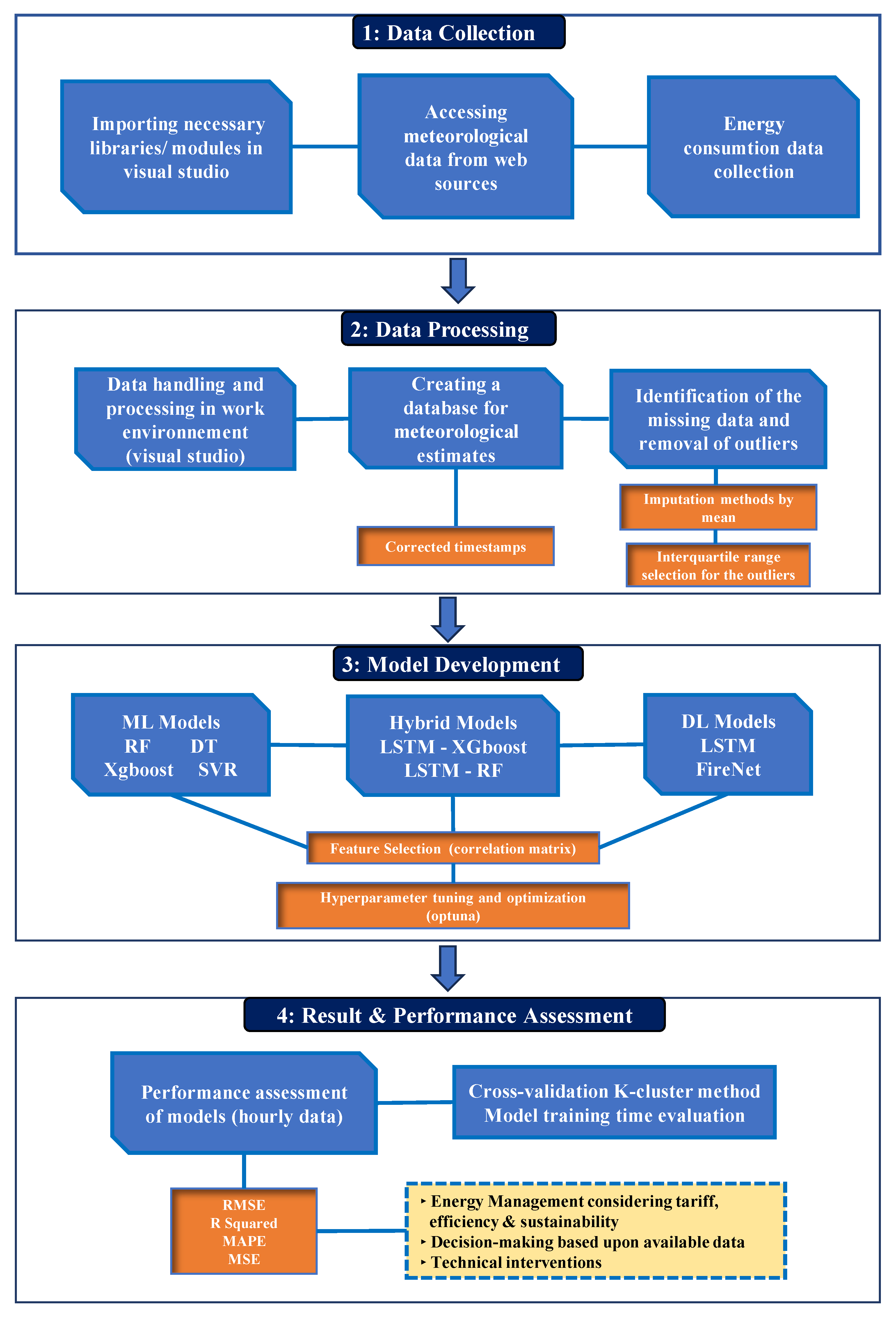
In Figure 3, forecasting process begins with the acquisition of hourly energy consumption data alongside relevant meteorological variables. Preprocessing is then applied to address missing values, construct informative features, and normalize the dataset. In the modeling phase, both ML algorithms (XGBoost, RF, SVR, DT) and DL architectures (LSTM, FireNet) are developed independently and in hybrid configurations. Performance evaluation follows, utilizing standard metrics such as RMSE, MAPE, and  R 2 to identify the most accurate and computationally efficient approach.

3.2. Feature Selection

The correlation coefficient r is given by Equation (1), where x i and y i denote individual values of variables x and y, respectively, and  x ¯ , y ¯ are their corresponding means [43].
r = ( x i x ¯ ) ( y i y ¯ ) ( x i x ¯ ) 2 ( y i y ¯ ) 2
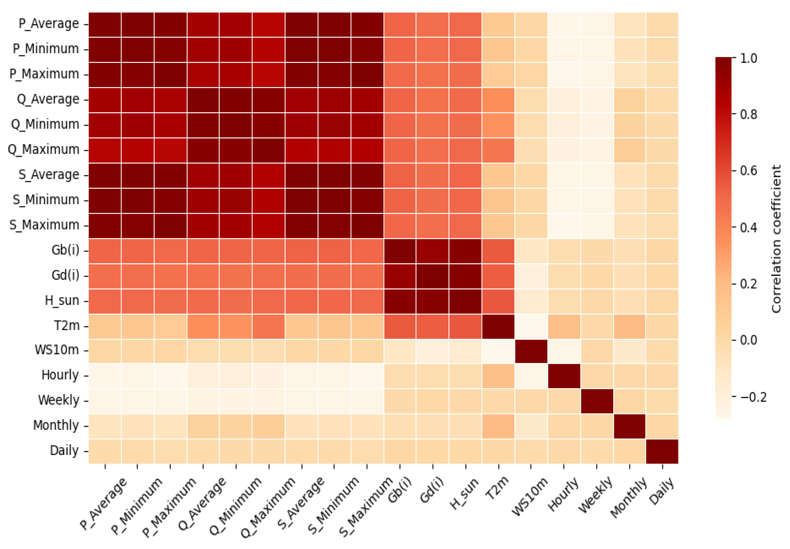
This metric was applied to measure the strength of the relationship between each input feature and the target variable P avg , as well as to detect high intercorrelation among variables. Figure 4 displays the Pearson correlation matrix heatmap for electrical and meteorological variables. Features showing strong correlation with the target variable, typically ranging from 0.29 to 0.88, were retained. Highly correlated power features, including P_Minimum, and P_Maximum, were considered redundant and consolidated into a single representative: P avg . Similarly, from the reactive and apparent power groups, only one representative linear feature ( Q avg ) was selected to reduce model bias and the risk of over-fitting. The non-linear features retained for modeling included meteorological variables such as air temperature at 2 m (T2m), sunshine duration (H_sun), solar irradiance (Gb(i) and Gd(i)), and wind speed at 10 m (WS10m). Wind speed exhibited a weak correlation with the target variable and was excluded. This feature selection strategy balances model complexity and generalization while maintaining computational efficiency.

3.3. Machine Learning Models

RF is an ensemble learning technique that builds multiple decision trees using random subsets of features and samples, then averages predictions. This approach enhances stability and accuracy, especially for complex, non-linear problems. RF handles both categorical and continuous variables and includes a built-in feature-importance measure [44]. In energy forecasting, RF has been applied to load prediction and has outperformed several conventional ML models in accuracy [45]. For example, in [21], RF was used to forecast hourly energy consumption in buildings, demonstrating high accuracy and efficient parameter tuning. DTs, particularly Classification and Regression Trees (CART), form the basis of many ensemble methods. They recursively split input data into branches and leaf nodes that represent outcomes. DTs are interpretable and can effectively model non-linear patterns, though they may over-fit to noisy data. As discussed in [46], ensemble strategies such as RF and Gradient Boosted Trees (GBT) are commonly used to overcome this limitation. DTs have also been used in hybrid models for energy forecasting tasks, including short-term load prediction and fuzzy rule-based classification [47].
SVR is a supervised ML framework designed for regression tasks, where the target variable is continuous rather than discrete. It estimates a regression function within a margin of tolerance, using kernel functions to capture complex relationships in data [48]. This enables SVR to identify non-linear relationships while preserving the dimensionality of the feature space. Furthermore, its capacity to mitigate over-fitting through regularization enhances its robustness to datasets with noise or uncertainty [49]. XGBoost is a powerful implementation of gradient boosting that sequentially adds weak learners to minimize residual error [50]. It includes regularization to reduce over-fitting and can handle sparse or missing data. XGBoost has been widely adopted in forecasting due to its speed and accuracy. For example, it has been combined with Gaussian mixture clustering to capture behavioral patterns in household energy forecasting [51].

3.4. Deep Learning Models

LSTM networks have emerged as powerful tools for time-series prediction tasks in the energy domain due to their ability to learn long-range temporal dependencies. In this study, the LSTM model is implemented as a baseline DL approach to forecast hourly energy consumption patterns of a smart commercial building. The architecture employs multiple hidden layers and memory cells, enabling the model to retain temporal context, essential for capturing diurnal and weekly variations in power demand. The LSTM model is fine-tuned using dropout regularization and a sequence-to-one prediction strategy to reduce over-fitting and improve generalization on unseen hourly data.
The FireNet model [52] is a DL architecture composed of five convolutional layers, each followed by max-pooling operations. Initially developed for image classification, FireNet is here used for time-series forecasting of building energy consumption. This adaptation leverages its hierarchical feature extraction capabilities to capture complex temporal dependencies. The model processes sequential input data through successive convolutional layers, each extracting temporal patterns at different scales. With 32 filters, the first layer captures short-term fluctuations such as hourly demand spikes. The input matrix is given by Equation (2), where T denotes the number of time steps, and C is the number of input features.
X input R T × C
The second layer (64 filters) identifies daily consumption cycles; the third (128 filters) models multi-day trends; the fourth (256 filters) captures weekly patterns; and the fifth layer (512 filters) detects long-range temporal dependencies, such as holidays or weather-driven changes. Max-pooling and batch normalization follow each convolutional block to reduce temporal resolution and stabilize training. The architecture is detailed in Table 5. Each convolutional block l { 1 , , 5 } performs the operation expressed through Equation (3):
F ( l ) = ReLU W ( l ) I ( l ) + b ( l )
where ∗ denotes the 1D convolution operator, W ( l ) R k × f in × f out is the kernel with size k (5 for blocks 1–2, and 3 for blocks 3–5), and f in , f out are input and output channels, respectively.
Max-pooling reduces the temporal dimension by selecting the maximum value within a defined window. It is applied after each convolutional block to minimize complexity while preserving key features in Equation (4):
P ( l ) = MaxPool F ( l ) , s = 2 , T out = T in 2
where F ( l ) is the feature map at layer l, and s is the stride size (set to 2). The temporal output length T out and input length T in is then given by indicating that the temporal resolution is halved after pooling.
Batch normalization is used after pooling to normalize activations, improving training stability. For a batch of activations, the transformation is obtained via Equation (5):
x ^ = x μ σ 2 + ϵ , B ( l ) = γ ( l ) · x ^ ( l ) + β ( l )
where μ and σ 2 are batch mean and variance, and ϵ ensures numerical stability. Learnable parameters γ and β scale and shift the result, mitigating internal covariate shift and enabling deeper architectures to converge effectively.

3.5. Hybrid Models

Hybrid approaches that combine the strengths of multiple algorithms, such as ML and DL, have shown significant promise in improving forecasting performance for energy consumption [53]. These hybrid designs illustrate the advantage of combining temporal learning, feature selection, and ensemble principles, ultimately leading to more robust and flexible forecasting frameworks across various building types and time horizons [54].
Recent research in the field of load forecasting demonstrates that hybrid imputation enhances forecasting performance and system reliability by effectively managing incomplete sensor data [55].
In hybrid models, FireNet captures complex temporal dependencies, while XGBoost and random forest handle structured data with strong generalization. Their hybrid integration combines these strengths: DL extracts temporal features, and ML interprets them efficiently, reducing overfitting and improving robustness.

3.6. Hyper-Parameter Optimization

Hyper-parameter tuning is crucial for enhancing the accuracy of ML and DL algorithms. Hyper-parameters include things such as learning rate and regularization strength, whereas the batch sizes are not learned from the data, but they are decided by design before training. The choice of hyper-parameters may drastically affect the performance of a model and its rate of convergence, as well as its capability of avoiding over-fitting. Several hyper-parameter optimization methods are available and the most employed are grid search, random search, Bayesian optimization, genetic algorithms, and Optuna [56]. Relying on an efficient sampling and the pruning mechanisms, the Optuna learns distinct search spaces faster than the other hyper-parameter optimization methods, thus completing the trials in fewer attempts.
Table 6 demonstrates the hyper-parameter ranges and optimal values for each model, by optimization of Optuna. In this work, the Optuna was executed to identify the optimal configuration for each algorithm, and the best-performing configuration was selected based on its results. While performing multiple runs of the optimization could provide more statistical information about model stability, this paper focuses on the best optimization result, which is consistent with standard practice in comparable research.

3.7. Implementation Details

The proposed framework was experimentally evaluated with Python 3.10.11. Scikit-learn 1.5.2, TensorFlow 2.18.0, and Keras 3.9.0. libraries were used for running ML and DL models. The testing was performed on [specify hardware, e.g., Intel i7 CPU with 16 GB RAM], ensuring reproducibility of results.

4. Experimental Results and Discussion

4.1. Machine Learning-Based Forecasting Results

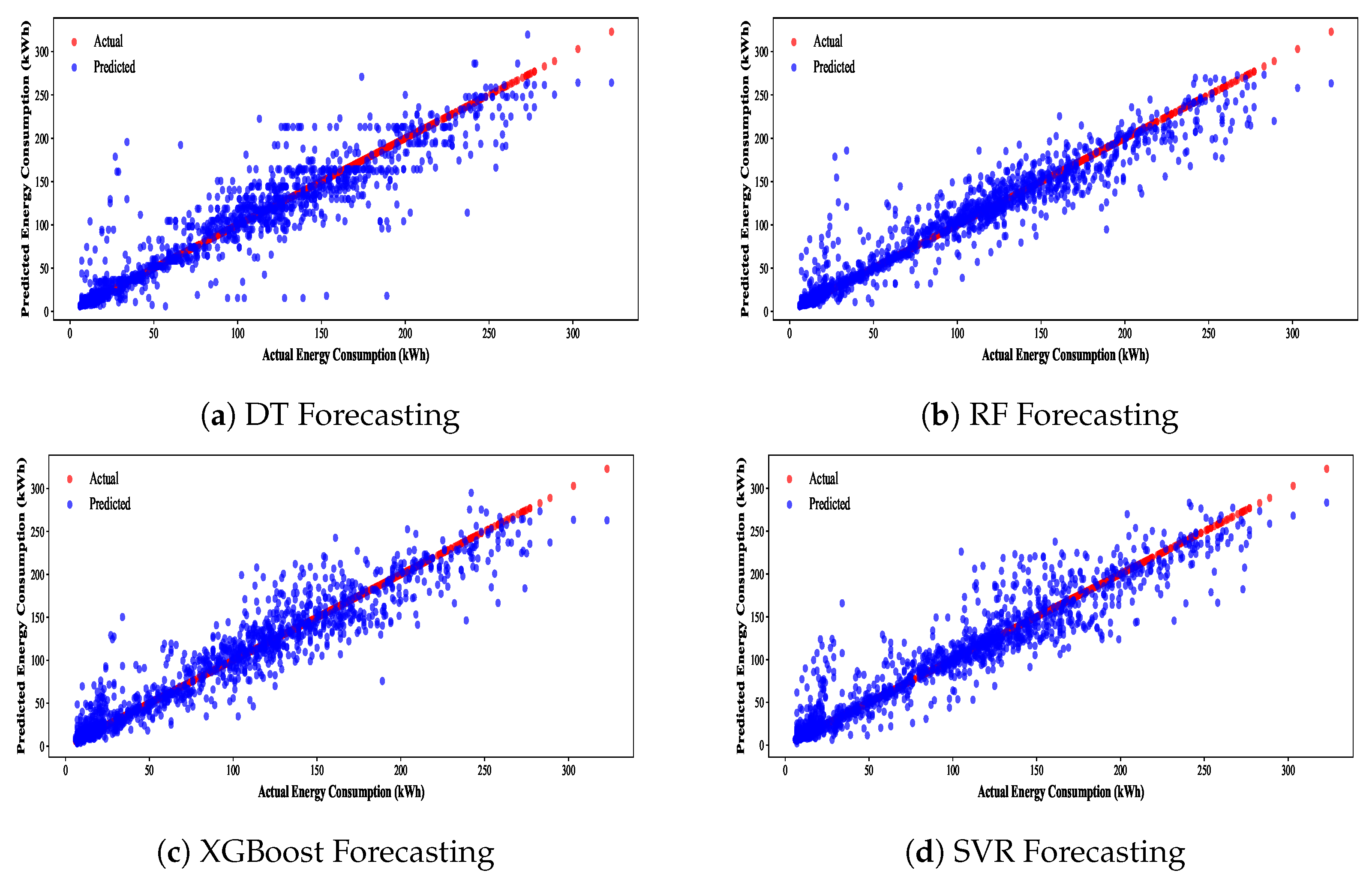
The ML models evaluated include decision tree (DT), random forest (RF), XGBoost, and support vector regression (SVR). Figure 5 compares actual power consumption with predicted values generated by these models. As summarized in Table 7, XGBoost demonstrated the highest predictive accuracy and computational efficiency, achieving the lowest MSE (i.e., 518.5), RMSE (i.e., 22.77), and higher R 2 score (i.e., 0.9010), with a training time of only 0.051 s. RF also performed competitively, offering a strong balance between accuracy and runtime, with slightly higher values of MSE, RMSE and lower R 2 score (i.e., 0.8992), and training time of 1.101 s. The DT model exhibited the fastest training time (i.e., 0.0162 s), though it exhibited slightly lower accuracy, as reflected by the R 2 score (i.e., 0.8514). In contrast, SVR showed the weakest performance, recording the highest MSE, RMSE, and the lowest R 2 score (i.e., 0.7460), with a significantly higher runtime of 41.13 s. These findings confirm that XGBoost and RF offer the most accurate and computationally efficient solutions among the evaluated ML models.
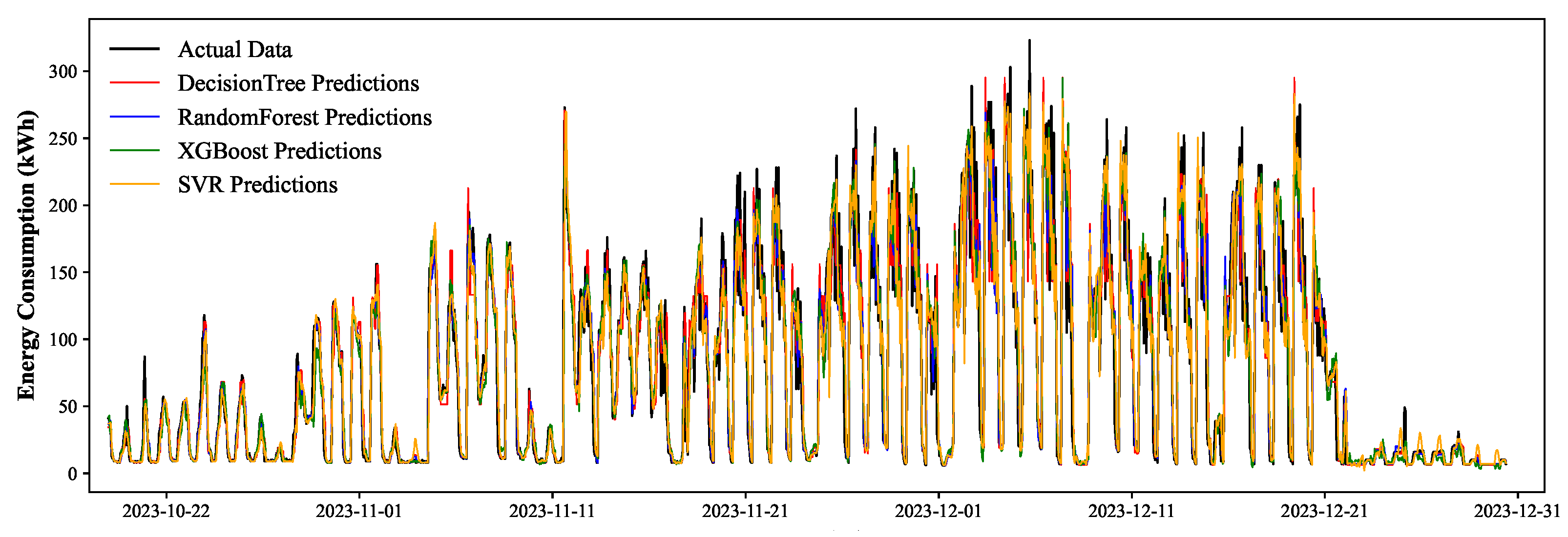
Figure 6 illustrates the comparison between actual and predicted energy consumption over the final two months of 2023. Both XGBoost and RF closely align with the actual data, accurately capturing peaks, trends, and fluctuations. The DT model shows moderate predictive ability but exhibits larger deviations from the true values. In contrast, SVR consistently underestimates energy consumption and fails to reflect sharp variations. These visual observations are consistent with the quantitative metrics discussed earlier, reinforcing the superior forecasting performance of XGBoost and RF.

4.2. Deep Learning-Based Forecasting Results

In terms of DL models, FireNet and LSTM are evaluated by assessing their ability to capture non-linear patterns and temporal dependencies in the dataset. Figure 7 presents the forecasting performance of both considered DL models. The outcomes of the comparative analysis are listed in Table 8. Compared to LSTM, FireNet achieved stronger predictive accuracy, particularly in modeling non-linear and temporal energy usage patterns. In fact, FireNet is characterized by lower MSE (i.e., 923.5 against 1280), reduced RMSE (i.e., 30.39 against 35.78), smaller MAPE (i.e., 39.90% against 96.21%), along with higher R2 (i.e., 0.8237 against 0.7558). Considering the computational time, the FireNet is faster, requiring only 22.61 s, which is less than half of the time needed by the LSTM (46.97 s). In conclusion, the FireNet model outperformed the LSTM model across all evaluated metrics, indicating enhanced precision and computational effectiveness.
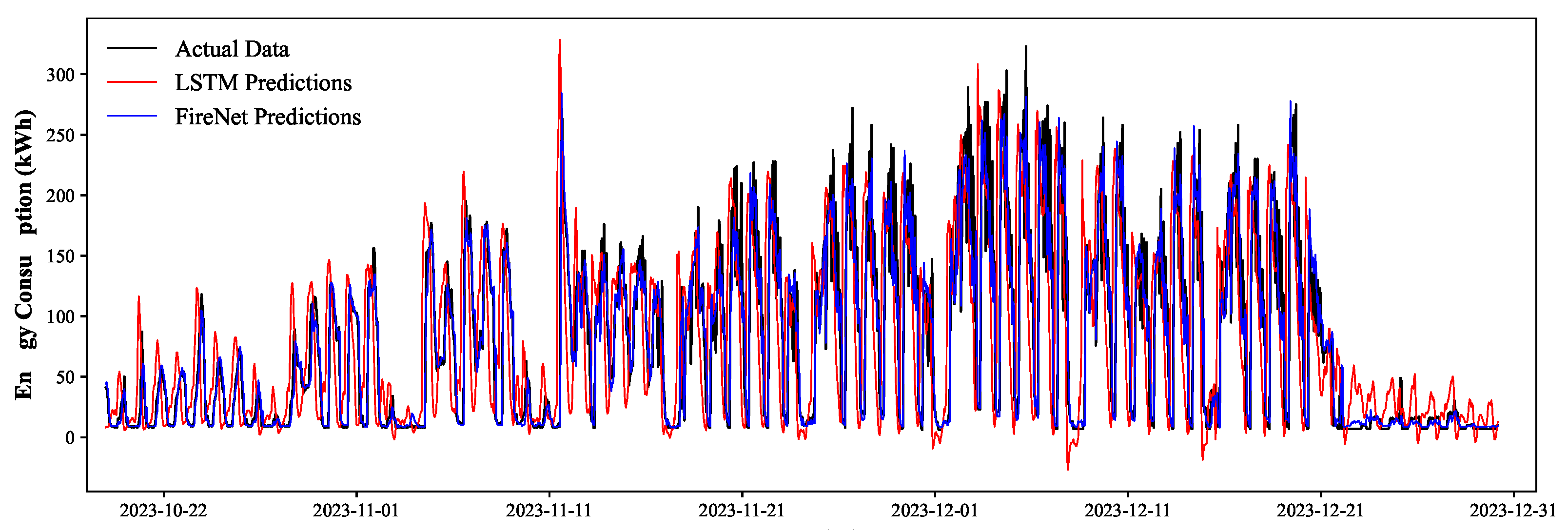
In Figure 8, the actual energy consumption is compared against the forecasts delivered by the selected DL models. As expected, FireNet’s forecasts closely align with actual values, especially during peak periods, while LSTM predictions are noticeably overestimated in case of peak demand periods.

4.3. Hybrid Model Performance

Based on the previous results, XGBoost and RF are identified as the better performing ML models, while FireNet ensures superior forecasting performance in terms of DL models. Relying on these findings, two hybrid models are developed by combining the sequential learning capabilities of FireNet with the predictive efficiency of ensemble-based ML models (i.e., XGBoost and RF). In Figure 9, the energy consumption forecasts provided by both hybrid models (i.e., FireNet–XGBoost and FireNet–RF) are shown, while the corresponding key performance parameters are reported in Table 9. The FireNet–XGBoost hybrid model demonstrated superior performance due to lower MSE (i.e., 350.2 against 418.4), reduced RMSE (i.e., 18.71 against 20.45 ), smaller MAPE (i.e., 27.00% against 29.26%), along with higher R2 (i.e., 0.9334 against 0.9205). On the other hand, the FireNet–RF hybrid model required less computation time (i.e., 21.11 s against 33.69 s). Overall, the FireNet–XGBoost model outperformed the FireNet–RF model across all evaluated metrics, indicating enhanced precision, except the computational effectiveness.
Figure 10 illustrates that the FireNet–XGBoost model closely follows actual energy consumption patterns, particularly during peak demand periods, whereas the FireNet–RF model tends to slightly overestimate energy usage across similar intervals.

5. Conclusions and Future Directions

In this paper, the effectiveness of several ML, DL, and hybrid models was tested for predicting the mid-term energy consumption in a smart commercial building. Although XGBoost was more robust than other ML techniques and FireNet managed to model non-linear relationships among the variety of DL approaches, the proposed FireNet–XGBoost hybrid demonstrated superior performance overall. This highlights the novelty of bridging the two complementary strengths of ML and DL into a general framework, and moves beyond existing studies which have traditionally relied on either approach alone.
The novelty of this study is to illustrating that a two-layer hybrid architecture can improve the accuracies and robustness with hourly horizon to offer new experiences in building energy prediction. The practical implications are considerable: more accurate load forecasts can maximize the energy consumption, minimize operational costs, and enhance the reliability of the grid, contributing to the shift to a more sustainable intelligent building operation.
The analysis was performed on data from a single smart building, which limits the generalization of the findings. The emphasis on mid-term hourly prediction also misses multi-source energy consumption data analysis or real-time dynamics. In future work, to overcome these limitations, the dataset is planned to be extended to cover multiple energy sources, to include further contextual variables, and to study real-time adaptive forecasting strategies. In addition, the community-level prediction can be extended to support cooperative energy management and demand response, as promising future work. Lastly, we will explore advanced techniques like transfer learning and attention-based architectures to improve scaling and generalization.

Author Contributions

Conceptualization, P.G. and A.H.; methodology, A.H., M.A. and M.E.; software, A.H.; validation, P.G. and M.H.; formal analysis, P.G. and G.F.; investigation, A.H.; resources, P.G., L.F. and S.M.; data curation, A.H.; writing original draft preparation, A.H. and M.A.; writing, review and editing, P.G., M.A. and A.H.; visualization, A.H.; supervision, P.G. and G.F.; funding acquisition, P.G. All authors have read and agreed to the published version of the manuscript.

Funding

This research was supported by the Piano Nazionale di Ripresa e Resilienza (PNRR) of the European Union’s NextGenerationEU program.

Conflicts of Interest

Authors Lorenzo Fenili and Silvio Messi were employed by the company ABB SACE S.p.A. The remaining authors declare that the research was conducted in the absence of any commercial or financial relationships that could be construed as a potential conflict of interest.

References

  1. Oliveira, G.M.; Vidal, D.G.; Ferraz, M.P. Urban Lifestyles and Consumption Patterns. In Encyclopedia of the UN Sustainable Development Goals; Springer: Cham, Switzerland, 2020; pp. 851–860. [Google Scholar] [CrossRef]
  2. Bilgen, S. Structure and environmental impact of global energy consumption. Renew. Sustain. Energy Rev. 2014, 38, 890–902. [Google Scholar] [CrossRef]
  3. González-Torres, M.; Pérez-Lombard, L.; Coronel, J.F.; Maestre, I.R.; Yan, D. A review on buildings energy information: Trends, end-uses, fuels and drivers. Energy Rep. 2022, 8, 626–637. [Google Scholar] [CrossRef]
  4. Afshan, S.; Ozturk, I.; Yaqoob, T. Facilitating renewable energy transition, ecological innovations and stringent environmental policies to improve ecological sustainability. Renew. Energy 2022, 196, 151–160. [Google Scholar] [CrossRef]
  5. Salkuti, S.R. Emerging and Advanced Green Energy Technologies for Sustainable and Resilient Future Grid. Energies 2022, 15, 6667. [Google Scholar] [CrossRef]
  6. Zhao, J.; Patwary, A.K.; Qayyum, A.; Alharthi, M.; Bashir, F.; Mohsin, M.; Hanif, I.; Abbas, Q. The determinants of renewable energy sources for the fueling of green and sustainable economy. Energy 2022, 238, 122029. [Google Scholar] [CrossRef]
  7. Giovanni, G.D.; Rotilio, M.; Giusti, L.; Ehtsham, M. Exploiting building information modeling and machine learning for optimizing rooftop photovoltaic systems. Energy Build. 2024, 313, 114250. [Google Scholar] [CrossRef]
  8. Ehtsham, M.; Rotilio, M.; Cucchiella, F. Deep learning augmented medium-term photovoltaic energy forecasting. Energy Rep. 2025, 13, 4299–4317. [Google Scholar] [CrossRef]
  9. El-Afifi, M.I.; Sedhom, B.E.; Eladl, A.A.; Elgamal, M.; Siano, P. Demand side management strategy for smart building using multi-objective hybrid optimization technique. Results Eng. 2024, 22, 102265. [Google Scholar] [CrossRef]
  10. Raza, A.; Jingzhao, L.; Adnan, M.; Ahmad, I. Optimal load forecasting and scheduling strategies for smart homes peer-to-peer energy networks. Results Eng. 2024, 22, 102188. [Google Scholar] [CrossRef]
  11. Ehtsham, M.; Rotilio, M.; Cucchiella, F.; Giovanni, G.D.; Schettini, D. Investigating the effects of hyperparameter sensitivity on machine learning algorithms for PV forecasting. In Proceedings of the E3S Web of Conferences; EDP Sciences: Les Ulis, France, 2025; Volume 612, p. 01002. [Google Scholar] [CrossRef]
  12. Lazos, D.; Sproul, A.B.; Kay, M. Optimisation of energy management in commercial buildings with weather forecasting inputs: A review. Renew. Sustain. Energy Rev. 2014, 39, 587–603. [Google Scholar] [CrossRef]
  13. Iqbal, N.; Kim, D.H. IoT task management mechanism based on predictive optimization for efficient energy consumption in smart residential buildings. Energy Build. 2022, 257, 111762. [Google Scholar] [CrossRef]
  14. Pawar, P.; TarunKumar, M. An IoT based Intelligent Smart Energy Management System. Measurement 2020, 152, 107187. [Google Scholar] [CrossRef]
  15. Khan, S.U.; Khan, N.; Ullah, F.U.M.; Kim, M.J.; Lee, M.Y.; Baik, S.W. Towards intelligent building energy management: AI-based framework for power consumption and generation forecasting. Energy Build. 2023, 279, 112705. [Google Scholar] [CrossRef]
  16. Mathumitha, R.; Rathika, P.; Manimala, K. Intelligent deep learning techniques for energy consumption forecasting in smart buildings: A review. Artif. Intell. Rev. 2024, 57, 35. [Google Scholar] [CrossRef]
  17. Santos, M.L.; García, S.D.; García-Santiago, X.; Ogando-Martínez, A.; Camarero, F.E.; Gil, G.B.; Ortega, P.C. Deep learning and transfer learning techniques applied to short-term load forecasting of data-poor buildings in local energy communities. Energy Build. 2023, 292, 113164. [Google Scholar] [CrossRef]
  18. Wahid, F.; Ghazali, R.; Shah, A.S.; Fayaz, M. Prediction of energy consumption in the buildings using multi-layer perceptron and random forest. Int. J. Adv. Sci. Technol. 2017, 101, 13–22. [Google Scholar] [CrossRef]
  19. NASA Power Data Access Viewer: Prediction of Worldwide Energy Resource. Available online: https://power.larc.nasa.gov/data-access-viewer/ (accessed on 1 February 2025).
  20. International Energy Agency. World Energy Outlook 2024; IEA: Paris, France, 2024. [Google Scholar]
  21. Wang, Z.; Wang, Y.; Zeng, R.; Srinivasan, R.S.; Ahrentzen, S. Random Forest based hourly building energy prediction. Energy Build. 2018, 171, 11–25. [Google Scholar] [CrossRef]
  22. Chou, J.S.; Tran, D.S. Forecasting energy consumption time series using machine learning techniques based on usage patterns of residential householders. Energy 2018, 165, 709–726. [Google Scholar] [CrossRef]
  23. Amasyali, K.; El-Gohary, N.M. A review of data-driven building energy consumption prediction studies. Renew. Sustain. Energy Rev. 2018, 81, 1192–1205. [Google Scholar] [CrossRef]
  24. Wang, J.Q.; Du, Y.; Wang, J. LSTM based long-term energy consumption prediction with periodicity. Energy 2020, 197, 117197. [Google Scholar] [CrossRef]
  25. Alam, G.M.I.; Tasnia, N.; Biswas, T.; Hossen, M.J.; Tanim, S.A.; Miah, M.S.U. Real-Time Detection of Forest Fires Using FireNet-CNN and Explainable AI Techniques. IEEE Access 2025, 13, 51150–51181. [Google Scholar] [CrossRef]
  26. Yesilyurt, H.; Dokuz, Y.; Dokuz, A.S. Data-driven energy consumption prediction of a university office building using machine learning algorithms. Energy 2024, 310, 133242. [Google Scholar] [CrossRef]
  27. Alotaibi, B.S.; Abuhussain, M.A.; Dodo, Y.A.; Al-Tamimi, N.; Maghrabi, A.; Ojobo, H.; Naibi, A.U.; Benti, N.E. A novel approach to estimate building electric power consumption based on machine learning method: Toward net-zero energy, low carbon and smart buildings. Int. J. Low-Carbon Technol. 2024, 19, 2335–2345. [Google Scholar] [CrossRef]
  28. Gao, Z.; Yu, J.; Zhao, A.; Hu, Q.; Yang, S. A hybrid method of cooling load forecasting for large commercial building based on extreme learning machine. Energy 2022, 238, 122073. [Google Scholar] [CrossRef]
  29. Kim, T.Y.; Cho, S.B. Predicting residential energy consumption using CNN-LSTM neural networks. Energy 2019, 182, 72–81. [Google Scholar] [CrossRef]
  30. Olu-Ajayi, R.; Alaka, H.; Sulaimon, I.; Sunmola, F.; Ajayi, S. Building energy consumption prediction for residential buildings using deep learning and other machine learning techniques. J. Build. Eng. 2022, 45, 103406. [Google Scholar] [CrossRef]
  31. Sunder, R.; R, S.; Paul, V.; Punia, S.K.; Konduri, B.; Nabilal, K.V.; Lilhore, U.K.; Lohani, T.K.; Ghith, E.; Tlija, M. An advanced hybrid deep learning model for accurate energy load prediction in smart building. Energy Explor. Exploit. 2024, 42, 2241–2269. [Google Scholar] [CrossRef]
  32. Yenagimath, M. Electrical Load Forecasting using Improved Feature Selection and Hybrid Deep Learning Algorithms for Power System Situational Awareness. Deleted J. 2024, 20, 2825–2836. [Google Scholar] [CrossRef]
  33. Lu, H.; Wu, J.; Ruan, Y.; Qian, F.; Meng, H.; Gao, Y.; Xu, T. A multi-source transfer learning model based on LSTM and domain adaptation for building energy prediction. Int. J. Electr. Power Energy Syst. 2023, 149, 109024. [Google Scholar] [CrossRef]
  34. Peng, X.; Li, Y.; Zhou, H. Transfer Learning and Attention-Enhanced Seq2Seq Model for Green Building Load Forecasting. Sci. Rep. 2025, 15, 16953. [Google Scholar] [CrossRef] [PubMed]
  35. Chen, G.; Lu, S.; Zhou, S.; Tian, Z.; Kim, M.; Liu, J.; Liu, X. A Systematic Review of Building Energy Consumption Prediction: From Perspectives of Load Classification, Data-Driven Frameworks, and Future Directions. Appl. Sci. 2025, 15, 3086. [Google Scholar] [CrossRef]
  36. Zhong, H.; Wang, J.; Jia, H.; Mu, Y.; Lv, S. Vector field-based support vector regression for building energy consumption prediction. Appl. Energy 2019, 242, 403–414. [Google Scholar] [CrossRef]
  37. Lahouar, A.; Slama, J.B.H. Day-ahead load forecast using random forest and expert input selection. Energy Convers. Manag. 2015, 103, 1040–1051. [Google Scholar] [CrossRef]
  38. Cao, L.; Li, Y.; Zhang, J.; Jiang, Y.; Han, Y.; Wei, J. Electrical load prediction of healthcare buildings through single and ensemble learning. Energy Rep. 2020, 6, 2751–2767. [Google Scholar] [CrossRef]
  39. Ismail, L.; Materwala, H.; Dankar, F.K. Machine Learning Data-Driven Residential Load Multi-Level Forecasting with Univariate and Multivariate Time Series Models Toward Sustainable Smart Homes. IEEE Access 2024, 12, 55632–55668. [Google Scholar] [CrossRef]
  40. Somu, N.; R, G.R.M.; Ramamritham, K. A deep learning framework for building energy consumption forecast. Renew. Sustain. Energy Rev. 2021, 137, 110591. [Google Scholar] [CrossRef]
  41. Hussain, A.; Franchini, G.; Giangrande, P.; Mandelli, G.; Fenili, L. A Comparative Analysis of Machine Learning Models for Medium-Term Load Forecasting in Smart Commercial Building. In Proceedings of the 2024 IEEE 12th International Conference on Smart Energy Grid Engineering (SEGE), Oshawa, ON, Canada, 18–20 August 2024; pp. 228–232. [Google Scholar] [CrossRef]
  42. Chandler, W.S.; Hoell, J.M.; Westberg, D.; Zhang, T.; Stackhouse, P.W. NASA Prediction of Worldwide Energy Resource High Resolution Meteorology Data For Sustainable Building Design; Technical Report; NASA: Washington, DC, USA, 2013. [Google Scholar]
  43. Zhang, J.; Xu, Z.; Wei, Z. Absolute Logarithmic Calibration for Correlation Coefficient with Multiplicative Distortion. Commun. Stat.-Simul. Comput. 2023, 52, 482–505. [Google Scholar] [CrossRef]
  44. Breiman, L. Random forests. Mach. Learn. 2001, 45, 5–32. [Google Scholar] [CrossRef]
  45. Mallala, B.; Azeez Khan, P.; Pattepu, B.; Eega, P.R. Integrated Energy Management and Load Forecasting Using Machine Learning. In Proceedings of the 2024 2nd International Conference on Sustainable Computing and Smart Systems (ICSCSS), Coimbatore, India, 10–12 July 2024; pp. 1004–1009. [Google Scholar] [CrossRef]
  46. Zhu, J.; Dong, H.; Zheng, W.; Li, S.; Huang, Y.; Xi, L. Review and prospect of data-driven techniques for load forecasting in integrated energy systems. Appl. Energy 2022, 321, 119269. [Google Scholar] [CrossRef]
  47. Xie, Z.; Wang, R.; Wu, Z.; Liu, T. Short-Term Power Load Forecasting Model Based on Fuzzy Neural Network using Improved Decision Tree. In Proceedings of the 2019 IEEE Sustainable Power and Energy Conference (iSPEC), Beijing, China, 21–23 November 2019; pp. 482–486. [Google Scholar] [CrossRef]
  48. Alrobaie, A.; Krarti, M. A Review of Data-Driven Approaches for Measurement and Verification Analysis of Building Energy Retrofits. Energies 2022, 15, 7824. [Google Scholar] [CrossRef]
  49. Olawuyi, A.; Ajewole, T.; Oladepo, O.; Awofolaju, T.T.; Agboola, M.; Hasan, K. Development of an Optimized Support Vector Regression Model Using Hyper-Parameters Optimization for Electrical Load Prediction. UNIOSUN J. Eng. Environ. Sci. 2024, 6. [Google Scholar] [CrossRef]
  50. Friedman, J.H. Greedy Function Approximation: A Gradient Boosting Machine. Ann. Stat. 2001, 29, 1189–1232. [Google Scholar] [CrossRef]
  51. Lazzari, F.; Mor, G.; Cipriano, J.; Gabaldon, E.; Grillone, B.; Chemisana, D.; Solsona, F. User behavior models to forecast electricity consumption of residential customers based on smart metering data. Energy Rep. 2022, 8, 3680–3691. [Google Scholar] [CrossRef]
  52. Dabrowski, J.J.; Zhang, Y.; Rahman, A. ForecastNet: A Time-Variant Deep Feed-Forward Neural Network Architecture for Multi-step-Ahead Time-Series Forecasting. In Neural Information Processing. ICONIP 2020; Yang, H., Pasupa, K., Leung, A.C.S., Kwok, J.T., Chan, J.H., King, I., Eds.; Lecture Notes in Computer Science; Springer: Cham, Switzerland, 2020; Volume 12534. [Google Scholar] [CrossRef]
  53. Forootan, M.M.; Larki, I.; Zahedi, R.; Ahmadi, A. Machine Learning and Deep Learning in Energy Systems: A Review. Sustainability 2022, 14, 4832. [Google Scholar] [CrossRef]
  54. Rafi, S.H.; Nahid-Al-Masood; Deeba, S.R.; Hossain, E. A Short-Term Load Forecasting Method Using Integrated CNN and LSTM Network. IEEE Access 2021, 9, 32436–32448. [Google Scholar] [CrossRef]
  55. Hussain, A.; Giangrande, P.; Franchini, G.; Fenili, L.; Messi, S. Analyzing the Effect of Error Estimation on Random Missing Data Patterns in Mid-Term Electrical Forecasting. Electronics 2025, 14, 1383. [Google Scholar] [CrossRef]
  56. Hakyemez, T.C.; Adar, O. Testing the Efficacy of Hyperparameter Optimization Algorithms in Short-Term Load Forecasting. arXiv 2024, arXiv:2410.15047. [Google Scholar] [CrossRef]
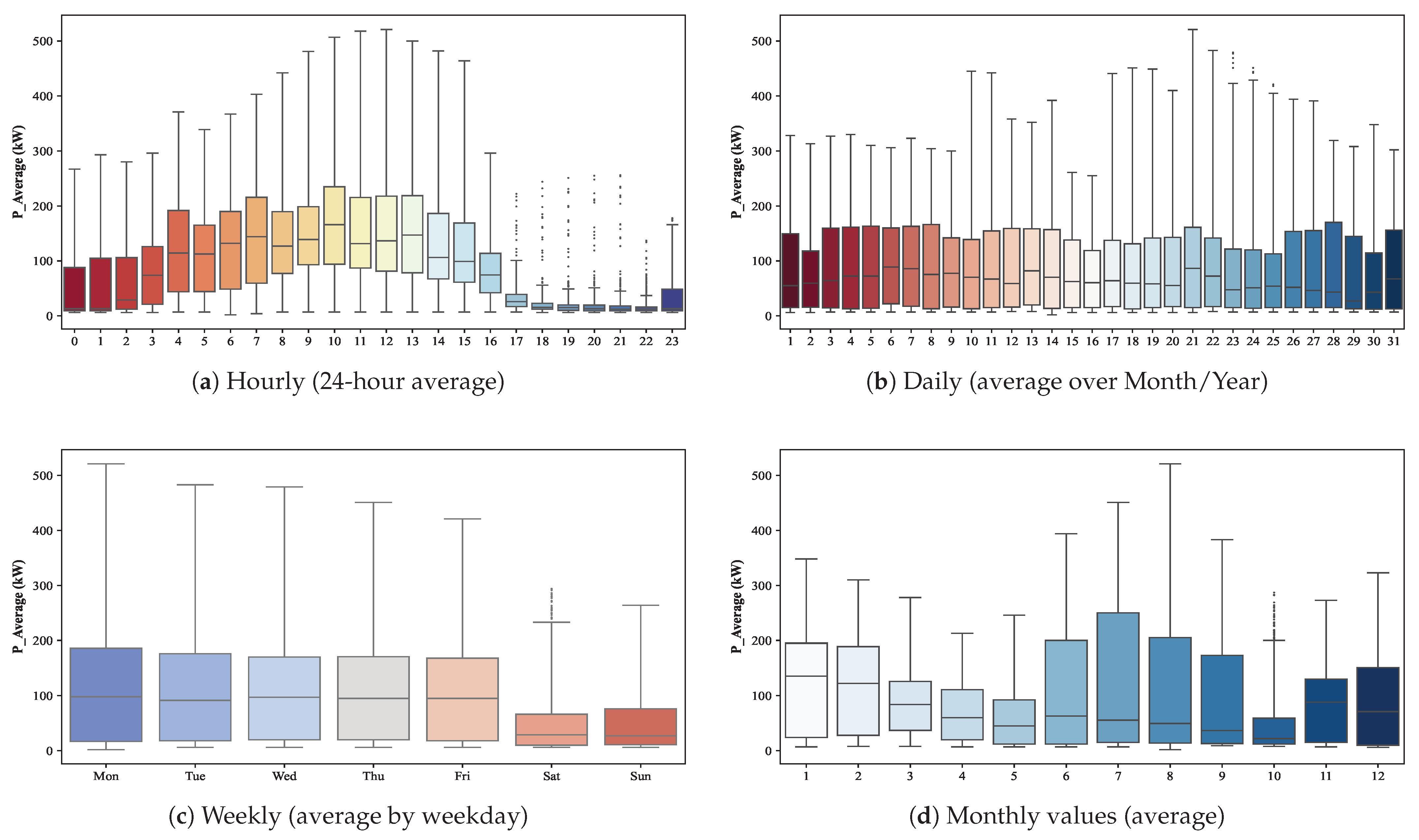
Figure 1. Time-based profiling of active power: (a) Hourly, (b) Daily, (c) Weekly, and (d) Monthly values.
Applsci 15 10066 g001
Figure 2. Comparison of power consumption trends at different time scales.
Applsci 15 10066 g002
Figure 3. Proposed methodology workflow for energy consumption forecasting.
Applsci 15 10066 g003
Figure 4. Pearson correlation among energy and meteorological features.
Applsci 15 10066 g004
Figure 5. Forecasting performance of ML models. (a) DT. (b) RF. (c) XGBoost. (d) SVR.
Applsci 15 10066 g005
Figure 6. Actual vs. predicted energy consumption for ML models.
Applsci 15 10066 g006
Figure 7. Forecasting performance using DL models. (a) FireNet. (b) LSTM.
Applsci 15 10066 g007
Figure 8. Actual vs. predicted energy consumption for DL models.
Applsci 15 10066 g008
Figure 9. Forecasting performance using hybrid models. (a) FireNet–XGBoost. (b) FireNet–RF.
Applsci 15 10066 g009
Figure 10. Actual vs. predicted energy consumption for hybrid models.
Applsci 15 10066 g010
Table 2. Sample records of linear power consumption parameters.
DateTime P Avg
(kW)
P Min
(kW)
P Max
(kW)
Q Avg
(kvar)
Q Min
(kvar)
Q Max
(kvar)
S Avg
(kVA)
S Min
(kVA)
S Max
(kVA)
1 January 202108:00:00356336376322936311291331
1 January 202109:00:00345324373302633300279328
1 January 202110:00:00351329380312837306284336
1 January 202111:00:00357334387332937312289343
1 January 202112:00:00361331389332836316287345
Table 3. Sample records of non-linear weather data parameters.
DateTimeGb(i)
(W/m2)
Gd(i)
(W/m2)
H_sun
(h)
T2m
(°C)
WS10m
(m/s)
1 January 202108:00:0056.00543.8008.39−1.4401.585
1 January 202109:00:00103.13975.93314.831.1000.997
1 January 202110:00:00142.20696.40019.253.8660.483
1 January 202111:00:00186.00793.73321.204.9330.593
1 January 202111:00:00165.27397.20020.495.1430.745
Table 4. Electrical load classification according to the index.
IndexElectrical Load Classification
1Original time-series data (unmodified raw observations).
2Weekdays (Monday to Friday), excluding Holidays.
3Weekend (Saturday and Sunday) and Holidays.
4Statistical aggregation features: Daily, Weekly, and Monthly Averages.
5Seasonal categorization into Winter, Spring, Summer, and Autumn.
Table 5. FireNet architecture for energy forecasting.
BlockFiltersKernel SizePool SizeOutput Shape
13252 ( T / 2 , 32 )
26452 ( T / 4 , 64 )
312832 ( T / 8 , 128 )
425632 ( T / 16 , 256 )
55123 ( T / 16 , 512 )
Table 6. Hyper-parameter tuning of different models.
ModelParameterRangeOptuna Value
Decision Treemax_depth[10, 20, 30, 50, 100]7
min_samples_split[2, 3, 5, 10]10
min_samples_leaf[1, 5, 10]8
criterion[mse, mae]mse
split_strategy[best, random]best
Random Forestn_estimators[50, 100, 150, 200, 300]80
max_depth[10, 30, 50, 70, 100, None]13
min_samples_split[2, 3, 5, 10]7
min_samples_leaf[1, 2, 3, 4, 5]5
max_features[auto, sqrt, log2]sqrt
bootstrap[True, False]True
XGBoostn_estimators[50, 300]261
max_depth[3, 20]4
learning_rate[0.01, 0.3]0.051
subsample[0.5, 1.0]0.949
colsample_bytree[0.5, 1.0]0.813
gamma[0, 5]3.704
reg_alpha[0, 5]3.083
reg_lambda[0, 5]3.442
SVRC[0.1, 100] (log)34.95
epsilon[0.001, 1.0] (log)0.244
kernel[rbf, linear]rbf
gamma[scale, auto]auto
FireNetfilters[32, 64, 128]64
dropout_rate[0.2, 0.5] (uniform)0.2132
learning_rate[0.0005, 0.01] (log)0.000507
batch_size[16, 32, 64]64
LSTMunits[32, 50, 64]32
dropout_rate[0.1, 0.5] (uniform)0.285
learning_rate[0.0005, 0.01] (log)0.007215
batch_size[16, 32, 64]16
Table 7. Forecasting performance metrics of ML models.
ModelTraining Time (s)MSERMSER2 ScoreMAPE (%)
DT0.01620778.227.900.851435.68
RF1.101527.722.970.899233.63
XGBoost0.05100518.522.770.901037.17
SVR41.13211145.950.746044.79
Table 8. Forecasting performance of DL models based on standard metrics.
ModelTraining Time (s)MSERMSER2 ScoreMAPE (%)
FireNet22.61923.530.390.823739.90
LSTM46.97128035.780.755896.21
Table 9. Forecasting performance of hybrid ML and DL models.
ModelTraining Time (s)MSERMSER2MAPE (%)
FireNet-XGBoost33.69350.218.710.933427.00
FireNet-RF21.11418.420.450.920529.26
Disclaimer/Publisher’s Note: The statements, opinions and data contained in all publications are solely those of the individual author(s) and contributor(s) and not of MDPI and/or the editor(s). MDPI and/or the editor(s) disclaim responsibility for any injury to people or property resulting from any ideas, methods, instructions or products referred to in the content.