Incorporating Transverse Normal Strain in the Homogenization of Corrugated Cardboards

Abstract

Homogenization researches for corrugated cardboard are predominantly based on plate theories assuming constant thickness, such as the Reissner–Mindlin plate. However, corrugated cardboard is prone to significant deformation in the thickness direction. To address this limitation, the present work proposes an improved plate element designed by expanding the deflection function to the quadratic term of the thickness coordinate, enabling a linearly varied transverse normal strain. Furthermore, an extension of the established homogenization method is developed to derive the constitutive matrix. The element is implemented via the Abaqus user subroutine UEL. Validation demonstrates that the proposed element effectively characterizes a linearly varied transverse normal strain and stress. Simulation results from the homogenized model applying the proposed element and extended homogenization method are compared with those from detailed models. The comparisons confirm the efficiency and accuracy of the proposed approach.

1. Introduction

Corrugated cardboard exhibits the advantages of a high strength-to-weight ratio, being environmentally sustainable, and economical, leading to a widespread use in the packaging sector. It is a sandwich structure composed of several layers of flat papers (called liners or facing), and wave-shaped corrugated paper (called flutes or core), bonded together with adhesive. The load-bearing mechanism of corrugated cardboard is analogous to an I-beam. The liners are separated by the flutes, increasing the cross-sectional moment of inertia and thereby enhancing the flexural stiffness, while the flutes resist the transverse shear. Consequently, liners utilize higher-performance paper with superior pulp quality and greater grammage compared to the flutes.

According to the composition of liners and flutes, corrugated cardboard can be categorized as single-face, single-wall, double-wall, triple-wall, etc. Key parameters characterizing a flute are its height, period, and corrugation factor. The corrugation factor (also known as take-up factor or wave number) is defined as the length ratio of a flute to a liner. Common parameter sets are classified into distinct flute types as summarized in

Table 1. Parameters of common flute types.

Flute Type	Height (mm)	Period (mm)	Corrugation Factor
A	4.8	8.0–9.5	$\approx$1.50
B	3.2	5.5–6.5	$\approx$1.40
C	4.0	6.8–7.9	$\approx$1.45
E	1.6	3.0–3.5	$\approx$1.25
F	0.8	1.9–2.6	$\approx$1.25

.

Paper sheet and corrugated cardboard are both orthotropic material with three principal directions: machine direction (MD), cross direction (CD), and thickness direction (ZD). For paper sheet, MD is the direction that paper comes out of the papermaking machine, CD lies perpendicular to MD within the sheet plane, and ZD is normal to the sheet surface. For corrugated cardboard, MD is perpendicular to the corrugation profile, while CD is parallel to it, as shown in Figure 1. MD exhibits higher fiber alignment, resulting in better mechanical performance than CD for both paper sheet and corrugated cardboard.

When modeling corrugated cardboard in FEA, a trade-off exists between geometry complexity and computational efficiency. It is difficult and tedious to model every flute and liner. Although it might help to capture local deformations, it incurs prohibitive computational costs, particularly for large-scale problems. Therefore, characterizing mechanical properties at the macroscale and homogenizing the cardboard into an equivalent orthotropic plate is preferable.

Analytical methods for corrugated cardboard homogenization are broadly classified into two categories. The first employs structural mechanics frameworks to derive equivalent properties. Early work by Briassoulis [1] provided analytical expressions using beam theory under Kirchhoff plate theory. Biancolini [2] extended this methodology to sinusoidal corrugated cardboard. Nordstrand [3] derived the transverse shear stiffness for diverse corrugation shapes via curved beam theory. Bartolozzi [4] applied an energetic approach to compute equivalent properties under Reissner–Mindlin plate theory. Abbès [5] decomposed the torsional problem of orthotropic cardboard into the torsion of two orthogonal beams to obtain the equivalent torsional stiffness.

The second category utilizes laminated plate theory with coordinate transformation, which was originally developed for fiber orientation in composites, adapted to corrugated structure with modified rotation axes. Aboura [6] established fundamental procedures for this method under the framework of classical laminated plate theory (CLPT), later refined by Talbi [7] to first-order shear deformation theory (FSDT) with corrections. Minh [8] further extended it to double-wall corrugated cardboard. This approach is accepted by many researchers [9,10] due to its simplicity.

In addition to analytical methods, there are numerical [11] and experimental [12] methods of corrugated cardboard homogenization.

Although FSDT improves upon CPT by incorporating transverse shear effects, both theories still assume thickness incompressibility. Consequently, these homogenization schemes are suitable for scenarios with negligible through-thickness deformation (i.e., transverse normal strain), such as the box compression test, where the load is primarily borne by the side panels and peak load is governed by panel buckling.

However, we cannot overlook the fact that corrugated cardboard is prone to significant through-thickness deformation, which enables cushioning usage. Extensive research exists on its out-of-plane properties: Krusper [13] conducted nonlinear analyses on the out-of-plane compression; Huang [14] investigated vibration stiffness and damping; and Wang [15] studied energy absorption under varying humidity. Nevertheless, most studies on transverse normal strain remain stand-alone efforts, being incompatible with the aforementioned homogenization approaches.

There are scenarios wherein it is necessary to incorporate transverse normal strain into the homogenized plate model, yet related studies remain scarce. For instance, in a carton fully filled with products, vertical loading may induce significant through-thickness deformation in flaps, rendering plate elements insufficient. Similarly, in simulations of carton drop tests or tip-over tests, various criteria dictate that the box may impact the floor with its face, edge, or corner. In such cases, all deformation components must be considered to prevent biased results. In fact, the mechanism of drop test is so complex that it is still a tricky problem in industry. Beyond packaging, corrugated cardboard finds applications in numerous scenarios such as sustainable furniture. It is valuable to pursue a general solution that can be applied to diverse situations. Therefore, the established homogenization method using laminated plate theory is extended in the present work.

It should be noted that a common misconception may arise: capturing through-thickness deformation cannot be achieved merely by switching from shell elements to solid or solid-shell elements. Indeed, elements such as SC8R and CSS8 in Abaqus (2022) [16], SOLSH190 in ANSYS (2024 R2) [17], are capable of characterizing the transverse normal strain. These elements have the same topology and degrees of freedom (DOFs) as solid elements and are developed by applying the displacement constraints of shell theory to enable a good performance on a thin-walled structure problem as well as transverse normal strain [18,19].

However, the corrugated structure is not a homogeneous material but one with cavities, which is both materially and structurally orthotropic. The sectional moment of inertia on MD and CD are inherently unequal, while a topology of a solid element implies an equality. As Biancolinni [11] notes: “due to the corrugated structure, the core cannot be reduced to an equivalent orthotropic material valid for both bending and stretching”. Consequently, corrugated cardboard should be homogenized with plate elements because it is a 2D plane abstracted from a 3D solid, and the discrepancy between in-plane and flexural stiffnesses can be solved by specifying the constitutive matrix directly.

Two features provided by Abaqus can be used to specify the constitutive matrix: General Shell Stiffness section [20] and user subroutine UGENS [21]. However, these can only be applied on a conventional shell (planar element), which is rooted in FSDT [16]. To overcome this limitation, a custom element is required.

From a theoretical perspective, incorporating transverse normal strain necessitates manipulating the displacement functions u, v and w to include high order terms of the thickness coordinate, which can be broadly concluded as parts of high-order shear deformation theory (HSDT). Carrera [22] developed a unified framework enabling displacement expansions to any order. While higher-order expansions generally improve accuracy, they also introduce additional unknown functions that complicate the formulation. In the present work, transverse normal strain is the primary focus, while transverse shear is regarded as adequate for FSDT. Consequently, we adopt a formulation that expands the deflection function w to the second order to introduce linearly varied transverse normal strain while maintaining the FSDT framework for transverse shear.

Regarding finite element implementation, high-order theories demand greater shape function continuity with schemes of special shape function [23]; or alternatively a penalty approach can be applied [24]. Otherwise, the number of DOFs increases. In a household program it is not a problem to increase DOFs, but this work aims for compatibility with commercial software workflows. Therefore, the element is implemented via an Abaqus (2022) user subroutine UEL. The extra DOFs can be settled using established techniques from the literature [25,26,27], which effectively repurpose existing DOFs.

2. Plate Element Incorporating Transverse Normal Strain

2.1. Theory

The transverse normal strain in FSDT is zero because the deflection function w is independent of the thickness coordinate z. Therefore, by expanding the deflection function to the higher-order terms of z, the transverse normal strain can be introduced. According to Carrera’s unified formulation [22], the displacement field can be expanded to any order of the thickness coordinate. For the simplicity of the model and the convergence of the element, it is more appropriate to expand to the second order so that the transverse normal strain is distributed linearly. The displacement field is assumed to be:

$$\begin{array}{l}u=u_0(x,y)+z{\phi }_y(x,y)\\ v=v_0(x,y)-z{\phi }_x(x,y)\\ w=w_0(x,y)+z\psi (x,y)+z^2\zeta (x,y)\end{array}$$

(1)

where $u_0$, $v_0$ and $w_0$ are displacement components of the middle surface, ${\phi }_x$ and ${\phi }_y$ are rotation angles of x-axis and y-axis, and ψ and ζ are the extra unknown functions. Together, there are seven unknown functions in Equation (1) to be determined, i.e., seven degrees of freedom.

Based on the displacement field, a systematic process can be applied to derive the kinematic, constitutive, and equilibrium equations—refer to references [28,29]. The detailed derivations can be seen in Appendix A. Only the constitutive matrix, which will be calculated in Section 3, is listed here.

$$\left\{\begin{array}{c}{N}_x\\ N_y\\ N_{xy}\\ N_z\\ Q_{xz}\\ Q_{yz}\\ M_x\\ M_y\\ M_{xy}\\ M_z\\ R_{xz}\\ R_{yz}\\ S_{xz}\\ S_{yz}\end{array}\right\}=\left[\begin{array}{cccccccccccccc}{A}_{11}& A_{12}& 0& A_{13}& 0& 0& B_{11}& B_{12}& 0& B_{13}& 0& 0& 0& 0\\ & A_{22}& 0& A_{23}& 0& 0& B_{21}& B_{22}& 0& B_{23}& 0& 0& 0& 0\\ & & A_{44}& 0& 0& 0& 0& 0& B_{44}& 0& 0& 0& 0& 0\\ ⋮& & \ddots & A_{33}& 0& 0& B_{31}& B_{32}& 0& B_{33}& 0& 0& 0& 0\\ & & & & A_{55}& 0& 0& 0& 0& 0& B_{55}& 0& C_{55}& 0\\ & & & & & A_{66}& 0& 0& 0& 0& 0& B_{66}& 0& C_{66}\\ & & & & & & C_{11}& C_{12}& 0& C_{13}& 0& 0& 0& 0\\ & & & & & & & C_{22}& 0& C_{23}& 0& 0& 0& 0\\ & & & & & & & & C_{44}& 0& 0& 0& 0& 0\\ ⋮& & & & & & & & \ddots & C_{33}& 0& 0& 0& 0\\ & & & & & & & & & & C_{55}& 0& D_{55}& 0\\ & & & & & & & & & & & C_{66}& 0& D_{66}\\ & & & & & & & & & & & & E_{55}& 0\\ & & \dots & & & & & & \dots & & & & & E_{66}\end{array}\right]·\left\{\begin{array}{c}{\epsilon }_x^0\\ {\epsilon }_y^0\\ {\gamma }_{xy}^0\\ {\epsilon }_z^0\\ {\gamma }_{xz}^0\\ {\gamma }_{yz}^0\\ {\kappa }_x\\ {\kappa }_y\\ {\kappa }_{xy}\\ {\kappa }_z\\ {\kappa }_{xz}\\ {\kappa }_{yz}\\ {\theta }_{xz}\\ {\theta }_{yz}\end{array}\right\}$$

(2)

with

$$\left[\begin{array}{ccccc}A& B& C& D& E\end{array}\right]={\displaystyle {\int }_{-h/2}^{h/2}Q}\left(\begin{array}{ccccc}1& z& z^2& z^3& z^4\end{array}\right)dz$$

(3)

where Q is the elastic matrix of orthotropic material as follows:

$$\left\{\begin{array}{c}{\sigma }_x\\ {\sigma }_y\\ {\tau }_{xy}\\ {\sigma }_z\\ {\tau }_{xz}\\ {\tau }_{yz}\end{array}\right\}=\left[\begin{array}{cccccc}{Q}_{11}& Q_{12}& & Q_{13}& & \\ Q_{21}& Q_{22}& & Q_{23}& & \\ & & Q_{44}& & & \\ Q_{31}& Q_{32}& & Q_{33}& & \\ & & & & Q_{55}& \\ & & & & & Q_{66}\end{array}\right]\cdot \left\{\begin{array}{c}{\epsilon }_x\\ {\epsilon }_y\\ {\gamma }_{xy}\\ {\epsilon }_z\\ {\gamma }_{xz}\\ {\gamma }_{yz}\end{array}\right\}$$

(4)

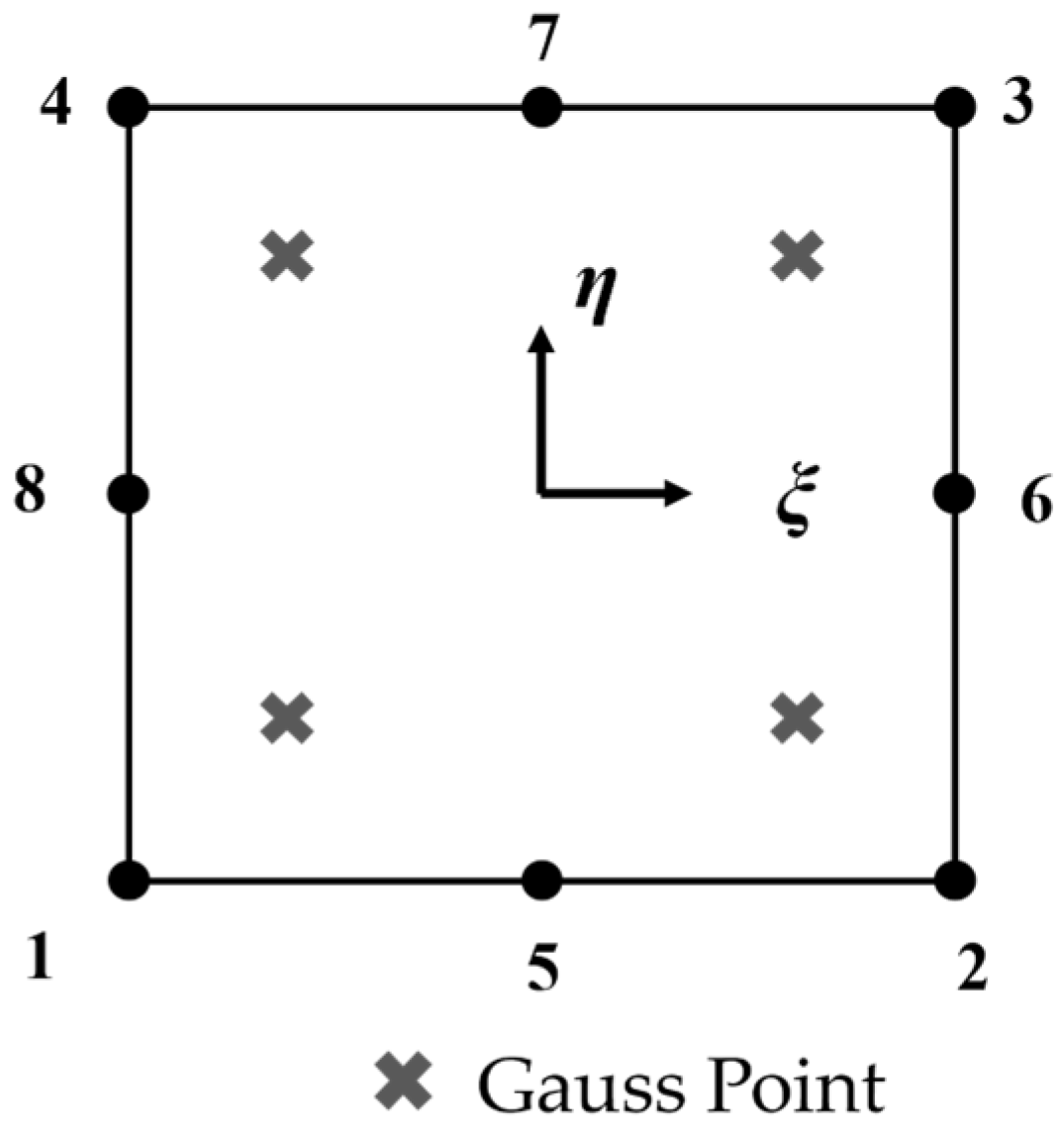
2.2. Element Formulation

Use the finite element method to interpolate the unknown functions:

$$u=Nq$$

(5)

where $u={[\begin{array}{ccccccc}{u}_0& v_0& w_0& {\phi }_x& {\phi }_y& \psi & \zeta \end{array}]}^T$, q is the nodal displacement vector, and N is the shape function matrix.

$$N_{(7\times 56)}=\left[\begin{array}{cccc}diag(N_1)& diag(N_2)& \dots & diag(N_8)\end{array}\right]$$

(6)

The potential energy of the element can be derived by:

$${\mathsf{\Pi }}^e={\displaystyle \frac{1}{2}}{q^e}^T{K}^e{q}^e-{F^e}^T{q}^e$$

(7)

with

$$K^e={{\displaystyle {\int }_{A}B}}^T{Q}_{0}BdA$$

(8)

where the superscript e means element, ${\mathit{K}}^{\mathit{e}}$ is the element stiffness matrix, ${\mathit{F}}^{\mathit{e}}$ is the nodal force vector of nodes, and $\mathit{B}=\mathit{L}·\mathit{N}$, is the strain-displacement matrix (see Appendix A for L). Using the minimum potential energy theorem, the equilibrium relation of the element is obtained:

$$K^e{q}^e=F^e$$

(9)

In the present work, an eight-node serendipity element, as shown in Figure 2, is used. The shape function is:

$$\begin{array}{l}{N}_1=-{\displaystyle \frac{1}{4}}(1-\xi )(1-\eta )(1+\xi +\eta );N_2=-{\displaystyle \frac{1}{4}}(1+\xi )(1-\eta )(1-\xi +\eta );\\ N_3=-{\displaystyle \frac{1}{4}}(1+\xi )(1+\eta )(1-\xi -\eta );N_4=-{\displaystyle \frac{1}{4}}(1-\xi )(1+\eta )(1+\xi -\eta );\\ N_5={\displaystyle \frac{1}{2}}(1-\xi )(1+\xi )(1-\eta );N_6={\displaystyle \frac{1}{2}}(1-\eta )(1+\eta )(1+\xi );\\ N_7={\displaystyle \frac{1}{2}}(1-\xi )(1+\xi )(1+\eta );N_8={\displaystyle \frac{1}{2}}(1-\eta )(1+\eta )(1-\xi )\end{array}$$

(10)

The integral of Equation (8) is calculated using Gaussian quadrature in a parametric element. Four Gauss points are used in the present element.

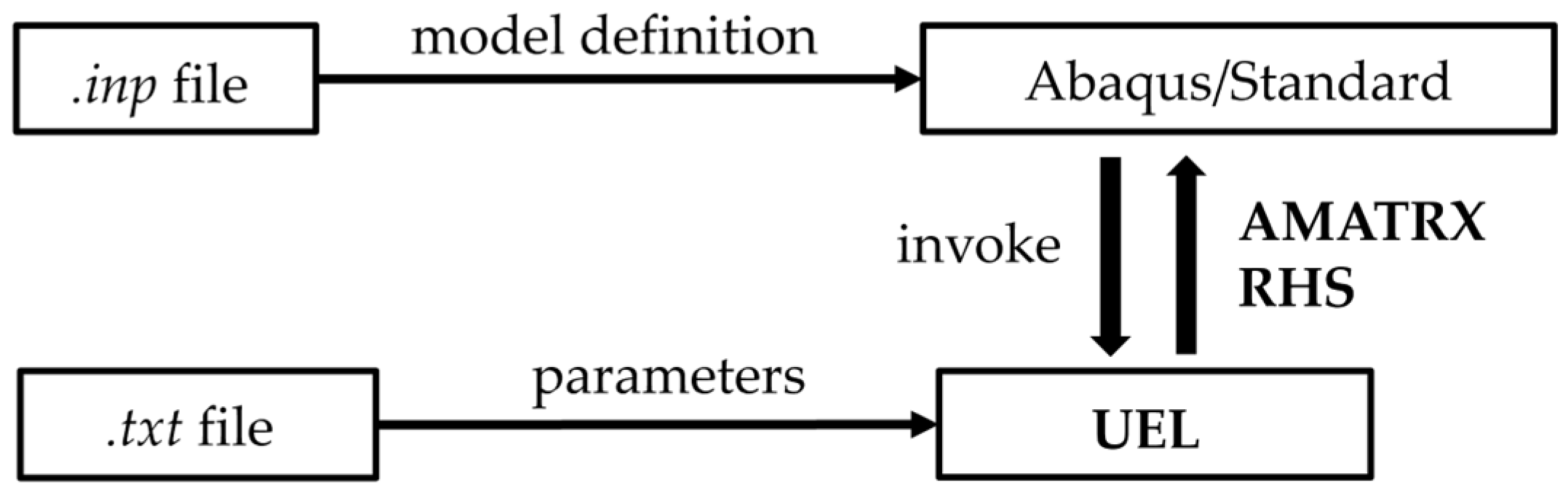
2.3. Implementation in Abaqus

Abaqus provides a user subroutine interface for advanced customization. Within Abaqus Standard, users can implement custom elements via the subroutine UEL. During analysis, Abaqus invokes UEL for each user element to retrieve elemental matrices (e.g., stiffness and mass matrices). The subroutine is written in Fortran (.for file extension), with function header and variable definitions detailed in the Abaqus documentation [16].

• Environment

Compilation environment configuration is a prerequisite for UEL implementation, which can vary across Abaqus versions. This study employs Abaqus 2022, Visual Studio 2019, and Intel Visual Fortran 2020. By default, UEL subroutines compile with the Fortran 77 fixed format; free-format Fortran (adopted in this work) requires configuration file modifications (see Appendix B).

• Programming guidelines

Comprehensive UEL guidelines can be found in references [25,26,27]. Some critical variables warrant emphasis here:

AMATRX: Represents the stiffness matrix (K) in static analyses.

U: Solution vector of nodal displacement, corresponding to q in Equation (5).

RHS: The residual vector. For linear elastic analysis, RHS = −AMATRX∙U.

Programming templates and reusable subroutines are provided in reference [30]; several of them are utilized in this work.

• Data flow

The data flow is illustrated in Figure 3. For each user-defined element, the UEL subroutine is invoked by the solver to provide the element stiffness matrix and residual vector. Two keywords are necessary in the .inp file:

*User Element: defines the element in DOFs and nodal configuration.

*Uel Property: passes parameters to UEL via the PROPS array.

In the present work, six REAL-type numbers are passed in to specify the material’s principal and normal vectors. Additional material properties and geometry parameters are read by UEL from a custom .txt file in the working directory.

• Activation of DOFs

The nodal DOFs in Abaqus follow a convention that DOFs 1–6 represent three translational and three rotational components [16]. For the plate element developed in this paper, it is necessary to activate DOFs 1–5. Since users cannot define additional DOFs in Abaqus, existing DOFs must be repurposed with their original meanings overridden—a methodology aligned with established practices [25,26,27]. Specifically, DOFs 11 and 12 (originally designated for temperature) are reassigned to represent ψ and ζ. To accommodate these repurposed DOFs, the coupled temperature-displacement analysis mode is selected for the load step. The field variable NT is added to the output. Output values NT11 and NT12 correspond DOFs 11 and 12, respectively.

• Element visualization

The user element cannot be visualized like the native elements. The solution is to superimpose a native element S8R with negligible stiffness on the user element, where two elements share the same nodes—these are called dummy elements. This is done by first modeling with S8R, then modifying the .inp file (see Appendix C). Loads and boundary conditions are applied according to specific problem requirements. Since DOFs 11 and 12 are assigned to DOFs ψ and ζ, their corresponding loads are applied via the keyword *Cflux. The user element does not support the *Surface keyword, but after using the dummy element, distributed loads can be applied directly to it. Uniformly distributed loads can alternatively be converted to nodal loads according to reference [30]. More complex distributed loads can be applied using the subroutine DLOAD, and custom boundary conditions can be defined using the subroutine DISP. These subroutines can be put in the same .for file without blanking lines between codes.

The source code of the UEL subroutines developed in this paper is available (see Data Availability Statement). These subroutines can be executed either through Abaqus/CAE or via the command terminal. The template command is: “abaqus job=jobname.inp user=subroutine.for”.

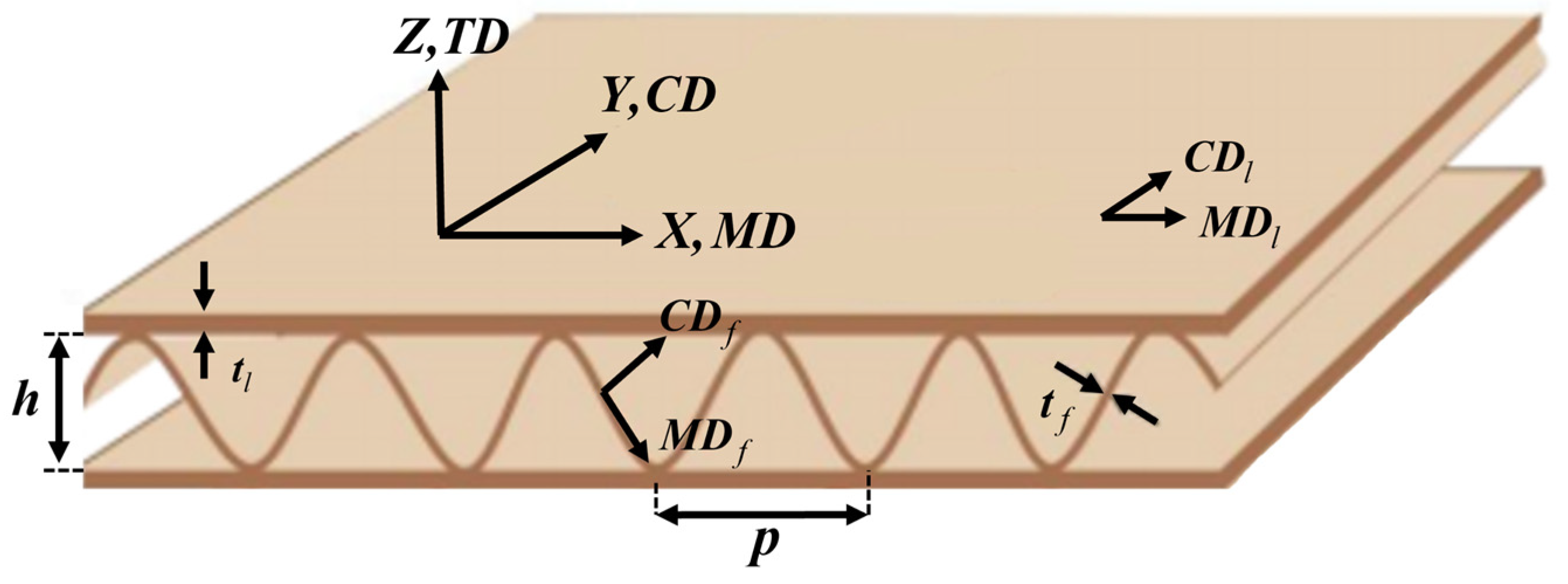
3. Extended Homogenization Method

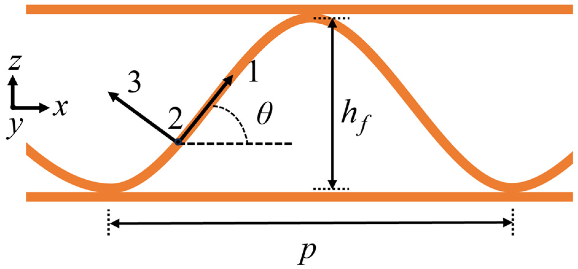
3.1. Extension on FSDT

The ideology of the FSDT homogenization method is based on coordinate transformation. As shown in Figure 4, the elastic constants of the flute are measured in its local coordinate system (123), rotated by an angle θ relative to the global coordinate system (xyz). The 1-direction represents the tangential direction of the flute.

Assuming the flute profile is modeled as a sinusoidal function, we have:

$$g(x)={\displaystyle \frac{h_f}{2}}\sin ({\displaystyle \frac{2\pi x}{p}})$$

(11)

$$\theta (x)={\tan }^{-1}({\displaystyle \frac{dg(x)}{dx}})$$

(12)

The transformation of stress and strain under coordinate rotation is governed by:

$$\left\{\begin{array}{c}{\epsilon }_{11}\\ {\epsilon }_{22}\\ {\epsilon }_{33}\\ {\gamma }_{23}\\ {\gamma }_{13}\\ {\gamma }_{12}\end{array}\right\}=\left[\begin{array}{cccccc}{c}^2& 0& s^2& 0& cs& 0\\ 0& 1& 0& 0& 0& 0\\ s^2& 0& c^2& 0& -cs& 0\\ 0& 0& 0& c& 0& -s\\ -2cs& 0& 2cs& 0& c^2-s^2& 0\\ 0& 0& 0& s& 0& c\end{array}\right]\left\{\begin{array}{c}{\epsilon }_{xx}\\ {\epsilon }_{yy}\\ {\epsilon }_{zz}\\ {\gamma }_{yz}\\ {\gamma }_{xz}\\ {\gamma }_{xy}\end{array}\right\}$$

(13)

$$\left\{\begin{array}{c}{\sigma }_{11}\\ {\sigma }_{22}\\ {\sigma }_{33}\\ {\tau }_{23}\\ {\tau }_{13}\\ {\tau }_{12}\end{array}\right\}=\left[\begin{array}{cccccc}{c}^2& 0& s^2& 0& 2cs& 0\\ 0& 1& 0& 0& 0& 0\\ s^2& 0& c^2& 0& -2cs& 0\\ 0& 0& 0& c& 0& -s\\ -cs& 0& cs& 0& c^2-s^2& 0\\ 0& 0& 0& s& 0& c\end{array}\right]\left\{\begin{array}{c}{\sigma }_{xx}\\ {\sigma }_{yy}\\ {\sigma }_{zz}\\ {\tau }_{yz}\\ {\tau }_{xz}\\ {\tau }_{xy}\end{array}\right\}$$

(14)

or in compact form:

$$\begin{array}{l}{\epsilon }_{123}=T_{\epsilon }{\epsilon }_{xyz}\\ {\sigma }_{123}=T_{\sigma }{\sigma }_{xyz}\end{array}$$

(15)

where $c=cos\theta$ and $s=sin\theta$. The constitutive relation is described as:

$$\begin{array}{l}{\epsilon }_{123}=S_{123}{\sigma }_{123}\\ {\epsilon }_{xyz}=S_{xyz}{\sigma }_{xyz}\end{array}$$

(16)

where S represents the compliance matrix:

$$S_{123}=\left[\begin{array}{cccccc}1/E_1& -{\nu }_{21}/E_2& 0& -{\nu }_{31}/E_3& 0& 0\\ -{\nu }_{12}/E_2& 1/E_2& 0& -{\nu }_{32}/E_3& 0& 0\\ 0& 0& 1/G_{12}& 0& 0& 0\\ -{\nu }_{13}/E_3& -{\nu }_{23}/E_3& 0& 1/E_3& 0& 0\\ 0& 0& 0& 0& 1/G_{13}& 0\\ 0& 0& 0& 0& 0& 1/G_{23}\end{array}\right]$$

(17)

Applying Equation (15) to Equation (16), one can get:

$$S_{xyz}=T_{\epsilon }^{-1}{S}_{123}{T}_{\sigma }$$

(18)

Notice that

$$T_{\epsilon }^{-1}=T_{\sigma }^T$$

(19)

A transformation of the constitutive relation can be obtained:

$$S_{xyz}=T_{\sigma }^T{S}_{123}{T}_{\sigma }$$

(20)

Equations (16)–(20) are the foundation of existing homogenization approaches, which gives transformation to the compliance matrix S, yet the ultimate objective should be the elastic matrix Q. Consequently, in references [7,10], the researchers first derived the modulus form compliance matrix using Equation (17), then substituted them into the elastic matrix of the planar form:

$$Q_{FSDT}=\left[\begin{array}{ccccc}{\displaystyle \frac{E_1}{1-{\nu }_{12}{\nu }_{21}}}& {\displaystyle \frac{{\nu }_{21}{E}_1}{1-{\nu }_{12}{\nu }_{21}}}& & & \\ {\displaystyle \frac{{\nu }_{12}{E}_2}{1-{\nu }_{12}{\nu }_{21}}}& {\displaystyle \frac{E_2}{1-{\nu }_{12}{\nu }_{21}}}& & & \\ & & G_{12}& & \\ & & & G_{13}& \\ & & & & G_{23}\end{array}\right]$$

(21)

Only 5 components of stress are needed in FSDT (3 for CLPT), whereas Equation (20) employs a full 3D constitutive relation containing all 6 stress components. This is an indirect approach that may have some flaws in the reasoning.

However, in the case of the present work, due to a higher order expansion in the displacement field, a full 3D constitutive relation is required, therefore transformation of the elastic matrix can be derived directly. Rewrite Equations (16)–(20) in a similar manner:

$$\begin{array}{l}{\sigma }_{123}=Q_{123}{\epsilon }_{123}\\ {\sigma }_{xyz}=Q_{xyz}{\epsilon }_{xyz}\end{array}$$

(22)

$$Q_{xyz}=T_{\sigma }^{-1}{Q}_{123}{T}_{\epsilon }$$

(23)

A relation similar to Equation (19) $T_{\sigma }^{-1}=T_{\epsilon }^T$ is also satisfied, one can get:

$$Q_{xyz}=T_{\epsilon }^T{Q}_{123}{T}_{\epsilon }$$

(24)

Notice that the 3D elastic matrix Q has a more complicated expression than the compliance matrix and Equation (21), but this can be numerically solved via the inverse of the compliance matrix S.

Substituting the elastic matrix into Equation (3) and applying the laminated plate theory, the integral along the whole thickness turns into the sum of each ply:

$$\begin{array}{l}A(x)={\displaystyle \sum _{k=1}^n{Q}_k{t}_k}\\ B(x)={\displaystyle \sum _{k=1}^n{Q}_k{z}_k{t}_k}\\ C(x)={\displaystyle \sum _{k=1}^n{Q}_k\left({z_k}^2{t}_k+\frac{{t_k}^3}{12}\right)}\\ D(x)={\displaystyle \sum _{k=1}^n{Q}_k\left({z_k}^3{t}_k+\frac{z_k{t_k}^3}{4}\right)}\\ E(x)={\displaystyle \sum _{k=1}^n{Q}_k\left({z_k}^4{t}_k+\frac{{z_k}^2{t_k}^3}{2}+\frac{{t_k}^5}{80}\right)}\end{array}$$

(25)

where subscript k stands for the kth layer, t means the thickness of paper sheet, z means the distance to the middle surface of the whole laminated plate. If the kth layer is a liner, then $t_k$, $z_k$, and ${\mathit{Q}}_k$ will be constant; otherwise (for a flute) $t_k=t_f/cos\theta$, $z_k$ refers to Equation (11) and ${\mathit{Q}}_k$ refers to Equation (24). Therefore, the matrices are dependent on x (θ is a function of x). To eliminate the dependency on x, the constitutive matrix is finally averaged over a period of x.

$$\left[\begin{array}{ccccc}A& B& C& D& E\end{array}\right]={\displaystyle \frac{1}{p}}{\displaystyle {\int }_0^p\left[\begin{array}{ccccc}A(x)& B(x)& C(x)& D(x)& E(x)\end{array}\right]}dx$$

(26)

These integrals are complex and need to be evaluated numerically, e.g., using trapezoid rule integration. The procedures above are applicable from single-wall to multi-wall corrugated cardboards.

3.2. Correction on Out-of-Plane Stiffness

Corrugated cardboard is more complex than a laminated plate due to the cavities, and the coordinate transformation is a kind of mathematic derivation, which can be improved by mechanical analysis. Therefore, a correction to the out-of-plane stiffness is developed by treating the flute as a three-hinged arch here.

As shown in Figure 5, the corrugated shape is approximately sinusoidal, with a concentrated load at the center hinge. The three-hinged arch is a statically determinate structure, so its reaction forces and internal forces can be directly obtained by solving the equilibrium equations.

$$\begin{array}{cc}{F}_{ly}=F_{ry}={\displaystyle \frac{F}{2}};& F_{lx}=F_{rx}={\displaystyle \frac{pF}{4h_f}}\end{array}$$

(27)

$$M=\left\{\begin{array}{c}\hspace{1em}\hspace{1em}\begin{array}{cc}{\displaystyle \frac{F}{2}}x-{\displaystyle \frac{Fp}{4h_f}}g(x),& 0\le x\le {\displaystyle \frac{p}{2}}\end{array}\\ \begin{array}{cc}{\displaystyle \frac{F}{2}}x-{\displaystyle \frac{Fp}{4h_f}}g(x)-F(x-{\displaystyle \frac{p}{2}}),& {\displaystyle \frac{p}{2}}<x\le p\end{array}\end{array}\right.$$

(28)

$$N=\left\{\begin{array}{c} \begin{array}{cc}-{\displaystyle \frac{F}{2}}\sin \theta -{\displaystyle \frac{Fp}{4h_f}}\cos \theta ,& 0\le x\le {\displaystyle \frac{p}{2}}\end{array}\\ \begin{array}{cc}{\displaystyle \frac{F}{2}}\sin \theta -{\displaystyle \frac{Fp}{4h_f}}\cos \theta ,& {\displaystyle \frac{p}{2}}<x\le p\end{array}\end{array}\right.$$

(29)

$$T=\left\{\begin{array}{c}\begin{array}{cc}{\displaystyle \frac{F}{2}}\cos \theta -{\displaystyle \frac{Fp}{4h_f}}\sin \theta ,& 0\le x\le {\displaystyle \frac{p}{2}}\end{array}\\ \begin{array}{cc}{\displaystyle \frac{F}{2}}\cos \theta +{\displaystyle \frac{Fp}{4h_f}}\sin \theta ,& {\displaystyle \frac{p}{2}}<x\le p\end{array}\end{array}\right.$$

(30)

where M, N, and T represent the internal moment, axial, and shear force, respectively. The term g(x) refers to Equation (11).

According to Castigliano’s theorem, the displacement Δ corresponding to F can be obtained by:

$$\Delta ={\displaystyle \int \frac{M}{EI}\cdot \frac{\partial M}{\partial F}ds}+{\displaystyle \int \frac{N}{EA}\cdot \frac{\partial N}{\partial F}ds}+{\displaystyle \int \frac{kT}{GA}\cdot \frac{\partial T}{\partial F}ds}$$

(31)

where the right-hand side terms correspond to the contribution of flexural, axial, and sheer deformation, respectively. The term ds is the differential element of arc length; in Cartesian coordinates: $ds=\sqrt{1+g^{\prime 2}}dx$. E is Young’s modulus, G is the shear modulus, I is moment of inertial I = t³/12, A = t is the sectional area, and k is the shear correction coefficient.

Since bending dominates in this load case, the last two terms can be discarded for simplicity. Additionally, symmetry can be exploited to avoid piecewise functions. Thus, we obtain:

$$\Delta =2{\displaystyle {\int }_0^{p/2}\frac{F(\frac{x}{2}-\frac{p}{4h_f}g(x){)}^2}{EI}\sqrt{{1+g{(x)}^{\prime }}^2}dx}$$

(32)

where F is arbitrary and can be set to 1. The integral can be evaluated numerically.

Then a nominal equivalent modulus can be calculated as:

$$E_z={\displaystyle \frac{h_{f}F}{p\Delta }}$$

(33)

This homogenized modulus is directly related to A₃₃, B₃₃, and C₃₃ in Equation (2). Therefore we can use it to correct these three terms. While substituting E_z into Q₃₃ is feasible, the explicit form of the 3D elastic stiffness matrix Q is complicated due to Poisson’s ratio. However, a simplification is given here, because on one hand the derivation above is inherently uniaxial, and on the other hand work by Fadiji [31] indicates that these effects are small. Consequently, it is reasonable to replace Q₃₃ with E_z. Replace t_k in Equation (25) with h, since we have homogenized the flute. We thus obtain:

$$\begin{array}{l}{A}_{33}^f=E_{z}h\\ B_{33}^f=E_z{z}_{k}h\\ C_{33}^f=E_z(z_k^{2}h+h^3/12)\end{array}$$

(34)

For single-wall corrugated cardboard, $z_k=0$ due to symmetry. The rest of the matrix terms remain unchanged as calculated via the procedures in Section 3.1. Validation in Section 4.3 demonstrates that this scheme performs effectively.

4. Validation

Tests were designed to verify the correctness of element programming and whether it could achieve the intended goals.

4.1. Patch Test

A patch test is performed to assess the element’s ability to represent a constant strain state, which is necessary for element convergence. As illustrated in Figure 6a, a central element is surrounded by four elements. A displacement field of $u=0.01x$, $v=-0.003y$ is assumed, from which nodal displacements can be obtained in

Table 2. Nodal displacements of patch test.

Node ID	x-Coordinate	y-Coordinate	u	v
1	0	0	0	0
2	2.5	0	0.025	0
3	2.5	3	0.025	−0.009
4	0	2	0	−0.006
5	0.5	0.5	0.005	−0.0015
6	2	0.75	0.02	−0.00225
7	1.75	1.75	0.0175	−0.00525
8	0.65	1.6	0.0065	−0.0048
9	1.25	0	0.0125	0
10	2.5	1.5	0.025	−0.0045
11	1.25	2.5	0.0125	−0.0075
12	0	1	0	−0.003
13	1.25	0.625	0.0125	−0.001875
14	1.875	1.25	0.01875	−0.00375
15	1.2	1.675	0.012	−0.005025
16	0.575	1.05	0.00575	−0.00315
17	2.25	0.375	0.0225	−0.001125
18	2.125	2.375	0.02125	−0.007125
19	0.325	1.8	0.00325	−0.0054
20	0.25	0.25	0.0025	−0.00075

. If the element satisfies basic consistency and completeness requirements, then when nodal displacements are applied on the outside nodes (red dots in Figure 6a), the displacements of inner nodes (blue dots) should match the predefined field exactly. Material properties are defined as isotropic elastic with a Young’s modulus $E=1000$ MPa and Poisson’s ratio $\nu =0.3$.

The result is shown in Figure 6c, which is totally identical to the result from Abaqus native element S8R in Figure 6b, confirming that the proposed element passes the patch test.

4.2. Homogeneous Plate

In the case of a bi-sinusoidal load, $q=q_0\sin \left(\pi x/a\right)\sin \left(\pi y/b\right)$ applied to a rectangular plate with four simply supported edges is examined. Parameters are set as: $a=b=100$ mm, span-to-thickness ratio $a/h=10$, $q_0=1$ N. The material of the plate is isotropic, $E=2\times {10}^5$ MPa, $\nu =0.3$.

Simulation results from different elements, including solid element C3D8R, continuum shell element SC8R, conventional shell S8R, and the proposed element are compared in Figure 7, Figure 8 and Figure 9. The continuum shell element is a brick element analogous to a solid element in modeling but theoretically based on shell theory [16]. A continuum shell can be discretized in a single or stacked layers. There are 10 layers of element, solid element, and continuum shell stacked in the thickness direction to ensure accuracy, which can be a benchmark for the proposed element.

Figure 7 shows the comparison of maximum deflections. The maximum deflection of this problem occurs at the center of the plate. The result from the proposed element is almost identical to the result from S8R, which is reasonable because the proposed element is developed from FSDT. Results from these two elements are slightly smaller (about 2%) than those from C3D8R and SC8R, which might be caused by the linear simplification of transverse shear in S8R and the proposed element.

Figure 8 shows the distribution of the transverse normal strain ${\epsilon }_z$ along the thickness of various elements at x = 75 mm, y = 75 mm. The ${\epsilon }_z$ of the proposed element is linearly distributed, which gives better characterization than the conventional shell S8R (zero) and the single-layer continuum shell SC8 R (constant distribution). Compared with the stacked SC8R and the solid C3D8R, the ${\epsilon }_z$ distribution of the proposed element aligns closely, except near the top and bottom surface, demonstrating sufficient accuracy for the linear characterization of transverse normal strain.

Figure 9 shows the distribution of the transverse normal stress ${\sigma }_z$. It can be observed that ${\sigma }_z$ exhibits a linear distribution, as the strain does. However, it does not fully match the results from the C3D8R and stacked SC8R elements as ${\sigma }_z$ follows a cubic distribution [32]. While increasing the order of z in the displacement field could potentially resolve this discrepancy, it would also increase the model’s complexity. The proposed element provides a balanced solution with its linear distribution. Notice that the stress values at the middle surface (z = 0) and the top and bottom surfaces (z = ±5) show good agreement, verifying the correctness of the proposed element.

4.3. Homogenized Model for Corrugated Cardboard

The detailed finite element model of a single-wall corrugated cardboard is established in Abaqus using S4R elements and compared with the homogenized model using the proposed element. The flutes and liners of the detailed model are bonded by sharing the same nodes. The material and geometry parameters are shown in

Table 3. Elastic property of raw paper.

Layer	Thickness (mm)	Elastic Constant (MPa)						Period (mm)	Height (mm)
		E1	E2	ν12	G12	G13	G23
Liner	0.29	3326	1694	0.34	860	60	48	--	--
Flute	0.30	2614	1532	0.33	792	47	43	8	4

. The size of the model is 80 mm × 80 mm × 4 mm, and it contains 10 complete corrugated periods in MD.

Different load cases including stretching, bending, twisting, and shearing on MD and CD are applied to the detailed model and the homogenized model. Kinematic coupling constraints are used on the boundary of both models to apply consistent boundary conditions and loads. The displacement results on the control point are shown in

Table 4. Displacement comparison of homogenized and detailed model in different load cases.

Load Case	Displacement *	Detailed Model	Homogenized Model	Error
MD-bending	U3	4.7805 × 10−1	4.6394 × 10−1	−2.95%
CD-bending	U3	7.2503 × 10−1	7.1266 × 10−1	−1.71%
MD-stretching	U1	4.7967 × 10−2	4.7894 × 10−2	−0.15%
CD-stretching	U2	5.6697 × 10−2	5.6701 × 10−2	0.01%
MD-twisting	UR1	8.9073 × 10−3	8.2304 × 10−3	−7.60%
CD-twisting	UR2	7.7143 × 10−3	7.2510 × 10−3	−6.01%
CD-shearing	U2	2.1472 × 10−1	2.2272 × 10−1	3.72%
MD-shearing	U1	2.2251 × 10−1	2.3330 × 10−1	4.85%

* U and UR correspond to translational displacement and rotation in Abaqus.

. It can be seen that the overall error between the detailed model and the homogenized model is within 8%, indicating that the extended homogenization method is accurate. Figure 10 compares contour plots of both models under CD bending. The homogenized model demonstrates excellent global consistency with the detailed model; a refined mesh is unnecessary. The user element can be visualized like native elements thanks to dummy elements. Otherwise, only thin cross lines would be seen in Figure 10.

Table 5. Runtime of homogenized and detailed model in CD-bending simulation.

Name	Element Number	Node Number	Total DOFs	Runtime (s)	Reduction
Detailed model	14,400	13,542	81,252	1.8	--
Homogenized model	338	560	3920	0.8	55.56%

compares the computational scale and runtime of both models in a CD-bending simulation. The size of equations systems to be solved directly relates to the number of total DOFs, which drops massively when using a homogenized model. Therefore, the runtime can be reduced by over 50%, significantly enhancing the FEA efficiency of corrugated cardboard. The load case selected for comparison here is basic and the model scale remains relatively small, with most of the computational time spent on preprocessing. Therefore, this efficiency gain can be viewed as a conservative baseline; it will become more pronounced for larger-scale models.

To evaluate through-thickness deformation, displacements along the line y = 40 mm in the CD-bending simulation are extracted and plotted in Figure 11. Thickness reduction in the detailed model is calculated as the deflection difference between corresponding nodes on the upper and lower liners. The curve in Figure 11 exhibits significant fluctuations due to the local warping of the liners, which is particularly pronounced near boundaries caused by insufficient constraints; nevertheless, the thickness is reduced overall as expected. Based on the displacement field assumption, the thickness reduction in the proposed element is defined as hψ. Figure 11 demonstrates that the proposed element accurately captures the average thickness reduction of the detailed model.

Additionally, to directly evaluate the element’s capability in characterizing through-thickness deformation, an out-of-plane compression test was conducted. The loading and boundary conditions were applied as follows: for the detailed model, the bottom liner was fully constrained while the top liner was coupled to a control point under concentrated loading. For the homogenized model, all nodal DOFs except ψ and ζ were constrained, with a uniformly distributed load applied. Although the displacement DOFs are constrained, thickness-direction deformation can be still captured through DOF ψ and ζ.

Figure 12 shows the resulting nominal stress-strain curves. The out-of-plane stiffness from the proposed method matches the detailed model well in the linear stage, validating the correction on the out-of-plane stiffness. As strain increases, the buckling of the flute induces nonlinear behavior, revealing limitations of the linear elastic constitutive model used in this paper. Nevertheless, the element inherently characterizes out-of-plane deformation, and elastoplastic constitutive relationships may be implemented in future work.

5. Conclusions and Discussion

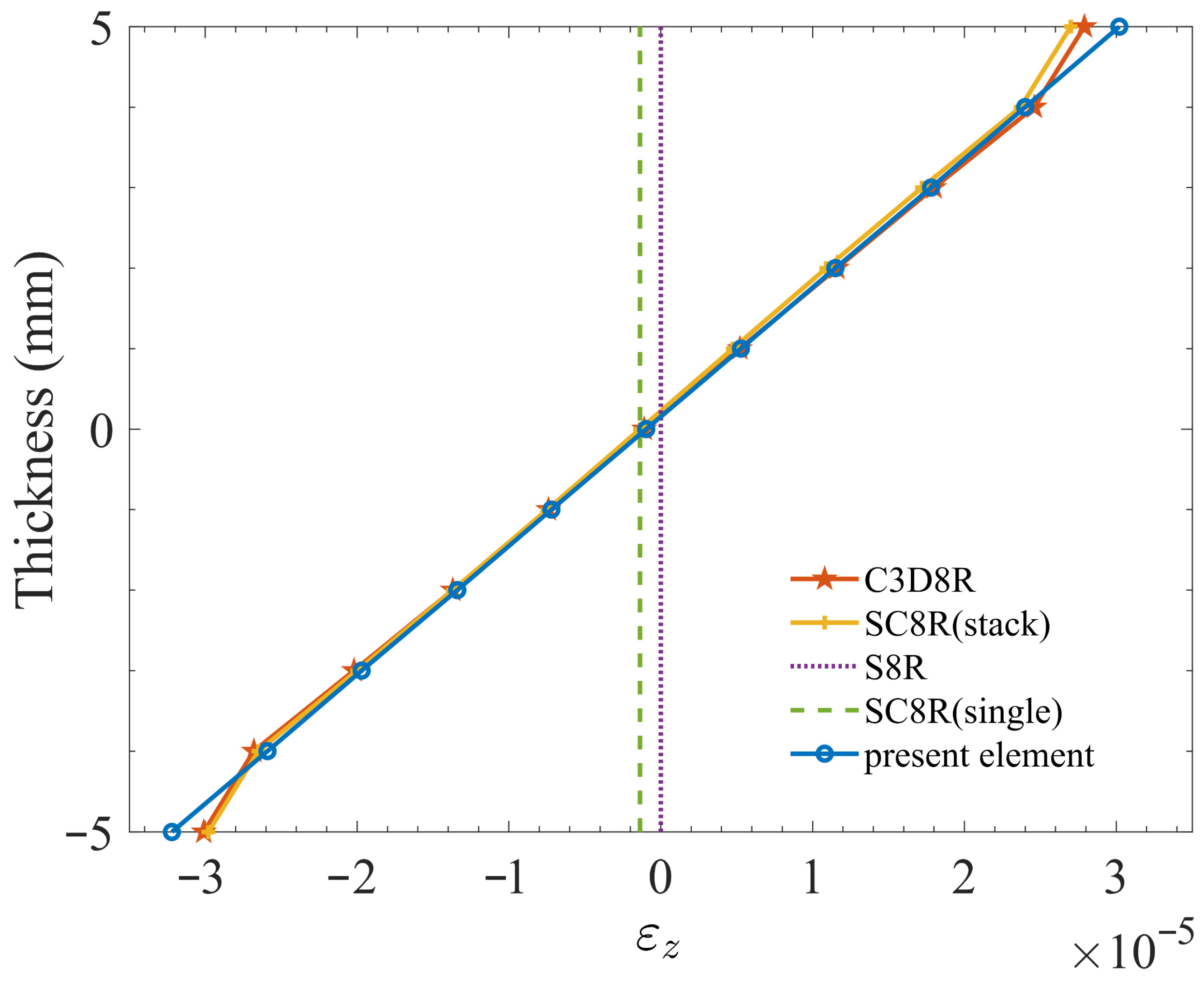
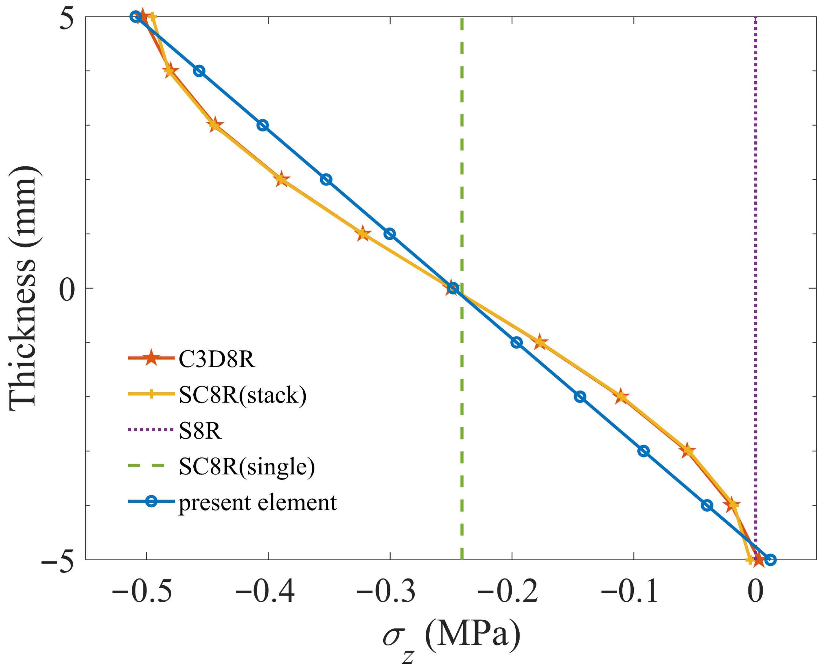
In order to characterize the through-thickness deformation in the homogenization of corrugated cardboard, this paper develops a plate element that incorporates transverse normal strain and extends established homogenization methods. The main conclusions are as follows:

(1)

The plate element, implemented through the user subroutine UEL in Abaqus 2022, can pass the patch test. The transverse normal strain and stress are linearly distributed along the thickness direction, which is consistent with results from the Abaqus native elements S8R, SC8R, and C3D8R.

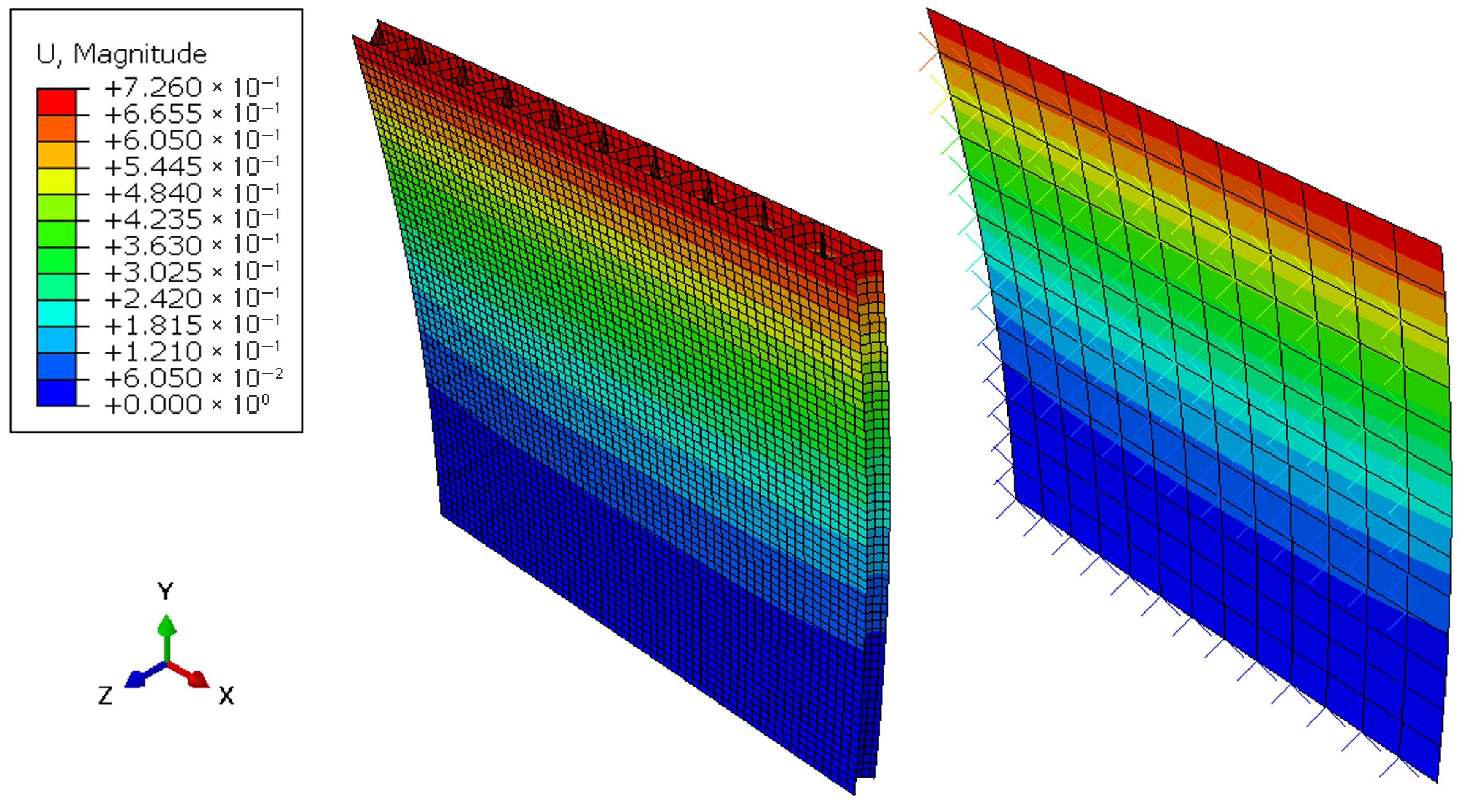
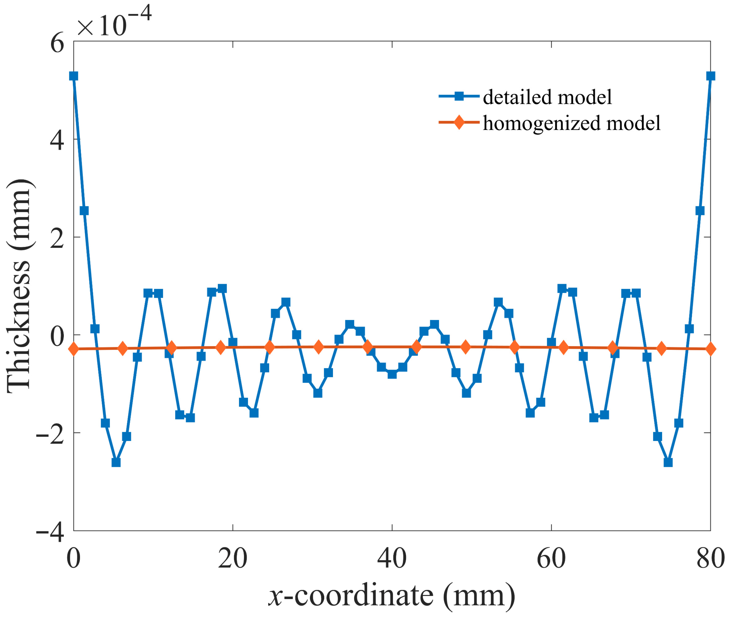
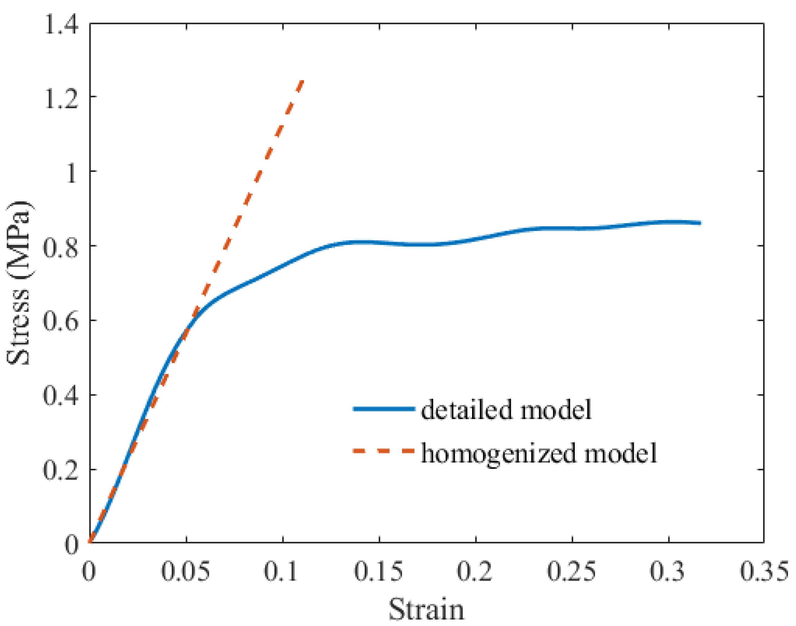
(2)

By developing extensions to the established homogenization method and improving the out-of-plane stiffness, results from the homogenized model are well matched to the detailed model, with an error of less than 8% and a runtime reduction of more than 50%. The stress-strain relation of the homogenized model shows good agreement in the linear stage on the out-of-plane compression test, showing the correctness of the proposed method and the limitations of the linear elastic constitutive model.

There are some drawbacks of this work that can be improved in further researches. (a) Despite being compatible with Abaqus, the presented element requires many manual modifications to files, and the degrees of automation and convenience in its use could be improved. (b) More complicated constitutive relations such as nonlinearity, the effects of heat and humidity, strain rates, etc., should be integrated. (c) More numerical and experimental tests under real-life situations need to be conducted to verify the correctness and reliability of the element.

References

1. Briassoulis, D. Equivalent orthotropic properties of corrugated sheets. Comput. Struct. 1986, 23, 129–138. [Google Scholar] [CrossRef]
2. Biancolini, M.E.; Brutti, C.; Porziani, S. Corrugated board containers design methods. Int. J. Comput. Mater. Sci. Surf. Eng. 2010, 3, 143–163. [Google Scholar] [CrossRef]
3. Nordstrand, T.; Carlsson, L.A.; Allen, H.G. Transverse shear stiffness of structural core sandwich. Compos. Struct. 1994, 27, 317–329. [Google Scholar] [CrossRef]
4. Bartolozzi, G.; Pierini, M.; Orrenius, U.; Baldanzini, N. An equivalent material formulation for sinusoidal corrugated cores of structural sandwich panels. Compos. Struct. 2013, 100, 173–185. [Google Scholar] [CrossRef]
5. Abbès, B.; Guo, Y.Q. Analytic homogenization for torsion of orthotropic sandwich plates: Application to corrugated cardboard. Compos. Struct. 2010, 92, 699–706. [Google Scholar] [CrossRef]
6. Aboura, Z.; Talbi, N.; Allaoui, S.; Benzeggagh, M.L. Elastic behavior of corrugated cardboard: Experiments and modeling. Compos. Struct. 2004, 63, 53–62. [Google Scholar] [CrossRef]
7. Talbi, N.; Batti, A.; Ayad, R.; Guo, Y.Q. An analytical homogenization model for finite element modelling of corrugated cardboard. Compos. Struct. 2009, 88, 280–289. [Google Scholar] [CrossRef]
8. Minh, D.P.T. Modeling and Numerical Simulation for the Double Corrugated Cardboard under Transverse Loading by Homogenization Method. Int. J. Eng. Sci. 2017, 6, 16–25. [Google Scholar]
9. Aduke, R.N.; Venter, M.P.; Coetzee, C.J. An Analysis of Numerical Homogenisation Methods Applied on Corrugated Paperboard. Math. Comput. Appl. 2023, 28, 46. [Google Scholar] [CrossRef]
10. Suarez, B.; Muneta, M.L.M.; Sanz-Bobi, J.D.; Romero, G. Application of homogenization approaches to the numerical analysis of seating made of multi-wall corrugated cardboard. Compos. Struct. 2021, 262, 113642. [Google Scholar] [CrossRef]
11. Biancolini, M.E. Evaluation of equivalent stiffness properties of corrugated board. Compos. Struct. 2005, 69, 322–328. [Google Scholar] [CrossRef]
12. Garbowski, T. Computer aided estimation of corrugated board box compression strength Part 1: The Effect of Corrugated Cardboard Crushing on Its Basic Parameters. Przegląd Pap. 2018, 1, 47–54. [Google Scholar]
13. Krusper, A.; Isaksson, P.; Gradin, P. Modeling of Out-of-Plane Compression Loading of Corrugated Paper Board Structures. J. Eng. Mech. 2007, 133, 1171–1177. [Google Scholar] [CrossRef]
14. Huang, J. Investigation of Corrugated Cardboard for Vibration Isolation; University of Saskatchewan: Saskatoon, SK, Canada, 2013. [Google Scholar]
15. Wang, Z.W.; Yu-Ping, E. Energy absorption properties of multi-layered corrugated paperboard in various ambient humidities. Mater. Des. 2011, 32, 3476–3485. [Google Scholar] [CrossRef]
16. SIMULIA. Abaqus User Assistance. Available online: https://help.3ds.com/ (accessed on 27 April 2025).
17. ANSYS. ANSYS Documentation. Available online: https://ansyshelp.ansys.com/ (accessed on 27 April 2025).
18. Irfan, S.; Siddiqui, F. A review of recent advancements in finite element formulation for sandwich plates. Chin. J. Aeronaut. 2019, 32, 785–798. [Google Scholar] [CrossRef]
19. Bathe, K.J.; Dvorkin, E.N. A formulation of general shell elements—The use of mixed interpolation of tensorial components. Int. J. Numer. Methods Eng. 2005, 22, 697–722. [Google Scholar] [CrossRef]
20. Pandit, U.K.; Mondal, G.; Punera, D. Investigating the static, free vibration, and buckling responses of corrugated steel plate-made structures using efficient homogenization-based FE modelling. Structures 2024, 70, 107643. [Google Scholar] [CrossRef]
21. Djilali Hammou, A.; Minh Duong, P.T.; Abbès, B.; Makhlouf, M.; Guo, Y.-Q. Finite-element simulation with a homogenization model and experimental study of free drop tests of corrugated cardboard packaging. Mech. Ind. 2012, 13, 175–184. [Google Scholar] [CrossRef]
22. Carrera, E. Theories and Finite Elements for Multilayered Plates and Shells:A Unified compact formulation with numerical assessment and benchmarking. Arch. Comput. Methods Eng. 2003, 10, 215–296. [Google Scholar] [CrossRef]
23. Thai, H.T.; Choi, D.H. Finite element formulation of various four unknown shear deformation theories for functionally graded plates. Finite Elem. Anal. Des. 2013, 75, 50–61. [Google Scholar] [CrossRef]
24. Talha, M.; Singh, B.N. Static response and free vibration analysis of FGM plates using higher order shear deformation theory. Appl. Math. Model. 2010, 34, 3991–4011. [Google Scholar] [CrossRef]
25. Moreira, J.A.; Moleiro, F.; Araújo, A.L. Layerwise electro-elastic user-elements in Abaqus for static and free vibration analysis of piezoelectric composite plates. Mech. Adv. Mater. Struct. 2021, 29, 3109–3121. [Google Scholar] [CrossRef]
26. Moreira, J.A.; Moleiro, F.; Araújo, A.L.; Pagani, A. Assessment of layerwise user-elements in Abaqus for static and free vibration analysis of variable stiffness composite laminates. Compos. Struct. 2023, 303, 116291. [Google Scholar] [CrossRef]
27. Ferreira, G.F.O.; Almeida, J.H.S.; Ribeiro, M.L.; Ferreira, A.J.M.; Tita, V. Development of a finite element via Unified Formulation: Implementation as a User Element subroutine to predict stress profiles in composite plates. Thin-Walled Struct. 2020, 157, 107107. [Google Scholar] [CrossRef]
28. Nelson, R.B.; Lorch, D.R. A Refined Theory for Laminated Orthotropic Plates. J. Appl. Mech. 1974, 41, 177–183. [Google Scholar] [CrossRef]
29. Lo, K.H.; Christensen, R.M.; Wu, E.M. A High-Order Theory of Plate Deformation—Part 1: Homogeneous Plates. J. Appl. Mech. 1977, 44, 663–668. [Google Scholar] [CrossRef]
30. Smith, I.M.; Griffiths, D.V.; Margetts, L. Programming the Finite Element Method; John Wiley & Sons: Hoboken, NJ, USA, 2013. [Google Scholar]
31. Fadiji, T.; Ambaw, A.; Coetzee, C.J.; Berry, T.M.; Opara, U.L. Application of finite element analysis to predict the mechanical strength of ventilated corrugated paperboard packaging for handling fresh produce. Biosyst. Eng. 2018, 174, 260–281. [Google Scholar] [CrossRef]
32. Ventsel, E.; Krauthammer, T. Thin Plates and Shells: Theory, Analysis, and Applications; Marcel Dekker, Inc.: New York, NY, USA, 2002. [Google Scholar]
Figure 1. Principal directions of corrugated cardboard.
Applsci 15 07868 g001
Figure 2. Eight-node planar element.
Applsci 15 07868 g002
Figure 3. Data flow between main program and subroutine.
Applsci 15 07868 g003
Figure 4. The local and global coordinate system of the flute.
Applsci 15 07868 g004
Figure 5. Simplify the flute to a 3-hinged arch.
Applsci 15 07868 g005
Figure 6. Patch test regime (a) and result: S8R (b), proposed user element (c).
Applsci 15 07868 g006
Figure 7. Comparison of maximum deflection.
Applsci 15 07868 g007
Figure 8. The distribution of transverse normal strain.
Applsci 15 07868 g008
Figure 9. The distribution of transverse normal stress.
Applsci 15 07868 g009
Figure 10. Detailed model (left) and homogenized model using the proposed element (right).
Applsci 15 07868 g010
Figure 11. The thickness reduction in CD-bending simulation.
Applsci 15 07868 g011
Figure 12. The stress-strain relation in out-of-plane compression test.
Applsci 15 07868 g012