Numerical Study on Tree Belt Impact on Wind Shear on Agricultural Land

Abstract

Tree belts are commonly applied over agricultural terrain where seeds of wheat and other vegetation are planted in the ground in order to prevent the seeds from being blown by the wind. The tree belt comprises a long and thin (10–20 m thick) section of trees, which spans in a direction normal to the prevailing wind direction. While serving its agricultural goal, the belt does inevitably modify the boundary layer profile of the wind. This, on its part, is likely to affect the operation of small-scale wind turbines installed in the vicinity of the belt. The goal of this study is to determine the span and range at which this effect manifests itself. It was found that in the near vicinity downstream and slightly above the tree belt, the wind velocity actually increased due to the mass conservation. The flow became independent on the tree belt drag coefficient when its value was higher than 0.2 1/m. The turbulence introduced by the belt was restricted to a height of 1.5–2 tree belts.

1. Introduction

The tree belts play an important role in the sustainable management of agricultural landscapes, fulfilling multiple functions related to the environmental protection, improved agricultural productivity, and renewable energy support [1,2,3]. They are a key element in the soil erosion reduction, wind load protection, and agricultural microclimate improvements. However, scientific research often faces challenges related to quantitative modeling of their effect on the airflow, as well as the lack of empirical data for their characterization in different climatic conditions. The study in [4] focused on agroforestry as an effective strategy for sustainable agriculture and climate change mitigation, highlighting the need for integrated policies and research directions. The protective functions of tree belts, such as reducing wind speed and limiting soil erosion, have been documented by multiple authors [5,6,7]. Furthermore, these linear green structures modify the wind airflow, including the wind shear—a parameter that is critical for both agriculture and renewable energy systems, such as wind turbines [8,9,10]. According to the authors in [11], the transition to renewable energy sources, including wind power, requires strategic location planning to ensure environmental sustainability, energy efficiency, and public support.

The interaction between tree belts and wind flow has been studied in detail by the authors in [12,13,14,15], who highlighted the importance of these structures for wind profile modification and turbulence reduction. The interest in this aspect increases when the possibility of deploying wind turbines near the belts is considered. The authors in [16,17] pointed out that the efficiency of wind turbines depends significantly on the uniformity and turbulence of the velocity field. On the other hand, the presence of a tree belt has a direct impact on these parameters by creating zones of reduced velocity behind the belt and accelerated airflow above its height. This interaction significantly affects the aerodynamic characteristics of the wind turbine operating characteristics [18,19]. The authors in [20] emphasized that the alignment of tree belts perpendicular to the dominant wind direction (in their case, north–northwest) is crucial for the optimization of the protective and aerodynamic effects on the environment. This approach allows the creation of synergies between soil protection and energy efficiency gains.

Traditionally, the tree belts have been used to protect soil and crops from wind loads [21,22,23,24]. The authors in [25] found that these structures reduce the wind speed behind them by up to 60%, which significantly limits erosion and stabilizes the soil. Furthermore, studies in [26,27,28] showed that the tree belts increase soil moisture by reducing evaporation, which contributes to sustainable water resource management. However, modern research goes beyond traditional applications. The authors in [29,30,31] investigated the role of tree belts in modifying wind shear and aerodynamic airflow characteristics. An important contribution is the study in [32], which considered the forest farm-shelter network as a complex windbreak system. According to the analysis of the results, optimizing the spacing of the main shelterbelts upholds an efficiency of over 70%, while increasing the planting area, reducing side effects, and improving mechanized tillage and farming efficiency. This highlights the need for an in-depth study of the key airflow characteristics, such as wind shear, which are critical for sustainable and efficient agroecosystem management.

The wind shear, defined as the change in the wind speed with the height, plays a key role in the sustainable management of agroecosystems [33,34]. Research in [35] highlighted the importance of atmospheric stability for the accurate assessment of wind energy resources and recommended the necessity of more in-depth research on the impact of climate change on the stability of airflows in wind farms. The results of the studies in [36,37,38,39,40] indicated that the tree belts reduce the wind speed behind them and create accelerated airflow zones above their height. The analysis in [41] showed a model that investigates how the trees bend under wind forces, revealing that this reduces their zone of protection and changes the air movement around them. According to the findings in [14], these zones can be used strategically to protect crops and optimize the placement of wind turbines. More detailed studies in [42] showed that the structure of tree belts—density, height, and orientation relative to prevailing winds—has a significant influence on wind shear and agricultural conditions. The denser belts create strong turbulence, which can reduce erosion but harm some crops. From an energy point of view, the combined windbreaks in [43] (vegetated and artificial barriers) are more effective, arguing that there are plant species that significantly outperform natural plants at high wind speeds. Analysis through CFD and RANS simulations in [44,45,46,47,48,49] revealed optimal protection through a row of artificially planted bushes and highlighted the diversity in performance of different prediction models. Only one of the models in the study accurately predicted turbulence behind single-row barriers.

The study in [50] provided valuable information on the interaction of airflow with vegetation shelterbelts using CFD simulations with a k-ε model that successfully predicts flow characteristics but underlines the need to overcome limitations related to the accuracy of complex interactions. In [51], the challenges of modeling airflow in forest clear-cuts were highlighted, noticing the non-necessity of specific measures, such as increased wind turbine hub height to minimize turbulence and shear layers. The study in [52] evaluated the spectral tensor model of rapid distortion theory (RDT), which showed high accuracy in forested terrains under stable atmospheric conditions but struggled under unstable stratification. The analysis in [53] examined the performance of windbreaks through numerical simulations, highlighting the importance of parameters such as porosity and planting distance as optimal conditions for significant reduction of wind speed and erosion. In [54], a strategic combination of vegetation for sensible dryland management was investigated, but the study was limited to a specific geography and short observation period, which limits its applicability. The study in [17] analyzed the geometrical parameters of the shelter belts, showing that increasing the width and length improved the shelter effect, but increased the turbulence, while the presence of openings reduced the shelter area. The study in [55] proposed innovative indices to measure the performance of vegetated windbreaks using 3D CFD simulations that define optimal configurations for dry regions to reduce wind erosion and manage airflows.

The studies cited in [56,57,58,59,60] indicated that sparse tree belts promote a more uniform airflow, which is favorable for the installation of wind turbines. The study in [61] investigated the influence of turbulence spectral parameters on turbine loads, highlighting the significant influence of the anisotropy and the turbulence scale. The turbulence generated by tree belts is a key factor for wind turbine design in agricultural areas, as it significantly affects the load and lifetime of the turbines. The research in [62] has shown that turbulence zones extending up to 1.5–2 times the height of the belts result in increased rotor loading, requiring strategic placement of turbines to optimize performance and reduce maintenance costs. Although the study in [63] analyzed the airflow characterization in different boundary layers, there was insufficient attention to seasonal changes and flow dynamics in real conditions.

Furthermore, combining wind turbines with agricultural crops, as discussed in [64], shows that crop switching (e.g., replacing corn with soybeans) can increase the wind speed and energy output by up to 14%, but requires precise management of the agronomic factors. Research in [65,66] found that wind farms lead to changes in land surface temperature, increasing the night-time temperature by 0.20 °C and decreasing daytime temperature by 0.11 °C, as well as significant effects on soil properties and vegetation cover. Negative impacts on vegetation were recorded in 75.20% of parks, especially for large facilities or those located in sensitive ecological areas, highlighting the need for sustainable planning and the application of advanced technologies. The results in [67,68,69,70] showed that onshore wind farms predict significant changes in local climate and ecology, including temperature, wind speed, and soil moisture. This requires in-depth research to better understand and minimize the ecological footprint through improved models and adapted regional strategies. The field study in [71] revealed that vegetation significantly influences turbulent winds, creating deceleration and acceleration zones, necessitating studies on airflow dynamics during different phases of unsteady flow. These results highlight the importance of integrating numerical simulations with field data for sustainable airflow management and mitigation of adverse impacts.

The tree belts play an essential role in fighting climate change by reducing greenhouse gas emissions. According to the authors in [72,73,74], these green infrastructures contribute to temperature reduction in agricultural areas while improving soil quality by stimulating biological activity and increasing fertility. Additionally, tree belts serve as buffers against extreme climatic events, such as heat waves, providing a cooling effect that protects both crops and ecosystems within their range.

Modern technologies, such as Large-Eddy Simulations (LES) and Geographic Information Systems (GIS), play an essential role in advancing tree belt research and management. LES models, according to the authors in [14], provide high accuracy in predicting turbulence and shear thickness, which is key for agricultural and energy applications. However, research in [60] highlighted that the use of simplified boundary conditions in current simulations limits their practical applicability, as it does not reflect the complexity of agricultural terrains and diverse vegetation structures. To overcome these limitations, the authors in [75,76] recommended the application of integrated models that combine empirical data with advanced simulations, providing a better assessment of the influence of tree belts on wind shear under different climatic conditions. Research in [77] demonstrated that combining LES and GIS data can significantly improve the accuracy of predictions, especially in areas with diverse vegetation and rugged terrain. These innovative approaches not only allow for a better understanding of the complex interactions between wind flow and vegetation but also provide practical solutions for effective management of agricultural areas. For example, accurate simulations can be used to optimize the placement of tree belts to minimize erosion and maximize the efficiency of the resources used.

Despite the significant progress, questions remain about the long-term influence of tree belts on local climate and soil quality. Future research, as noted by the authors in [78,79], should focus on developing dynamic models that integrate complex interrelationships between vegetation, microclimatic conditions, and human activities. Such models will support sustainable ecosystem management and provide the necessary scientific foundations for informed decision-making on climate and agricultural practices.

This study examines the relationship between tree belts and the wind airflow characteristics, focusing on the influence of the tree belts on the boundary layer profile and their impact on small-scale wind turbines, located in their vicinity. Particular attention is given to the determination of the range and magnitude of the wind speed deviations and turbulence, and the practical applications of these data for sustainable agricultural management and wind energy optimization.

Although tree belts are known to affect local airflow and turbulence, few studies have quantitatively assessed their influence on wind velocity and shear at heights relevant for small-scale wind energy systems. This study aims to investigate how different vegetation porosities affect wind profiles and turbulence intensity downstream of forest belts, using validated CFD numerical simulations. The outcomes are intended to support the optimal vertical placement of wind turbines in rural and agroforestry contexts, where such vegetation structures are common.

2. Methods

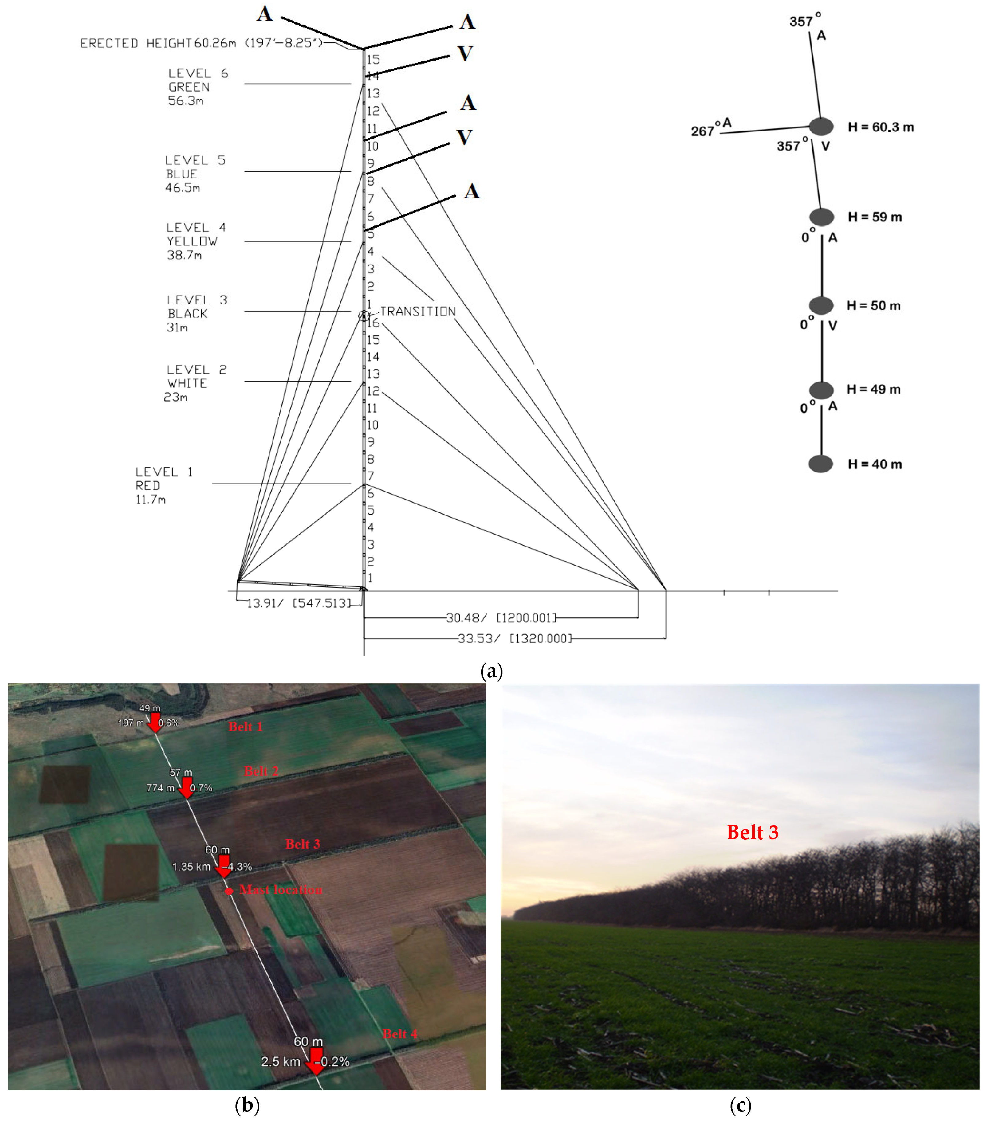
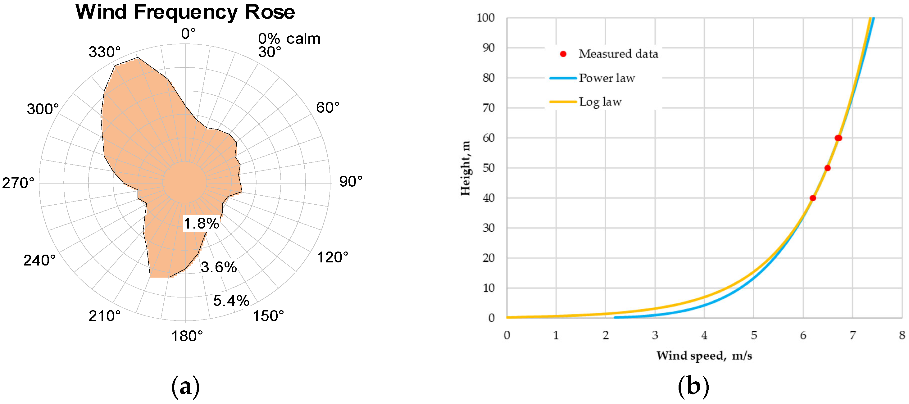
2.1. Experimental Setup

A 60 m meteorological mast with specialized instrumentation was used to evaluate the wind speed profile change with height. This mast was equipped with 3 calibrated anemometers that continuously measured the wind velocity and 2 wind vanes for wind direction. In addition, temperature and barometric pressure sensors were installed. They were fixed to heights of 40 m, 50 m, and 60 m, respectively [80] (Figure 1a). Ten-minute readings for the wind parameters were collected for more than one year, as the data were checked for consistency. To meet the wind potential measurement criteria, calibrated equipment was used [81]. The location of a measurement mast located immediately downstream southwards from belt 3 is presented in Figure 1b. A summary of the technical specifications of the measuring equipment used during the experiment is presented in

Table 1. Technical specifications of the measuring equipment.

Sensor	Type	Range	Precision
Anemometer	A100R	0.2 up to 75 m/s	1% of reading between 10 and 50 m/s, 2% above 50 m/s
Wind vane	200P	0 up to 360o	±3° steady winds over 5 m/s
Temperature	Vaisala HMP50	−40 up to 60 °C	±1.6 °C at −40 °C; up to ±0.4 °C at 0 °C; ±0.6 °C at 40 °C outdoor temperature
Humidity	Vaisala HMP50	0 to 100%	±3%

.

Based on the processed field data, the wind shear was reconstructed by fitting it to known mathematical relationships for the atmospheric wind profile. The mast was located downstream of a belt (Figure 1c), which can possibly disturb the profile near the ground. Since this disturbance is likely to be smaller at higher heights (as was confirmed by the results of the study), it was accepted that the measurement data from the mast, sampled at heights of 40–60 m, would not be affected significantly, so these data could be used to construct the atmospheric boundary layer profile. However, to acknowledge the fact that this profile will be disturbed near the ground if it is close behind a belt, the boundary condition was moved sufficiently downstream of the mast and a classical atmospheric boundary layer profile was assigned to it. The domain inlet was thus positioned around 1100 m downstream of the third belt and 176 m upstream of the fourth belt.

Studying the airflow above such a large area is a challenging task and can only be effectively accomplished numerically. Increasing numbers of field and model studies of the velocity and turbulence characteristics of the flow above land areas were performed recently [17]. In particular, the number of numerical studies has increased, among which RANS and Large-Eddy Simulations (LES) are the most popular choices. The present study was motivated by the need to define the value of the drag coefficient, respectively the momentum sink, within the tree belt region, as well as the value of turbulent viscosity, which largely determines the shape of the velocity profiles with height.

2.2. Numerical Method

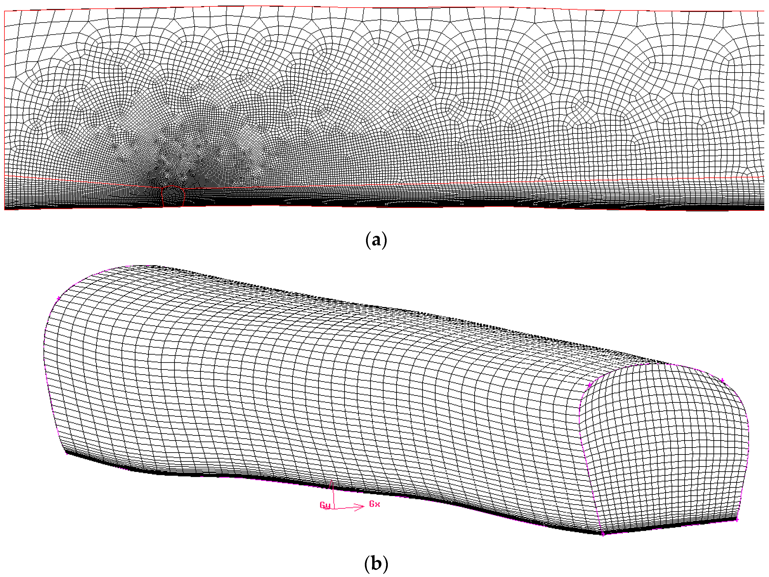
2.2.1. Computational Domain and Grid

To perform the numerical experiment, a proper geometric model of the studied terrain was required. The terrain topology has been prepared using both an online-based tool [82] and topographic maps (scale 1:5000 and 1:25,000). The data collected by [82] for the site in the vicinity of the mast were processed, and the surface area was prepared using the Kriging interpolation method [83] via Golden Software (TM)—Surfer, v15 (https://www.goldensoftware.com/products/surfer/, accessed on 27 June 2025).

The 3D model was compared to the one generated from the topographic map, showing a very good correlation. The resulting data were exported and imported into the Gambit mesh generator. The reference points were used to generate a surface, which was then extruded vertically to define the computational domain. This domain extended 176 m upstream and 2090 m downstream from the tree belt, with a vertical height of 220 m, sufficient to encompass typical wind turbine heights. The domain width was limited to 400 m and meshed with a coarse grid, as no significant velocity or turbulence gradients were expected in the spanwise direction.

The numerical grid in the streamwise direction can be seen in Figure 2a. Particular attention was given to accurately represent the geometry of the tree belt, as it constitutes a major momentum sink in the flow field. As seen in Figure 2b, its surface was made to mimic the natural form of forestry. Special attention was also paid to mesh refinement near the ground to satisfy the dimensionless y⁺ distance. Three grid meshes were constructed to study the grid sensitivity, and the mesh that satisfied the y⁺ values consisted of little more than 1.3 million cells. This was achieved with a streamlined boundary layer mesh that started with a cell height of 0.01 m over the ground and increased at a ratio of 1.2 for 20 cells upward. The numerical grid consisted entirely of hexahedral cells in a fully structured grid near the ground and pave-structured grid above the belt to allow for gradual coarsening. Considering the scale of the problem, this allowed for very economical mesh satisfying the numerical requirements of high-Re turbulence models.

2.2.2. Turbulence Modeling

Turbulence was modeled using the realizable k-ε turbulence model, selected due to its proven reliability in predicting flows characterized by separation, recirculation, and strong velocity gradients, conditions often encountered downstream of porous vegetation structures, such as tree belts. Compared to the standard k-ε model, the realizable variant employed modified formulations for turbulence viscosity, significantly improving accuracy in highly sheared and turbulent regions [84,85]. This model is widely validated and accepted in the literature for atmospheric boundary layer studies involving vegetation-induced momentum sinks [84].

To accurately capture the near-ground velocity and turbulence profiles specific to atmospheric flows, modified wall functions adapted for neutral atmospheric boundary layers were implemented. These atmospheric wall functions incorporate the aerodynamic roughness length (z₀), necessary for correctly modeling wind velocity profiles near surfaces with vegetation [86]. The parameters adopted were z₀ = 0.298 m and friction velocity u = 0.5 m/s, derived directly from the measured velocity data at the study site.

The turbulence kinetic energy (k) and turbulence dissipation rate (ε) were set at the inlet using logarithmic vertical profiles fitted to the experimental data, ensuring realistic turbulence intensity representation within the computational domain.

2.2.3. Boundary Conditions

The inflow to the domain was a turbulent atmospheric boundary layer. Its velocity profile can be approximated by a power law or a log-law function. Physical measurements of the wind direction (Figure 3a) revealed that the prevailing wind direction was north–northwest NNW (330°), with a secondary main direction at an azimuth of 200° south–southwest (SSW). The study presented results from the NNW wind direction, to which the tree belt was nearly perpendicular. For this wind direction, the power law and log-law profiles were used to fit the data from the measurement mast. The power law profile of velocity has the general appearance of [87]:

$${\displaystyle \frac{u}{u_{ref}}}={\left({\displaystyle \frac{z}{z_{ref}}}\right)}^{\alpha },$$

(1)

where α is the profile exponent and the ‘ref’ index refers to reference quantities for velocity and elevation. At a reference height of 40 m, the measured velocity was 6.2 m/s, which yielded a profile exponent of 0.196. According to [81], this profile exponent corresponded to a moderately rough (grass and farmland) to rough (park and vegetation) terrain. The migration from a farmland to a rough terrain can probably be explained by the presence of tree belts nearby.

The log-law profile has the general appearance:

$${\displaystyle \frac{u}{u_{\ast }}}={\displaystyle \frac{1}{\kappa }}ln\left({\displaystyle \frac{z+z_0}{z_0}}\right),$$

(2)

where:

• u_* = friction velocity (m/s),
• z₀ = aerodynamic terrain roughness (m).

Curve fitting with the three mast measurement points allowed to determine the friction velocity as $0.5 \mathrm{m}/\mathrm{s}$ and the aerodynamic terrain roughness as $z_0=0.298 \mathrm{m}$. This value also corresponds to a rough terrain. The log-law and power law curve-fitted profiles together with measured data are plotted in Figure 3b. The two analytical expressions yielded almost full agreement at elevations above the tree belt, which are of main interest for the operation of wind turbines. Therefore, any of the profiles could be used as a boundary condition for the simulation. However, the power law would predict an infinite velocity gradient at zero elevation; therefore, the log-wall expression was used as a boundary condition for velocity.

To determine the turbulent kinetic energy profile, the turbulent kinetic energy was first calculated at each measurement point from the formula:

$$k={\displaystyle \frac{3}{2}}{\left(U.I\right)}^2,$$

(3)

with $U$ and $I$ being the mean measured air velocity and turbulence intensity, respectively. Then, the log-law was applied to the turbulent kinetic energy in the form:

$$k={\displaystyle \frac{u_{\ast }^2}{\sqrt{C_{\mu }}}}\sqrt{C_{1}ln\left({\displaystyle \frac{z+z_0}{z_0}}\right)+C_2}.$$

(4)

The curve-fitting coefficients C₁ and C₂ defaulted to 0 and 1, respectively, which would result in a uniform value of k. However, calculations from measurements via Formula (5) indicated a slight variation in the value of k, and thus the coefficient C₁ was chosen as 0.22, while C₂ was retained as 1. This change proved to bring a negligible difference in the results. The same coefficient values were also used to assign the profile of the turbulent dissipation rate, given by:

$$\epsilon ={\displaystyle \frac{u_{\ast }^3}{\kappa (z+z_0)}}\sqrt{C_{1}ln\left({\displaystyle \frac{z+z_0}{z_0}}\right)+C_2}.$$

(5)

The high-Re turbulence model requires wall functions to set the boundary conditions at the wall, in this case the ground. Wall constraint was applied to the turbulent viscosity, the turbulent kinetic energy k, and its dissipation rate ε. As a first step, a standard wall function group was applied, in which the model expression for the turbulent viscosity is:

$${\nu }_t=f_{blend}\left({\nu }_{t\left(vis\right),}{\nu }_{t\left(log\right)}\right),$$

(6)

with

$$\begin{gathered} {\nu }_{t\left(vis\right)}=0 \\ {\nu }_{t\left(log\right)}={\nu }_w\left({\displaystyle \frac{y^{+}\kappa }{ln\left(E{y}^{+}\right)}}-1\right) \\ {y}^{+}=C_{\mu }^{1/4}y{\displaystyle \frac{\sqrt{k}}{{\nu }_w}}, \end{gathered}$$

(7)

where:

• ${\nu }_t=Turbulent viscosity \left[{\mathrm{m}}^2/\mathrm{s}\right]$
• ${\nu }_{t\left(vis\right)}={\nu }_t computed by viscous sublayer assumptions \left[{\mathrm{m}}^2/\mathrm{s}\right]$
• ${\nu }_{t\left(log\right)}={\nu }_t computed by inertial sublayer assumptions \left[{\mathrm{m}}^2/\mathrm{s}\right]$
• ${\nu }_w=Kinematic viscosity of fluid near wall \left[{\mathrm{m}}^2/\mathrm{s}\right]$
• $y^{+}=Estimated wall-normal height of the cell centre in wall units \left[-\right]$
• $\kappa =von Karman constant \left[-\right]$
• $E=wall roughness parameter \left[-\right]$
• $C_{\mu }=Emperical model constant \left[-\right]$
• $y=wall-normal height \left[\mathrm{m}\right]$
• $k=turbulent kinetic energy \left[{\mathrm{m}}^2/{\mathrm{s}}^2\right]$
• $f_{blend}=Wall-function blending operator$

The wall constraint on the turbulent kinetic energy was essentially a zero-gradient condition, which took care of the peculiarities of the k equation. The epsilon wall-boundary condition provided a wall constraint on the dissipation rate and on the turbulent kinetic energy production, G. Unlike the k wall function, in the epsilon wall function the value of the cell center, rather than the value on the cell face, is calculated, and the process involves stepwise blending between the viscous and inertial epsilon expressions depending on the y⁺ distance:

$${\epsilon }_{vis}=2\omega k{\displaystyle \frac{{\nu }_w}{y^2}},$$

(8)

$${\epsilon }_{log}=\omega C_{\mu }{\displaystyle \frac{k^{3/2}}{{\nu }_{tw}y}},$$

(9)

$$G=\omega \left({\nu }_{tw}+{\nu }_w\right)\left|n·{\left(\nabla u\right)}_f\right|C_{\mu }^{{\displaystyle \frac{1}{4}}}{\displaystyle \frac{k^{\frac{1}{2}}}{\kappa y}},$$

(10)

with ${\nu }_{tw}$ being the turbulent viscosity near the wall and $\omega$ the cell-corner weights. In the calculations, the stepwise blending was used, in which ${\epsilon =\epsilon }_{vis}$ if ${y^{+}<y}_{lam}^{+}$ and ${\epsilon =\epsilon }_{log}$ when ${y^{+}>y}_{lam}^{+}$, where $y_{lam}^{+}$ is the intersection of the viscous and inertial sublayers in wall units. With this set of wall functions, the finest mesh of this study produced y⁺ values in the range 49.5–94.5, with an average of 70. The first cell was thus very well positioned in the log layer.

After running the model in the absence of tree belt, it became clear, however, that these wall functions significantly overestimated the velocity profile in the lower heights (<h) compared to the atmospheric logarithmic profile. The reason behind this is, among other things, that these functions inherently lack the aerodynamic roughness height $z_0$ as a parameter, which is only relevant for atmospheric flows. For this reason, a specialized set of wall functions had to be deployed that handle atmospheric boundary layer conditions. The boundary condition for turbulent viscosity was thus modified based on the work of [86]:

$${\nu }_{t\left(w\right)}={\nu }_w\left({\displaystyle \frac{y^{+}\kappa }{ln\left(max\left(E^{\prime },1+{10}^{-4}\right)\right)}}-1\right),$$

(11)

with

$$u^{\ast }=C_{\mu }^{1/4}\sqrt{k},$$

(12)

$$y^{+}={\displaystyle \frac{u^{\ast }y}{{\nu }_w}},$$

(13)

$$E\prime ={\displaystyle \frac{y+z_0}{z_0}}.$$

(14)

In a similar way to the wall functions before, a wall constraint on the turbulent kinetic energy dissipation rate and on the turbulent kinetic energy production contribution was applied:

$$\epsilon ={\displaystyle \frac{\omega C_{\mu }^{3/4}{k}^{3/2}}{\kappa \left(y+z_0\right)}}.$$

(15)

with the new atmospheric boundary layer wall functions, the velocity profiles improved significantly, but the dimensionless wall distance y⁺ deteriorated to a value of 177 on average.

2.2.4. Modeling the Momentum Sink

The trees represent a momentum drag to the flow. This drag enters the momentum equations as a sink term introduced using the Darcy–Forchheimer law porosity model:

$$S=-\left(\mu d+f{\displaystyle \frac{\rho \left|U\right|}{2}}\right)\mathrm{U},$$

(16)

where $d$ is the Darcy coefficient (1/m²) and $f$ is the Forchheimer coefficient (1/m). The Darcy coefficient represents the viscous contribution, which for the studied flow was of secondary importance and was prescribed the value 1. The Forchheimer coefficient $f$ represents the porous drag, which for the present study was assigned values 0.1, 0.2, and 0.5 to simulate the effect of vegetation.

2.2.5. Discretization Schemes

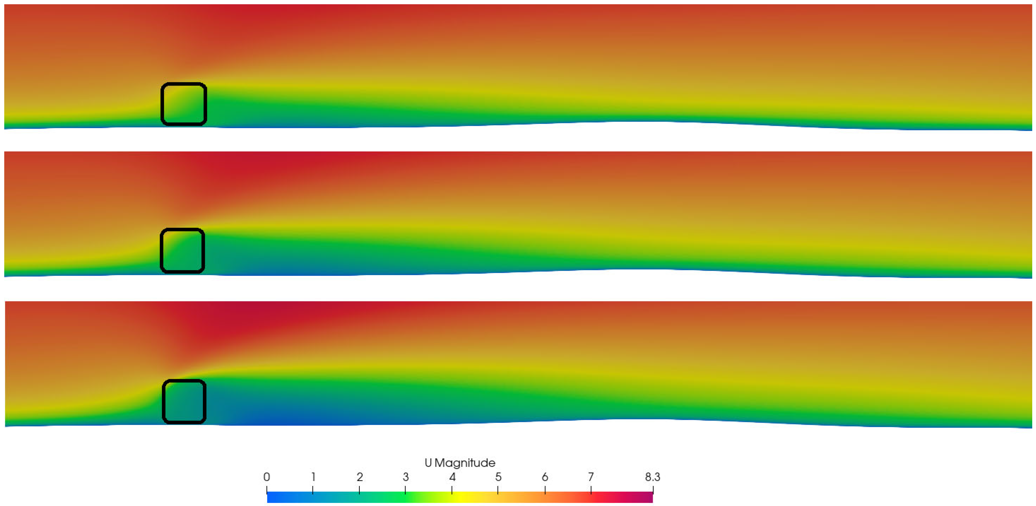
Different schemes were used for the terms in the transport equations of the velocity, k, and epsilon variables. The divergence and gradient terms are generally discretized by first applying the Gauss theorem and transforming the volume integral into a surface one. The face values have to be determined from the cell centers, which gives rise to different variants of interpolation schemes.

The gradient terms were discretized by Gauss and then face values were linearly determined from cell centers. The scheme, however, used a limiter that limited the gradient so that when extrapolating cell values to face values, the latter did not fall outside the bounds of values in surrounding cell centers.

The divergence terms are probably the most important and were treated accordingly for the equations for velocity, k, and epsilon. All used Gaussian integration, but the interpolation of cell to face values was different. For the velocity equation, the interpolation was upwind linear, which is second-order accurate and, at the same time, more limited by the linear interpolation scheme. For the divergence term of the scalar quantities k and epsilon, the cell to face interpolation was upwind, which is first-order accurate. All divergence schemes had the face value restricted within neighboring cells. All divergence schemes have, in addition, been bounded by including the divergence of velocity term in the calculations even though this term is zero in a converged solution of incompressible flow. A more detailed description of the schemes can be found in [88].

3. Results

The flow is influenced by the porous drag of the tree belt, but also by the skin friction with the ground. Wall functions play a vital role in determining the latter and its influence on the velocity profiles in the vertical direction. Standard wall functions were first attempted but they failed to predict the ground friction correctly under atmospheric flows. Figure 4 compares the predicted profiles of standard and atmospheric wall functions several hundred meters from the inlet in the absence of a tree belt. It is clear that the latter agreed practically completely with the logarithmic profile. There was some discrepancy in the lower heights, which can be attributed to the function model, or to the bit higher dimensionless wall distance, which rose from 70 to 170 on average after application of atmospheric wall functions. Yet this discrepancy, especially compared to standard wall functions, was marginal.

Three values of tree belt porosity were studied, giving rise to the velocity distributions in the central streamwise plane, as shown in Figure 5. The slow-down downstream of the belt became more clearly visible at porosity of 0.5 m⁻¹. The wake thickness increased and approached the size of wake behind a solid body. Thus, for porosity coefficients above 0.5–1 m⁻¹, little change is to be expected. It is worth mentioning that at higher-porosity drag, the flow above the belt accelerated in order to fulfill continuity. This can have implications for the operation of wind turbines in the immediate vicinity of the belt.

As the operation of wind turbines is also dependent on turbulence, the turbulent kinetic energy is presented in Figure 6 for the three porosity coefficients. The turbulence generation was mainly in the shear layer created by the belt, which was advected downstream. Here, the influence of belt porosity was clearly visible, both in the intensity and in the size of the influenced zone. For the low-porosity coefficient, the turbulent zone spanned around 1.5 tree belt heights in the vertical direction, and the increase in turbulence can be considered marginal. For the higher-porosity coefficient, the zone spanned around 2.5 tree heights, and the increase in turbulence was 2–3-fold compared to the flow upstream. The turbulence wake also increased in length, and for higher-porosity coefficients it may require a distance up to 15–20 tree heights (350–500 m) for the effect to practically dissolve.

In a next step, the vertical profiles of velocity at selected locations within the central streamwise plane were plotted for different porosity values. Figure 7 shows the case for the lowest porosity coefficient of 0.1 m⁻¹. The locations have been normalized with the height of the tree belt (h), with zero reference for the streamwise coordinate x taken at the front of the belt. As expected, the velocity behind the belt diminished, as demonstrated by the x = 2 h and x = 5 h profiles. However, the curves also showed that about 1.5 h above ground, the velocity started to increase, compared to the logarithmic atmospheric profile, and this increase gradually diminished until a height of about 150–200 m, where the velocity regained its logarithmic atmospheric layer value. Further downstream, this effect was less pronounced, but could be still witnessed until streamwise locations of 20–50 h. The reason is mass conservation, which increases the airflow above the belt to compensate for the obstructed flow through the belt. The higher the obstruction, the higher the effect on the velocity above the belt. Figure 8 shows the profiles for a porosity of 0.2 m⁻¹, which confirmed this hypothesis. The velocity deficit downstream of the belt was more pronounced and could be felt further downstream (x = 50 h). The velocity gain at elevations higher than 1.8–2 h was more pronounced, but this height depended more strongly on the streamwise location. Figure 9 shows profiles for the case with the highest porosity drag, and it is clear that the velocity deficit behind the belt was the strongest, and the gain above x = 2 h was even more pronounced, but with diminishing returns. It could be argued that for porosity coefficient bigger than 1, the results would be practically indistinguishable from a solid-body wake.

In all three cases, it could be observed that furthest downstream, the profiles did not completely recover to the logarithmic profile, although by a small margin. The tree belt, being an obstacle to the flow, tended to diminish the flow rate, but because of conservation, the flow rate escaped through the top of the domain. An integral calculation showed that 10% of the flow rate was lost through the domain top, i.e., around 90% of the flow rate was available for wind turbines behind the tree belt compared to the terrain upstream of the tree belt. The presence of an obstacle of that magnitude will inevitably push the velocity profile higher, with the overall effect of a lower gross flow rate behind the tree belt. This flow rate, though, as indicated, has the potential to concentrate in the area above the tree belt, giving a boost to a turbine performance at that location.

4. Discussion

This study revealed the complex interaction between tree belts and wind airflow, providing valuable guidance for agricultural and energy applications. The deviations in the velocity airfield induced by the tree belts extended significantly downstream. Vertical velocity profiles showed a key pattern: air velocity was lower below $z\approx 1.5 \mathrm{h}$ immediately downstream of the belt, while it increased above this height, $z>1.5 \mathrm{h}$, in a range of locations that depended on the belt porosity, ranging from $x=\left(1–4\right) \mathrm{h}$ to $x=\left(1 ÷ 50\right) \mathrm{h}$. This acceleration, as a result of the conservation-of-mass law, implies a compensation of the blocked airflow across the belt, which is consistent with the authors’ observations in [89] of similar compensatory effects in agricultural landscapes.

The increase in airflow velocity over the belt is consistent with the findings of the authors in [31], who reported air acceleration over porous vegetation barriers. However, the presented study is supplemented with a quantitative analysis, showing that placing turbines above $z>1.5 \mathrm{h}$ and near the belt can maximize their efficiency. However, care should be taken about excessive turbulence, which arises with higher-porosity drag coefficients. The total flow analysis revealed a 10% flow rate loss in the upper part of the domain, similar to the observations in [90], but also demonstrated that redistributed velocity over the belt concentrated the energy, which can improve the performance of the turbines.

In terms of turbulence, the study identified the shear layer up to 1.5 h as the main source of turbulence. In agreement with findings in [91], the present findings showed that drag coefficients around 0.5 m⁻¹ had a significant impact on the wake characteristics compared to lower-porosity drag, highlighting the differences in effects between porous and non-porous barriers.

The study showed that wind turbines located above $z>1.5 \mathrm{h}$ can benefit from the increased wind speed; however, to completely avoid induced turbulence effects near the belt, one may want to target elevations of 2.5 h and above. This recommendation builds on the work of the authors in [92], who stressed the importance of rotor positioning relative to turbulent zones. Also, reducing downstream turbulence implies less impact on turbines if they are located in these zones.

The relatively realistic belt geometry and physically correct boundary conditions, coupled with the robust model of porosity drag, provide a solid foundation for understanding the interactions between vegetation barriers and wind airflow. Future research can build on this approach by incorporating a diversity of vegetation types, even further seasonal variation (manifested by the porosity drag coefficient), and field validations to extend the applicability of results to real-world environments. In addition, integrating rotor dynamics and material fatigue models, as proposed in [93], will contribute to a more complete understanding of the long-term effects of turbulence on turbine durability and efficiency.

These findings are particularly relevant for rural energy planning and microgeneration systems. The observed flow acceleration above the tree belts and the turbulence patterns suggest that careful vertical positioning of wind turbines can lead to significant performance gains. In practice, placing turbines above the turbulence-affected zone (typically above 2.5 times the belt height) allows for better exploitation of the accelerated flow while minimizing structural loads caused by turbulent eddies. Moreover, the insensitivity of results beyond a porosity of 0.5 m⁻¹ indicates that extremely dense belts may not be cost-effective or necessary for aerodynamic optimization.

5. Conclusions

The study employed a realizable k–epsilon turbulence model to a large domain with porous drag. The inlet profiles of velocity, turbulent kinetic energy, and its dissipation rate were based on atmospheric research supplemented with measurement data. The terrain drag was modeled with two sets of wall functions, and it was proved that standard wall functions will not correctly predict atmospheric flows. This necessitated the use of atmospheric wall functions that resulted in very good agreement of the calculated velocity profiles with the theoretical logarithmic ones.

To summarize clearly the practical implications of this study: when placing small-scale wind turbines downstream of tree belts, it is advisable to position the turbine rotors at heights exceedingly approximately 2.5 times the height of the tree belt. This placement avoids substantial increases in turbulence intensity and benefits from the local acceleration in wind velocity above the tree belt. Additionally, choosing tree belt porosity coefficients beyond 0.5 m⁻¹ offers diminishing returns in modifying wind velocity and turbulence characteristics, suggesting that overly dense vegetation does not significantly enhance the protective or aerodynamic performance.

The requirements for dimensionless wall distance (y⁺) were met through significant mesh refinement near the ground, resulting in cell heights as small as 1 cm. The y⁺ increased after the application of atmospheric wall functions, but remained within reasonable limits, especially considering the size of the domain.

The belt represents an obstacle, and as such it tended to reduce the speed downstream. This decrease was compensated by a velocity increase starting at elevations 1.5 times the tree belt. The velocity deficit behind the belt and the corresponding gain at higher elevations were dependent on the belt porosity up to values of 0.5 m⁻¹. This effect is expected to diminish for further increases in porosity drag. The profiles furthest downstream of the belt never completely regained the undisturbed velocity profile, thus reducing, albeit marginally, the flow rate available for turbines.

The belt introduced substantial turbulent intensity for higher drag coefficients. The affected zone may reach a size of 2.5 tree heights in the vertical direction and a length of 15 tree heights downstream. This should be considered carefully during installation of wind turbines.

Future research will focus on extending the present methodology to more complex vegetation configurations, including heterogeneous tree belts with mixed porosity and height profiles. Experimental validation using wind tunnel measurements or LiDAR field data is also foreseen to strengthen the numerical findings and improve the parameterization of vegetation-induced drag in CFD models.

References

1. Kuntzman, J.; Brom, J. From Fields to Microclimate: Assessing the Influence of Agricultural Landscape Structure on Vegetation Cover and Local Climate in Central Europe. Remote Sens. 2025, 17, 6. [Google Scholar] [CrossRef]
2. Ntawuruhunga, D.; Ngowi, E.E.; Mangi, H.O.; Salanga, R.J.; Shikuku, K.M. Climate-smart agroforestry systems and practices: A systematic review of what works, what doesn’t work, and why. For. Policy Econ. 2023, 150, 102937. [Google Scholar] [CrossRef]
3. Mume, I.D.; Workalemahu, S. Review on Windbreaks Agroforestry as a Climate Smart Agriculture Practices. Am. J. Agric. For. 2021, 9, 342–347. [Google Scholar]
4. Ali, M.M.; Pal, A.C.; Bari, M.S.; Rahman, M.L.; Sarmin, I.J. Agroforestry as a Climate-Smart Strategy: Examining the Factors Affecting Farmers’ Adoption. Biol. Life Sci. Forum 2024, 30, 29. [Google Scholar]
5. Kanianska, R.; Kizeková, M.; Jančová, Ľ.; Čunderlík, J.; Dugátová, Z. Effect of Soil Erosion on Soil and Plant Properties with a Consequence on Related Ecosystem Services. Sustainability 2024, 16, 7037. [Google Scholar] [CrossRef]
6. Majaura, M.; Böhm, C.; Freese, D. The Influence of Trees on Crop Yields in Temperate Zone Alley Cropping Systems: A Review. Sustainability 2024, 16, 3301. [Google Scholar] [CrossRef]
7. Sadorsky, P. Wind energy for sustainable development: Driving factors and future outlook. J. Clean. Prod. 2021, 289, 125779. [Google Scholar] [CrossRef]
8. Kuczyński, W.; Wolniewicz, K.; Charun, H. Analysis of the wind turbine selection for the given wind conditions. Energies 2021, 14, 7740. [Google Scholar] [CrossRef]
9. Guo, X.; Zhang, X.; Du, S.; Li, C.; Siu, Y.L.; Rong, Y. The impact of onshore wind power pro-jects on ecological corridors and landscape connectivity in Shanxi, China. J. Clean. Prod. 2020, 254, 120075. [Google Scholar] [CrossRef]
10. Ali, S.; Taweekun, J.; Techato, K.; Waewsak, J.; Gyawali, S. GIS based site suitability assessment for wind and solar farms in Songkhla, Thailand. Renew. Energy 2019, 132, 1360–1372. [Google Scholar] [CrossRef]
11. Duranay, Z.B.; Güldemir, H.; Coşkun, B. The Role of Wind Turbine Siting in Achieving Sustainable Energy Goals. Processes 2024, 12, 2900. [Google Scholar] [CrossRef]
12. Cleugh, H.A. Field measurements of windbreak effects on airflow, turbulent exchanges and microclimates. Aust. J. Exp. Agric. 2002, 42, 665–677. [Google Scholar] [CrossRef]
13. Liu, X.; Zhao, T.; Pan, Y. Porous Barriers and Agricultural Wind Flow. Environ. Fluid Mech. 2020, 45, 34–56. [Google Scholar]
14. Zhou, Q.; Hu, T. Numerical Simulations of Wind Flow around Forest Belts. Environ. Fluid Mech. 2020, 45, 456–478. [Google Scholar]
15. Xie, S.; Martinez-Vazquez, P.; Baniotopoulos, C. Experimental Measurements of Wind Flow Characteristics on an Ellipsoidal Vertical Farm. Buildings 2024, 14, 3646. [Google Scholar] [CrossRef]
16. Pan, Y.; Liu, X.; Hu, T. LES Simulations for Wind Energy. J. Environ. Model. 2018, 56, 890–906. [Google Scholar]
17. Wang, J.; Patruno, L.; Zhao, G.; Tamura, Y. Windbreak effectiveness of shelterbelts with different characteristic parameters and arrangements by means of CFD simulation. Agric. For. Meteorol. 2024, 344, 109813. [Google Scholar] [CrossRef]
18. Hu, T.; Liu, X.; Zhao, P. Advanced Simulation Methods for Wind Shear Analysis. J. Fluid Dyn. 2021, 67, 245–260. [Google Scholar]
19. Wang, J.; Patruno, L.; Chen, Z.; Yang, Q.; Tamura, Y. Windbreak Effectiveness of Single and Double-Arranged Shelterbelts: A Parametric Study Using Large Eddy Simulation. Forests 2024, 15, 1760. [Google Scholar] [CrossRef]
20. Poulain, P.; Craig, K.J.; Meyer, J.P. Transient simulation of an atmospheric boundary layer flow past a heliostat using the Scale-Adaptive Simulation turbulence model. J. Wind. Eng. Ind. Aerodyn. 2021, 218, 104740. [Google Scholar] [CrossRef]
21. Szigeti, N.; Frank, N.; Vityi, A. The Multifunctional Role of Shelterbelts in Intensively Managed Agricultural Land—Silvoarable Agroforestry in Hungary. Acta Silv. Lignaria Hung. 2020, 16, 19–38. [Google Scholar] [CrossRef]
22. Abdalla, Y.Y.; Fangama, I.M. Effect of Shelterbelts on Crop Yield in the Agricultural Scheme of Al-Rahad, Sudan. Int. J. Curr. Microbiol. Appl. Sci. 2015, 4, 1–4. [Google Scholar]
23. Carnovale, D.; Bissett, A.; Thrall, P.H.; Baker, G. Plant genus (Acacia and Eucalyptus) alters soil microbial community structure and relative abundance in shelterbelts with regenerated vegetation. Appl. Soil Ecol. 2019, 133, 1–11. [Google Scholar] [CrossRef]
24. Zaady, E.; Katra, I.; Shuker, S.; Knoll, Y.; Shlomo, S. Tree Belts for Decreasing Aeolian Dust-Carried Pesticides from Cultivated Areas. Geosciences 2018, 8, 286. [Google Scholar] [CrossRef]
25. Zhang, L.; Wang, H.; Yu, C. Impact of Windbreaks on Airflow Dynamics. J. Renew. Energy Stud. 2019, 32, 123–136. [Google Scholar]
26. Siriri, D.; Wilson, J.; Coe, R.; Tenywa, M.M.; Bekunda, M.A.; Ong, C.K.; Black, C.R. Trees improve water storage and reduce soil evaporation in agroforestry systems on bench terraces in SW Uganda. Agrofor. Syst. 2013, 87, 45–58. [Google Scholar] [CrossRef]
27. Lin, B.B. The role of agroforestry in reducing water loss through soil evaporation and crop transpiration in coffee agroecosystems. Agric. For. Meteorol. 2010, 150, 510–518. [Google Scholar] [CrossRef]
28. Alharbi, S.; Felemban, A.; Abdelrahim, A.; Al-Dakhil, M. Agricultural and Technology-Based Strategies to Improve Water-Use Efficiency in Arid and Semiarid Areas. Water 2024, 16, 1842. [Google Scholar] [CrossRef]
29. Zhu, J.; Luo, X.; Zhai, Y.; Zhang, G.; Zhou, C.; Chen, Z. Study on the Impact of Tree Species on the Wind Environment in Tree Arrays Based on Fluid–Structure Interaction: A Case Study of Hangzhou Urban Area. Buildings 2024, 14, 1409. [Google Scholar] [CrossRef]
30. Zhang, L.; Zhan, Q.; Lan, Y. Effects of the tree distribution and species on outdoor environment conditions in a hot summer and cold winter zone: A case study in Wuhan residential quarters. Build. Environ. 2018, 130, 27–39. [Google Scholar] [CrossRef]
31. Manickathan, L.; Defraeye, T.; Allegrini, J.; Derome, D.; Carmeliet, J. Comparative study of flow field and drag coefficient of model and small natural trees in a wind tunnel. Urban For. Urban Green. 2018, 35, 230–239. [Google Scholar] [CrossRef]
32. Sun, Q.; Zheng, B.; Liu, T.; Zhu, L.; Hao, X.; Han, Z. The optimal spacing interval between principal shelterbelts of the farm-shelter forest network. Environ. Sci. Pollut. Res. 2022, 29, 12680–12693. [Google Scholar] [CrossRef]
33. Gualtieri, G.; Secci, S. Methods to extrapolate wind resource to the turbine hub height based on power law: A 1-h wind speed vs. Weibull distribution extrapolation comparison. Renew. Energy 2012, 43, 183–200. [Google Scholar] [CrossRef]
34. Wan, J.; Liu, J.; Ren, G.; Guo, Y.; Hao, W.; Yu, J.; Yu, D. A universal power-law model for wind speed uncertainty. Clust. Comput. 2019, 22, 10347–10359. [Google Scholar] [CrossRef]
35. Liu, H.; Chen, G.; Hua, Z.; Zhang, J.; Wang, Q. Wind Shear Model Considering Atmospheric Stability to Improve Accuracy of Wind Resource Assessment. Processes 2024, 12, 954. [Google Scholar] [CrossRef]
36. Zhou, L.; Wu, H.; Li, Z.N. Review of research on trees’ wind resistance and effects on wind environment. J. Nat. Disasters 2015, 24, 199–206. [Google Scholar]
37. Wu, X.; Zou, X.; Zhou, N.; Zhang, C.; Shi, S. Deceleration efficiencies of shrub windbreaks in a wind tunnel. Aeolian Res. 2015, 16, 11–23. [Google Scholar] [CrossRef]
38. Zeng, F.; Simeja, D.; Ren, X.; Chen, Z.; Zhao, H. Influence of Urban Road Green Belts on Pedestrian-Level Wind in Height-Asymmetric Street Canyons. Atmosphere 2022, 13, 1285. [Google Scholar] [CrossRef]
39. Chan, P.W.; Lai, K.K. Evidence of Terrain-Induced Windshear Due to Lantau Island over the Third Runway of the Hong Kong International Airport—Examples and Numerical Simulations. Appl. Sci. 2025, 15, 83. [Google Scholar] [CrossRef]
40. Zhou, X.H.; Brandle, J.R.; Mize, C.W.; Takle, E.S. Three-dimensional aerodynamic structure of a tree shelterbelt: Definition, characterization and working models. Agrofor. Syst. 2005, 63, 133–147. [Google Scholar] [CrossRef]
41. Ren, X.; Zhang, G.; Chen, Z.; Zhu, J. The Influence of Wind-Induced Response in Urban Trees on the Surrounding Flow Field. Atmosphere 2023, 14, 1010. [Google Scholar] [CrossRef]
42. Lee, S.-H.; Kim, H.; Moon, H.; Kim, H.-S.; Han, S.-S.; Jeong, S. Effects of Wind Barrier Porosity and Inclination on Wind Speed Reduction. Appl. Sci. 2023, 13, 8310. [Google Scholar] [CrossRef]
43. Wu, X.; Guo, Z.; Wang, R.; Fan, P.; Xiang, H.; Zuo, X.; Yin, J.; Fang, H. Optimal design for wind fence based on 3D numerical simulation. Agric. For. Meteorol. 2022, 323, 109072. [Google Scholar] [CrossRef]
44. Zhao, Z.; Tang, L.; Xiao, Y. Simulation of the Neutral Atmospheric Flow Using Multiscale Modeling: Comparative Studies for SimpleFoam and Fluent Solver. Atmosphere 2024, 15, 1259. [Google Scholar] [CrossRef]
45. Sharma, A.; Brazell, M.J.; Vijayakumar, G.; Ananthan, S.; Cheung, L.; deVelder, N.; Henry de Frahan, M.T.; Matula, N.; Mullowney, P.; Rood, J.; et al. ExaWind: Open-source CFD for hybrid-RANS/LES geometry-resolved wind turbine simulations in atmospheric flows. Wind Energy 2024, 27, 225–257. [Google Scholar] [CrossRef]
46. Misar, A.S.; Uddin, M. Effects of Solver Parameters and Boundary Conditions on RANS CFD Flow Predictions over a Gen-6 NASCAR Racecar; SAE Technical Papers; SAE International: Warrendale, PA, USA, 2022. [Google Scholar]
47. Siddiqui, M.S.; Khalid, M.H.; Zahoor, R.; Butt, F.S.; Saeed, M.; Badar, A.W. A numerical investigation to analyze effect of turbulence and ground clearance on the performance of a roof top vertical–axis wind turbine. Renew. Energy 2021, 164, 978–989. [Google Scholar] [CrossRef]
48. Lu, S.; Liu, J.; Hekkenberg, R. Mesh properties for RANS simulations of airfoil-shaped profiles: A case study of rudder hydrodynamics. J. Mar. Sci. Eng. 2021, 9, 1062. [Google Scholar] [CrossRef]
49. Ma, G.; Tian, L.; Song, Y.; Zhao, N. Effects of Turbulence Modeling on the Simulation of Wind Flow over Typical Complex Terrains. Appl. Sci. 2024, 14, 11438. [Google Scholar] [CrossRef]
50. Drame, A.S.; Wang, L.; Zhang, Y. Granular Stack Density’s Influence on Homogeneous Fluidization Regime: Numerical Study Based on EDEM-CFD Coupling. Appl. Sci. 2021, 11, 8696. [Google Scholar] [CrossRef]
51. Tan, X.; Liu, Y.; Sha, B.; Zhang, N.; Chen, J.; Wang, H.; Mao, J. Study on Wind Resistance Performance of Transmission Tower Using Fixture-Type Reinforcement Device. Appl. Sci. 2025, 15, 747. [Google Scholar] [CrossRef]
52. Chougule, A.; Mann, J.; Segalini, A.; Dellwik, E. Spectral tensor parameters for wind turbine load modeling from forested and agricultural landscapes. Wind Energy 2015, 18, 469–481. [Google Scholar] [CrossRef]
53. He, C.; Shao, W. Numerical simulation of shelter effect assessment for single-row windbreaks on the periphery of oasis farmland. J. Arid. Environ. 2024, 222, 105165. [Google Scholar] [CrossRef]
54. Aili, A.; Xu, H.; Waheed, A.; Bakayisire, F.; Xie, Y. Synergistic windbreak efficiency of desert vegetation and oasis shelter forests. PLoS ONE 2024, 19, e0312876. [Google Scholar] [CrossRef]
55. Guo, Z.; Yang, X.; Wu, X.; Zou, X.; Zhang, C.; Fang, H.; Xiang, H. Optimal design for vegetative windbreaks using 3D numerical simulations. Agric. For. Meteorol. 2021, 298–299, 108290. [Google Scholar] [CrossRef]
56. Dimitrov, N.; Natarajan, A.; Kelly, M.C. Model of wind shear conditional on turbulence and its impact on wind turbine loads. Wind Energy 2015, 18, 1917–1931. [Google Scholar] [CrossRef]
57. Ren, G.; Liu, J.; Wan, J.; Li, F.; Guo, Y.; Yu, D. The analysis of turbulence intensity based on wind speed data in onshore wind farms. Renew. Energy 2018, 123, 756–766. [Google Scholar] [CrossRef]
58. Zhao, X.; Jiang, N.; Liu, J.; Yu, D.; Chang, J. Short-term average wind speed and turbulent standard deviation forecasts based on one-dimensional convolutional neural network and the integrate method for probabilistic framework. Energy Convers. Manag. 2020, 203, 112239. [Google Scholar] [CrossRef]
59. Zhu, C.; Yang, Q.; Wang, D.; Huang, G.; Liang, S. Fragility Analysis of Transmission Towers Subjected to Downburst Winds. Appl. Sci. 2023, 13, 9167. [Google Scholar] [CrossRef]
60. Dimitrov, N.; Natarajan, A.; Mann, J. Effects of normal and extreme turbulence spectral parameters on wind turbine loads. Renew. Energy 2017, 101, 1180–1193. [Google Scholar] [CrossRef]
61. Cheng, S.; Elgendi, M.; Lu, F.; Chamorro, L.P. On the Wind Turbine Wake and Forest Terrain Interaction. Energies 2021, 14, 7204. [Google Scholar] [CrossRef]
62. Badrkhani Ajaei, B.; El Naggar, M.H. Consideration of Rocking Wind Turbine Foundations on Undrained Clay with an Efficient Constitutive Model. Appl. Sci. 2025, 15, 457. [Google Scholar] [CrossRef]
63. Shen, S.; Zhang, H.; Li, F.; Chen, W. Optimizing wind turbine placement in agricultural areas with tree belts: A study on flow acceleration and maintenance cost reduction. Renew. Energy 2021, 175, 920–930. [Google Scholar]
64. Hernandez-Ramirez, G.; Hatfield, J.L.; Prueger, J.H.; Sauer, T.J. Energy balance and turbulent flux partitioning in a corn-soybean rotation in the Midwest US. Theor. Appl. Climatol. 2010, 100, 79–92. [Google Scholar] [CrossRef]
65. Vanderwende, B.; Lundquist, J.K. Could crop height affect the wind resource at agriculturally productive wind farm sites? Bound.-Layer Meteorol. 2016, 158, 409–428. [Google Scholar] [CrossRef]
66. Li, L.; Ma, W.; Duan, X.; Wang, S.; Wang, Q.; Gu, H.; Wang, J. Effects of Wind Farm Construction on Soil Nutrients and Vegetation: A Case Study of Linxiang Wind Farm in Hunan Province. Sustainability 2024, 16, 6350. [Google Scholar] [CrossRef]
67. Han, X.; Lu, C.; Wang, J. Long-Term Impacts of 250 Wind Farms on Surface Temperature and Vegetation in China: A Remote Sensing Analysis. Remote Sens. 2025, 17, 10. [Google Scholar] [CrossRef]
68. Chen, X.; Ye, X.; Zhang, Y.; Xiong, X. Analysis of Wind Speed Characteristics Along a High-Speed Railway. Appl. Sci. 2025, 15, 138. [Google Scholar] [CrossRef]
69. Bošnjaković, M.; Hrkać, F.; Stoić, M.; Hradovi, I. Environmental Impact of Wind Farms. Environments 2024, 11, 257. [Google Scholar] [CrossRef]
70. Jia, Z.; Yang, X.; Chen, A.; Yang, D.; Zhang, M.; Wei, L. Localized Eco-Climatic Impacts of Onshore Wind Farms: A Review. J. Resour. Ecol. 2024, 15, 151–160. [Google Scholar]
71. Miri, A.; Webb, N.P. Characterizing the spatial variations of wind velocity and turbulence intensity around a single Tamarix tree. Geomorphology 2022, 414, 108382. [Google Scholar] [CrossRef]
72. Cleugh, H.A. Effects of windbreaks on airflow, microclimates and crop yields. Agrofor. Syst. 1998, 41, 55–84. [Google Scholar] [CrossRef]
73. Li, Y.; Li, Z.; Chang, S.X.; Cui, S.; Jagadamma, S.; Zhang, Q.; Cai, Y. Residue retention promotes soil carbon accumulation in minimum tillage systems: Implications for conservation agriculture. Sci. Total. Environ. 2020, 740, 140147. [Google Scholar] [CrossRef] [PubMed]
74. Sun, W.; Canadell, J.G.; Yu, L.; Yu, L.; Zhang, W.; Smith, P.; Fischer, T.; Huang, Y. Climate drives global soil carbon sequestration and crop yield changes under conservation agriculture. Glob. Change Biol. 2020, 26, 3325–3335. [Google Scholar] [CrossRef] [PubMed]
75. Wang, Y.; Zeng, X.; Decker, J.; Dawson, L. A GPU-Implemented Lattice Boltzmann Model for Large Eddy Simulation of Turbulent Flows in and around Forest Shelterbelts. Atmosphere 2024, 15, 735. [Google Scholar] [CrossRef]
76. Huang, Y.; Zheng, M.; Li, T.; Xiao, F.; Zheng, X. An Integrated Framework for Landscape Indices’ Calculation with Raster–Vector Integration and Its Application Based on QGIS. ISPRS Int. J. Geo-Inf. 2024, 13, 242. [Google Scholar] [CrossRef]
77. Shin, S.S.; Park, S.D.; Kim, G. Applicability Comparison of GIS-Based RUSLE and SEMMA for Risk Assessment of Soil Erosion in Wildfire Watersheds. Remote Sens. 2024, 16, 932. [Google Scholar] [CrossRef]
78. Li, H.; Yan, Z.; Zhang, Z.; Lang, J.; Wang, X. A Numerical Study of the Effect of Vegetative Windbreak on Wind Erosion over Complex Terrain. Forests 2022, 13, 1072. [Google Scholar] [CrossRef]
79. Kong, T.; Liu, B.; Henderson, M.; Zhou, W.; Su, Y.; Wang, S.; Wang, L.; Wang, G. Effects of Shelterbelt Transformation on Soil Aggregates Characterization and Erodibility in China Black Soil Farmland. Agriculture 2022, 12, 1917. [Google Scholar] [CrossRef]
80. Terziev, A.; Panteleev, Y.; Iliev, I.; Beloev, H. Evaluation of the influence of the windbreak trees on the change of wind shear in weakly complex terrains. E3S Web Conf. 2021, 286, 02015. [Google Scholar] [CrossRef]
81. Available online: https://www.vde-verlag.de/iec-normen/251347/iec-61400-50-1-2022.html (accessed on 6 January 2025).
82. Available online: http://www.dataforwind.com/ (accessed on 6 January 2025).
83. Cressie, N.A.C. The Origins of Kriging. Math. Geol. 1990, 22, 239–252. [Google Scholar] [CrossRef]
84. Gromke, C.; Blocken, B. Influence of avenue-trees on air quality at the urban neighborhood scale. Part I: Quality assurance studies and turbulent Schmidt number analysis for RANS CFD simulations. Environ. Pollut. 2015, 196, 214–223. [Google Scholar] [CrossRef]
85. Blocken, B.; Stathopoulos, T.; Carmeliet, J. CFD simulation of the atmospheric boundary layer: Wall function problems. Atmos. Environ. 2007, 41, 238–252. [Google Scholar] [CrossRef]
86. Hargreaves, D.M.; Wright, N.G. On the use of the k–ε model in commercial cfd software to model the neutral atmospheric boundary layer. J. Wind Eng. Ind. Aerodyn. 2007, 95, 355–369. [Google Scholar] [CrossRef]
87. Hellman, G. Über die Bewegung der Luft in den untersten Schichten der Atmosphäre. Meteorol. Z. 1915, 32, 273–285. [Google Scholar]
88. Greenshields, C.J.; Weller, H.G. Weller Notes on Computational Fluid Dynamics: General Principles ISBN-10 1399920782. Available online: https://doc.cfd.direct/notes/cfd-general-principles/numerical-method (accessed on 6 January 2025).
89. Bergstrom, D.J.; Kotey, N.A.; Tachie, M.F. The Effects of Surface Roughness on the Mean Velocity Profile in a Turbulent Boundary Layer. J. Fluids Eng. 2002, 124, 664–670. [Google Scholar] [CrossRef]
90. Carlo, O.S.; Fellini, S.; Palusci, O.; Marro, M.; Salizzoni, P.; Buccolieri, R. Influence of Obstacles on Urban Canyon Ventilation and Air Pollutant Concentration: An Experimental Assessment. Build. Environ. 2024, 250, 111143. [Google Scholar] [CrossRef]
91. Arunvinthan, S.; Gouri, P.; Divysha, S.; Devadharshini, R.; Nithya Sree, R. Effect of Trough Incidence Angle on the Aerodynamic Characteristics of a Biomimetic Leading-Edge Protuberanced (LEP) Wing at Various Turbulence Intensities. Biomimetics 2024, 9, 354. [Google Scholar] [CrossRef]
92. Tucker, P.G. Trends in Turbomachinery Turbulence Treatments. Progress. Aerosp. Sci. 2013, 63, 1–32. [Google Scholar] [CrossRef]
93. Schwarz, C.M.; Ehrich, S.; Peinke, J. Wind turbine load dynamics in the context of turbulence intermittency. Wind Energy Sci. 2019, 4, 581–594. [Google Scholar] [CrossRef]
Figure 1. (a) Mast and sensor diagram, (b) satellite image of the surveyed area with location, distance, and elevation of the three belts, and (c) field photo of belt 3.
Applsci 15 07450 g001
Figure 2. (a) Numerical mesh of the streamwise plane. (b) Tree belt mesh.
Applsci 15 07450 g002
Figure 3. (a) Prevailing wind direction at 40 m height based on on-site data, (b) Log-law and power law profiles fitted to experimental data.
Applsci 15 07450 g003
Figure 4. Comparison of standard and atmospheric wall functions.
Applsci 15 07450 g004
Figure 5. Velocity (m/s) contours in the central streamwise plane with belt porosity coefficients of 0.1 m−1 (top), 0.2 m−1 (middle), and 0.5 m−1 (bottom).
Applsci 15 07450 g005
Figure 6. Turbulent kinetic energy (m2/s2) contours in the central streamwise plane with belt porosity coefficients of 0.1 m−1 (top), 0.2 m−1 (middle), and 0.5 m−1 (bottom).
Applsci 15 07450 g006
Figure 7. Velocity profiles at locations normalized with the tree belt height for the porosity coefficient 0.1 m−1.
Applsci 15 07450 g007
Figure 8. Velocity profiles at locations normalized with the tree belt height for the porosity coefficient 0.2 m−1.
Applsci 15 07450 g008
Figure 9. Velocity profiles at locations normalized with the tree belt height for the porosity coefficient 0.5 m−1.
Applsci 15 07450 g009