Progressive Landslide Prediction Using an Inverse Velocity Method with Multiple Monitoring Points of Synthetic Aperture Radar

Abstract

Accurate landslide time prediction holds critical significance for ensuring safety and efficient production in open-pit mining operations. While the inverse velocity method serves as a prevalent data-driven forecasting approach, conventional single-point monitoring implementations frequently yield substantial deviations. This study proposes a multi-point collaborative inverse velocity landslide time prediction methodology using nonlinear least squares, which is based on slope radar multi-point group displacement monitoring data. Systematic stability evaluations were conducted for both single-point predictions and multi-point ensemble forecasts. Experimental results demonstrate that single-point-based predictions generally confine errors within 5 h, including the case of traditional smoothing treatments of velocity curves. The developed multi-point collaborative methodology achieves prediction errors below 1 h, with temporal forecast position variations and spatial point quantity adjustments inducing marginal error fluctuations under 2 h based on strict data exclusion. Enhanced data volume implementation significantly improves prediction accuracy and stability. These findings will provide substantive technical references and methodological guidance for advancing landslide temporal prediction research in open-pit mining engineering.

1. Introduction

Landslides constitute a predominant geological hazard in open-pit mines. Approximately 80% of major disasters documented in the past two decades were attributed to landslides, underscoring the critical need for advanced landslide prediction research [1]. Among diverse landslide prediction methodologies, the inverse velocity method (INV), pioneered by Fukuzono [2], has gained prominence due to its conceptual simplicity and robust applicability in time-prediction scenarios [3,4,5]. This method derives predicted failure times by extrapolating the intersection of fitting inverse velocity and time curves during the accelerated creep phase of slopes.

Petley et al. [6] examined the movement histories of a number of landslides that occurred in a variety of materials in a range of settings and demonstrated that the evaluation of plots of inverse velocity against time for landslides is a useful technique for forecasting movement styles and rates, and for interpreting ongoing deformation processes in real time. Rose et al. [7] conducted comparative case studies to systematically evaluate the INV’s advantages and limitations, particularly emphasizing its efficacy in imminent landslide prediction. Dick et al. [8] applied the INV to radar displacement monitoring of open-pit mine slopes and suggested linear time prediction should be performed if a trend update point appears. Wang et al. [9] demonstrated through rheological experiments that INV parameters exhibit remarkable stability under varying loads and moisture conditions. Iwata et al. [10] enhanced prediction accuracy by selectively utilizing deformation acceleration data for INV calculations. Qi et al. [11] proposed a method for landslide prediction by combining three parameters—extent of change (EOC), extent of stability (EOS), and extent of mutation (EOM)—with the inverse velocity method, and the effectiveness of the method was verified by the measured data of a landslide in Yunnan Province, China. Zhang et al. [12] divided the landslide time uncertainty into observation uncertainty and model uncertainty and constructed a landslide time forecast method based on the principle of probability. Ma et al. [13] developed a dynamic accelerated point identification method using normal distribution confidence intervals, establishing a logarithmic time-prediction model. Recent studies by Du et al. [14] and Tao et al. [5] systematically investigated filtering algorithms’ impacts on INV performance, while Sharifi et al. [15] conducted a comparative examination of the INV and three other methods on a comprehensive database of 75 historical landslides.

The above studies all indicate that the INV can obtain relatively accurate prediction results but does not emphasize the spatial position of the point used relative to the landslide body, which means that the displacement velocity data of all points within the landslide body can be considered for landslide time prediction. A key point addressed in this work is improving the accuracy and stability of landslide time prediction through the advanced utilization of displacement velocity measurements obtained from multiple monitoring points. This study proposes a multi-point collaborative inverse velocity landslide time prediction methodology for the case of α = 2 using nonlinear least squares, which is based on slope radar multi-point group displacement monitoring data. The effectiveness and robustness of the proposed method are tested by comparing the results with those of single-point prediction and using different numbers of point clusters. It is hoped that this method can provide some reference for landslide time prediction in open-pit mines.

2. Materials and Methods

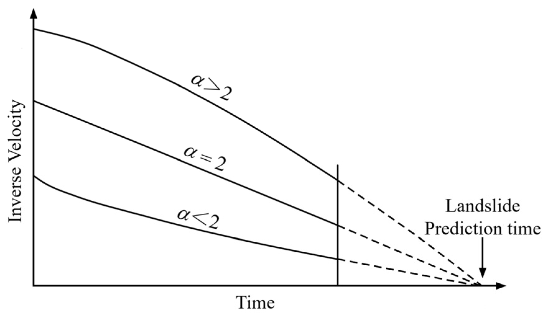
2.1. Principles of the Inverse Velocity Method (INV)

Under constant load conditions, the inverse deformation velocity (1/v or Λ) can be described by the following equation [2]:

$${\displaystyle \frac{1}{V}}={\left[A\left(\alpha -1\right)\right]}^{{\displaystyle \frac{1}{\alpha -1}}}{\left(t_f-t\right)}^{{\displaystyle \frac{1}{\alpha -1}}}$$

(1)

where V represents deformation velocity, t denotes time, t_f corresponds to predicted failure time, and A and α are material-specific constants. Following Voight’s [16,17] empirical validation, the exponent α typically assumes a value of 2 for geological materials, which yields the simplified formulation:

$${\displaystyle \frac{1}{V}}=A\left(t_f-t\right)$$

(2)

Equation (2) serves as the foundational predictive formula of the inverse velocity method for landslide time prediction, which is used in this study. The operational workflow is summarized in Figure 1.

2.2. Principle of Nonlinear Least Squares

The traditional calculation of the INV (α = 2) is generally based on the linear least squares method. However, when fitting the unified forecast time based on multi-point data at the same time, it is necessary to achieve a good linear fitting effect for each point and minimize the sum of fitting errors for all points, that is, the nonlinear least squares method should be used.

The goal of the nonlinear least squares problem is to find a parameter t such that the sum of squared residuals is minimized:

$$\underset{t}{\mathit{min}}{‖f\left(t\right)‖}_2^2=\underset{t}{\mathit{min}}\left(f_1{\left(t\right)}^2+f_2{\left(t\right)}^2+\cdots +f_n{\left(t\right)}^2\right)$$

(3)

Among them, $f_1{\left(t\right)}^2$ is the sum of squared least squares residuals of point 1, that is, the difference between the fitted line and the time series point, and the other numbers are similar; finally, the sum of squared residuals needs to be minimized. This method combines the advantages of the Gaussian Newton method and the Gradient Descent method to achieve fast convergence while ensuring stability. The real-time implementation of this method can be realized by using the lsqnonlin function of the MATLAB R2023b platform.

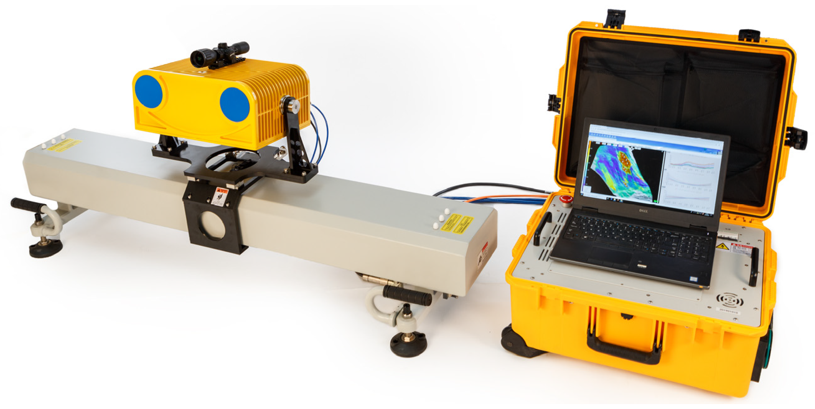
2.3. Principles of Slope Radar Monitoring

S-SAR (Slope Synthetic Aperture Radar), a ground deformation monitoring system based on microwave remote sensing technology, achieves millimeter-level displacement measurement accuracy through the emission of electromagnetic waves and the reception of reflected signals from target areas (Figure 2). Integrating Synthetic Aperture Radar (SAR) imaging with Differential Interferometric Synthetic Aperture Radar (DInSAR) principles, this system demonstrates technical advantages including all-weather operation, non-contact measurement, and large-area continuous monitoring. It has become an essential monitoring solution for mine slopes and geological hazard prevention [18,19,20].

During the operation of S-SAR, the radar continuously emits Frequency-Modulated Continuous Wave (FMCW) signals characterized by linear frequency variation over time. The echo signals from targets at different distances exhibit frequency differences due to time delays. Through quadrature demodulation of the received scattered echoes, these frequency differences are converted into time differences, thereby achieving high range resolution R₀. The calculation formula is as follows:

$$R_0={\displaystyle \frac{c}{2B}}$$

(4)

where c is the electromagnetic wave propagation velocity, and B represents the signal bandwidth.

For azimuth resolution, when the radar antenna moves along the azimuth direction, the relative motion between the radar and targets at different azimuth positions generates Doppler frequency shifts. By recording and processing the echo signals from each target, the system distinguishes azimuth targets based on these Doppler frequency variations, thereby enhancing azimuth resolution. Ultimately, the fusion of range and azimuth information synthesizes a two-dimensional radar image. The azimuth resolution P₀ is calculated as:

$$P_0={\displaystyle \frac{\lambda }{2L}}$$

(5)

where λ is wavelength, and L denotes the synthetic aperture length of the radar.

The deformation monitoring capability of S-SAR is based on differential interferometry. By performing coherent processing on the complex images acquired from two sequential measurements, the system extracts phase difference information. The phase difference is calculated using the following formula [21]:

$$\mathsf{\Delta }\varphi ={\displaystyle \frac{4\pi }{\lambda }}R+{\varphi }_{\mathrm{atm}1}+{\varphi }_{topo1}+{\varphi }_{noise1}$$

(6)

where $\mathsf{\Delta }\varphi$ is the Interferometric phase difference; R is the Line-of-sight (LOS) displacement; ${\varphi }_{\mathrm{atm}1}$ is the Atmospheric delay phase; ${\varphi }_{topo1}$ is the Topographic phase; and ${\varphi }_{noise1}$ is the Noise phase.

The topographic phase is eliminated through differential interferometric processing, while atmospheric phase correction is applied to mitigate the effects of atmospheric delay. Finally, LOS deformation inversion is performed. For slope monitoring scenarios, the deformation gradient is typically assumed to vary linearly within the pixel range. The least squares method is employed to unwrap discrete phase data, combined with precision calibration parameters, to achieve millimeter-level deformation monitoring accuracy. The deformation magnitude is calculated as follows:

$$R={\displaystyle \frac{\lambda }{4\pi }}·\mathsf{\Delta }\mathsf{\varphi }$$

(7)

The specific technical parameters of S-SAR are shown in

Table 1. S-SAR Technical Parameters.

Technical Parameters and Units	Numerical Value
Usage frequency (GHz)	17~18
Monitoring accuracy (mm)	0.1
Distance resolution (m)	0.15~0.3
Azimuthal resolution (mrad)	4~10
Collection frequency (min)	1–10

.

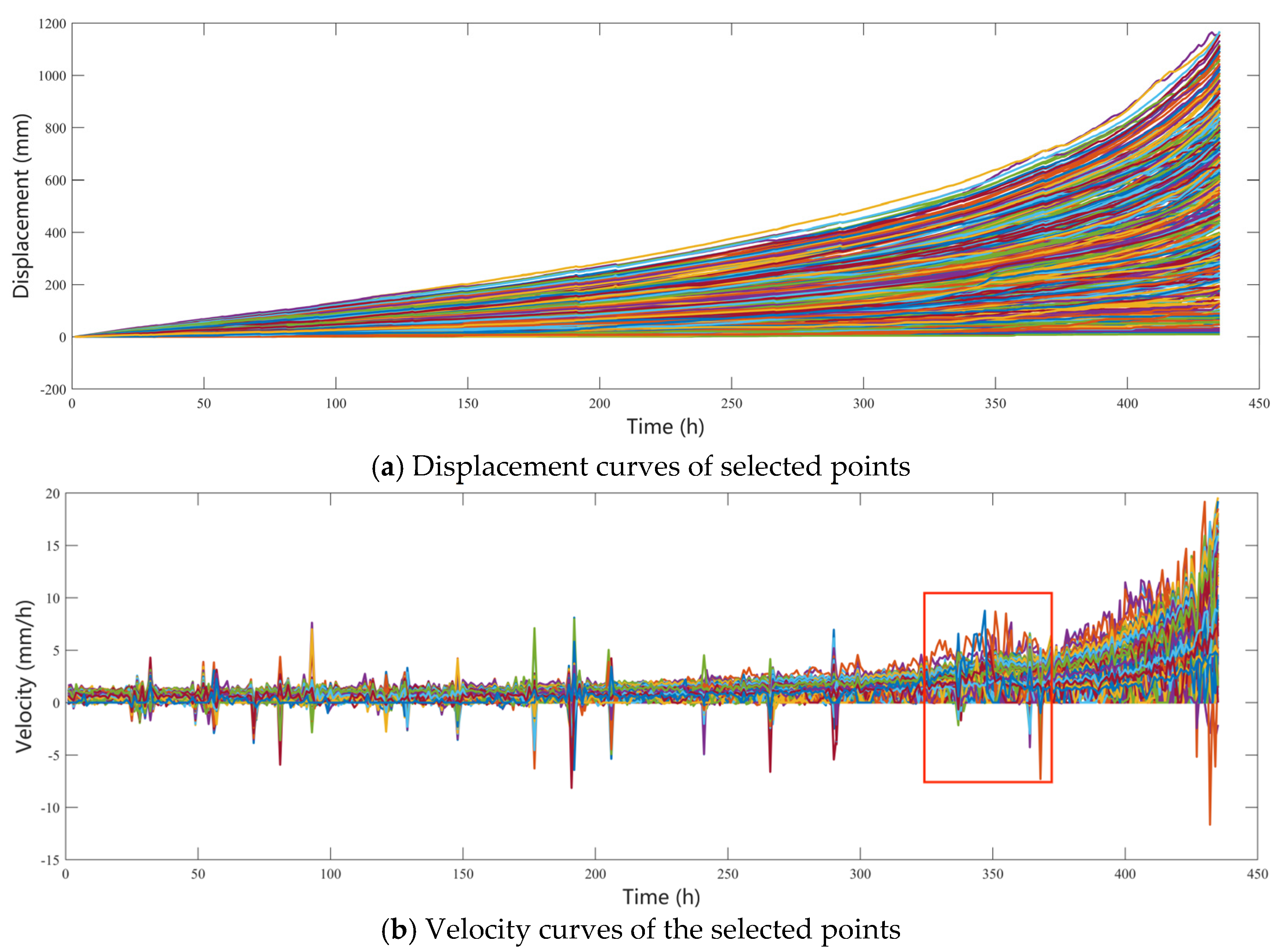
3. Mine Overview and Monitoring Data

A large open-pit copper-cobalt mine overseas has experienced slope failures of varying magnitudes across multiple locations in its mining area as excavation progressed to deeper levels. To ensure operational safety, the S-SAR system was deployed in August 2024 to monitor the deformation of slope. Continuous deformation was observed following the initiation of radar monitoring, culminating in a large-scale collapse at 1:00 AM on August 27, affecting seven benches and covering an area exceeding 10,000 square meters. Due to the timely and accurate warnings provided by the S-SAR system, the incident resulted in zero casualties and no property damage. The monitoring data collected by the S-SAR system (August 8 to August 27) and the characteristics of the landslide are presented in Figure 3. The landslide area is primarily composed of silty clay, argillaceous siltstone, argillaceous sandstone, conglomerate, and dolomite with serpentinization. The rock and soil strata are predominantly characterized by an adverse dip structure, with the rock mass quality classified as Grade V, exhibiting well-developed discontinuities/joints. Due to the lack of rainfall in the mining area during the monitoring period of the study, the impact of rainfall on the landslide process is not considered.

To facilitate systematic investigation and analysis, 120 monitoring points were randomly selected within the landslide-affected zone. The monitoring points are arranged in a relatively uniform pattern spanning the landslide body. Given the impracticality of visually representing all monitoring locations in Figure 3a, only three representative points utilized for single-point prediction are explicitly annotated. The displacement and velocity distribution curves derived from the 120 monitoring points are presented in Figure 4.

The temporal axis in Figure 4 originates from the commencement of radar monitoring (t = 0 h). The monitoring dataset terminates at 03:00 AM on August 26 (t = 435 h), while the catastrophic slope failure occurred at 01:00 AM on August 27 (t = 457 h). Post-436 h measurements exhibited pronounced signal instability, characterized by recurrent instances of range-overload artifacts that compromised data fidelity. Consequently, measurements beyond this temporal threshold were excluded from subsequent analysis.

As evidenced in Figure 4b, pronounced velocity anomalies (demarcated by the red rectangular region in Figure 4b) emerged during the slope failure progression. Aligning with the methodology proposed by Rose et al. [7], landslide prediction using the INV necessitates iterative adjustments to the initial data point for curve refitting. Accordingly, this study designates t = 380 h as the acceleration threshold for inverse velocity calculations, circumventing the need for explicit acceleration point identification.

The hourly velocity data recorded by the slope radar constitute cumulative displacements derived from multiple sub-acquisition intervals. However, deformation exceeding the SAR system’s single-measurement range capacity is recorded as null values (0), introducing anomalous zero-velocity artifacts into the dataset (Figure 4b). These null values were systematically excluded. Furthermore, negative velocity values—attributed to computational artifacts or localized deformation anomalies inconsistent with the macroscopic failure kinematics—were also removed to preserve analytical integrity. The resultant filtered velocity distribution (Figure 5a), hereafter termed Case 1, reflects these data purification protocols.

For comparative analysis, temporal smoothing with a window length of 30 was applied to the velocity dataset, generating the refined velocity profile in Figure 5b (Case 2). This approach aligns with conventional noise-reduction practices in velocity-based failure prediction [22].

Beyond null and negative values, transient range-overload events within individual sub-acquisitions theoretically invalidate the corresponding hourly velocity measurements. A secondary data filtration—removing all time steps containing at least one overloaded sub-measurement—yielded the optimized velocity distribution in Figure 5c (Case 3). This dataset demonstrates enhanced reliability for subsequent prognostic modeling.

4. Results

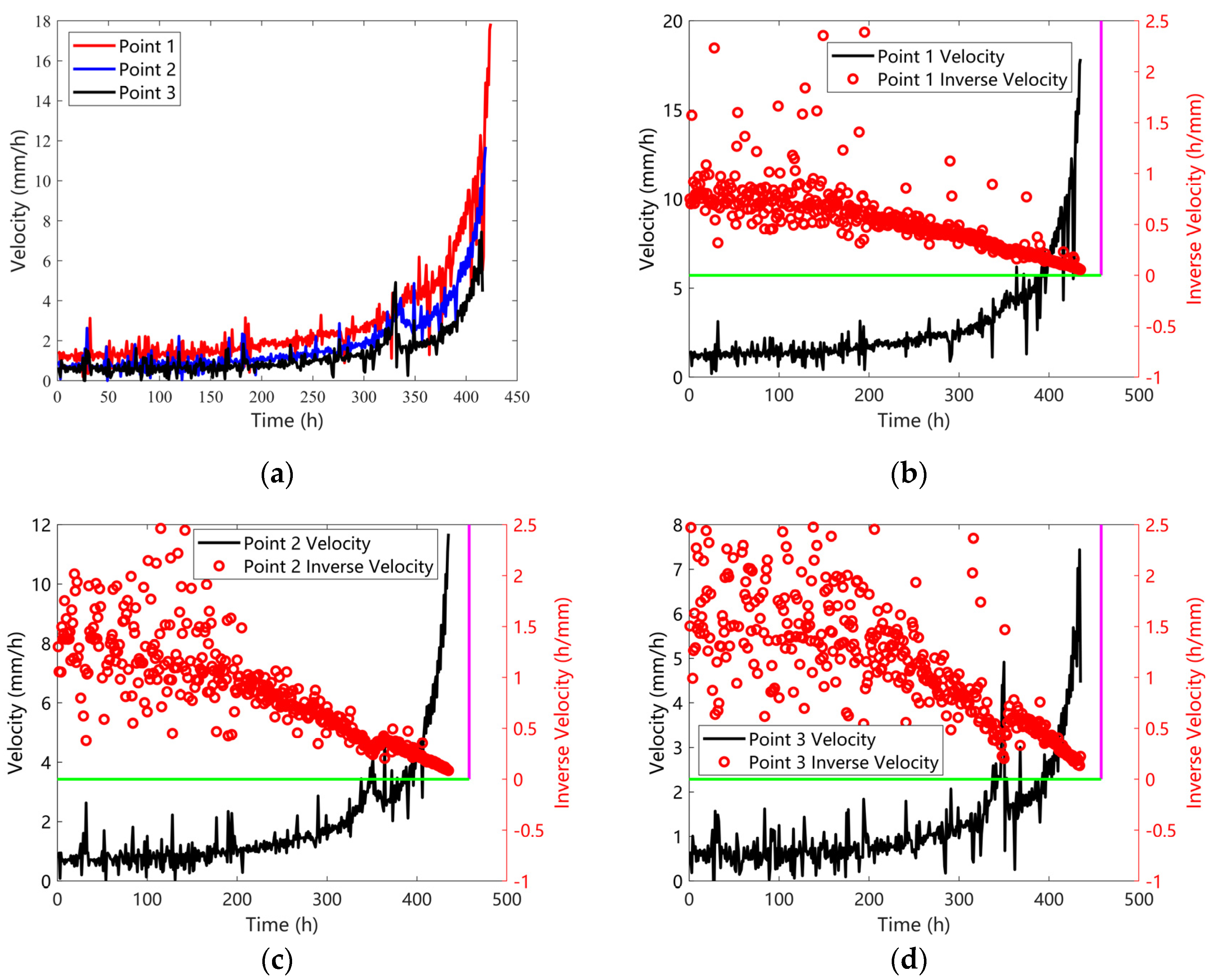
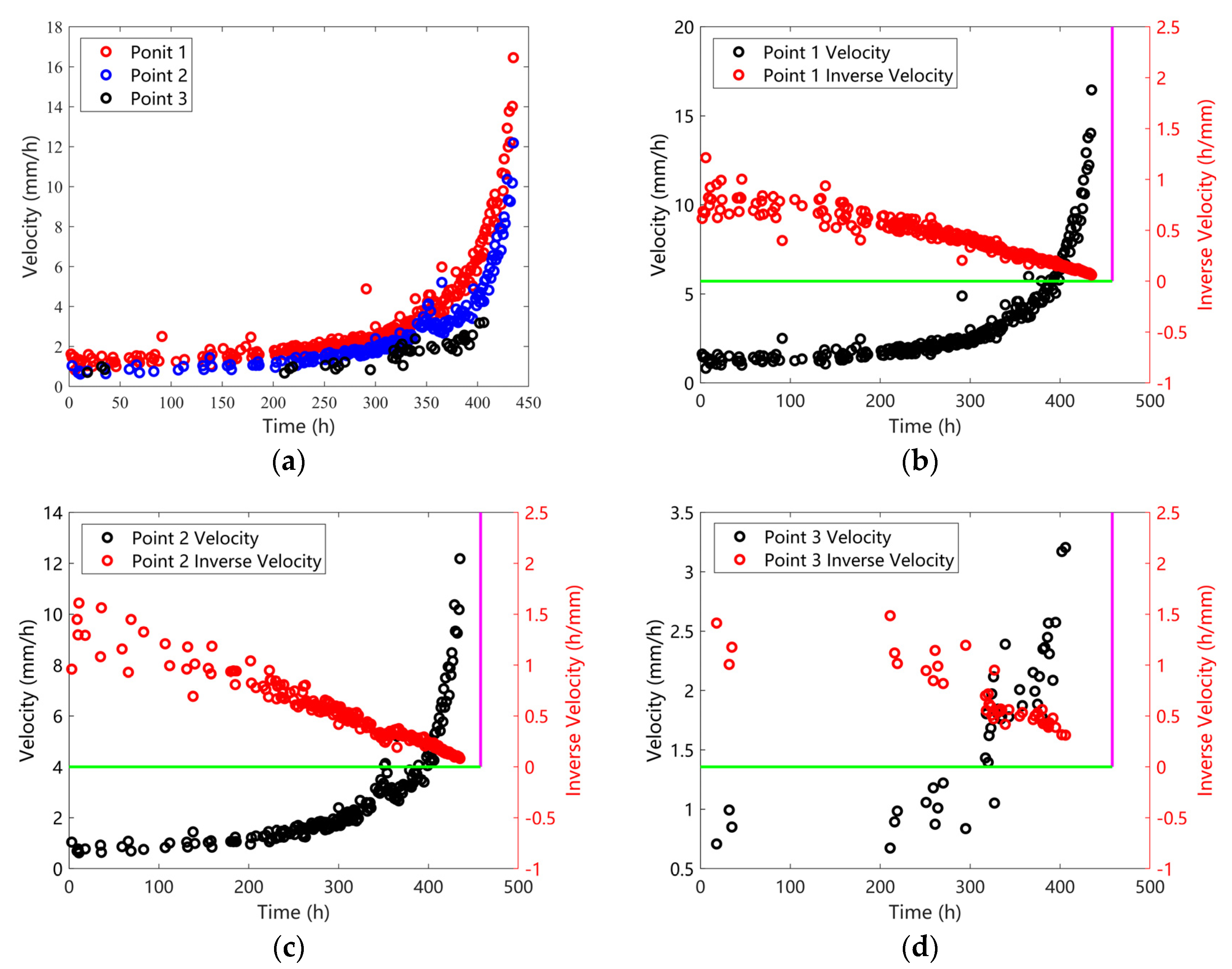
4.1. Single-Point Prediction Results

Three monitoring points were randomly selected within the landslide area to evaluate time-to-failure predictions using their velocities. Figure 6, Figure 7 and Figure 8 display the velocity distributions and inverse velocities for these points under three data-processing scenarios (Cases 1–3). As illustrated in Figure 6, Figure 7 and Figure 8, the velocity anomalies identified in Figure 4 persist across all cases, with inverse velocity plots exhibiting heightened sensitivity to these deviations. Distinct slopes of the inverse velocity fitting lines, such as those in Figure 6d and Figure 7d, reflect spatial heterogeneity in pre-failure deformation dynamics.

Table 2. Landslide prediction errors.

Prediction Errors (h)	Case 1	Case 2	Case 3
Point 1	1.98	−1.93	2.85
Point 2	−3.21	−3.97	−0.73
Point 3	−3.84	−1.92	−3.47

summarizes prediction errors (difference between predicted and actual failure times) for all three points across the data-processing scenarios.

As summarized in Table 1, prediction errors across the three monitoring points under all three operational scenarios predominantly range from −4 to +3 h. To evaluate the robustness and reliability of these outcomes, comparative error distributions were analyzed for forecasts generated at ten distinct temporal nodes during the final 10 h pre-failure phase (Figure 9).

Figure 9 illustrates the error distributions of failure time predictions across three monitoring points under Cases 1–3. Key observations include: (1) Prediction errors for all cases largely span −5 to +5 h, with Case 1 and Case 2 exhibiting pronounced variability at Point 1; and (2) Points 2 and 3 demonstrate relatively consistent errors (>2 h) across scenarios, though concurrent occurrences of premature (negative errors) and delayed (positive errors) predictions persist. This inconsistency, particularly the coexistence of over- and under-predictions, undermines definitive failure time determination, highlighting the necessity for developing more stable and reliable prediction methodologies.

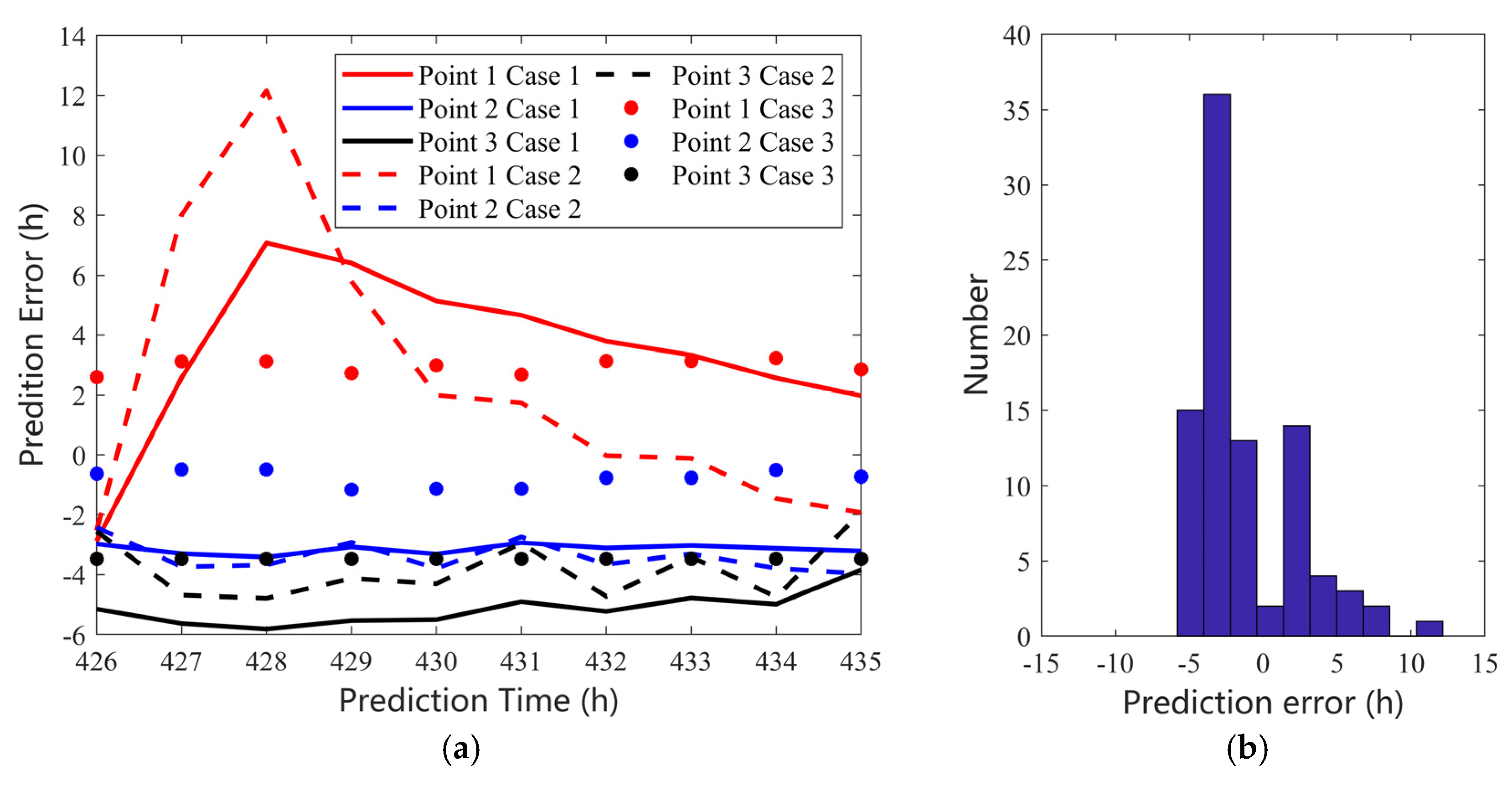
4.2. Multi-Point Joint Predictions

A nonlinear least squares algorithm was applied to integrate data from all 120 monitoring points. Predicted failure times under Case 1, Case 2, and Case 3 were 449.3 h (−8.7 h error), 450.7 h (−7.3 h error), and 458.3 h (+0.3 h error), respectively, demonstrating Case 3′s superior accuracy (Figure 10).

Figure 11 depicts the statistical distribution of the percentage of data exclusion at each monitoring point under Case 3. Despite data exclusion exceeding 50% at numerous monitoring points, the prediction accuracy remains uncompromised. Computations at this scale are not time-intensive, typically requiring only a few seconds.

Similar to single-point forecasting, the robustness and reliability of multi-point joint predictions necessitate rigorous validation. To this end, sensitivity analyses were conducted to evaluate: (1) Temporal Variability: The impact of prediction timing using temporal nodes consistent with Figure 10; and (2) Spatial Sampling Density: The influence of monitoring point inclusion ratios, tested at 10–90% increments (10% intervals).

For each density level (e.g., 90%), a non-repetitive 90% subset of monitoring points was randomly selected to generate ensemble predictions. This subsampling process was iterated 1000 times per density level to compute the mean prediction error and standard deviation across trials. The resultant error distributions, illustrating the interplay between spatial sampling density and temporal prediction stability, are presented in Figure 12.

As demonstrated in Figure 12, Case 1 exhibits mean prediction errors ranging from −8 h to +2 h, with standard deviations spanning 0–20 h, indicative of substantial uncertainty. Case 2 shows improved yet systematic prediction (mean error: −6 h to −3 h; standard deviation: 0–8 h). Notably, increasing the spatial sampling density in Cases 1 and 2 paradoxically amplifies mean errors while marginally reducing standard deviations. This counterintuitive behavior arises from the inherent limitations of rudimentary data exclusion and fitting strategies, where expanded datasets inadvertently propagate low-quality measurements, exacerbating prediction inaccuracies.

In stark contrast, Case 3 achieves exceptional stability, with mean errors confined to 0–2 h and standard deviations less than 3 h. Furthermore, prediction robustness improves with larger datasets: even at 10% sampling density, prediction errors remain within ±1 h, while higher data volumes further minimize standard deviations. These findings conclusively demonstrate that multi-point ensemble predicting delivers reliable and stable outcomes only when underpinned by rigorously selected data (Case 3), validating the necessity of advanced data-quality control protocols in operational landslide prediction systems.

5. Discussion

The accuracy of the INV is susceptible to multiple factors, including environmental noise in data acquisition and localized collapses near monitoring points [7]. The proposed multi-point group joint prediction method aims to mitigate the impact of such stochastic disturbances on single-point prediction accuracy by leveraging the enhanced robustness derived from integrated multi-point data analysis.

The multi-point group joint prediction method for landslide timing proposed in this study is not only applicable to scenarios where parameter α in the inverse velocity method equals 2 [13]. Theoretically, it can also be extended to cases where α is greater or smaller than 2 [6], though the selection and application should be determined based on the pre-failure velocity distribution patterns.

The temporal velocity datasets employed in this work may not represent the optimal choice. Alternative temporal resolutions, such as single-acquisition velocity, half-hourly velocity, or three-hourly velocity, could also be considered. However, excessively dense data may introduce significant noise interference, while overly sparse data may result in insufficient data points to ensure the stability of prediction outcomes.

This study utilized 120 spatial monitoring point groups within the landslide area. In practical engineering applications, S-SAR monitoring systems can cover millions of point groups [20], allowing for a substantially larger number of groups to be incorporated into the prediction framework. Following the methodology proposed here, real-time landslide monitoring systems could integrate data from thousands or even tens of thousands of point groups to generate highly robust time-of-failure predictions. Furthermore, for landslides monitored via alternative displacement measurement techniques, such as GNSS [23], multi-point displacement datasets could similarly be leveraged for joint prediction studies under the proposed framework.

6. Conclusions

This study systematically investigated landslide time prediction through both single-point and multi-point group joint predicting approaches, addressing three operational scenarios: simple data exclusion, velocity data fitting, and out-of-range data elimination. The principal findings are summarized as follows:

(1)

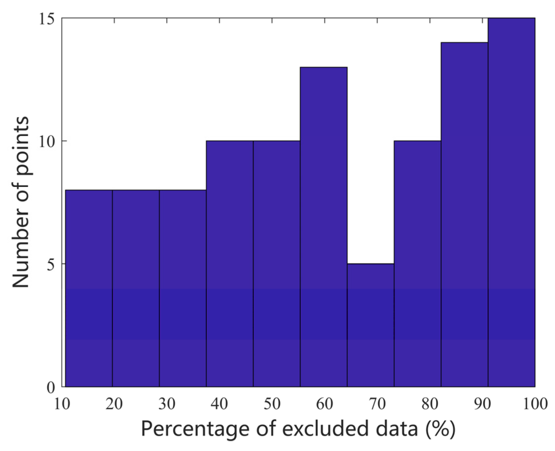
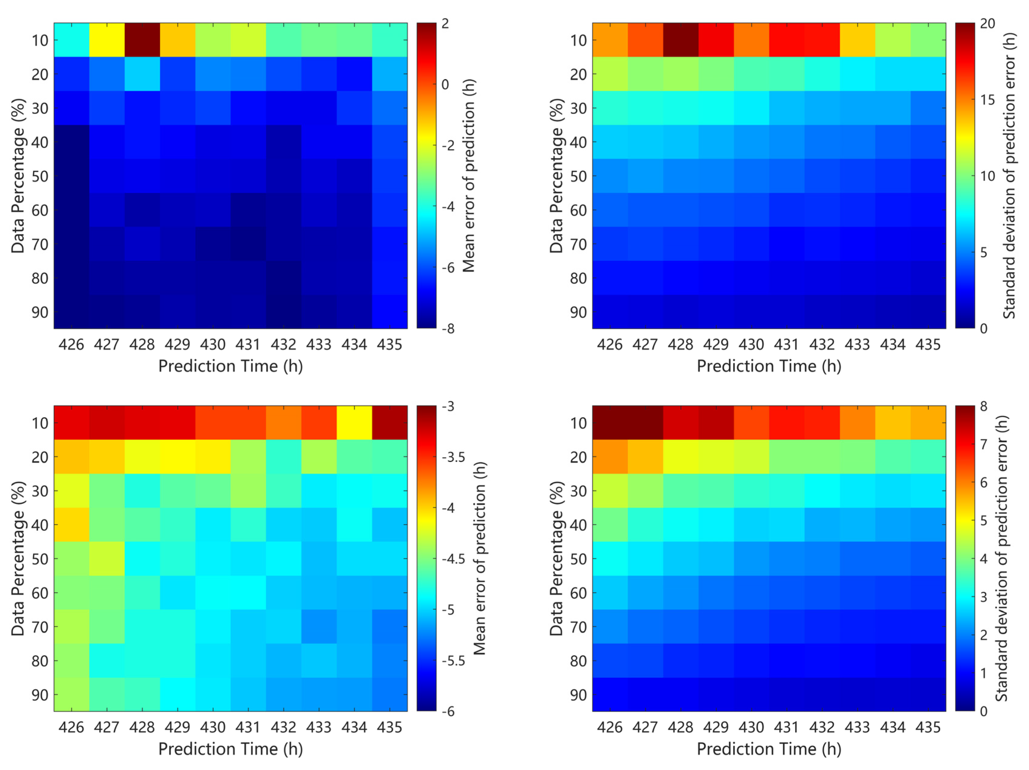
A novel multi-point joint inverse velocity method for landslide time prediction is developed, which achieves prediction errors consistently constrained within 1 h. Minimal discrepancies (<2 h) were observed based on strict data exclusion, with enhanced stability and reliability emerging proportionally to the number of displacement monitoring points incorporated.

(2)

Point groups distributed across different landslide sectors can all be utilized for inverse velocity method-based failure time prediction, with variations in the slope of the inverse velocity fitting line reflecting spatial heterogeneity.

(3)

Single-point deformation velocity monitoring data yield inverse velocity method predictions with stochastic error distributions and limited stability.

References

1. Gong, W.; Zhang, S.; Juang, C.H.; Tang, H.; Pudasaini, S.P. Displacement prediction of landslides at slope-scale: Review of physics-based and data-driven approaches. Earth-Sci. Rev. 2024, 258, 104948. [Google Scholar] [CrossRef]
2. Fukuzono, T. A simple method for predicting the failure time of slope using reciprocal of velocity. Technol. Disaster Prev. Sci. Technol. Agency 1989, 13, 111–128. [Google Scholar]
3. Zhou, X.P.; Liu, L.J.; Xu, C. A modified inverse-velocity method for predicting the failure time of landslides. Eng. Geol. 2020, 268, 105521. [Google Scholar] [CrossRef]
4. Wang, J.-Z.; Ju, N.-P.; Tie, Y.-B.; Bai, Y.-J.; Ge, H. A framework for identifying the onset of landslide acceleration based on the exponential moving average (EMA). J. Mt. Sci. 2023, 20, 1639–1649. [Google Scholar] [CrossRef]
5. Tao, Y.; Zhang, R.; Du, H. Failure Prediction of Open-Pit Mine Landslides Containing Complex Geological Structures Using the Inverse Velocity Method. Water 2024, 16, 430. [Google Scholar] [CrossRef]
6. Petley, D.N.; Bulmer, M.H.; Murphy, W. Patterns of movement in rotational and translational landslides. Geology 2002, 30, 719–722. [Google Scholar] [CrossRef]
7. Rose, N.D.; Hungr, O. Forecasting potential rock slope failure in open pit mines using the inverse-velocity method. Int. J. Rock Mech. Min. Sci. 2007, 44, 308–320. [Google Scholar] [CrossRef]
8. Dick, G.J.; Eberhardt, E.; Cabrejo-Liévano, A.G.; Stead, D.; Rose, N.D. Development of an early-warning time-of-failure analysis methodology for open-pit mine slopes utilizing ground-based slope stability radar monitoring data. Can. Geotech. J. 2015, 52, 515–529. [Google Scholar] [CrossRef]
9. Wang, Y.P.; Xu, Q.; Zheng, G.; Zheng, H. A rheology experimental investigation on early warning model for landslide based on inverse-velocity method. Rock Soil Mech. 2015, 36, 1606–1614. [Google Scholar]
10. Iwat, N.; Sasahara, K.; Watanabe, S. Improvement of Fukuzono’s Model for Time Prediction of an Onset of a Rainfall-Induced Landslide. In Proceedings of the 4th World Landslide Forum, Ljubljana, Slovenia, 30 May–2 June 2017. [Google Scholar]
11. Qi, L.; Tan, W.; Huang, P.; Xu, W.; Qi, Y.; Zhang, M. Landslide prediction method based on a ground-based micro-deformation monitoring radar. Remote Sens. 2020, 12, 1230. [Google Scholar] [CrossRef]
12. Zhang, J.; Wang, Z.; Hu, J.; Xiao, S.; Shang, W. Bayesian machine learning-based method for prediction of slope failure time. J. Rock Mech. Geotech. Eng. 2022, 14, 1188–1199. [Google Scholar] [CrossRef]
13. Ma, H.T.; Zhang, Y.H.; Yu, Z.X. Research on the identification of acceleration starting point in inverse velocity method and the prediction of sliding time. Chin. J. Rock Mech. Eng. 2021, 40, 355–364. [Google Scholar]
14. Du, H.; Song, D. Investigation of failure prediction of open-pit coal mine landslides containing complex geological structures using the inverse velocity method. Nat. Hazards 2022, 111, 2819–2854. [Google Scholar] [CrossRef]
15. Sharifi, S.; Macciotta, R.; Hendry, M.T. Critical assessment of landslide failure forecasting methods with case histories: A comparative study of INV, MINV, SLO, and VOA. Landslides 2024, 21, 1629–1643. [Google Scholar] [CrossRef]
16. Voight, B. A method for prediction of volcanic eruptions. Nature 1988, 332, 125–130. [Google Scholar] [CrossRef]
17. Voight, B. A relation to describe rate-dependent material failure. Science 1989, 243, 200–203. [Google Scholar] [CrossRef]
18. Massonnet, D.; Feigl, K.L. Radar interferometry and its application to changes in the Earth’s surface. Rev. Geophys. 1998, 36, 441–500. [Google Scholar] [CrossRef]
19. Osasan, K.S.; Afeni, T.B. Review of surface mine slope monitoring techniques. J. Min. Sci. 2010, 46, 177–186. [Google Scholar] [CrossRef]
20. Severin, J.; Eberhardt, E.; Leoni, L.; Fortin, S. Development and application of a pseudo-3D pit Slope displacement map derived from ground-based Radar. Eng. Geol. 2014, 181, 202–211. [Google Scholar] [CrossRef]
21. Caduff, R.; Schlunegger, F.; Kos, A.; Wiesmann, A. A review of terrestrial radar interferometry for measuring surface change in the geosciences. Earth Surf. Process. Landf. 2015, 40, 208–228. [Google Scholar] [CrossRef]
22. Carlà, T.; Intrieri, E.; Di Traglia, F.; Nolesini, T.; Gigli, G.; Casagli, N. Guidelines on the use of inverse velocity method as a tool for setting alarm thresholds and forecasting landslides and structure collapses. Landslides 2017, 14, 517–534. [Google Scholar] [CrossRef]
23. Gül, Y.; Hastaoğlu, K.Ö.; Poyraz, F. Using the GNSS method assisted with UAV photogrammetry to monitor and determine deformations of a dump site of three open-pit marble mines in Eliktekke region, Amasya province, Turkey. Environ. Earth Sci. 2020, 79, 248. [Google Scholar] [CrossRef]
Figure 1. Schematic diagram of Inverse Velocity Method.
Applsci 15 07449 g001
Figure 2. Image of the slope radar.
Applsci 15 07449 g002
Figure 3. (a) Slope displacement monitoring cloud map, the area surrounded by blue lines is the landslide area, and the blue dots are the three points used for single point prediction study (b) Photo of landslide.
Applsci 15 07449 g003
Figure 4. Randomly selected point group displacement curve and velocity curve. Different colored lines represent different monitoring points. The red rectangle in (b) represents the interval of velocity anomalies.
Applsci 15 07449 g004
Figure 5. Schematic diagram of velocity processing under different cases. Different colored lines/circles represent different monitoring points.
Applsci 15 07449 g005
Figure 6. (a) Velocity curves of different points (b) Velocity and inverse velocity of point 1 (c) Velocity and inverse velocity of point 2 (d) Velocity and inverse velocity of point 3. The pink line represents the time when the landslide occurred. The green line represents the position where the inverse velocity is 0.
Applsci 15 07449 g006
Figure 7. (a) Velocity curves of different points (b) Velocity and inverse velocity of point 1 (c) Velocity and inverse velocity of point 2 (d) Velocity and inverse velocity of point 3. The pink line represents the time when the landslide occurred. The green line represents the position where the inverse velocity is 0.
Applsci 15 07449 g007
Figure 8. (a) Velocity distribution of different points (b) Velocity and inverse velocity of point 1 (c) Velocity and inverse velocity of point 2 (d) Velocity and inverse velocity of point 3. The pink line represents the time when the landslide occurred. The green line represents the position where the inverse velocity is 0.
Applsci 15 07449 g008
Figure 9. (a) Error distribution of landslide prediction time at 10 different moments for 3 spatial points under 3 cases. (b) The statistical chart of (a).
Applsci 15 07449 g009
Figure 10. Schematic diagram of multi-point joint prediction results under 3 cases. The dots of different colors represent the inverse velocity data of different monitoring points, and the corresponding color lines are the fitted lines of these dots.
Applsci 15 07449 g010
Figure 11. Statistical distribution of the percentage of data exclusion at each monitoring point under Case 3.
Applsci 15 07449 g011
Figure 12. Stability test results of multi-point joint prediction.
Applsci 15 07449 g012aApplsci 15 07449 g012b