1. Introduction
A Digital Twin (DT) has been defined as “the creation of virtual models for physical objects in a digital way to simulate their behaviors” [
1]. Essentially, a DT is a digital replica that models reality, thus providing a clear picture of the physical system being analyzed, recording its history, and serving as a powerful platform for decision-making and experimentation. Digital twins can be used for a wide range of applications such as manufacturing, aviation, healthcare, communication networks, Intelligent Transportation Systems (ITS), and urban intelligence, among others, and are characterized by three components: the physical world or object, its digital (virtual) counterpart, and the communication channel between them (cf.
Figure 1). A bidirectional communication between both physical and digital worlds is a key aspect of a digital twin, as the physical world must feed information to the virtual world so that it is able to update its state in real-time, to perform tests or training, and to send the results back to the physical world.
This paper presents the development, analysis, and validation of a transportation digital twin, where transportation modelling or transportation digital twin is one of the functions of ITS. A transportation digital twin keeps a digital copy of a road, highway, village, or city in real-time and has numerous applications. Notably, these include digital twins used for simulating autonomous vehicles in real-world conditions [
2], monitoring and predicting future traffic situations [
3], road planning [
4], and optimizing traffic and road safety [
5]. However, it is important to note that the majority of the digital twin applications are used to address microscopic aspects, which involve the application between individual vehicles. There is relatively little research on macroscopic traffic control, which involves managing large-scale transportation systems, including overall traffic flow and congestion patterns [
6]. A more detailed review and classification of transportation digital twins is provided in
Section 2, focused on the state of the art.
A transportation digital twin requires real-time data to accurately reflect real-world conditions. This data is provided by sensors located along the road or through Vehicle-to-Everything (V2X) communications from connected vehicles. Connected vehicles send periodic Cooperative Awareness Messages (CAMs) to inform precisely of their position, whereas information from sensors can provide the number of vehicles passing through a specific point of the highway. Whether using V2X communications, sensors, or both, the digital twin uses this information to make decisions. These decisions are then transmitted back to the physical system using Vehicle-to-Infrastructure (V2I) communication via Infrastructure to Vehicle Information Messages (IVIM), and are also communicated to drivers through a mobile application developed by the road operator, which uses the cellular communication network. This dual-channel communication closes the loop between the physical and virtual worlds, enabling real-time feedback and action.
To the best of our knowledge, there is no other study in the literature that develops a complete interurban digital twin that uses real highway data to make decisions to improve traffic congestion efficiency and minimize environmental impact in a macroscopic manner. Motivated by this context, in this work, we develop a transportation digital twin that replicates a segment of the C-32 highway in Barcelona (Spain), with the objective of mitigating traffic congestion and reducing pollution emissions by applying specific traffic strategies such as changing the speed limit and recommending vehicle re-routing on the highway. Specifically, the work presented in this paper is focused on the following:
- -
Development of a transportation digital twin to reduce traffic congestion and pollution emissions.
- -
Proposal and validation of traffic strategies applied by the digital twin for improving performance.
- -
Definition and evaluation of Key Performance Indicators (KPI) for selecting the best traffic strategy.
- -
Design and validation of the decision-making algorithm for strategy selection.
- -
Validation of the digital twin implementation
The remainder of this paper is organized as follows. The state of the art of transportation digital twins is summarized in
Section 2, where the main approaches of developed transportation digital twins are presented. Then, the proposed architecture is introduced in
Section 3. Once the general idea is presented, the development of the digital twin is described in
Section 4. The evaluation scenario is exposed in
Section 5. The performance evaluation, including the algorithm for deciding the strategy to apply, is presented in
Section 6. Finally,
Section 7 contains the validation of the digital twin implementation in real-time. To conclude the paper, the conclusions and future work are presented in
Section 8.
2. State of the Art on Digital Twins for Intelligent Transportation Systems
This section presents the state of the art of transportation digital twins. Before characterizing the latest studies in this area, it is important to know where the concept of digital twins comes from. The first public mention of the concept of digital twin was made in 2002 by M. Grieves at the Society of Manufacturing Engineers conference in Michigan [
7]. The digital twin that M. Grieves proposed was a model to manage the product lifecycle. Although already defined, the term digital twin was established by J. Vickers of NASA in 2010, where it was used to improve the physical model of the spacecrafts [
8]. Since then, digital twins have been developed in many different areas, such as industry 4.0 [
9], agriculture [
10], healthcare [
11], ITS [
6], and urban intelligence [
4], among others. In ITS, several studies, depicted in the following subsections, have been carried out involving transportation digital twins. Some of them are merely a proof of concept, while others have been implemented in small environments to test their capabilities and limitations. Nowadays, we even have real implementations of digital twins of cities, which are mainly used for urban planning purposes. Transportation digital twins can be classified into four categories: urban scenarios, interurban scenarios, autonomous vehicles, and other prototypes.
2.1. Digital Twins of Urban Scenarios
Urban case studies focus on the development of a digital twin of a city or a specific section of it. In this field, several research works have been conducted. For instance, ref. [
12] develops a digital twin for Adaptive Traffic Signal Control (ATSC). This digital twin contains the traffic signal controller, the roads, and the updated information of the vehicles and their trajectories. The digital twin processes the information and decides how to change the traffic lights, which is communicated to the traffic controller in the real world. The metric optimized by this digital twin is the Average Accumulated Waiting Time (AAWT), defined as the total waiting time that the vehicle has experienced at all its stops. The platform used for simulation is Simulation of Urban Mobility (SUMO) [
13]. This work only presents a theoretical case study; no demonstration has been carried out to prove its viability.
The work in [
14] presents another urban study that focuses on non-signalized intersections. This work designs a cooperative driving system for non-signalized intersections with the objective of avoiding full stops for connected vehicles. Two main modules are proposed: a motion module in charge of map matching with Unity [
15], path planning, and scheduling of the sequence of vehicles to cross the intersection using enhanced First In First Out (FIFO) slot reservation; and a communication module, which analyses performance and tracks communication issues. The V2X connectivity is based on Dedicated Short-Range Communications (DSRC), Cellular V2X (C-V2X), or both. In addition, augmented reality for Human–Machine-Interface (HMI) is designed to provide guidance to the drivers. Two case studies are performed, one using a map of San Francisco, and the other involving Human-In-The-Loop (HITL) simulation.
The work in [
16] proposes a digital twin methodology to perform multi-vehicle experiments, which involves the coordinated control of several vehicles and addresses the limitations of field testing in cooperative vehicle control. A cloud platform is used to collect real-world data, and time delay and mapping accuracy are evaluated. The HMI uses web services and augmented reality (HoloLens) to visualize the digital twin. To support the HMI, the game engine Unity3D 6.1 (6000.0.47f1) is used to provide a more immersive experience. To test this method, a prototype consisting of a sand table testbed is developed, along with its corresponding twin system and a driving simulator.
The work in [
17] creates an Urban Digital Twin (UDT) to closely resemble the real world. It is a proposal for the data acquisition and representation phase, but no further processing is done with the information. The main objective is to reproduce in 3D the desired time and place by adding individual pedestrians and vehicles to the UDT model. Monocular camera lens-based Closed-Circuit Television (CCTV) is used to collect the data of the individual objects, and Unity3D is used for visualization.
Real implementations of urban digital twins are currently under development, with European initiatives such as Digital Urban European Twins (DUET) [
18], which aims to build digital twins of three cities (Flanders, Pilsen, and Athens) to understand the relationship between traffic, air quality, noise, and other urban factors. Similarly, the Low-Emission Adaptive last mile logistics supporting the ‘on Demand economy’ through digital twins (LEAD) project [
19], is developing digital twins for six cities (Madrid, The Hague, Budapest, Lyon, Oslo, and Porto), with the objective of providing smart urban logistics that are more environmentally, socially, and economically sustainable. Several Russian cities are using the RITM3 platform to develop their own digital twins, and other cities such as Amaravati and Singapore are also in the process of creating their own.
2.2. Digital Twins of Interurban Scenarios
Interurban case studies include highways or tunnels. The work in [
20] proposes a digital twin of a road section to facilitate vehicles to cooperate with each other before arriving at a merging zone. The cloud contains a pre-built map of the road section, and the vehicle’s coordinates are uploaded and matched to the map. Vehicle-to-cloud communication is facilitated by the 4G/LTE cellular network. The work proposes algorithms to calculate the optimal merging, in which neither of the vehicles involved must perform abrupt accelerations/decelerations (only longitudinal planning, so lane changes are not considered), but no intelligence or simulation is involved. The final decision is sent to the driver’s HMI display, which shows the recommended speed. A field implementation was conducted in Riverside, California, with three passenger vehicles, two on the main lane and one on the ramp.
The work in [
21] aims to construct a digital twin of a tunnel with the purpose of analyzing traffic flow, preventing traffic jams inside the tunnel, and taking care of accidents and facility management. Building Information Modelling (BIM) technology was used to construct the model of the tunnel, and a 3D real-time fusion method is proposed, which involves obtaining data from video acquisition, the tunnel geometry model, and point calibration information. Decisions made in the cloud are sent in real time to drivers to recommend safer and more efficient driving. A field implementation was carried out in China with three passenger vehicles.
2.3. Digital Twins in Autonomous Vehicles
Another important application of digital twins is to speed up the development and testing of autonomous vehicles. The work presented in [
22] identifies a gap between virtual environments and self-driving platforms and proposes a solution by introducing a Hardware-in-the-Loop (HiL) simulation system. To achieve this, the same Electronic Control Units (ECUs) found in self-driving vehicles are used in the closed loop of offline simulation. As a result, the offline simulation performs very similarly to the actual autonomous vehicle, and algorithms are implemented more quickly into self-driving vehicles. The study uses decision-making and path planning algorithms without machine learning.
2.4. Other Prototypes
Other studies that do not fall into either of the previous categories have also been designed. In [
23], a prototype for a real-time digital twin of the traffic environment is presented. The implemented system provides, as the main service, the visualization of the digital twin with a 3D simulation, so the focus is on data acquisition and digital twin building. There is no decision-making or simulation. The methodology used is based on a proposed architecture, which includes a cloud server and wireless sensors connected to it, called the Central Perception System Architecture. This communication is over 5G or DSRC using SENSORIS [
24] message format. Unity is used for visualization. A simple field implementation has been carried out with a central server in the cloud and three sensors.
Similarly, the work in [
25] identifies the steps needed to generate a highly accurate digital twin. Three different test fields are implemented: urban, rural, and highway. Data is acquired and forwarded in real time through 4G and ITS-G5 to a central computing server to update the digital twin. Data management is performed with the open-source Apache NiFi project. Only the data acquisition and updating of the digital twin are presented.
In [
26], the authors propose a framework for a Mobility Digital Twin (MDT). The physical space contains sensors, cameras, and LiDARs, and their samples are sent to the digital space. The digital space is in charge of storage, modelling, learning, simulation, and prediction. Machine learning is applied to learn performance and preference for vehicles. A cloud-edge architecture is used to enable faster updates. An example of a cloud–edge architecture is implemented with Amazon Web Services (AWS), and a case study on personalized adaptive cruise control is performed.
Finally, the work in [
27] tries to solve two problems in implementing digital twins. The first is that in a real transportation environment, vehicles have different levels of automation (vehicular heterogeneity), and the second is that a digital twin requires large quantities of computation, which implies high delay. To tackle both problems, a digital twin-empowered edge AI framework is proposed. This framework consists of three domains: vehicle, edge AI, and digital twin domains. Real-time responsiveness is guaranteed in the edge AI domain. The digital twin domain performs more advanced algorithms, such as deep reinforcement learning, to improve traffic efficiency. SUMO, with OMNeT++, is used for simulating the decisions made by intelligent algorithms. The paper does not present a field implementation.
To conclude, there are many studies in the literature in the area of transportation digital twins. Some of these studies focus on creating a digital replica to monitor and understand the real world but do not complete the loop from the digital world back to the real world, while others emphasize decision-making processes that are injected back into the real world. Notwithstanding, these studies bring us a step closer towards understanding the feasibility and intricacy of building a real-time digital twin that incorporates decision-making software. However, it can be noticed that most of the research has concentrated on the study of microscopic use cases, which are addressed to individual vehicles. Nonetheless, there exists a research gap in the exploration of macroscopic-level control decisions aimed at coordinating and optimizing highway systems, which our study tries to address.
3. Digital Twin Architecture Proposal for Interurban Intelligent Transportation Systems
The objective of building the digital twin proposed in this paper is to mitigate incidents on the highway by making recommendations to the drivers. The digital twin follows the basic framework for DTs, consisting of a real world containing cameras, sensors, and other devices to detect vehicles, and a digital world that replicates the real world. This digital world receives input data from connected vehicles and from the roadside infrastructure on the highway. The data is processed and used to predict whether there is a congestion or pollution incident on the highway. When an incident is detected, a trigger is set off, which will turn on simulation work, including real-time vehicle data on the highway and the detected incident. According to the output of this simulation analysis, a strategy will be recommended to mitigate the effect created by this incident.
Figure 2 shows the proposed digital twin architecture. The Aggregation module, as its name suggests, receives and aggregates data from different sources. The Pre-Processing module pre-processes the data and transforms it into the needed format. From the traffic patterns, this module can also detect the incident, or a manual input for the incident detection can be employed. When an incident is detected, a trigger is sent to the Traffic Simulator module to activate it. Aimsun Next [
28] has been chosen as the simulation tool. The simulator receives the pre-processed data and the incident, and runs simulations to test the different strategies. The outputs of these simulations are sent to the Decision Engine, which will decide the best strategy to reduce congestion or pollution levels, based on the cause of the incident. This strategy is sent to the real world through informative panels on the highway or to connected vehicles.
We have considered two use cases to address the two types of incidents assessed by our digital twin: the congestion use case and the pollution use case.
3.1. Congestion Use Case
In the congestion use case, the study focuses on a traffic scenario where there is an incident that creates congestion on the highway. For this use case, the input data has been provided by the road operator of the highway. It has the necessary infrastructure to obtain information about the number of vehicles on the highway through cameras and sensors in its entrances and exits.
Possible strategies to reduce congestion consist of giving speed recommendations, re-routing vehicles off the highway, or opening additional lanes on the highway. Reducing speed limits in a particular situation, also referred to as Variable Speed Limits (VSL), is a common technique used to reduce congestion [
29]. Reducing speed limits when there is a heavy traffic situation increases road capacity. Moreover, slower speed limits result in more comfortable driving, so vehicles are closer together, increasing road capacity and minimizing stop-and-go situations. Consequently, travel times are reduced because there is less congestion. In addition, on congested highways, variable speed limits have proven to be safer and reduce accidents. Tests performed in Germany [
30] show that travel times are reduced by 5–15% and collisions by 30% when this technique is applied.
On the other hand, in incident situations, where one or more lanes have been blocked, the capacity of the highway is reduced, so the only option to reduce congestion is for some vehicles to exit the highway. Alternative routes may be offered to decrease the number of vehicles on the highway.
Another viable solution is to increase road capacity by opening additional lanes. This can be done by either converting the road’s shoulder into an additional lane or using a lane from the opposite direction of the highway. However, there are some limitations when executing this strategy in real time. Opening additional lanes must be a premeditated decision, done when congestion is expected, for example, during the holiday season when many vehicles leave the city. In such cases, the road has to be prepared and signalized, and safety must be ensured, so it cannot be implemented in real time according to spontaneous congestions or incidents on the highway.
As a result, the traffic strategies that we have applied in this work consist of the following: (1) speed recommendations; and (2) re-routing of vehicles. Lower speed recommendations can be applied to the section of the highway where the incident is located, or to a larger part of the highway by also limiting previous sections. Both speed recommendation strategies have been implemented. In addition, when re-routing vehicles, this strategy is considered as a percentage of vehicles exiting the highway.
3.2. Pollution Use Case
The purpose of this second use case is to utilize the digital twin to recommend strategies to drivers that can help mitigate pollution episodes.
Aimsun Next [
28] includes the emission model COPERT [
31], providing estimations of emissions caused by vehicles in each simulation. The pollutants available are carbon monoxide (CO), nitrogen oxides (NO
x), and particulate matter (PM), specifically particles with a maximum diameter of 2.5 μm (PM
2.5).
For this use case, the strategy used to achieve a reduction in emission levels is variable speed limits. Maintaining a moderate speed and a constant pace helps reduce pollution, as vehicles consume less fuel when traveling at steady speeds. Speeds between 70 and 90 km/h are generally considered the most effective for minimizing emissions and maximizing fuel efficiency. However, this optimal speed range can vary depending on factors such as vehicle type, engine design, and driving conditions. Additionally, the most convenient speed limit for mitigating emissions may change in response to real-time traffic conditions. In this way, a study conducted in Barcelona [
32] indicates that the reduction of the speed limit to 80 km/h, implemented in 2008 in certain areas, caused an increase in NO
x and PM
10 levels, while variable speed policies helped reduce these emission levels. This is why variable speed limits play a crucial role, offering a more responsive, adaptive, and efficient approach to managing traffic-related pollution by adjusting to current conditions and ensuring vehicles operate within their most efficient speed range.
Speed limits, as in the first use case, are modified not only on the incident section, but also on some of the previous sections of the highway.
4. Digital Twin Implementation
In the following, we present the implementation details of the two main elements of the DT, with
Section 4.1 focusing on the Traffic Simulator module, and
Section 4.2 on the Decision Engine module. For the evaluation and development of these modules, we consider a manual input of the incidents detected by the Pre-processing module, together with the use of historical data for the traffic information needed. Upon completion, the developed modules will operate with real-time data sourced from the sensors of the highway and will be triggered by the detection of different kinds of incidents.
4.1. Traffic Simulator Module
To feed the digital twin presented in this paper, traffic data from sensors deployed along the C-32 highway has been used. The data includes vehicle intensity (vehicles per hour) at each entrance, exit, and turn of the highway, with a 5-min resolution. These data enter the Traffic Simulator through the Pre-processing module shown in
Figure 2.
The Aimsun Next tool [
28] is used to simulate highway traffic and to test different strategies. Aimsun Next is a powerful multi-resolution and multi-modal mobility simulator capable of simulating any personalized scenario. The highway has been recreated in the simulator by building a map divided into different sections, each located between two consecutive entrances and exits of the highway (cf.
Section 5). The map has been created by specifying the location, length, shape, and speed limit of each section. The traffic data measured in these sections has been processed to apply the strategies to improve different parameters depending on the type of incident, i.e., congestion or pollution.
To study the impact of incidents over a long period of time and to test possible ways to alleviate their effects, we have chosen to conduct simulations that replicate the real traffic conditions for 1 h. The input data, collected at 5-min intervals, consists of traffic flows of vehicles entering, exiting, and turning at highway entrances and exits. The simulations start with an empty map and have an additional transitory period until the vehicles fill the road and reach a permanent regimen. Each simulation is performed 10 times, changing the initial seed, and averaging the results.
Different vehicle types can be inserted into the simulation. The pollution use case considers trucks, cars, and motorbikes. In addition, other characteristics related to the vehicles can also be specified, such as speed limit, acceptance of the speed limit, and cooperation with other vehicles. Vehicle type percentages must also be defined to provide more realistic results, especially when calculating vehicle emissions.
Incidents are detected in the Pre-processing module and are replicated in the simulator to reproduce the real scenario. They can be placed at any point on the map to simulate an accident, with specific configurations for location, duration, length, and lane of the incident.
The simulator module outputs the following KPIs for performance evaluation: vehicle travel time, defined as the duration a vehicle requires to complete its journey; vehicle speed; vehicle speed deviation, defined as the difference in speeds between vehicles traveling in the same direction; number of vehicles in the highway; vehicle intensity, measured as the number of vehicles per hour; vehicle occupancy, defined as the number of vehicles per km; and emission levels for the pollutants CO, NOx, and PM2.5, expressed as g/km. The KPIs are collected and averaged across the entire highway in the direction of the incident and are defined as total travel time, average speed, average speed deviation, average number of vehicles, average intensity, average occupancy, average CO, average NOx, and average PM2.5.
4.2. Decision Engine Module
To select the optimal traffic strategy, the above KPIs are evaluated across the different available traffic strategies.
For the congestion use case, the optimal strategy is the one that provides maximum average speed and minimum average speed deviation between cars circulating on the highway. Low values for average speed deviation ensure that all vehicles drive at similar speeds, which will make the highway more secure. For this purpose, an additional KPI called Speed-Dev-Ratio, consisting of the relationship between the average speed of vehicles and their deviation, has been considered as follows:
Optimal performance corresponds to higher speeds and less deviation, so a higher value of Speed-Dev-Ratio is expected. Higher average intensity is better, as more vehicles per hour means higher speeds. Differently, the lower the average occupancy, the better, as it means that speed can be higher. As occupancy and intensity are proportional, only intensity is considered to make the decision. The number of vehicles is directly related to the intensity, so the former is not considered. The final KPI considered is the total travel time. As expected, the optimal total travel time corresponds to the minimum value.
On the other hand, for the pollution use case, different KPIs are monitored during the decision-making process. In this case, the most effective traffic strategy is the one that achieves the greatest reduction in the levels of the three pollutants (CO, NOx, and PM2.5). Although the objective of this use case is to mitigate emissions, traffic parameters are monitored as well to avoid significant traffic disruptions. For that reason, the total travel time KPI is also considered when selecting the best traffic strategy to minimize emissions.
5. Evaluation Scenario
This section defines the evaluation scenario.
Section 5.1 describes the study area, input data, and incident modeling.
Section 5.2 presents the simulation setup for the congestion use case, and
Section 5.3 outlines the simulation design for the pollution use case.
5.1. Study Area and Data
The proposed digital twin was evaluated on a 13 km segment of the C-32 highway in Spain, considering different traffic scenarios. The input data was provided by the highway’s traffic operator through a dataset from January to December 2022.
Figure 3 illustrates the traffic data at a specific point on the highway, showing the number of vehicles detected at the main toll in each direction. The top plot represents northbound traffic, while the bottom plot shows southbound traffic. Weekdays are shown in blue and weekends in gray. This visual distinction highlights typical weekly patterns as well as seasonal variations, particularly the increase in southbound volume during summer months.
A key limitation in this study is the absence of recorded data corresponding to real-world incidents involving extreme congestion, as the highway operator does not maintain such records. This lack of empirical data restricts the ability to analyze system behavior under high-demand conditions. To overcome this limitation, we apply scaling factors to the available traffic data. This approach maintains the original temporal and spatial characteristics of observed traffic patterns while systematically increasing traffic intensity. In doing so, it provides a controlled means of simulating congested scenarios without resorting to entirely synthetic flows or hypothetical demand profiles.
The 13 km of the highway are divided into sections, represented in
Figure 4 with red lines. These sections are defined between entry and exit points, where sensors are placed to detect vehicles entering and exiting the highway. Additionally, to be able to test scenarios where the congestion has been caused by incidents, a specific type of incident has been defined and placed at various locations along the highway. This incident represents a scenario where the highway has two lanes available, but one lane is fully blocked for the entire simulation duration, either due to an accident, roadwork, or a disabled vehicle. Driver behavior in response to the incident is modeled using the two corner cases defined in this study: full compliance (where all vehicles follow the recommended strategy) and full non-compliance (baseline, where no vehicle responds).
Figure 4 shows the locations of the tested incident A.
5.2. Simulation Design for Congestion Use Case
We performed two sets of simulations for the congestion use case. The aim of the first set is to analyze the performance of three scenarios (each scenario with a different scaling factor) across different traffic strategies, while the second set is a batch of scenarios to design the decision-making algorithm.
The results of the first set of simulations, discussed in
Section 6.1, were obtained in two different scenarios: (i) without any traffic congestion or incidents; and (ii) with incident A located at the end of section S_6, as shown in
Figure 4. The input data used for these simulations corresponds to the most congested hour and day in the 2022 dataset for the southbound direction, which was on 23 June 2022, at 17 h (cf.
Figure 3). Scaling factors of 5, 4.75, and 4.5 were applied to this data. For each scenario, we tested different traffic strategies. The objective is to analyze and familiarize the behavior of the KPIs to decide the best strategy to mitigate congestion. The tested traffic strategies are as follows: (a) reducing the speed limit (from 120 km/h down to 50 km/h) in the section with the incident; (b) also reducing the limit in up to three previous sections; and (c) re-routing vehicles to reduce occupancy.
The aim of the second set of simulations is to design the decision algorithm. It consists of a batch of 90 simulations where incidents are located at the end of different sections of the highway. These locations are indicated in
Figure 4 as N_1 to N_8 in the northbound direction and S_1 to S_8 in the southbound direction. For the southbound direction, we used the same day and hour as in the previous simulations: 23 June 2022, at 17 h. However, for the northbound direction, the second most congested day—26 June 2022, at 13 h—was selected to test a slightly less congested pattern. Both cases use scaling factors of 5, 4.75, and 4.5.
5.3. Simulation Design for Pollution Use Case
The simulations for the pollution use case resulted in a batch of scenarios divided into two sets. The first set of simulations consists of testing standard speed limit modifications in each of the 16 sections of the highway shown in
Figure 4, as if a pollution episode were present in each section. The speed limits tested range from 120 km/h down to 50 km/h, as discussed in
Section 6.2.1, where the results of one simulation of this type are presented and analyzed.
In the second set of simulations, the same approach is used, but speed limit modifications are applied not only to the incident section, but also to up to three previous sections. In this case, as shown in
Section 6.2.2, the speed limits tested range from 90 to 70 km/h, as these speeds are considered the most effective for this use case.
The performance evaluation has been carried out using the default scaling factor (i.e., 1), since high congestion situations are not considered in the pollution use case. However, to gather enough results for evaluating the decision-making algorithm, these simulations were repeated using three extra scaling factors, resulting in a batch of 64 simulations.
6. Performance Evaluation Results
This section presents the performance evaluation results.
Section 6.1 discusses the evaluation results of the congestion use case using two traffic strategies: variable speed limit and re-routing.
Section 6.2 shows the evaluation results of the pollution use case with a variable speed limit as the traffic strategy. Finally,
Section 6.3 presents the algorithm for decision-making for both use cases, and
Section 6.4 presents the evaluation of the simulation time of the digital twin.
Before presenting the evaluation results for the proposed traffic strategies, it is important to clarify the behavioral assumptions used in the simulations. Specifically, the simulation framework assumes full compliance from drivers; all vehicles are expected to follow the recommended speed limits or re-routing instructions issued by the digital twin. Thus, two corner cases have been considered in the work, as follows:
In the best-case scenario, full compliance allows us to assess the maximum potential effectiveness of the proposed strategies.
In the worst-case scenario, complete non-compliance is equivalent to applying no strategy at all, serving as a baseline for comparison.
Due to the lack of empirical data from the infrastructure operator regarding partial compliance behaviors, intermediate cases were not modeled.
6.1. Results of Congestion Use Case Evaluation
This subsection presents an analysis of the congestion scenarios with a focus on variable speed limits and re-routing strategies. The evaluation of the variable speed limits is conducted under two conditions: without incidents (1a), and with an incident (1b). Simulations were conducted using the KPIs defined in
Section 4.2.
6.1.1. Variable Speed Limit—Incident Scenario
This set of simulations was conducted to evaluate the impact of speed limit reduction strategies in the absence of incidents, focusing on the southbound direction of the highway. The baseline speed limit of 120 km/h was compared against reduced limits down to 50 km/h.
Figure 5 shows the results across three scaling factors, all of which follow a similar trend. As the speed limit decreases, occupancy increases, since vehicles spend more time in the section and remain closer together. Conversely, intensity decreases, as lower speeds result in fewer vehicles passing per hour. The average vehicle speed drops from approximately 103 km/h under default conditions, with a speed deviation decreasing from 19 km/h to 15 km/h, which is considered low given the high-speed context.
The Speed-Dev-Ratio (standard deviation over average speed) is maximized at the lowest speed limit (50 km/h), where deviation is lowest. As expected, total travel time increases as the speed limit is reduced. While the Speed-Dev-Ratio suggests 50 km/h may be optimal, other KPIs favor maintaining the default 120 km/h speed. Thus, a trade-off is required when selecting the most appropriate strategy.
- b.
With incident
This section includes the results when there is an incident. The nature of the incident presented was explained in
Section 5. We performed the simulations in stages. First, the effect of reducing the speed limit to 50 km/h was tested. Then, from the best results of these simulations, the speed limit of the previous sections due to the incident on the highway was also reduced.
Figure 5 shows the results of reducing the speed limit of the actual section and different scaling factors. In the occupancy graph, for factors 5 and 4.75, occupancy decreases slightly until the 80 km/h strategy, where it reaches a minimum before increasing again. Therefore, 80 km/h is the optimal strategy based on occupancy. Nevertheless, for factor 4.5, the minimum values occur at default, 110, 100, and 90 km/h. Therefore, the best choice for this factor would be not to apply any speed reduction strategy, as it does not improve the occupancy parameter. In the intensity graph, factors 5 and 4.75 also have a clear maximum for the 80 km/h strategy, making this strategy the chosen one. The same cannot be observed with factor 4.5, where the graph is constant until 80 km/h, and for lower speed limits, intensity starts to decrease. The decision, as in the occupancy, would be not to apply any strategy. The average vehicle speed graph shows lower values compared to when there is no incident, as the congestion in one section reduces the average speed of the entire highway. For factor 5, the average speed remains constant until the 80 km/h speed limit, where it starts to decrease. The speed deviation decreases consistently in this case. For factor 4.75, the average speed is nearly constant until the 80 km/h strategy, where there is a peak, after which it starts to decrease. Its speed deviation also follows a decreasing trend. For factor 4.5, there is a peak at the 110 km/h speed limit and decreases considerably after the 90 km/h limit. The speed deviation graph follows the same trend. The graphs corresponding to the Speed-Dev-Ratio show a similar trend for the three different scaling factors. The Speed-Dev-Ratio expresses the relationship between the average vehicle speed and the standard deviation of the speed between vehicles, reaching a maximum when there is a balance between the speed sacrificed, but the vehicles carry similar speeds. Factors 5 and 4.75 present their best performance for the 70 km/h speed limit, whereas for factor 4.5, it is for 70–60 km/h. As a result, if only this parameter is kept in mind, these strategies would be the chosen ones. Finally, the behavior of the total travel time changes according to the scaling factor. Factors 5 and 4.75 decrease the travel time as the speed limit decreases, reaching a minimum at the 80 km/h limit, and then increasing considerably. Factor 4.5 keeps a constant time until the 90 km/h strategy, where it starts increasing. The best traffic strategy is the one that minimizes travel time. As a result, in the first two cases, the best strategy would be the 80 km/h speed limit, while for factor 4.5, the default strategy would be chosen.
The optimal strategy is determined by considering intensity, Speed-Dev-Ratio, and total travel time, as outlined in
Section 4.2. Since occupancy correlates with intensity, and speed and deviation are captured by Speed-Dev-Ratio, the selected strategy is the one that maximizes intensity and Speed-Dev-Ratio while minimizing total travel time. For factor 5, the best strategy is 80 or 70 km/h, for factor 4.75, it is 80 km/h, and for factor 4.5, 90 or 80 km/h.
Another strategy that has been tested also involves changing the speed limit of the sections that preceded the incident. We identified the best results when modifying the speed limits of the section with the incident to 70, 80, and 90 km/h. Consequently, we changed the speed limits of the incident section and the previous ones (up to three sections) to 70, 80, and 90 km/h.
Figure 6 shows the results. Observing the occupancy graphs, this parameter increases when reducing the speed limit of a higher number of previous sections. For factor 5, the minimum values are obtained when modifying zero, one, or two previous sections to 80 km/h. For factor 4.75, they are obtained only for zero or one previous section of the same speed limit. Differently, factor 4.5 obtains the best results at default or by changing zero or one section to 90 km/h. Inversely to the occupancy, the intensity obtains the best performance when reaching a maximum value. The intensity decreases when changing the speed limit of a higher number of previous sections. This is directly related to the fact that, as we are reducing the speed of previous sections, there are fewer vehicles per hour reaching the incident section, decreasing the overall intensity. Graphs for factors 5 and 4.75 show almost the same performance, maximizing their intensity for the speed limit of 80 km/h and zero or one previous section. Factor 4.5 follows a different pattern, where the highest intensity is achieved by reducing the speed limit of only the incident section or also of one previous section to 90 or 80 km/h. The speed graphs show that as more upstream sections have reduced speed limits, the average vehicle speed decreases overall. This is because lower upstream limits slow vehicles earlier, reducing the overall average speed. The speed deviation follows the same pattern as the average vehicle speed. In the Speed-Dev-Ratio graph, all factors follow a similar trend, where the maximum values are reached when modifying the speed limit to 70 km/h. For factors 5 and 4.75, the maximum value occurs when modifying two previous sections, and for factor 4.5, three previous sections. This fact can be attributed to the lower speed deviation in these strategies. The best travel time occurs when its values are minimum. For factors 5 and 4.75, it occurs when changing the speed limit to 80 km/h for zero or one previous section. For factor 4.5, without any strategy or changing the speed limit to 90 km/h for zero or one previous section, the best strategy would be not to apply any, as it does not improve the behavior.
Having in mind all the previous parameters, the chosen strategies would be
- -
Factor 5: 80 km/h for the incident section and two upstream sections (80_2)
- -
Factor 4.75: 80 km/h for the incident section and one upstream section (80_1)
- -
Factor 4.5: 90 km/h for the incident section and one upstream section (90_1)
6.1.2. Re-Routing
Re-routing is a last resort strategy, as the primary interest of the highway operator is to keep as many vehicles as possible on the highway. It is important to note that this re-routing strategy focuses exclusively on evaluating the reduction of internal congestion on the highway. The impact of diverted vehicles on external or alternative routes is not modeled within the digital twin. The objective is to measure how reducing the number of vehicles within the simulated highway segment can improve traffic performance metrics during an incident, independently of any downstream effects on the surrounding road network.
The best percentage of re-routing is calculated using the fundamental traffic diagram. The fundamental traffic diagram, also referred to as the fundamental diagram of traffic flow, is a graphical representation used to depict the relationship between traffic flow, density, and speed on a roadway [
33]. There is a unique relationship among these three macroscopic traffic parameters. Under uninterrupted conditions, these traffic variables are related by Equation (2) as follows:
In
Figure 7, a basic model of a fundamental traffic diagram is presented, where three traffic states can be distinguished. The first is free flow, where the vehicles can move at or near their maximum speed (
vf). The second is optimal flow, which occurs when the traffic volume is at its highest (
km) without causing congestion. Lastly, the congested flow is where the traffic volume exceeds the road capacity, so the speed and flow decrease until reaching the jam density (
kj).
Figure 7 displays three graphs: flow–density, speed–density, and speed–flow. The flow–density graph demonstrates that as the density increases, the flow initially increases, reaches a maximum at
qm, and then decreases. The speed–density diagram illustrates how the speed decreases as the density increases. Finally, the speed–flow graph shows that when the flow is low, there are two possibilities: either the speed is high due to a low number of vehicles on the road, or the speed is low due to a high number of vehicles and the road is congested. Between these two possibilities, the optimal flow is reached at
qm with speed
vm.
The fundamental traffic diagram has been replicated using the highway scenario from this paper.
Figure 8 illustrates the graphs obtained using data from section S_6 (cf.
Figure 4) in a scenario without incidents. To increase traffic density, the scaling factor was adjusted. Rather than displaying the density, the graphs in this paper depict the number of vehicles entering the section, i.e., the input count. This modification enables the calculation of the percentage of vehicles that need to exit the highway to achieve a specific average speed within the section. Upon examining the graphs, it is evident that the results exhibit only the free flow state, due to simulation issues. As the scaling factor increases, the density (input count), flow, and speed change until the maximum capacity is reached, at which point the parameters stay constant. This is attributed to the fact that the results presented in the graphs are only of section S_6, so once the section’s maximum capacity is reached, the change is reflected in the previous sections, not in section S_6. The bottom-left graph, which is the most crucial for this particular use case, demonstrates that as the density (input count) increases, meaning that the number of vehicles on the highway increases, the speed decreases.
To determine an accurate re-routing percentage, it is essential that the fundamental traffic diagram reflects the real scenario, including the corresponding incident. The goal of this calculation is to have the diagrams pre-computed with multiple model incidents and to select the most similar one.
Figure 9 displays the graphs obtained for incident A, located at the end of section S_6. In the bottom left graph, it can be observed that, as the scaling factor increases, the number of vehicles entering the section also increases, while the average vehicle speed decreases. However, at factor 5, the number of vehicles reaches a maximum and then decreases slightly for larger factors, along with a decrease in average speed. This peculiar behavior is observed because, for the largest factors, there is significant congestion, causing the vehicles to be practically at a standstill. As a result, the number of vehicles entering the section decreases since they hardly move at all.
To calculate the re-routing percentage, two pieces of data are required: the real number of vehicles entering section S_6 and the desired speed. For instance, in a real scenario with the same characteristics (incident in section S_6) and factor 4.75, the number of vehicles entering the section is 2680.4 (cf.
Figure 9), and the average speed desired is 80 km/h (corresponding to 2472.1 vehicles, depicted in
Figure 9). The re-routing percentage is computed as follows:
Thus, to achieve an average speed of 80 km/h, 7.5% of vehicles should be re-routed.
Using the same method, in the scenario where the scaling factor is 5, the corresponding re-routing percentage to achieve an average speed of 80 km/h would be 12.25%. However, for factor 4.5, the average speed is already high enough, so re-routing is not necessary.
The impact of applying the previously calculated re-routing percentages has been studied. This was done using a simulation that replicates traffic conditions over a 2-h period, where the traffic data for the second hour is the same as for the first hour, maintaining the same traffic pattern throughout the whole simulation. The results, illustrated in
Figure 10, show the speed achieved at each 10-min interval of the simulation. It can be observed that the 80 km/h speed average is achieved at different time intervals for each scaling factor and then maintained for the remaining part of the simulation, proving that the fundamental traffic diagram was calculated correctly. For factor 5, the target speed is reached after 100 min, and for factor 4.75, after 60 min. Studying other scenarios, it has been concluded that the time required to reach the target speed depends on the number of vehicles on the highway. With fewer vehicles, the target speed is achieved more rapidly, compared to highly congested scenarios with larger number of vehicles.
6.2. Results of Pollution Use Case Evaluation
This subsection provides an analysis of the results from the pollution use case. It details the behavior of the KPIs depicted across a set of simulations. The first subpart focuses on the section where the pollution incident occurred. The second subpart extends this analysis by incorporating the previous sections into the strategy.
6.2.1. VSL in the Incident Section
This subsection presents the pollution use case results for simulations without any scaling factor, focusing on the impact of variable speed limits, with strategies from 120 km/h to 50 km/h. In
Figure 11, the results of the North direction’s total values for average speed and deviation, intensity, travel time, CO, NO
x, and PM
2.5 are plotted when applying the different strategies to North’s section N_5.
As can be observed, as the speed limit decreases, the average speed in the northbound direction of the highway decreases too, as expected. For the default strategy, the average speed is not 120 km/h due to the nature of the vehicles and the presence of other types of vehicles, like trucks, which typically travel at speeds between 80 and 90 km/h, thereby lowering the average speed. The speed deviation remains quite constant, with values between 0 and 10 km/h. The intensity graph hardly shows any differences for the variable speed limits. On the other hand, since vehicles are closer together at lower speeds and take longer to reach their destinations, total travel time increases accordingly. Pollutant indicators, however, do not exhibit the same behavior. In general, all three metrics show similar trends, decreasing as the average speed is reduced. However, CO reaches its minimum at the lowest speed, while NOx and PM2.5 achieve their minimums for the 70 km/h and 60 km/h speed limits, respectively, before increasing again as the speed limit continues to decrease.
These varying behaviors make it difficult to develop a strategy that benefits all parameters. Therefore, an intermediate approach is often adopted, prioritizing the pollution KPIs while reducing the total travel time, if possible, as it is the most representative indicator among the ones related to traffic performance. In this case, for example, possible choices could include the 70 km/h or 60 km/h strategies. Since the 70 km/h strategy does not considerably increase pollution levels and results in lower total travel time than the 60 km/h option, it could be considered the final decision.
6.2.2. VSL in Previous Sections
For the pollution use case, tests applying the strategies to previous sections have also been conducted. Unlike in the first tests, speed limits were only changed to 60 km/h, 70 km/h, and 80 km/h. The reason for that is that these speeds are the ones providing the most convenient results for this use case, so there is no need to test all the other options. For each of these speed strategies, the speed was modified in the selected section, and in one, two, or three previous sections.
In
Figure 12, we observe the total results for section N_5 in the northbound direction, without any scaling factor. As the number of previous sections increases, the average speed decreases, although the variation is not significant, and the same happens with the speed deviation. The intensity values hardly experience significant changes. Total travel time values grow when the speed limit is modified in a higher number of sections, and it increases even more as the speed decreases. Then, in the pollution KPIs graphs, the opposite behavior is observed for the CO, NO
x, and PM
2.5 parameters. These indicators decrease with every increase in the number of sections modified. Furthermore, they keep reducing with every 10 km/h interval decrease.
Analyzing the general behavior, we could say that the KPIs benefit from different strategies. While total travel time and average speed improve with higher speed limits and lower number of sections, the pollutants enhance their performance with lower speed limits and higher number of sections. Subsequently, the decision would be a trade-off, prioritizing a strategy with a high number of previous sections and a low or intermediate speed limit. For the pollutants, two possible options would be a 60 km/h limit in the section and in three previous ones (60_3), or a 70 km/h limit in the section and in three previous ones (70_3). To avoid significantly deteriorating the traffic-related KPI values, the 70_3 strategy would be the preferred choice.
6.3. Decision-Making Algorithm
This subsection outlines the procedure for designing the decision algorithms for the congestion and pollution use cases. Following the previous analysis, a new batch of simulations is performed to determine an objective function that selects the strategy providing the best values for the KPIs described in
Section 4.2. The subsection is organized to first address the congestion use case, followed by a discussion on the pollution use case.
The digital twin’s decision-making process involves conducting a series of simulations. These simulations use the current vehicle flows on the highway, as well as information regarding any detected incidents. Initially, a simulation with the default speed limits is performed that replicates the real-time scenario. Using the results from this default simulation, the effectiveness of the different strategies can be assessed. Subsequently, additional simulations are performed using the same scenario, each implementing different strategies. If the incident trigger is a congestion situation, the Decision Engine proposes two independent strategies that would alleviate traffic congestion: implementing a percentage of re-routing and altering the speed limits in specific sections of the highway. In the case of the trigger being a pollution episode prediction, the variable speed limit strategies are simulated, and only a speed recommendation is proposed by the Decision Engine. The algorithm followed for decision-making is shown in
Figure 13.
To determine the re-routing percentage, a pre-computed fundamental traffic diagram depicting a comparable traffic situation is consulted. Using the results from the default simulation and the fundamental traffic diagram, the required re-routing percentage is calculated based on the desired average speed (cf.
Section 6.1.2). Additional simulations are run to validate the impact of this re-routing percentage.
In contrast, to determine the variable speed limit strategy, a batch of simulations is run to evaluate the behavior of various speed limits across different highway sections. Once the results for each strategy are computed, the best strategy is determined using an objective function, which presents some variations depending on the incident type.
For the congestion use case, the objective function assesses three parameters deemed most important (cf.
Section 6.1.1): traffic average intensity, total travel time, and Speed-Dev-Ratio of the highway in the direction of the incident. The objective is to maximize traffic average intensity and Speed-Dev-Ratio while minimizing the total travel time. Recall that the average occupancy provides similar results to the average intensity, as they are inversely proportional, so it has not been considered. To facilitate fair comparison, the outputs of each parameter are normalized, removing the units and ensuring equitable assessment. Then, precomputed weights are applied, assigning varying degrees of importance to the different parameters. Finally, the chosen strategy is the one that maximizes the result of the following equation:
For the pollution use case, the objective function structure is the same, but presents some modifications. Out of all the parameters, four KPIs are used by the decision module to select the most optimal strategy for reducing pollution levels. These include the three pollutants (CO, NO
x, and PM
2.5) and a traffic parameter, the total travel time. The inclusion of time ensures that traffic flow is not significantly negatively affected by the strategies, while still prioritizing the goal of the use case, which is to mitigate vehicle emissions. The decision algorithm is designed to find the strategy that minimizes the function’s results, as the purpose is to reduce the values of the four parameters. The decision function is designed accordingly, assigning positive weights to all parameters and selecting the strategy with the lowest score. The resulting objective function for this use case is as follows:
We determined the weights through a series of simulations covering a broad set of traffic conditions. The testing scenarios included multiple historical days, different incident locations, and various traffic intensities generated by applying distinct scaling factors. This diversity ensures that the selected weight combination performs robustly across different traffic patterns and is not overfitted to a single specific condition. Through careful analysis of each case, conclusions regarding the best decision were made for each scenario. A large number of weight combinations for the algorithm were tested, ultimately leading to the selection of the most accurate configuration.
Table 1 and
Table 2 present the weights evaluated across a total of 90 simulations, along with the associated error and tolerant error for each weight combination. The tolerant error allows a margin of 10 km/h or one section, enabling the dismissal of less significant errors. The weight combination chosen is the one with lower error and tolerant error for both variable speed limit strategies, whether changing only the incident section (
Table 1) or changing previous sections as well (
Table 2). In
Table 1, the best weight combination is number 6, as it provides the lowest error and tolerant error. In
Table 2, the lowest errors are combinations 7, 8, and 10, although combination 6 also provides the lowest error, while the tolerant error is only slightly higher. It can be concluded that the weight combination with the least error is number 6; therefore, the final chosen weights are 5/12 for both average intensity and total travel time, and 2/12 for Speed-Dev-Ratio. Equal weight is assigned to both traffic average intensity and total travel time, as they provide similar, though not identical, outcomes. However, a different weight is allocated to the Speed-Dev-Ratio, which frequently yields better results for lower speed limits, at the expense of significantly increased travel time. Consequently, greater weight is given to travel time and traffic intensity, and less to Speed-Dev-ratio.
To select an appropriate combination of weights for the pollution use case, the same methodology was applied. However, the simulations in this case consisted of a pollution episode in each of the 16 sections of the scenario, repeated for the scaling factors. These scenarios, comprising 64 simulations, were further repeated to evaluate cases where the decision was applied to up to three previous sections. The 10 best combinations and their corresponding error results are shown in
Table 3 and
Table 4. In
Table 3, results from the standard simulations are presented, where combinations 1 and 4 are the best options, as they provide the lowest error percentage and tolerant error. In
Table 4, where the previous sections are considered, the best combinations are numbers 2, 4, and 5, which provide the best results across both error parameters. The selected combination in this case is number 4, as it is the best option in
Table 3 and one of the lowest error combinations in
Table 4.
6.4. Evaluation of Simulation Time
This section studies the simulation time of the digital twin in a high-performance computer with a 12th Gen Intel® Core™ i9-12900KS processor and 3.418 GHz CPU, 24 logical processors, 64 GB of RAM, and an NVIDIA GeForce RTX 3090 Ti GPU. The test performed consists of executing the DT comparing the default simulation and five strategies, totaling 60 simulations (each simulation is performed 10 times with different seeds), in addition to setting up the scenario, extracting the results, and comparing them. More specifically, the DT simulates, following a sequential order, incident A and strategies involving changing the speed limit of the incident section (110, 100, 90, 80, and 70 km/h). The total time to reach a decision on the traffic strategy to apply is 9 min 10 s. However, executing a single simulation only takes 8.5 s, but it is executed 60 times. The total time could be reduced by decreasing the number of simulations, either by limiting the number of seeds or the number of strategies tested, and by applying simulations in parallel, as the software employed supports parallel execution.
7. Digital Twin Validation
A validation of the digital twin has been conducted to ensure the reliability of the Decision Engine and to confirm that the selected strategies improve the incident situation, reducing the congestion or pollution levels. This evaluation is performed using the final implementation of the digital twin, which processes real-time data collected by the Aggregation module and alerts from the Pre-processing module. Consequently, the Decision Engine and Traffic Simulator modules operate on current sensor data. Moreover, the scenario utilized is expanded to replicate the entire southern sector of the C-32 highway, covering approximately 56 km. Importantly, the recommended strategies are not only generated in real time but also communicated back to the physical infrastructure using V2I communications via IVIM messages, and to end users through a mobile application developed by the road operator via the cellular communication network. In this validation, variable speed limit strategies have been considered for both congestion and pollution use cases.
To evaluate both use cases, 100 triggers collected over eight months on the highway were tested, and a decision on the variable speed limit to apply is recommended. The KPI results from the default and selected strategy simulations are compared in cases where the decision differs from the default to evaluate the improvement of the decision made in each trigger situation. In
Table 5 and
Table 6, for the decision parameters used in each use case, the average improvement across all decisions and the maximum improvement values are presented, expressed as percentages.
For the trigger executions using the congestion Decision Engine, as shown in
Table 5, all parameters have improved on average, particularly the Speed-Dev-Ratio, which experienced an average increase of 0.93%. In the case of travel time, the average improvement is negative, as a reduction in this parameter is considered beneficial. A noteworthy aspect is the maximum improvement percentage for each parameter, where travel time showed a 5.17% reduction, intensity increased by 2.71%, and the Speed-Dev-Ratio presented a 2.67% rise.
When executing the triggers for the pollution use case, all pollutants show an average reduction, especially CO, with an average decrease of 4.56%. Moreover, the emission parameters showed a maximum reduction of 8.3% for CO, 3.78% for NOx, and 5.51% for PM2.5. However, these improvements are achieved by reducing the average vehicle speed, which results in a 5.23% increase in travel time on average, with a minimum increase of 0.15%. This increase in travel time is not critical, as the primary focus of the use case is on reducing emission levels, which has been achieved.
8. Conclusions and Future Work
This paper presents the development and validation of an interurban digital twin designed to replicate a portion of the C-32 highway in Spain, with the objective of recommending traffic strategies to reduce congestion and pollution. This digital twin is intended to use real-time data from the highway and compare the current scenario with several strategies aimed at alleviating congestion or pollution episodes, depending on the situation. The system will select the best strategy and send it to the real world.
This paper details the architecture of the digital twin, which uses a mobility simulator to model the real-world scenario and evaluates different strategies. The simulation outputs are used by the Decision Engine to identify the most effective strategy. We have conducted many tests to design the Decision Engine, including the selection of KPI’s for decision-making and the adjustment of their weights for both the congestion and pollution use cases. Additionally, the work provides a brief discussion on the time needed to select a strategy and presents a validation using 100 real incident situations to evaluate the impact of each decision in each use case.
Future work will focus first on incorporating behavioral variability into the simulations, particularly regarding the percentage of drivers who follow recommended strategies. By introducing probabilistic compliance models, the digital twin will better reflect real-world dynamics and enable more accurate performance assessments under varying adoption rates. This will require further data collection and collaboration with highway operators to obtain compliance metrics from actual deployments.
Building upon this enhanced behavioral modeling, we also plan to improve the Decision Engine by incorporating machine learning techniques, specifically Reinforcement Learning (RL), to enable faster and more dynamic decision-making. The idea is to use the digital twin’s simulation environment as a training ground for the RL agent, which will iteratively explore and learn the best traffic strategies across a variety of traffic conditions and incident types. Once trained, the RL model will replace the simulation-based loop during inference, allowing the system to select strategies in real-time without the need for repeated simulations. The learned policy will then be validated against previously unseen traffic scenarios to ensure generalization, using the KPIs defined in this paper. This approach promises to significantly reduce decision latency while maintaining or improving performance outcomes.
As the penetration of V2X-enabled and autonomous vehicles increases, we intend to gradually transition to real-world validation of the system. While current evaluation relies on simulation due to limited connectivity on the C-32 highway, future deployment will enable on-site testing of complex, nonlinear effects such as delayed driver reactions, partial compliance, and sensor imperfections. We foresee an incremental rollout beginning with pilot deployments in areas of higher connected vehicle density, eventually expanding to full-scale validation of the digital twin under operational conditions.
In parallel, as the system matures, we see potential for influencing transportation policy and ITS system design. By providing a data-driven framework for evaluating traffic strategies, the digital twin could support evidence-based policymaking and inform standardization efforts related to decision-making automation and V2X integration.
Author Contributions
E.L.-B.: conceptualization, formal analysis, investigation, methodology, software, validation, visualization, writing—original draft, writing—review and editing. E.C.-M.: conceptualization, formal analysis, investigation, methodology, software, validation, visualization, writing—original draft, writing—review and editing. C.V.-V.: conceptualization, formal analysis, investigation, methodology, software, validation, visualization, writing—original draft, writing—review and editing. E.L.-A.: conceptualization, formal analysis, investigation, methodology, supervision, project administration, validation, writing—original draft, writing—review and editing. F.V.-G.: conceptualization, investigation, methodology, supervision, project administration, writing—review and editing. J.A.-Z.: funding acquisition, project coordination. All authors have read and agreed to the published version of the manuscript.
Funding
This paper is part of the Grant TSI-063000-2021-29 and TSI-063000-2021-32 funded by the Ministry for Digital Transformation and of Civil Service and by the “European Union NextGenerationEU/PRTR”.
Data Availability Statement
Restrictions apply to the availability of these data. The data were provided by the C-32 highway operator and can be accessed from the authors at Fundació Privada i2CAT only with the explicit permission of the highway operator.
Conflicts of Interest
The authors declare no conflicts of interest. The funders had no role in the design of the study; in the collection, analyses, or interpretation of data; in the writing of the manuscript; or in the decision to publish the results.
References
- Qi, Q.; Tao, F. Digital Twin and Big Data Towards Smart Manufacturing and Industry 4.0: 360 Degree Comparison. IEEE Access 2018, 6, 3585–3593. [Google Scholar] [CrossRef]
- Schwarz, C.; Wang, Z. The Role of Digital Twins in Connected and Automated Vehicles. IEEE Intell. Transp. Syst. Mag. 2022, 14, 41–51. [Google Scholar] [CrossRef]
- Hu, C.; Fan, W.; Zeng, E.; Hang, Z.; Wang, F.; Qi, L.; Bhuiyan, M.Z.A. Digital Twin-Assisted Real-Time Traffic Data Prediction Method for 5G-Enabled Internet of Vehicles. IEEE Trans. Ind. Inform. 2022, 18, 2811–2819. [Google Scholar] [CrossRef]
- White, G.; Zink, A.; Codecá, L.; Clarke, S. A digital twin smart city for citizen feedback. Cities 2021, 110, 103064. [Google Scholar] [CrossRef]
- Irfan, M.S.; Dasgupta, S.; Rahman, M. Toward Transportation Digital Twin Systems for Traffic Safety and Mobility: A Review. IEEE Internet Things J. 2024, 11, 24581–24603. [Google Scholar] [CrossRef]
- Wang, Y.; Wang, H.; Wang, W.; Song, S.; Fu, X. Architecture, application, and prospect of digital twin for highway infrastructure. J. Traffic Transp. Eng. 2024, 11, 835–852. [Google Scholar] [CrossRef]
- Grieves, M. Completing the cycle: Using plm information in the sales and service functions [slides]. In SME Management Forum; SME Forum: South Orange, NJ, USA, 2002. [Google Scholar]
- Jones, D.; Snider, C.; Nassehi, A.; Yon, J.; Hicks, B. Characterising the Digital Twin: A systematic literature review. Elsevier CIRP J. Manuf. Sci. Technol. 2020, 29, 36–52. [Google Scholar] [CrossRef]
- Alcácer, V.; Cruz-Machado, V. Scanning the in dustry 4.0: A literature review on technologies for manufacturing systems. Eng. Sci. Technol. Int. J. 2019, 22, 899–919. [Google Scholar]
- Purcell, W.; Neubauer, T. Digital Twins in Agriculture: A State-of-the-art review. Smart Agric. Technol. 2022, 3, 100094. [Google Scholar] [CrossRef]
- Nadeem, M.; Kostic, S.; Dornhöfer, M.; Weber, C.; Fathi, M. A comprehensive review of digital twin in healthcare in the scope of simulative health-monitoring. Digit. Health 2025, 11, 20552076241304078. [Google Scholar] [CrossRef]
- Dasgupta, S.; Rahman, M.; Lidbe, A.; Lu, W.; Jones, S. A transportation Digital-Twin Approach for Adaptative Traffic Control Systems. arXiv 2021, arXiv:2109.10863. [Google Scholar]
- Eclipse SUMO—Simulation of Urban Mobility, Eclipse SUMO—Simulation of Urban MObility. Available online: https://www.eclipse.dev/sumo/ (accessed on 1 January 2024).
- Wang, Z.; Han, K.; Tiwari, P. Digital Twin-Assisted Cooperative Driving at Non-Signalized Intersections. IEEE Trans. Intell. Veh. 2022, 7, 198–209. [Google Scholar] [CrossRef]
- Unity Real-Time Development Platform|3D, 2D, VR & AR Engine. Unity. Available online: https://unity.com (accessed on 17 January 2024).
- Yang, C.; Dong, J.; Xu, Q.; Cai, M.; Qin, H.; Wang, J.; Li, K. Multi-vehicle experiment platform: A Digital Twin Realisation Method. In Proceedings of the 2022 IEEE/SICE International Symposium on System Integration (SII), Virtual, 9–12 January 2022; pp. 705–711. [Google Scholar]
- Lee, A.; Lee, K.; Kim, K.; Shin, S. A Geospatial Platform to Manage Large-Scale Individual Mobility for an Urban Digital Twin Platform. Remote Sens. 2022, 14, 723. [Google Scholar] [CrossRef]
- Digital Urban European Twins, DUET. Available online: https://www.digitalurbantwins.com (accessed on 24 January 2024).
- Low-Emission Adaptive Last Mile Logistics Supporting ‘on Demand Economy’ Through Digital Twins|LEAD Project|Fact Sheet|H2020, CORDIS|European Commission. Available online: https://cordis.europa.eu/project/id/861598 (accessed on 24 January 2024).
- Liao, X.; Wang, Z.; Zhao, X.; Han, K.; Tiwari, P.; Barth, M.; Wu, G. Cooperative Ramp Merging Design and Field Implementation: A Digital Twin Approach Based on Vehicle-to-Cloud Communication. IEEE Trans. Intell. Transp. Syst. 2022, 23, 4490–4500. [Google Scholar] [CrossRef]
- Wu, Z.; Chang, Y.; Li, Q.; Cai, R. A Novel Method for Tunnel Digital Twin Construction and Virtual-Real Fusion Application. Electronics 2022, 11, 1413. [Google Scholar] [CrossRef]
- Chen, S.; Chen, Y.; Zhang, S.; Zheng, N. A Novel Integrated Simulation and Testing Platform for Self-Driving Cars With Hardware in the Loop. IEEE Trans. Intell. Veh. 2019, 4, 425–436. [Google Scholar] [CrossRef]
- Tihanyi, V.; Rövid, A.; Remeli, V.; Csonthó, V.Z.M.; Pethó, Z.; Szalai, M.; Varga, B.; Khalil, A.; Szalay, Z. Towards Cooperative Perception Services for ITS: Digital Twin in the Automotive Edge Cloud. Energies 2021, 14, 5930. [Google Scholar] [CrossRef]
- SENSOR Interface Specification, SENSORIS. Available online: https://sensoris.org/ (accessed on 22 April 2024).
- LKlöker; Klöker, A.; Thomsen, F.; Erraji, A.; Eckstein, L. How to Build a Highly Accurate Digital Twin—Intelligent Infrastructure in the Corridor for New Mobility—ACCorD. Aachen Colloq. Sustain. Mobil. 2021, 30, 651–680. [Google Scholar]
- Wang, Z.; Gupta, R.; Han, K.; Wang, H.; Ganlath, A.; Ammar, N.; Tiwari, P. Mobility Digital Twin: Concept, Architecture, Case Study, and Future Challenges. IEEE Internet Things J. 2022, 9, 17452–17467. [Google Scholar] [CrossRef]
- Fan, B.; Su, Z.; Chen, Y.; Wu, Y.; Xu, C.; Quek, T. Ubiquitous Control Over Heterogeneous Vehicles: A Digital Twin Empowered Edge AI Approach. IEEE Wirel. Commun. 2023, 30, 166–173. [Google Scholar] [CrossRef]
- Aimsun: Mobility Intelligence for Decisions That Count. Available online: https://www.aimsun.com/ (accessed on 29 January 2024).
- Sanmartí, M.S. Modeling Present and Future Freeway Management Strategies: Variable Speed Limits, Lane-Changing and Platooning of Connected Autonomous Vehicles. Ph.D. Thesis, Universitat Politècnica de Catalunya, Barcelona, Spain, 2019. Available online: https://www.tdx.cat/handle/10803/668562 (accessed on 8 February 2024).
- Variable Speed Limits, Transportation Policy Research, Texas A&M Transportation Institute. Available online: https://policy.tti.tamu.edu/strategy/variable-speed-limits/ (accessed on 8 February 2024).
- COPERT|Calculations of Emissions from Road Transport. Available online: https://copert.emisia.com/ (accessed on 22 October 2024).
- Bel, G.; Rosell, J. Effects of the 80 km/h and variable speed limits on air pollution in the metropolitan area of Barcelona. Transp. Res. Part Transp. Environ. 2013, 23, 90–97. [Google Scholar] [CrossRef]
- Addison, E.A. Modelling Vehicle Traffic Flow with Partial Differential Equations. Bachelor’s Thesis, Presbyterian University, Abetifi, Ghana, 2016. [Google Scholar]
Figure 1.
Components of a digital twin.
Figure 1.
Components of a digital twin.
Figure 2.
Digital twin architecture.
Figure 2.
Digital twin architecture.
Figure 3.
Daily vehicle counts on the C-32 highway during 2022, based on sensor data. The top plot shows northbound traffic volumes; the bottom plot shows southbound volumes.
Figure 3.
Daily vehicle counts on the C-32 highway during 2022, based on sensor data. The top plot shows northbound traffic volumes; the bottom plot shows southbound volumes.
Figure 4.
C-32 highway sections and location of incidents simulated with the digital twin.
Figure 4.
C-32 highway sections and location of incidents simulated with the digital twin.
Figure 5.
Simulation results with incident A for the variable speed limit strategy applied to the incident section.
Figure 5.
Simulation results with incident A for the variable speed limit strategy applied to the incident section.
Figure 6.
Simulation results with incident A for the variable speed limit strategy applied to the incident and previous sections.
Figure 6.
Simulation results with incident A for the variable speed limit strategy applied to the incident and previous sections.
Figure 7.
Fundamental traffic diagram model.
Figure 7.
Fundamental traffic diagram model.
Figure 8.
Fundamental traffic diagram without incident.
Figure 8.
Fundamental traffic diagram without incident.
Figure 9.
Fundamental traffic diagram with incident A.
Figure 9.
Fundamental traffic diagram with incident A.
Figure 10.
Simulation results for incident A and the re-routing strategy.
Figure 10.
Simulation results for incident A and the re-routing strategy.
Figure 11.
Pollution simulation results for variable speed limit strategy.
Figure 11.
Pollution simulation results for variable speed limit strategy.
Figure 12.
Pollution simulation results for variable speed limit strategy applied to the incident and previous sections.
Figure 12.
Pollution simulation results for variable speed limit strategy applied to the incident and previous sections.
Figure 13.
Decision Engine flow diagram. (a) Congestion use case diagram. (b) Pollution use case diagram.
Figure 13.
Decision Engine flow diagram. (a) Congestion use case diagram. (b) Pollution use case diagram.
Table 1.
Congestion decision errors when changing the speed of the incident section.
Table 1.
Congestion decision errors when changing the speed of the incident section.
| Combination | Weight Intensity | Weight Time | Weight Speed-Dev-Ratio | Error | Error Percentage | Tolerant Error |
|---|
| 1 | 1 | 0 | 0 | 18/90 | 20% | 10% |
| 2 | 0 | 1 | 0 | 24/90 | 27% | 10% |
| 3 | 0 | 0 | 1 | 29/90 | 32% | 16% |
| 4 | 4/12 | 4/12 | 4/12 | 15/90 | 17% | 6% |
| 5 | 3/12 | 3/12 | 6/12 | 20/90 | 22% | 11% |
| 6 | 5/12 | 5/12 | 2/12 | 6/90 | 7% | 2% |
| 7 | 3/12 | 6/12 | 3/12 | 8/90 | 9% | 2% |
| 8 | 4/12 | 5/12 | 3/12 | 10/90 | 11% | 4% |
| 9 | 3.5/12 | 5/12 | 3.5/12 | 13/90 | 14% | 6% |
| 10 | 4.5/12 | 5/12 | 2.5/12 | 7/90 | 8% | 2% |
Table 2.
Congestion decision errors when changing the speed of both the incident and previous sections.
Table 2.
Congestion decision errors when changing the speed of both the incident and previous sections.
| Combination | Weight Intensity | Weight Time | Weight Speed-Dev-Ratio | Error | Error Percentage | Tolerant Error |
|---|
| 1 | 1 | 0 | 0 | 29/90 | 32% | 11% |
| 2 | 0 | 1 | 0 | 37/90 | 41% | 12% |
| 3 | 0 | 0 | 1 | 62/90 | 69% | 37% |
| 4 | 4/12 | 4/12 | 4/12 | 23/90 | 26% | 4% |
| 5 | 3/12 | 3/12 | 6/12 | 45/90 | 50% | 28% |
| 6 | 5/12 | 5/12 | 2/12 | 13/90 | 14% | 4% |
| 7 | 3/12 | 6/12 | 3/12 | 13/90 | 14% | 3% |
| 8 | 4/12 | 5/12 | 3/12 | 13/90 | 14% | 3% |
| 9 | 3.5/12 | 5/12 | 3.5/12 | 15/90 | 17% | 3% |
| 10 | 4.5/12 | 5/12 | 2.5/12 | 13/90 | 14% | 3% |
Table 3.
Pollution decision errors when changing the speed of the incident section.
Table 3.
Pollution decision errors when changing the speed of the incident section.
| Combination | Weight Time | Weight CO | Weight NOx | Weight PM2.5 | Error | Error Percentage | Tolerant Error |
|---|
| 1 | 0.25 | 0.25 | 0.25 | 0.25 | 1/64 | 1.56% | 0.00% |
| 2 | 0.3 | 0.25 | 0.25 | 0.2 | 6/64 | 9.38% | 3.13% |
| 3 | 0.2 | 0.2 | 0.4 | 0.2 | 4/64 | 6.25% | 1.56% |
| 4 | 0.25 | 0.25 | 0.35 | 0.15 | 1/64 | 1.56% | 0.00% |
| 5 | 0.3 | 0.25 | 0.25 | 0.2 | 6/64 | 9.38% | 3.13% |
| 6 | 0.3 | 0.2 | 0.3 | 0.2 | 4/64 | 6.25% | 3.13% |
| 7 | 0.3 | 0.3 | 0.2 | 0.2 | 6/64 | 9.38% | 3.13% |
| 8 | 0.3 | 0.2 | 0.2 | 0.3 | 4/64 | 6.25% | 0.00% |
| 9 | 0.2 | 0.3 | 0.3 | 0.2 | 7/64 | 10.94% | 4.69% |
| 10 | 0.25 | 0.3 | 0.25 | 0.2 | 3/64 | 4.69% | 1.56% |
Table 4.
Pollution decision errors when changing the speed of both the incident and previous sections.
Table 4.
Pollution decision errors when changing the speed of both the incident and previous sections.
| Combination | Weight Time | Weight CO | Weight NOx | Weight PM2.5 | Error | Error Percentage | Tolerant Error |
|---|
| 1 | 0.25 | 0.25 | 0.25 | 0.25 | 5/64 | 7.81% | 1.56% |
| 2 | 0.3 | 0.25 | 0.25 | 0.2 | 2/64 | 3.13% | 1.56% |
| 3 | 0.2 | 0.2 | 0.4 | 0.2 | 8/64 | 12.50% | 1.56% |
| 4 | 0.25 | 0.25 | 0.35 | 0.15 | 3/64 | 4.69% | 0.00% |
| 5 | 0.3 | 0.25 | 0.25 | 0.2 | 2/64 | 3.13% | 1.56% |
| 6 | 0.3 | 0.2 | 0.3 | 0.2 | 6/64 | 9.38% | 1.56% |
| 7 | 0.3 | 0.3 | 0.2 | 0.2 | 3/64 | 4.69% | 1.56% |
| 8 | 0.3 | 0.2 | 0.2 | 0.3 | 3/64 | 4.69% | 1.56% |
| 9 | 0.2 | 0.3 | 0.3 | 0.2 | 11/64 | 17.19% | 4.69% |
| 10 | 0.25 | 0.3 | 0.25 | 0.2 | 8/64 | 12.50% | 3.13% |
Table 5.
Congestion validation results.
Table 5.
Congestion validation results.
| | Time | Intensity | Speed-Dev-Ratio |
|---|
| Average improvement (%) | −0.24% | 0.12% | 0.93% |
| Maximum improvement (%) | −5.17% | 2.71% | 2.67% |
Table 6.
Pollution validation results.
Table 6.
Pollution validation results.
| | Time | CO | NOx | PM2.5 |
|---|
| Average improvement (%) | 5.23% | −4.56% | −1.66% | −2.28% |
| Maximum improvement (%) | 0.15% | −8.3% | −3.78% | −5.51% |
| Disclaimer/Publisher’s Note: The statements, opinions and data contained in all publications are solely those of the individual author(s) and contributor(s) and not of MDPI and/or the editor(s). MDPI and/or the editor(s) disclaim responsibility for any injury to people or property resulting from any ideas, methods, instructions or products referred to in the content. |
© 2025 by the authors. Licensee MDPI, Basel, Switzerland. This article is an open access article distributed under the terms and conditions of the Creative Commons Attribution (CC BY) license (https://creativecommons.org/licenses/by/4.0/).


 ,
, 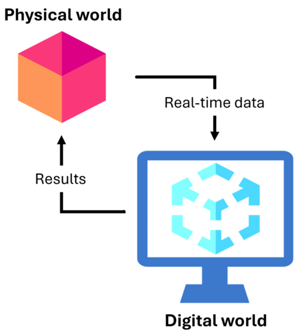
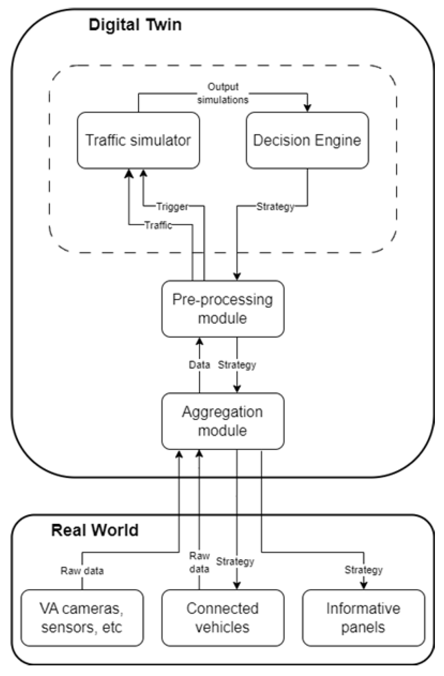
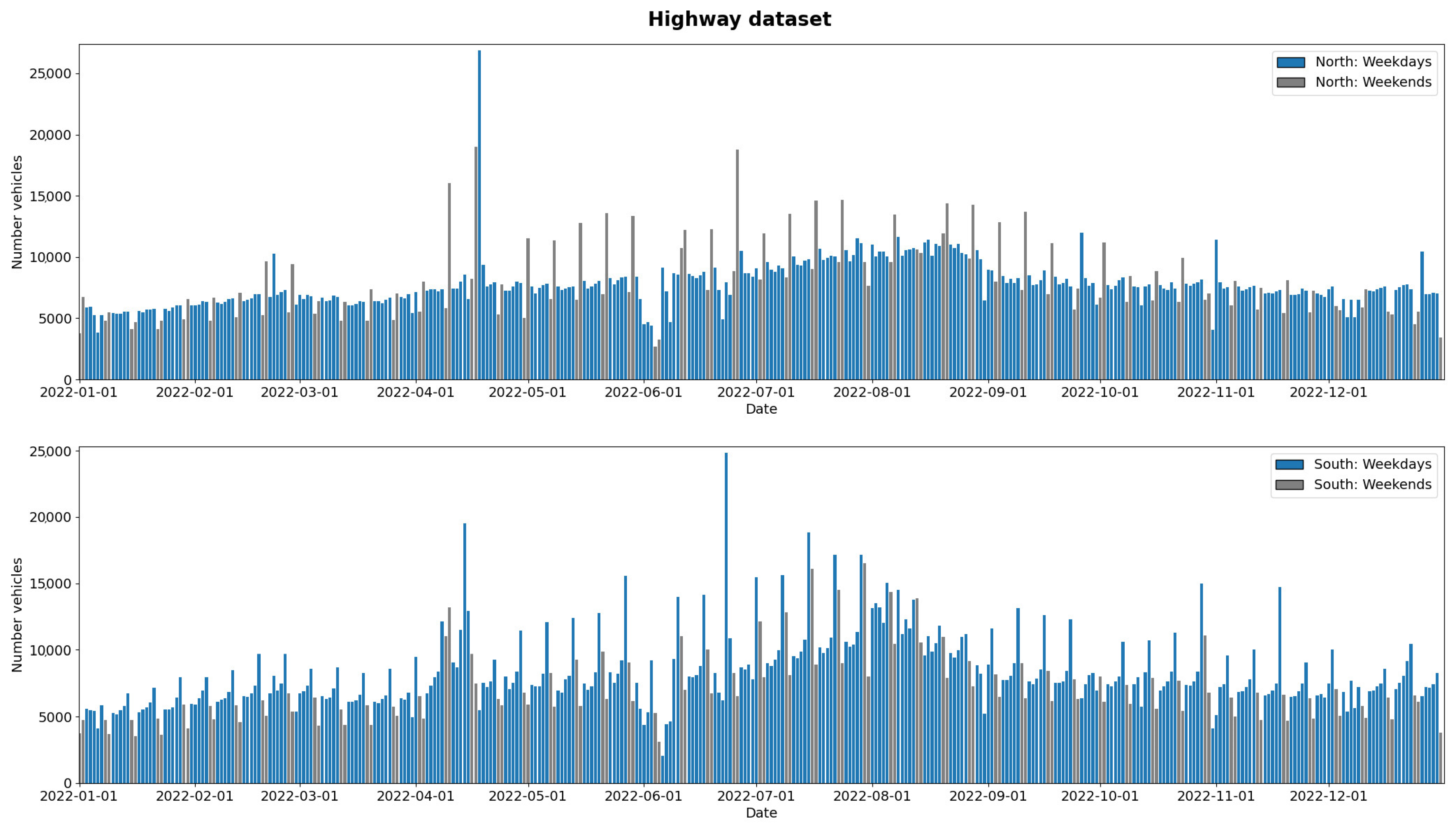


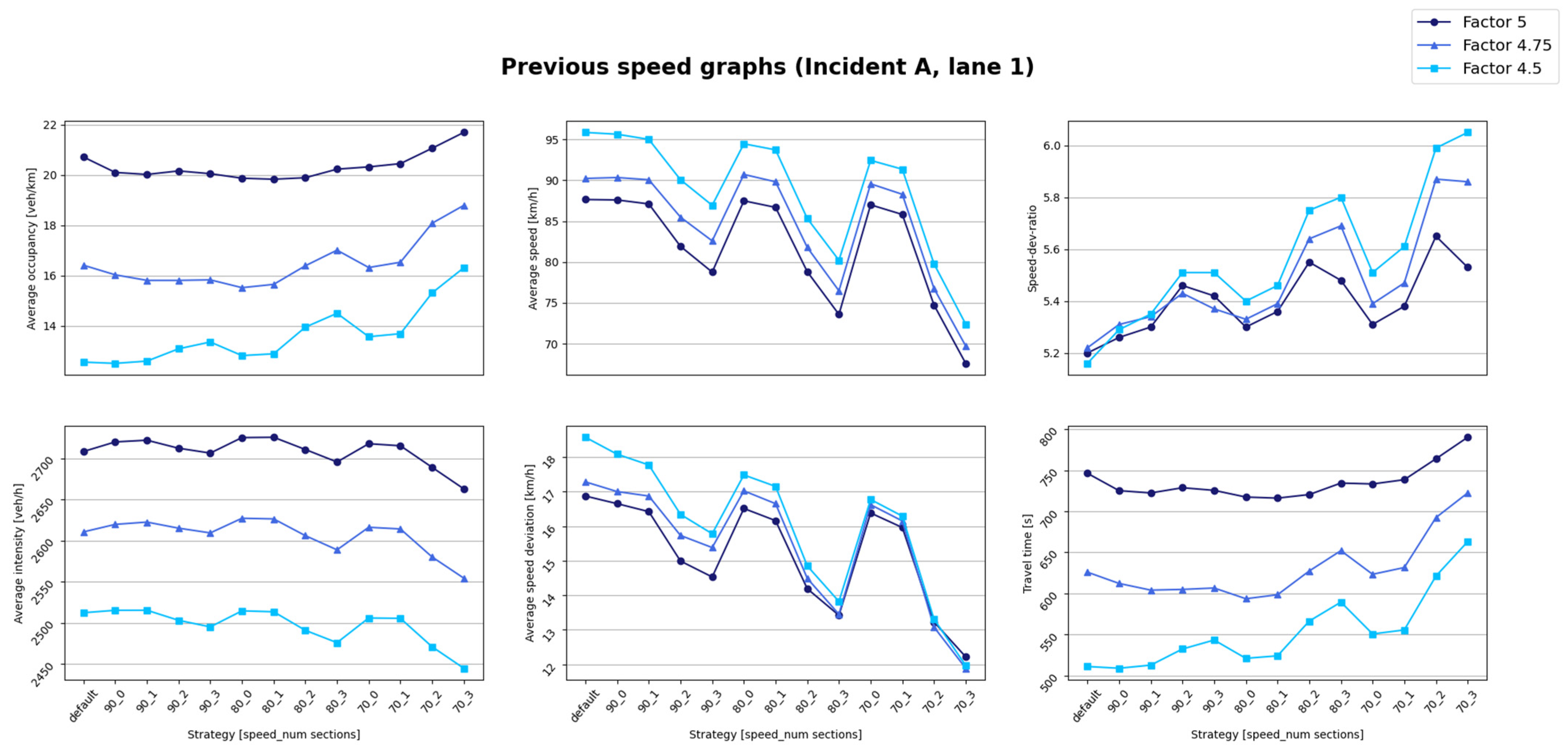

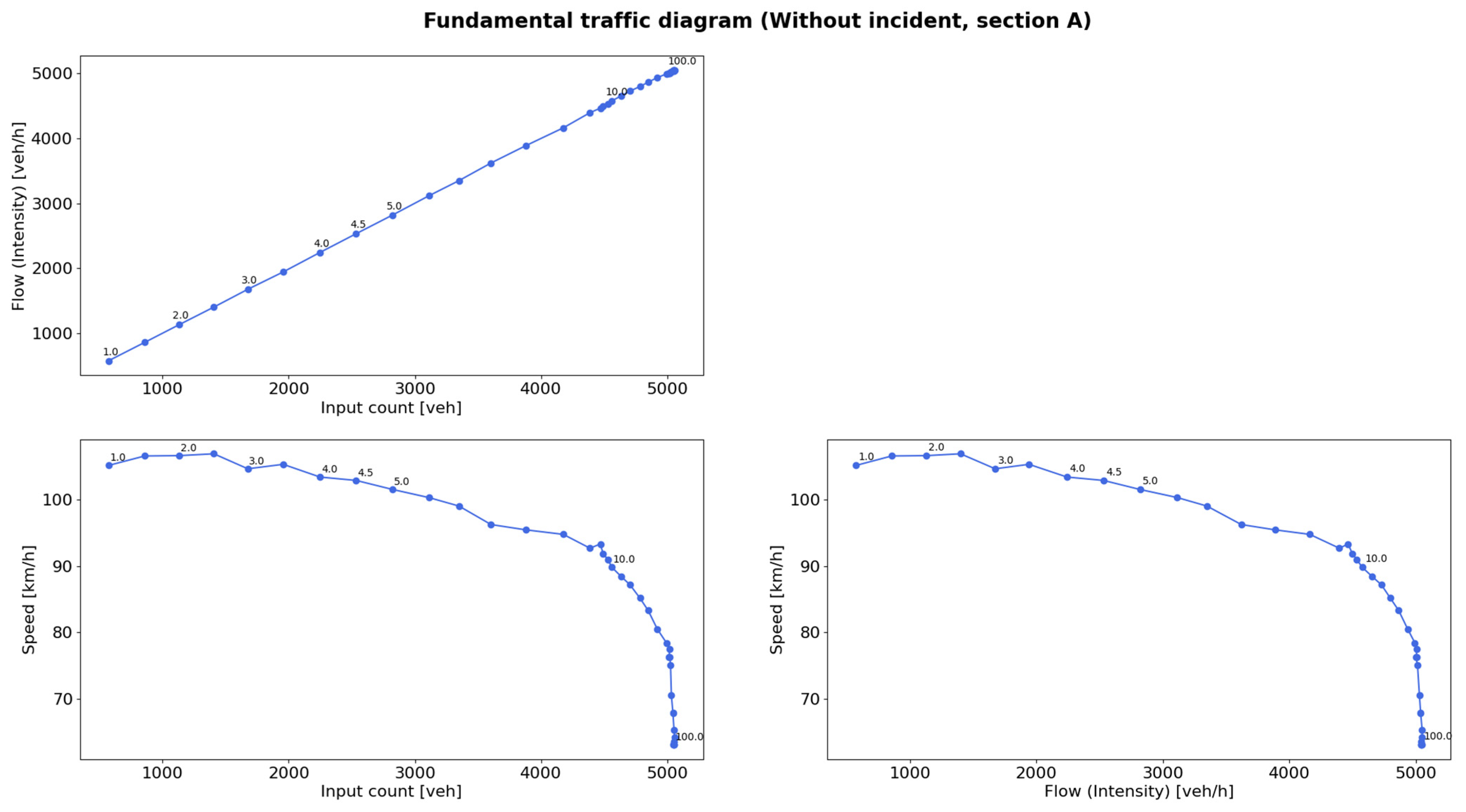


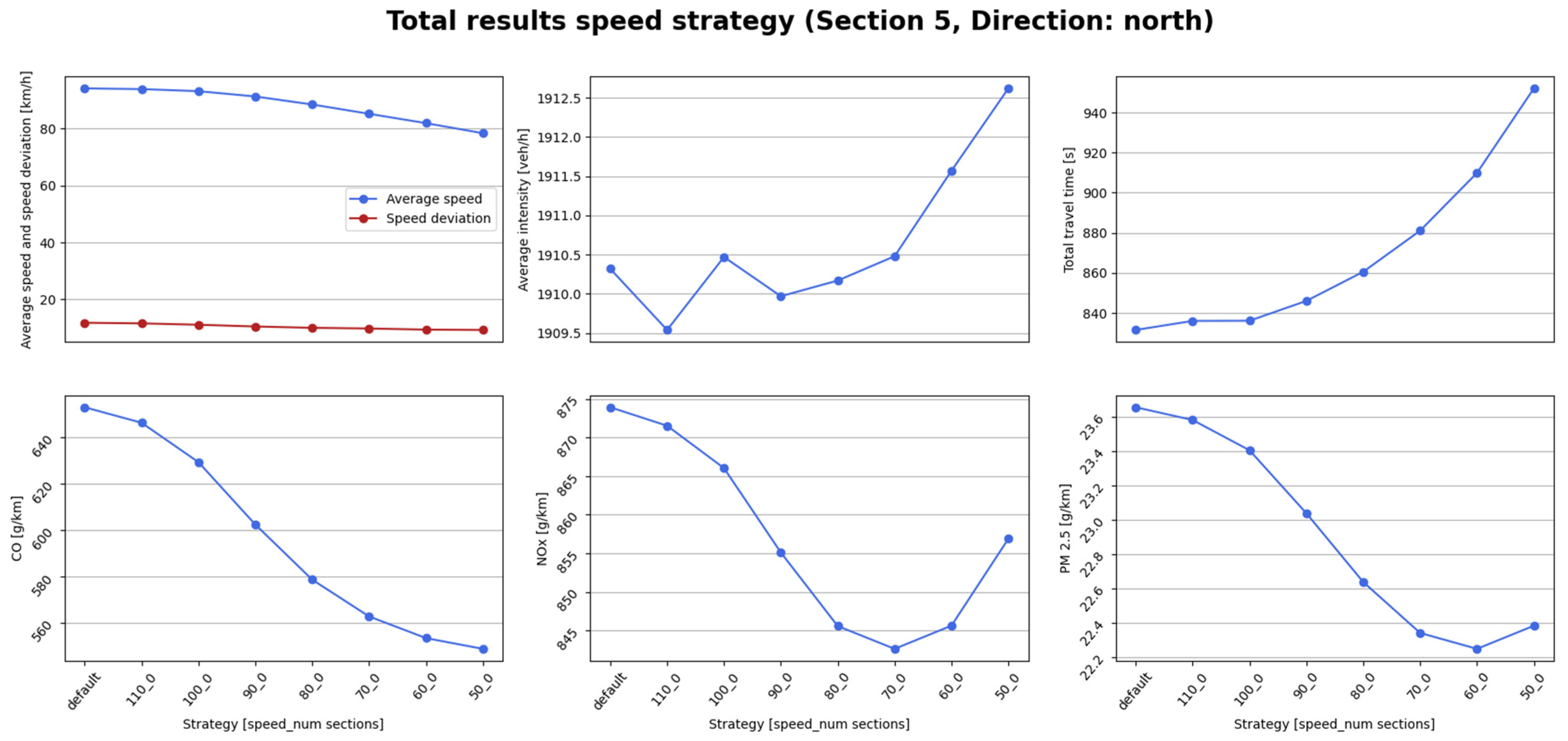
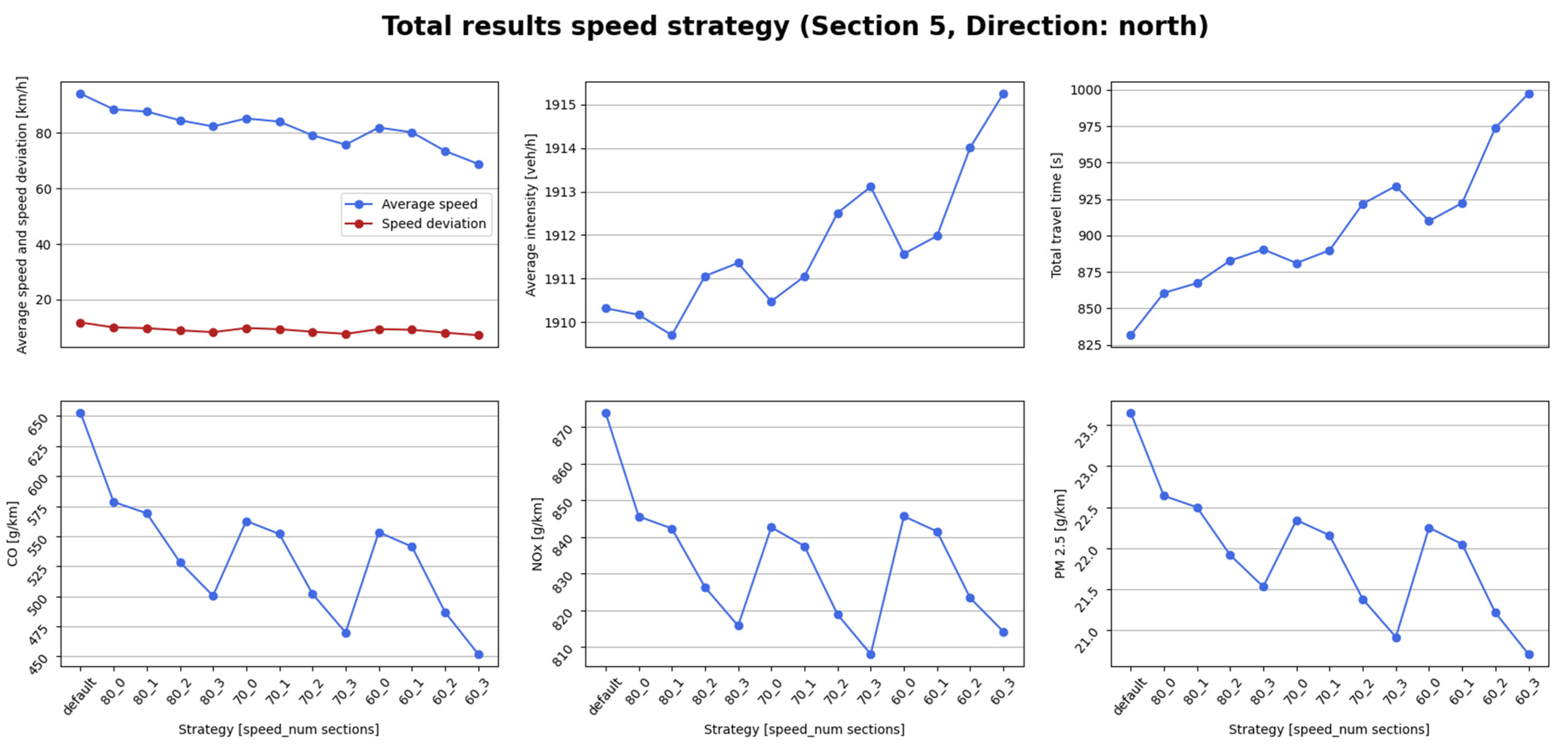
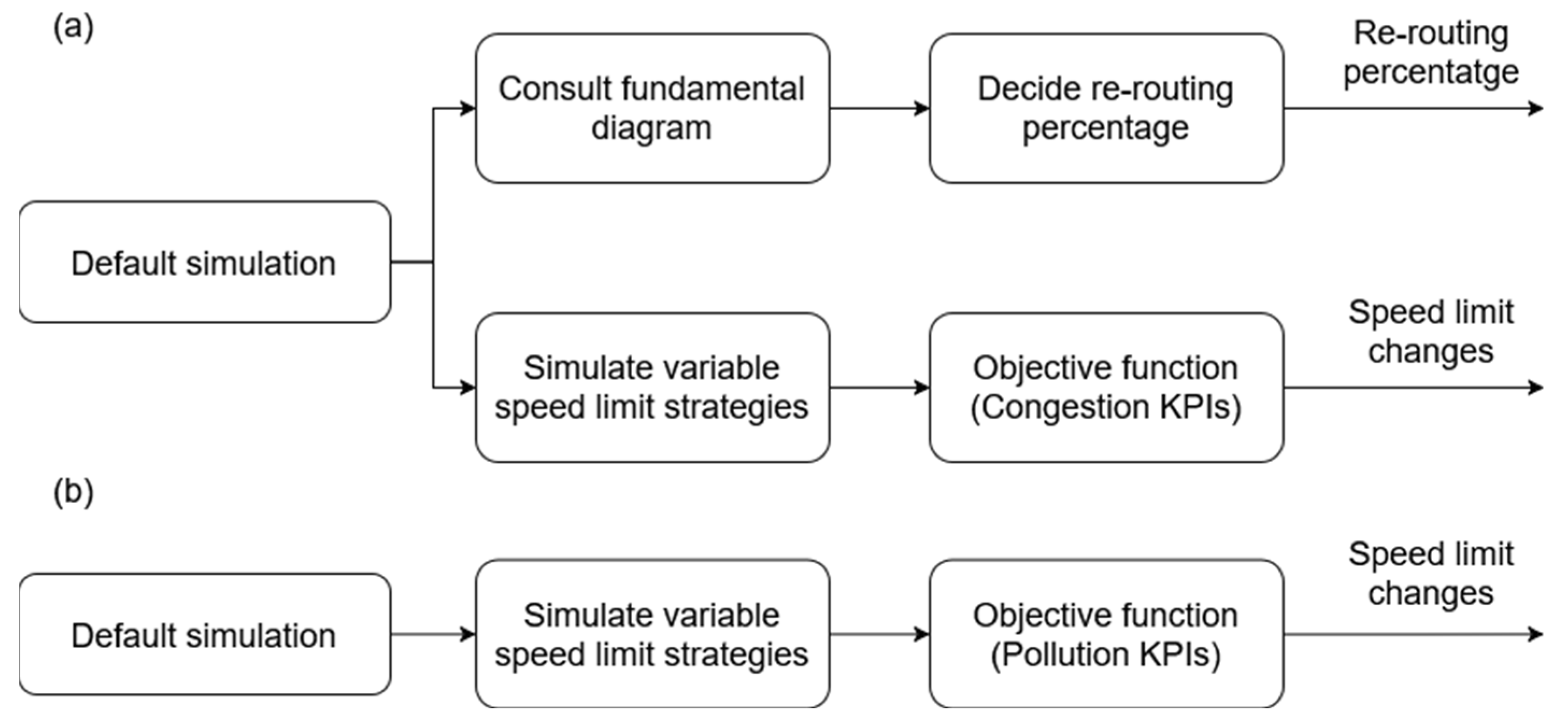
