Fluid–Structure Interaction Study in Unconventional Energy Horizontal Wells Driven by Recursive Algorithm and MPS Method

Abstract

With the unconventional energy sector (e.g., shale gas) increasingly focused on precision drilling and cost-effective extraction, slim-hole horizontal well technology is gaining prominence. However, drill string dynamics in narrow, complex fluid environments are not fully understood. This study presents a novel bidirectional fluid–structure interaction (FSI) model, uniquely integrating recursive algorithms with the Moving Particle Semi-implicit (MPS) method to couple drill string–wellbore contact with drilling fluid interactions. Key findings show that drilling fluid significantly impacts drill string behavior; for instance, it can reduce natural frequencies by 20–25%, while stiff formations amplify lateral resonance risks. Optimizing fluid properties can substantially cut energy losses, though TREE is marginally elevated when viscosity exceeds the threshold (2.5 × 10⁻⁵ m²/s). The drill string typically displaces rightward, but higher viscosity can shift it left; a moderate friction coefficient aids centering. Excessive lateral displacement impairs cuttings removal, affecting fracturing. These insights enable actionable strategies: adjusting fluid viscosity and drag reducers can optimize drill string position and enhance cleaning. This research provides a framework for energy-efficient drilling in complex reservoirs, balancing efficiency with wellbore integrity and improving outcomes in the unconventional energy sector.

1. Introduction

Driven by the demands of decarbonization and sustainable development strategies, it is foreseeable that unconventional energy sources are progressively occupying a central position in the modern energy structure [1]. One of the core aspects of promoting their application is the efficient and high-quality development of deep target reservoirs. To meet this demand, drilling technology has evolved from traditional vertical drilling to advanced horizontal well drilling and precise trajectory control techniques. Specifically, small-diameter horizontal well technology, owing to its significant advantages in enhancing drilling efficiency, reducing operational costs, achieving precise trajectory control, and expanding the effective contact area with the reservoir, has gained increasingly widespread application in the exploitation of unconventional oil and gas resources such as shale gas [2]. Indeed, the modeling of drill string dynamics in directional wells, as explored by Tengesdal et al. using Kane’s method for real-time simulation, and the analysis of nonlinear rotordynamics in curved wells by Nguyen et al., underscore the industry’s focus on these advanced drilling scenarios [3,4]. However, the prevalent phenomena of drill pipe vibration and friction during horizontal well drilling not only severely constrain drilling efficiency but also pose potential threats to operational safety. Furthermore, their impact tends to exacerbate with increasing well depth [5], representing a major contributor to tool failure, component wear, and reduced rate of penetration (ROP) [6]. This is a central concern in many studies, including the investigation of drill string–casing collision by Tchomeni Kouejou et al. and the analysis of vibrations in composite drill strings by Mohammadzadeh et al. [7,8]. Therefore, in-depth analysis, effective control, and optimization of the vibration behavior within the drill string in horizontal wells are of crucial theoretical and practical significance for ensuring efficient, safe, and economical drilling operations, as well as the efficient recovery of oil and gas resources.

Regarding drill string vibration, numerous scholars have dedicated efforts to uncovering its physical mechanisms and exploring effective vibration mitigation strategies [9]. These models range from simplified lumped-parameter approaches to complex continuous models, with Goicoechea et al. critically comparing their efficacy and highlighting the limitations of lumped models in capturing distributed phenomena like wave reflection [10]. In terms of theoretical modeling and analysis, researchers have constructed various mathematical models to characterize the complex vibration behavior of drill strings: for instance, investigating force distribution under strong vibration and optimizing drill pipe combinations by establishing a “drill string–wellbore” mechanical model [11]; deriving a lateral vibration model considering the collision effect between the drill string and the wellbore wall to analyze contact vibration characteristics and natural frequencies [12], a theme also explored by Tchomeni Kouejou et al. who modeled drill string–casing collision with a focus on rubbing damage, and by Galasso et al. who employed a penalty method for contact interactions in realistic geometries and effects of drill bit manufacturing errors and material choices on tool stress and operational safety [7,13,14]; and proposing a comprehensive vibration model incorporating axial load, drilling clearance, and contact forces to accurately analyze vibration characteristics for guiding bottom hole assembly (BHA) design [15]. The influence of BHA design and its interaction with the wellbore are critical, as emphasized by Mohammadzadeh et al. in their study of composite drill strings considering bit–rock interaction and drill string–wellbore contact, and by Tengesdal et al. who modeled BHA interactions using a component-based approach with assumed modes [8,16]. Additionally, research has also focused on suppressing specific vibration modes and energy conversion, such as active control techniques based on the concept of negative damping to suppress torsional stick–slip vibration [17]. Barjini et al. specifically designed a sliding mode controller (SMC) using an Extended Kalman Filter (EKF) to suppress coupled axial and torsional vibrations in horizontal drill strings. The challenge of stick–slip and other torsional vibrations was also a key focus for Ejike et al. in their comparative study of downscale and upscale drill strings [18,19]. Recent studies have further refined these models, such as models differentiating between drill pipes and BHA and including nonlinear bit–rock friction to analyze the influence of parameters like rotational speed and weight on bit (WOB) on torsional vibration and ROP [20]. Mohammadzadeh et al. also incorporated detailed bit–rock interaction models in their FEM analysis [8]. Concurrently, efficient and accurate modeling methods are also evolving, such as improved semi-analytical methods capable of simulating the dynamics of fluid-conveying pipelines under arbitrary geometric and boundary conditions [21]. The challenges of modeling drill strings in complex geometries like curved and directional wells are addressed by Nguyen et al. using FEM with Craig–Bampton reduction and by Tengesdal et al. using Kane’s method for real-time simulation [3,4].

The fluid–structure interaction (FSI) effect between the drilling fluid and the drill string, along with its impact on the drill string’s dynamic behavior, is a core element influencing drill string vibration and friction. Scholars often employ methods like finite element simulation and intelligent algorithms for analysis. Research areas cover the following: developing new methods for calculating the coupled modal response of flexible structures and fluids [22], and establishing governing equations for bending vibration that consider internal flow, gyroscopic effects, and external loads to fully describe the FSI field [23]. For specific systems, scholars have conducted dynamic modeling, simulation, and optimization, such as for offshore drilling riser systems and analyzing the natural frequencies of pipes containing two-phase flow [24,25]. Flow-induced instability is also a major concern, with studies analyzing the instability risk of drill strings conveying mud [26], exploring the stability of pipe columns under the combined action of internal and external flow, and particularly highlighting the dominant role of annulus flow in stability [27,28]. Tchomeni Kouejou et al. modeled hydrodynamic forces in inviscid fluid using linearized Navier–Stokes equations and explored advanced modeling of thermal and hydrodynamic conditions for specialized downhole tool deployment [7,29]. Furthermore, research has examined the influence of fluid parameters on drill string performance, revealing the complexity of friction variations under vibration and buckling conditions [30], demonstrating that adjusting drilling fluid flow rate and density can alter fluid damping and consequently affect lateral amplitude [31], and improving the accuracy of pressure loss prediction under complex conditions using neural networks [32]. The lubricating effect of drilling fluid is equally important; adding suitable lubricants can effectively reduce friction, improve force transmission, and decrease buckling risk [33,34]. Liyanarachchi and Rideout considered mud buoyancy and viscous damping in their torque and drag model [35]. Recent FSI research delves deeper, including the development of efficient 3D nonlinear finite element models for predicting stick–slip torsional vibration [36]; analyzing the stability boundaries of rotating pipes under combined internal and external flow using analytical/semi-analytical coupled models [23]; utilizing axial–torsional coupling models to analyze the different effects of feed rate and rotational speed on vibration complexity [37]; and analyzing the combined effects of mud flow rate, WOB, and rotational speed on vibration and stability through finite element models considering nonlinearities and mud effects [38]. Stability analysis under fluctuating loads also indicates that fluctuating WOB and related parameters can drive parametric resonance instability [39].

The rheology of existing drilling fluids has limited effectiveness in suppressing vertical chatter, and their shear-thinning behavior may conflict with vibration damping requirements [40]. Volpi et al. specifically modeled non-Newtonian fluids using the Quemada model to assess their impact on hydraulic forces [41]. However, considering the dynamic pressure drop of non-Newtonian fluids significantly alters the predicted critical rotational speeds for lateral vibration, especially under specific operating conditions, suggesting this factor should be included when formulating vibration avoidance strategies [42]. Further research indicates that the optimal combination of drilling fluid rheological parameters differs for suppressing different types of vibration (axial, lateral, torsional), providing a theoretical basis for vibration control through drilling fluid optimization [43].

The frictional energy dissipation between the drill string and wellbore wall, as a non-productive energy expenditure, should be minimized during the drilling process. However, related research is scarce. Simultaneously, many analyses tend to simplify the drill string as a slender rotating beam, which, to some extent, neglecting its complex three-dimensional structural dynamic characteristics. This simplification is challenged by models like those from Galasso et al., which use geometrically exact rod theory, and Nguyen et al., who employ 3D beam finite elements for curved wells. Goicoechea et al. also emphasized that drill strings are inherently distributed systems and simple lumped models fail to capture their rich dynamics [4,10,13]. Furthermore, in-depth research remains insufficient regarding the highly nonlinear, two-way fluid–structure coupling problem under transient conditions, particularly in scenarios involving small-diameter horizontal wells where drill string–wellbore contact friction is more severe, and the gravitational and hydrodynamic effects of the drilling fluid are more pronounced. Traditional added mass and damping methods struggle to fully capture the complex coupled dynamic behavior. This is a gap that Volpi et al.’s LBM-FEM approach aims to address by directly simulating the fluid dynamics and their interaction with the structure [44].

In view of this, the present study focuses on establishing effective numerical models to describe the dynamics of small-diameter horizontal drill strings and the two-way fluid–structure coupling effect. A recursive algorithm is employed for transient dynamics analysis, combined with the advanced Moving Particle Semi-implicit (MPS) method, to analyze the vibration response, frictional energy consumption, and flow field characteristics, thereby providing theoretical support and optimization guidance for the safe and efficient drilling of small-diameter horizontal wells.

2. Bidirectional FSI Numerical Model

2.1. Dynamic Modeling

2.1.1. Multi-Body Model

The drill string composed of multi-sectional drill pipes can be regarded as a flexible multi-body system. The system is first discretized using the finite element method, and topological relationships are established to define inter-element connections. The discretized system is represented by simplified point–line relationships between nodes and elements. Dedicated local coordinate systems are established at the centroids of each flexible and rigid body, while the global coordinate system is positioned at the bottom hole center. The generalized coordinate set of the system is given by Equation (1) [45].

$$q=\left[\begin{array}{c}{q}_r\\ q_e\end{array}\right]$$

(1)

where q_r represents the rigid body degrees of freedom, and q_e denotes the flexible body degrees of freedom.

During analysis, forward and backward recursions are employed to solve kinematics and dynamics, respectively. The forward recursion initiates from the load-application end of the drill string borehole, serving as the base body. This process encompasses velocity, acceleration propagation for rigid bodies, and deformation superposition for flexible bodies. The recursion of rigid-body velocity and acceleration are formulated in Equation (2) and Equation (3) [46], while flexible-body elastic deformation displacements are computed via Equation (4) [47].

$$v_i=v_{i-1}+J_i^{\mathrm{joint}}{\dot{q}}_i+{\beta }_i$$

(2)

$$a_i=a_{i-1}+J_i^{\mathrm{joint}}{\ddot{q}}_i+{\gamma }_i$$

(3)

$${\dot{u}}_i=N_i{\dot{q}}_{e,i}$$

(4)

Here, J_i^joint denotes the Jacobian matrix, γ_i represents the Coriolis and centrifugal terms, and N_i corresponds to the shape function matrix.

During backward recursion, the resultant force of each body and the force transmitted to the parent body are individually formulated as shown in Equations (5) and (6) [46,47].

$$f_i=M_i{a}_i^{\mathrm{total}}+C_i{v}_i^{\mathrm{total}}+K_i{u}_i-f_{\mathrm{ext},i}$$

(5)

$$f_{i-1}=f_i+J_i^{\mathrm{joint},T}{\tau }_i$$

(6)

where f_ext,i denotes the external force, and τ_i represents the driving force.

The dynamic equation of the system can be expressed as shown in Equation (7) [48,49].

$$\left\{\begin{array}{l}M(q)\ddot{q}+C(q,\dot{q})+Kq=Q_{ext}+Q_c\\ \Phi (q,t)=0\end{array}\right.$$

(7)

where M denotes the mass matrix, and Φ represents the constraint equations.

To ensure that the connection constraints between all bodies in a multi-body system are strictly satisfied during its motion, the Lagrange multiplier method is employed to address the constraints, with the augmented equations formulated as shown in Equation (8) [50].

$$\left[\begin{array}{cc}M& {\Phi }_{\mathrm{q}}^T\\ {\Phi }_{\mathrm{q}}& 0\end{array}\right]\left[\begin{array}{c}\ddot{q}\\ \lambda \end{array}\right]=\left[\begin{array}{c}Q\\ -{\Phi }_t-{\Phi }_{\mathrm{q}}\dot{q}\end{array}\right]$$

(8)

Here, Φ_q denotes the Jacobian matrix associated with the constraint equations.

Furthermore, the recursive resolution of drill string dynamics is accomplished through iterative updates of generalized coordinates and velocities.

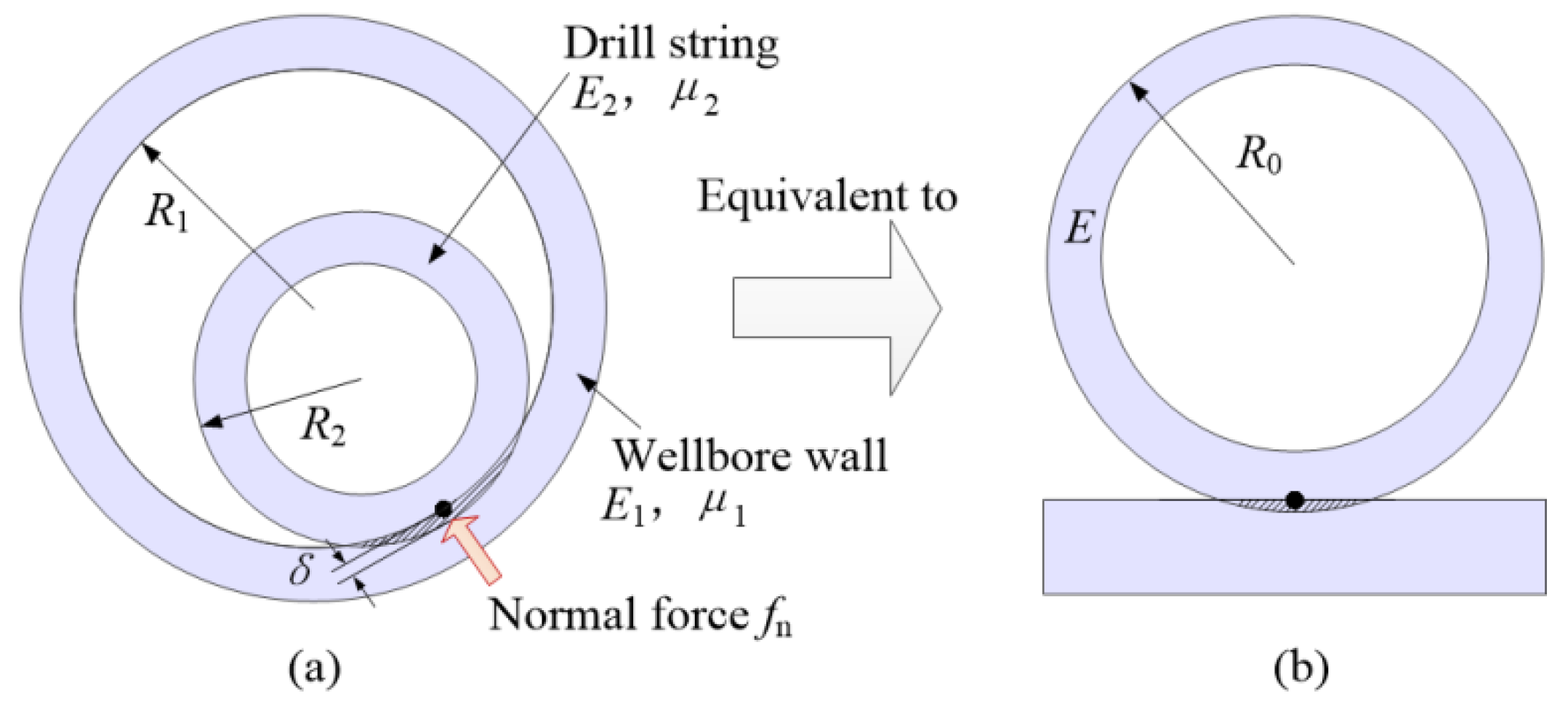
2.1.2. Drill String–Wellbore Wall Contact Force

The contact relationship between the drill string and wellbore wall, as illustrated in Figure 1a, represents an internal contact with strong nonlinearity. Based on the contact radius relationship within the contact area, the contact between the drill string and borehole wall can be equivalently simplified as the contact between a cylindrical object with an equivalent radius R₀ and a flat surface, as shown in Figure 1b. The correlation used to determine this equivalent radius R₀ is expressed as Equation (9) [51].

$${\displaystyle \frac{1}{R_0}}={\displaystyle \frac{1}{R_2}}-{\displaystyle \frac{1}{R_1}}$$

(9)

where R₁ denotes the curvature radius of the wellbore (concave surface) and R₂ represents the curvature radius of the drill pipe (convex surface). In this study, the drill string outer diameter is 71 mm (thus, R₂ = 35.5 mm), and the wellbore inner diameter is 76 mm (thus, R₁ = 38 mm). Substituting these values into Equation (9), the equivalent contact radius R0 is calculated to be 539.6 mm. According to the Hertzian contact theory, it is assumed that mutual interpenetration occurs between two contacting bodies under applied loads, and the contact forces between contacting bodies can be derived using the generalized Hooke’s law and the stress–strain relationships of materials.

To facilitate the derivation of the governing equations, a representative example—the contact problem of two elastic spheres with different diameters—is employed in the subsequent analysis. After establishing the generalized contact force formula, the equivalent contact radius between the drill string and the wellbore wall will be substituted into the final expression.

As shown in Figure 2, the geometric relationships within the contact area are defined under the assumption that mutual indentation occurs due to the applied load. Sphere A and sphere B have respective initial (undeformed) radii of curvature R₁ and R₂. The x-y plane, serving as the reference plane, is defined as the plane passing through the center O of the circular contact area. The radius of the contact area is a. The total indentation depth δ represents the total relative displacement by which the two spheres approach each other along the z-axis from their initial state of tangential contact. δ is the sum of the indentation δ₁ of sphere A and δ₂ of sphere B (i.e., δ = δ₁ + δ₂). At r = a, z₁ is the normal distance from a point on the undeformed surface of sphere A to its original vertex tangent plane. Similarly, z₂ is the corresponding sagitta (profile height) for sphere B at r = a. w₁ and w₂ denote the normal distances from points on the deformed surfaces of sphere A and sphere B, respectively, at the radial distance r = a, to the common x-y plane. Their sum represents the normal gap between the two deformed surfaces at the edge of the contact radius a. Based on these geometric definitions, the relationship among the parameters w₁, w₂, z₁, z₂, and δ at r = a is given by Equation (10). Thus, a quantitative relationship is established for the gap (w₁ + w₂) between the two deformed bodies at the edge of the contact area (r = a), the total indentation depth δ, and the initial geometric parameters of the contacting bodies.

$$w_1+w_2=\delta -(z_1-z_2)$$

(10)

The equivalent contact radius and equivalent elastic modulus of the two contacting bodies are formulated in Equation (11) [52,53]. According to the Hertzian theory, the pressure distribution across the contact surface is semi-ellipsoidal, with the total load denoted as Q. The relationships among the penetration depth, contact radius, and contact pressure can be determined through integral relationships, as shown in Equation (12) [54].

$$\left\{\begin{array}{l}R={\displaystyle \frac{R_1{R}_2}{R_1+R_2}}\\ E={\displaystyle \frac{E_1{E}_2}{E_2(1-{\mu }_1)+E_1(1-{\mu }_2)}}\end{array}\right.$$

(11)

$$\left\{\begin{array}{l}{q}_{\max }={\displaystyle \frac{3Q}{2\pi }}({\displaystyle \frac{4}{3Q\pi (l_1+l_2)R}}{)}^{{\displaystyle \frac{2}{3}}}\\ a^3={\displaystyle \frac{3Q\pi (l_1+l_2)R}{4}}\\ {\delta }^3={\displaystyle \frac{9Q^2{\pi }^2{(l_1+l_2)}^2}{16R}}\end{array}\right.$$

(12)

where q_max is the maximum pressure at the contact center, and l₁ and l₂ can be represented by Equation (13) [55].

$$l_1={\displaystyle \frac{1-{{\mu }_1}^2}{\pi E_1}},l_2={\displaystyle \frac{1-{{\mu }_2}^2}{\pi E_2}}$$

(13)

Ultimately, the general form of the contact force can be expressed as shown in Equation (14).

$$F=K·{\delta }^{1.5}$$

(14)

where K represents the stiffness coefficient, which is determined by the material properties of the contacting bodies and the equivalent contact radius, and can be expressed by Equation (15) [56]:

$$K=\sqrt{{\displaystyle \frac{16R{E}^2}{9}}}$$

(15)

The normal contact force between the drill string and the wellbore wall consists of the stiffness force and the damping force. The normal contact force can be calculated by Equation (16) [57].

$$f_n=f_{ns}+f_{nd}=K{\delta }^{1.5}+C{\displaystyle \frac{\dot{\delta }}{\left|\dot{\delta }\right|}}{\left|\dot{\delta }\right|}^{m1}{\delta }^{m2}$$

(16)

where K is the stiffness coefficient, C is the damping coefficient, $\dot{\delta }$ is the time derivative of δ, m₁ is the nonlinear contact force index, and the index m₂ produces the indentation damping effect. In this study, the values of m₁ and m₂ are taken as 1 and 2, respectively.

2.2. Fluid Domain Solution

2.2.1. MPS Method

Numerical modeling of fluid domains using conventional Eulerian frameworks often requires continuous grid reinitialization, which becomes computationally unstable when handling strong nonlinear interfacial interactions and substantial structural deformations. Conversely, Lagrangian-based approaches monitor discrete fluid particle trajectories, inherently ensuring rigorous conservation of mass and momentum—a critical advantage for domains with evolving boundaries. To address the bidirectional FSI between the drill string and drilling fluid, this research adopts the Moving Particle Semi-implicit (MPS) methodology [58,59], a particle-centric Lagrangian technique that circumvents grid dependency through adaptive particle discretization and robustly resolves extreme deformation scenarios.

Assuming that the drilling fluid is incompressible, the spatial fluid is discretized into a finite number of particles with basic physical quantities such as pressure, velocity, and mass. Based on the conservation of mass and momentum, the governing equations in Lagrangian form for the fluid domain can be expressed by Equation (17) [60].

$$\left\{\begin{array}{l}{\displaystyle \frac{D\rho }{Dt}}=0\\ {\displaystyle \frac{Du}{Dt}}=-{\displaystyle \frac{\nabla P}{\rho }}+v{\nabla }^{2}u+g\end{array}\right.$$

(17)

where ρ is the density of the drilling fluid, u is the displacement, v is the velocity, and g is the gravitational acceleration.

The interaction between particles is calculated using the weighting function. It is unrealistic to calculate the interaction forces between all particles in the entire drilling fluid domain, and the actual influence between two particles that are far enough apart can be ignored. Therefore, the effective calculation radius of the particles is set as r_e, as shown in Figure 3. The interaction forces are calculated only within r_e. Those beyond the scope will not be considered.

The pressure correction of the governing equation is solved implicitly. During discretization, the pressure gradient term is approximated using inter-particle pressure differences among drilling fluid particles, whose formulation is given by Equation (18) [60].

$${〈\nabla P〉}_i={\displaystyle \frac{d}{n_0}}{\displaystyle \sum _{i\ne j}\left[\frac{P_j-P_i(r_j-r_i)}{r_j-r_i\left|r_j-r_i\right|}W(\left|r_j-r_i\right|)\right]}$$

(18)

where W(|r_j − r_i|) is a weighting function, which is used to measure the interaction force between particles.

For explicit computation of the viscous and external force terms, the Laplacian operator acting on the velocity difference of particle i relative to its neighbors is discretized into the form shown in Equation (19) [61].

$${〈{\nabla }^{2}u〉}_i={\displaystyle \frac{2d}{\lambda n_0}}{\displaystyle \sum _{j\ne i}(u_j-u_i)}W(\left|r_j-r_i\right|)$$

(19)

Here, d represents the spatial dimension, and λ can be expressed as

$$\lambda ={\displaystyle \frac{{\displaystyle \sum _{j\ne i}{\left|r_j-r_i\right|}^2}W(\left|r_j-r_i\right|)}{{\displaystyle \sum _{j\ne i}W(\left|r_j-r_i\right|)}}}$$

(20)

For the basic solution process of time integration, the MPS method couples explicit and implicit solution strategies. Firstly, the velocity field is predicted through explicit calculation, as shown in Equation (21) [58]. Then, the pressure field is solved through an implicit algorithm, and the update and correction of the velocity field are completed simultaneously. The updated form can be expressed as shown in Equation (22) [58].

$$u^{*}=u^n+\Delta t(v{\nabla }^2{u}^n+g)$$

(21)

$$u^{n+1}=u^{*}-{\displaystyle \frac{\Delta t}{\rho }}\nabla P^{n+1}$$

(22)

where u* represents the prediction of the velocity field, uⁿ⁺¹ is the updated and corrected velocity field, and ∆t represents the time step.

2.2.2. Boundary Conditions

The inner and outer diameters of the drill string are 61 mm and 71 mm, respectively, and the diameter of the wellbore is 76 mm. The coupling relationships include the drill string–internal fluid coupling and the drill string–annular fluid coupling. The particle size of the fluid can have a significant impact on the analysis results. In order to balance the analysis accuracy and the solution speed, the relationship between the particle size and the total wall pressure was explored. The density of the drilling fluid is 1000 kg/m³, the kinematic viscosity is 1 × 10⁻⁶ m²/s, and the flow rate is 50 L/min. The total pressure of the fluid domain mapped to the inner wall surface of the drill string within a 1000 mm long section is shown in Figure 4. When the particle size is less than 4 mm, the total pressure fluctuation of the drill string wall is small, and the total pressure of the wall corresponding to 4 mm is approximately 3.5% different from that in the case of 1 mm. However, when the size is greater than 4 mm, the total wall pressure increases sharply; at this point, due to the larger particle dimensions, the particle geometry penetrates the drill string wall during contact, resulting in significantly higher wall forces exerted on the drill string. Comprehensively considering the solution accuracy and speed, the particle size is set to 4 mm.

The drill string and wellbore wall models are shown in the Figure 5. In order to enable the particles to pass through the annular gap, the particles in the annular gap are refined, and the size of the refined particles is 0.3 mm. To improve the solution efficiency, the internal fluid and annular fluid are solved, respectively. The schematic diagram of the coupling model is shown in Figure 6.

2.3. Bidirectional FSI Algorithm

The multi-body dynamics theory was combined with the MPS theory to construct a bidirectional transient solid–liquid coupling model. During the model construction process, both the contact between the drill string and the wellbore wall and the FSI effects are considered simultaneously. The fluid domain and the structure domain achieve data exchange through their contact interface. The structure of the drill string mainly affects the drilling fluid through displacement and velocity, while the drilling fluid is mainly applied to the wall surface of the drill string in the form of wall force. The bidirectional coupling process is shown in Figure 7 and can be divided into the following steps:

Step 1: Solve the structural domain (drill string) and fluid domain (drilling fluid) at time step t(i). Transfer the fluid-induced wall forces and torque calculated from the fluid domain to the corresponding structural boundaries as external loads.

Step 2: Update the drill string configuration by solving the structural dynamics under applied fluid loads, obtaining nodal displacements and velocities at t(i + 1).

Step 3: Archive the updated structural parameters (positions, velocities) at t(i + 1) for subsequent coupling iterations.

Step 4: Propagate the t(i + 1) structural boundary conditions (positions, velocities) to the fluid domain to redefine moving interfaces.

Step 5: Advance the fluid domain transient simulation to t(i + 1) using the updated structural boundary data.

Step 6: Recalculate fluid-induced forces (pressure, shear) at the fluid–structure interface for t(i + 1).

Step 7: Map the recalculated fluid loads (forces, torque) to the structural domain as boundary conditions for the next time step.

Step 8: Iterate Steps 1–7 until convergence or terminal simulation time.

2.4. Experiments and Validation

2.4.1. Experimental Setup

An indoor simulated drilling experiment platform was developed based on similarity theory. The experimental system comprises a drive module, drill string module, borehole-bottom module, data acquisition and processing module, and drilling fluid circulation pipelines, as illustrated in Figure 8a. Considering the favorable physical property similarity between acrylonitrile-butadiene-styrene (ABS) and actual drill strings, an ABS pipe with an inner diameter of 26 mm and an outer diameter of 32 mm was selected as the simulated drill pipe. Transparent acrylic glass with an inner diameter of 35 mm was employed for the borehole wall to facilitate observation and machining. The dimensional correspondence between the simulated drill string, wellbore wall, and actual parameters is presented in the

Table 1. Dimensional correspondence between the simulated drill string and wellbore wall and actual parameters.

Parameter	Drill String		Wellbore Wall
	Actual Value	Simulated Value	Actual Value	Simulated Value
Young’s modulus (GPa)	205	2.2	55	2.6
Poisson’s ratio	0.29	0.394	0.26	0.35
Density (kg/m3)	7850	1100	2600	1180

. The total length of the simulated drill string is 5650 mm. This platform enables adjustable control of key parameters including feed pressure, rotational speed, and drilling fluid flow rate. As shown in Figure 8b, the data acquisition system integrates multiple sensors for real-time measurement. Acquired signals are converted and transmitted to a computer via the RS485 communication protocol, with independently developed MATLAB-based software (R2025a (v25.1)) performing integrated analysis.

To eliminate the additional frictional torque consumption caused by the friction of dynamic sealing components at both ends of the drill string, a no-load baseline experiment was conducted (feed pressure 0 N, flow rate 0 L/min, rotational speed 256 rpm). The driving torque was measured to be 0.46 N·m at this time. This value was added as an initial boundary condition to the simulated kinematic pair. Simultaneously, the friction coefficients measured in the laboratory between the drill string and the wellbore wall, and between the drill bit and the bottom hole, were 0.3621 and 0.3529, respectively. These were used to calibrate the simulation model.

2.4.2. Validation

The numerical model was experimentally validated using an indoor simulated drilling platform. Figure 9 demonstrates the variation trend of driving torque with feed pressure. It can be observed that the experimental and simulated values of driving torque exhibit similar patterns, with the driving torque increasing as feed pressure rises. The maximum error of approximately 12.98% occurs at a feed pressure of 15 N, which can be attributed to the fact that the majority of the driving force is predominantly consumed in overcoming frictional resistance induced by manufacturing tolerances within the experimental setup.

Figure 10 illustrates the variation trend of annular outlet velocity with the flow rate of drilling fluid in the wellbore. It can be seen that the experimental values and the simulated values have a high similarity, with a maximum error of approximately 6.87%, indicating that the model has a high accuracy.

Figure 11 illustrates the centroid trajectory at the midpoint of the drill string. The experimental and simulated values exhibit good agreement in motion trajectories and share the same trend, with the drill string primarily moving in the lower-right region of the wellbore. At higher rotational speeds, the simulated errors increase significantly. This indicates that when the rotational speed increases, the movement amplitude of the drill string increases while the randomness of the movement gradually increases.

To further validate the high efficiency of the recursive algorithm adopted in this paper, a comparison was made with a typical explicit dynamics analysis method (LS-DYNA). The hardware specifications used in this study were an Intel Core i7-14700KF CPU, an NVIDIA GeForce RTX 4090 graphics card, and 64 GB of RAM. The benchmark case used for this comparison was a drill string model with a total length of 20 m, simulated for a physical time of 3 s. The relevant comparison results are shown in

Table 2. Cost comparison of two solution methods.

Condition	Parameter	Explicit Dynamics	Recursive Algorithm	Efficiency Improvement (vs. Explicit Dynamics)
Condition 1	Mesh Size (mm)	1.8	1.8	59.3%
	Element Count	422,682	356,520
	Total Sim. Time (Days)	4.3	1.75
Condition 2	Mesh Size (mm)	8	8	56.3%
	Element Count	132,400	124,800
	Total Sim. Time (Days)	0.96	0.42

. Comparative analysis demonstrates that the recursive algorithm employed in this study exhibits a significant computational efficiency advantage in solving drill-string dynamics with nonlinear contact. It substantially reduces computational time; for instance, under a mesh size of 1.8 mm, the recursive algorithm reduces the computational time by approximately 59.3% compared to conventional explicit methods.

In summary, systematic validation has thoroughly confirmed the effectiveness, accuracy, and significant computational advantages of the bidirectional FSI numerical model and its integrated recursive algorithm developed in this study.

3. Results and Discussion

3.1. Dynamic Response Under Drilling Parameters

As illustrated in Figure 12, three tracer particles were selected within the drill string fluid to analyze their trajectories over a 1 s timeframe. The particle motion paths under different drilling parameters are depicted in Figure 13. Driven by drill string rotation and centrifugal forces, the fluid exhibits helical flow patterns, with particles at different radial positions demonstrating motion independence—indicating negligible radial interference. Notably, particles closer to the drill string axis (Particle 1) experience reduced rotational and centrifugal effects, exhibiting prolonged rotational periods and elongated axial pitch. Specifically, the rotational periods in Figure 13a are 0.18 s, 0.24 s, and 0.25 s; in Figure 13b, 0.15 s, 0.20 s, and 0.21 s; and in Figure 13c, 0.10 s, 0.15 s, and 0.17 s. These results demonstrate a radial gradient in rotational influence, with periods lengthening from the wall toward the center. Elevating the rotational speed or axial flow rate effectively accelerates helical flow velocities.

Figure 14 shows the effect of drill string internal fluid on the drill string under different rotational speeds. The average contact force between the drill string and wellbore wall increases with rotational speed, exhibiting a 9.65% rise at 800 rpm compared to static conditions (0 rpm). Under combined gravitational and rotational coupling, sustained contact predominantly localizes in the lower-right quadrant, while elevated centrifugal loading degrades stability and intensifies collision frequency at higher speeds. Additionally, the centrifugal force-induced radial pressure gradient within the fluid intensifies with increasing rotational speed, consequently amplifying the wall forces exerted on the drill string.

Figure 15 shows the effect of drill string internal fluid on the drill string under varying feed pressures. The increase in feed pressure exacerbates the deformation-induced squeezing of the drill string against the borehole wall, leading to a corresponding increase in average contact force. The average contact force exhibits an 8.4% elevation at 15 kN feed pressure relative to the zero-load condition. However, the elevated feed pressure does not directly affect the internal fluid dynamics, and there was no obvious increasing trend of the wall force of the fluid on the drill string.

Regarding the annular fluid, Figure 16 illustrates the effect of varying rotational speeds on the drill string. An increase in rotational speed enhances the hydrodynamic pressure effect of the annular fluid on the drill string. The intensified hydrodynamic pressure reduces contact between the drill string and borehole wall, while the wall force exerted by the fluid on the drill string increases concurrently.

Figure 17 shows the influence of annular fluid on the drill string under different feed pressures. Although the increase in feed pressure will intensify the squeezing between the drill string and the wellbore wall, it has no effect on the wall force of the fluid.

Figure 18 clearly reveals the significant influence of different rotational speeds (400 rpm, 600 rpm, and 800 rpm) on the annular velocity field distribution under conditions of constant drilling fluid parameters: a flow rate of 50 L/min, a kinematic viscosity of 1 × 10⁻⁶ m²/s, and a density of 1000 kg/m³. Due to the eccentric positioning of the drill string within the wellbore (located in the lower-right region of the annulus), a narrow annular gap is formed between the drill string and the wellbore wall in this area. Observational results indicate a highly non-uniform fluid velocity distribution within the annulus. Specifically, in the narrow annular region of the lower-right, due to eccentricity, a distinct high-velocity zone is formed owing to the strong shearing and dragging action of the rotating drill string (i.e., mechanical disturbance); this high velocity is attributed to the acceleration effect on the fluid within the narrow channel and the direct momentum transfer from the rotating drill string.

Critically, as the drill string’s rotational speed increases (from 400 rpm to 800 rpm), this high-velocity zone not only expands significantly in the circumferential direction but also experiences an evident increase in its internal fluid velocity magnitude (e.g., at 800 rpm, the area covered by orange and red, representing higher velocities in the lower-right region, is considerably larger than at 400 rpm, with velocities approaching 3.0 m/s). The expansion and velocity intensification of this high-velocity zone are crucial for the efficient transport of cuttings in horizontal wells, significantly enhancing cuttings carrying capacity and improving wellbore cleanliness. This, in turn, optimizes subsequent hydraulic fracturing efficiency by reducing flow resistance and minimizing formation damage. Concurrently, given the relatively narrow annular clearance and the low kinematic viscosity of the drilling fluid, the fluid flow is predominantly characterized by circumferential and axial components, resulting in an insignificant radial velocity gradient.

Figure 19 investigates the effect of different feed pressures (10, 13, and 15 kN) on the annular velocity field at a specific rotational speed and with the same drilling fluid parameters as in Figure 18. The results clearly indicate that despite an increase in feed pressure, the overall distribution of the annular velocity field—including the morphology, location, and velocity magnitude of the high-velocity zone—exhibits no significant changes. This demonstrates that the flow field characteristics are insensitive to variations in feed pressure. This insensitivity is presumably because the macroscopic annular flow field is primarily governed by hydrodynamic factors such as drill string rotation and drilling fluid circulation rate, whose effects substantially outweigh minor perturbations to local contact conditions from feed pressure changes. Concurrently, under the drill string parameters of this study (a length of 20 m), variations in feed pressure are unlikely to cause significant alterations in the drill string’s macroscopic posture or the annular geometry, and the associated energy may be dissipated through other mechanical interactions (such as drill bit–rock interaction). Therefore, feed pressure has a minor impact on the main annular velocity distribution, a finding relevant for optimizing drilling parameters.

3.2. Impact of Drilling Fluid

3.2.1. Drill String Vibration Response

The drilling fluid inside the drill string significantly influences its vibration characteristics, while the supporting effect of the wellbore alters the boundary conditions of the drill string. The upper end of the drill string at the wellhead is set as a fixed constraint, and radial degrees of freedom are restricted at the bottom hole, as shown in Figure 20a. Under the combined effects of gravity and rotation, the drill string contacts the lower-right region of the wellbore. The wellbore support is simplified as a spring support, with a support angle of 20° and a spring stiffness of 0.08 N/m³ based on prior studies, as illustrated in Figure 20b.

The influence of drilling fluid flow fields on drill string vibration frequencies is illustrated in Figure 21. The drill string primarily exhibits lateral vibrations, with the first eight vibration modes dominated by coupled horizontal and vertical lateral vibrations. The 9th mode manifests as torsional vibration, while the 10th mode represents further intensified coupled lateral vibrations. Due to the lower-order frequencies being more susceptible to excitation from bit vibrations and drill string–wall collisions, horizontal and vertical coupled lateral vibrations are more prone to occur in horizontal drilling. For the first ten modes, the natural frequencies of the drill string generally increase. When accounting for drilling fluid effects, all natural frequencies decrease by 20–25%, indicating that internal fluid and annular fluid significantly reduce the drill string’s natural frequencies.

Figure 22 shows the effect of pump pressure on drill string vibration frequencies. Compared to the standalone drill string structure, the drilling fluid flow field effectively reduces the natural frequencies, with all modal frequencies decreasing as pump pressure increases. The drilling fluid primarily affects the natural frequencies through the pressure field and added mass effects induced by inertial forces. A higher pump pressure intensifies the pre-stress imposed by the fluid domain on the drill string, thereby amplifying its influence on the overall natural frequencies. Computational results indicate that When the pump pressure escalates from 0.5 MPa to 8 MPa, the 2nd-order mode exhibits the most significant frequency reduction of 46.5%, whereas the 9th- and 10th-order modes demonstrate minimal reductions of approximately 0.2%. This highlights that pump pressure exerts the most significant influence on lower-order frequencies. During drilling operations, priority should be given to monitoring low-order vibrations when adjusting pump pressure to avoid resonance risks.

3.2.2. Impact of Flow Rate

Rotating drill strings are subjected to frictional torque from the wellbore wall, while the annular fluid influences the contact between the drill string and the wellbore. Figure 23 illustrates the effect of drilling fluid flow rate on frictional torque over a 20 m length. As the flow rate increases, the frictional torque significantly decreases. Compared to scenarios without drilling fluid, the frictional torque between the drill string and the wellbore exhibits a maximum reduction of 35.55%. This indicates that the drilling fluid provides lubrication between the drill string and the wellbore wall, and increasing the flow rate effectively reduces interfacial friction. However, excessive flow rates may elevate pump pressure and intensify wellbore wall erosion. Therefore, maintaining wellbore stability should be prioritized when enhancing flow rates.

In this study, the specific frictional energy dissipation per meter (SFED, J/m) is defined as the frictional energy dissipated per unit length of the drill string, calculated by Equation (23). The total rotational energy expenditure (TREE, kJ) is defined as the cumulative mechanical energy required to driving the drill string rotation, calculated by Equation (24). Combining Figure 23 and Equation (23), the SFED without drilling fluid is calculated as 46.965 J/m, and the TREE is 514.64 J. Figure 24 illustrates the variation trends of SFED and TREE with flow rate over a 1 s period. At a drilling fluid flow rate of 30 L/min, SFED and TREE decrease to 39.25 J/m and 403.66 J, respectively, representing reductions of approximately 16.43% and 21.56% compared to the no-fluid scenario. With an increasing flow rate, SFED and TREE exhibit similar declining trends. At 70 L/min, SFED decreases by 32.79% and TREE by 34.6%, demonstrating that elevated flow rates directly reduce frictional torque between the drill string and wellbore wall while enhancing drill string stability.

$${\dot{E}}_f={\displaystyle \frac{1}{L}}{\displaystyle {\int }_{t_1}^{t_2}{T}_{\mathrm{fric}}\omega dt}$$

(23)

$$\mathrm{TREE}={\displaystyle \frac{1}{L}}{\displaystyle {\int }_{t_1}^{t_2}{T}_{\mathrm{drive}}\omega dt}$$

(24)

where T_fric and T_drive represent the frictional torque and the total driving torque, respectively, L is the length of the drill string, and ω is the angular velocity of the drill string.

Figure 25 shows the distribution patterns of annular velocity under varying drilling fluid flow rates. It can be observed that increasing the flow rate causes negligible spatial displacement of the drill string. The circumferential distribution of annular velocity exhibits asymmetry: While the overall annular velocity increases with higher flow rates and radial velocity distribution remains relatively uniform, the variation amplitude of circumferential velocity remains limited. A higher flow rate implies increased axial velocity, which, under constant rotational speed and drilling fluid kinematic viscosity, weakens circumferential momentum transfer due to enhanced axial flow dominance. This directly reduces the centrifugal effect of drill string rotation on cuttings, hindering their radial migration. The diminished circumferential transport of cuttings elevates the probability of cuttings’ bed formation, thereby compromising drill string stability. To mitigate this, adjustments to rotational speed and drilling fluid density can be implemented to maintain stability.

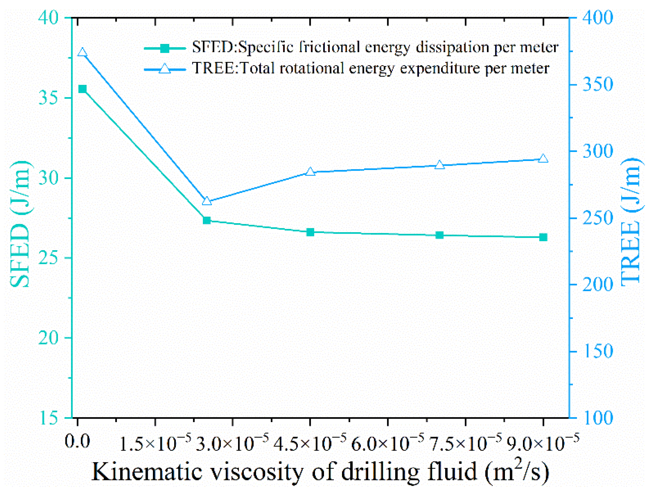
3.2.3. Impact of Kinematic Viscosity

Figure 26 shows the distribution patterns of annular velocity under varying kinematic viscosity. The deviation angle was defined as the angle between the vertical direction and the line connecting the drill string center to the wellbore center, quantifying lateral displacement. As shown in the analysis, variations in kinematic viscosity significantly enhance the coupling effects between drilling fluid and the drill string. At a kinematic viscosity of 1 × 10⁻⁶ m²/s, the drill string deviates to the right by approximately 10.7°. With increasing drilling fluid viscosity, the drill string gradually shifts from rightward to leftward deflection within the borehole, with a critical viscosity threshold of 2.5 × 10⁻⁵ m²/s. At a viscosity of 9 × 10⁻⁵ m²/s, the leftward deflection angle reaches 56.99°. A higher viscosity induces greater internal shear stress in the fluid, enabling the rotating drill string to more effectively drive fluid into the right-side annular clearance. Additionally, increased viscosity significantly amplifies the dynamic pressure effect of the annular fluid, pushing the drill string toward the left borehole wall. Figure 26 further demonstrates that elevated viscosity enlarges radial velocity gradients, with fluid velocities near the wellbore wall notably lower than those adjacent to the drill string. This phenomenon arises because higher viscosity suppresses internal momentum transfer within the fluid, while axial flow cancels out rotational momentum induced by the drill string before it can propagate radially.

Figure 27 shows the trend of annular pressure variation. An increase in kinematic viscosity significantly alters the circumferential pressure distribution: as more fluid is entrained into the right-side clearance channel, the pressure in this region gradually rises to a maximum of approximately 6000 Pa. Conversely, the pressure in the left-side clearance channel decreases substantially, reaching a minimum of about 51 Pa. In heterogeneous shale formations, uneven circumferential pressure distribution can induce localized stress concentration, elevating the risk of wellbore collapse and affecting the transformation of the reservoir. Consequently, the use of high-kinematic-viscosity drilling fluids should be avoided during drilling operations to mitigate these risks.

Furthermore, Figure 28 illustrates the axial velocity distribution in the left annular clearance. At lower kinematic viscosities, the fluid velocity exhibits a relatively uniform axial distribution. However, as the kinematic viscosity increases, the flow regime gradually transitions to laminar flow, with a critical value of 2.5 × 10⁻⁵ m²/s. The narrowing of the clearance due to drill string lateral displacement leads to an expansion of high-velocity fluid zones. The emergence of laminar flow implies that cuttings in the bottom-hole region struggle to be transported upward via circumferential flow. Additionally, the leftward deflection of the drill string further inhibits the removal of bottom-hole cuttings. During shale gas drilling operations, the persistent retention of bottom-hole cuttings can impair fracturing efficiency if not effectively removed, thereby reducing shale gas production rates. Therefore, drilling fluids with a kinematic viscosity higher than 2.5 × 10⁻⁵ m²/s should be used with caution to prevent the occurrence of laminar flow.

Figure 29 shows the effect of kinematic viscosity on friction torque. Compared to direct contact between the drill string and wellbore wall, the presence of drilling fluid effectively reduces friction torque. With the increase in kinematic viscosity, the friction torque continuously decreases, with the maximum reduction reaching 58.31%. This phenomenon occurs because higher kinematic viscosity generates greater dynamic pressure, providing enhanced support and lubrication for the drill string and minimizing direct contact with the wellbore wall.

The variation trends of SFED and TREE shown in Figure 30 indicate that increasing kinematic viscosity effectively reduces frictional energy dissipation. Computational results demonstrate that at a kinematic viscosity of 1 × 10⁻⁶ m²/s, SFED and TREE decrease by 24.28% and 27.41%, respectively. However, when the kinematic viscosity further increases, its improvement on the SFED tends to level off, only showing a slight decrease. Meanwhile, the TREE also gradually increases. The critical value is approximately 2.5 × 10⁻⁵ m²/s, and at this time, the TREE is approximately 262.14 J. This suggests that moderately increasing kinematic viscosity enhances lubrication efficiency, whereas an excessively high viscosity amplifies internal shear stress within the fluid, necessitating additional energy input to sustain drill string motion. It can also be seen from Figure 30 that when an excessively high kinematic viscosity is selected, the frictional contact between the drill string and the wellbore wall will not be significantly improved.

3.2.4. Impact of Density

Figure 31 illustrates the distribution patterns of annular velocity under varying drilling fluid densities. The annular velocity remains largely unchanged with increasing density, indicating that density exerts no significant influence on annular velocity distribution. Conversely, Figure 32 reveals that increased density elevates overall annular pressure, generating localized high-pressure zones (up to 2500 Pa) in the right annular gap, primarily induced by drill string rotation. Furthermore, the radial pressure gradient in the right annular gap intensifies with density, exhibiting lower pressures near the drill string and wellbore walls but peak values in the intermediate zone. This phenomenon is attributed to enhanced centrifugal forces on the drilling fluid under higher densities, which drive excessive fluid accumulation in narrow channels, thereby elevating pressure. While an elevated density prevents cuttings’ deposition and wellbore collapse, the localized high-pressure zones heighten the risk of wellbore leakage. Consequently, intensified annular pressure monitoring is recommended when employing high-density drilling fluids.

Figure 33 details the variation in frictional torque with drilling fluid density and its reduction rate relative to the condition without drilling fluid (approximately 15 N·m, indicated by the dashed gray line). It can be observed that as the drilling fluid density increases from 1000 kg/m³ to 1400 kg/m³, the actual frictional torque significantly decreases from approximately 10.64 N·m to about 8.14 N·m. Although the torque continuously decreases, the marginal benefit of this reduction (i.e., the amount of torque decrease per unit increase in density) slightly decelerates. Correspondingly, the reduction rate of frictional torque, compared to the no-drilling-fluid scenario, substantially increases from about 28% to approximately 45.58%. This significant friction reduction effect is primarily attributed to the superior lubrication and support provided by higher-density drilling fluids: on the one hand, they help form a more stable lubricating film with a higher load-bearing capacity between the drill string and the wellbore wall, effectively isolating metallic contact; on the other hand, an increase in drilling fluid density enhances the buoyant force on the drill string, thereby reducing the normal force exerted by the drill string against the wellbore wall, which directly lowers frictional torque. Additionally, higher-density drilling fluids typically suspend and remove fine abrasive particles more effectively, improving lubrication conditions.

The reduction in frictional torque is directly reflected in the SFED shown in Figure 34, which decreases from approximately 35.56 J/m at 1000 kg/m³ to about 27.0 J/m at 1400 kg/m³, a reduction of about 24.07%. The TREE also decreases with an increasing drilling fluid density, from about 373.57 J/m (at 1000 kg/m³) to approximately 358.9 J/m (at 1400 kg/m³), a reduction of about 3.93%. The reason for TREE’s smaller reduction magnitude compared to that of SFED and frictional torque may be that TREE not only includes the SFED component directly related to wellbore friction but also encompasses energy consumption from internal shearing of the drilling fluid, at the drill bit, or other components, with these additional energy expenditures potentially being less sensitive to changes in drilling fluid density. Collectively, increasing drilling fluid density is an effective technical means for reducing frictional torque and associated energy losses in purely horizontal drilling. However, in practical applications, an excessively high drilling fluid density will significantly increase the circulating pump pressure. Therefore, a balance must be struck, and density should be increased judiciously, possibly in conjunction with appropriate amounts of drag reducers or lubricants, to maximize the potential for friction and energy consumption reduction while effectively controlling the pump pressure.

3.2.5. Comprehensive Parameter Sensitivity Analysis

The influence of fluid parameters on SFED and TREE is summarized in

Table 3. Summary of the influence of fluid parameters on SFED and TREE.

Parameter	Parameter Range	Response Range of Reduction
		SFED	TREE
Flow rate Q (L/min)	30–70	−16.43–32.79%	−21.56–34.6%
Kinematic viscosity η (m2/s)	1 × 10−6–9 × 10−5	−24.28–44.02%	−27.41–49.06%
Density ρ (kg/m3)	1000–1400	−24.28–42.5%	−27.41–30.26%

. Based on the aggregated data, a sensitivity analysis of SFED and TREE was conducted using the range normalization method. To eliminate discrepancies in dimensional units and variation ranges among parameters, a normalized sensitivity index (Equation (25)) was employed to quantify the impact of each parameter on output metrics (SFED and TREE). Furthermore, the relative importance ranking of parameters was calculated via weight Equation (26). A high-sensitivity zone was defined to identify critical thresholds where SFED and TREE exhibited strong responses to fluid parameter variations, with thresholds determined by Equation (27).

$$S_n(p)={\displaystyle \frac{\Delta I(p)}{\Delta p/p_{\mathrm{mid}}}}$$

(25)

where p represents the parameters for analysis (Q, η and ρ), ∆I (p) is the absolute variation in the evaluation index (SFED and TREE) over the parameter range ∆p, and p_mid is the mid-range value.

$$\omega (p)={\displaystyle \frac{S_n(p)}{{\displaystyle {\sum }_{k=1}^N{S}_n(p_k)}}}\times 100\%$$

(26)

where the denominator ∑ represents the sum of all parameter-normalized sensitivity indexes. N represents the total number of parameters. In this study, N = 3.

$$\Gamma ={\mu }_Y+k\cdot {\sigma }_Y$$

(27)

where Y represents the absolute values of the rate of change in the indicators caused by all parameters. μ_Y and σ_Y represent the arithmetic mean and standard deviation of the absolute values of the rate of change in SFED or TREE, respectively. k represents the engineering safety factor. In this study, k is set to 1.3.

The final sensitivity analysis results are illustrated in Figure 35. The SFED and TREE values under no-drilling-fluid conditions were used as baseline references, while reductions in SFED and TREE due to drilling fluid parameters are represented as negative values. As shown in the figure, a higher viscosity (9 × 10⁻⁵ m²/s) resulted in a maximum reduction of 44.0% for SFED, whereas at a lower viscosity (2.5 × 10⁻⁵ m²/s), the TREE reduction reached 49.1%. Additionally, when the density was set at 1400 kg/m³, the SFED reduction exceeded 40%, reaching 42.5%, indicating that higher viscosities and densities significantly reduce both SFED and TREE. On the other hand, sensitivity analysis revealed that SFED is most sensitive to variations in density; thus, controlling density is crucial for reducing SFED. Conversely, TREE exhibits the highest sensitivity to flow rate changes, making flow rate control essential for minimizing TREE. However, viscosities exceeding 2.5 × 10⁻⁵ led to an increase in TREE, suggesting that viscosity should be maintained below this threshold.

The high-sensitivity region thresholds for SFED and TREE were 20.05% and 23.92%, respectively. These values indicate that within typical drilling fluid parameter ranges, both SFED and TREE exhibit pronounced responses to parameter variations.

3.3. Impact of Formation and Friction

In shale gas exploitation, variations in formation depth and reservoir properties result in a wide range of Young’s modulus values for wellbore walls. The dynamic response of the drill string to different formations directly impacts wellbore stability and drilling parameter selection. Figure 36 illustrates the contact force in formations with varying Young’s modulus. The collision contact force exhibits a pronounced periodic variation trend, with both its amplitude and frequency increasing as Young’s modulus increases. A higher Young’s modulus indicates higher formation hardness; during drill string–wellbore collisions, elevated contact stiffness leads to larger normal contact forces, stronger rebound effects, and intensified perturbations on the wellbore wall. In softer formations, the drill string will not experience excessive rebound. However, the damping effect of softer formations can also have a hysteresis effect on the movement of the drill string, which is not conducive to the elastic recovery of the deformed drill string to a certain extent.

As illustrated in Figure 37, the kinetic energy of the drill string increases sharply with the elevation of the formation Young’s modulus, reaching a maximum of 1384.69 J. This phenomenon primarily arises because, in harder formations, the drill string undergoes significant rebound due to contact impact forces, whereas in softer formations, a substantial portion of the energy is absorbed by the formations, thereby suppressing random vibrations. Consequently, when drilling through hard formations, particular attention should be paid to mitigating drill string vibrations to prevent wellbore instability and drill string failure.

Figure 38 illustrates the influence of the friction coefficient between the drill string and the wellbore wall on annular velocity distribution. The friction coefficient primarily affects annular velocity by altering the drill string’s dynamic behavior. When the friction coefficient is 0.07, the drill string deflects leftward by 5.66° due to the dynamic pressure effect of the fluid in the right clearance. However, the fluid velocity in the right clearance remains higher than that in the left clearance, influenced by the drill string’s rotation direction. At a friction coefficient of 0.15, the leftward deviation angle reduces to 0.58°. As the friction coefficient increases further, the drill string gradually shifts rightward, reaching a maximum deviation angle of 20.83° at a friction coefficient of 0.5.

Although the drill string exhibits leftward deviation under low friction coefficients, the rotational motion of the drill string induces a tendency to climb upward along the right side of the wellbore. Consequently, the leftward deviation angle remains small, reducing the probability of asymmetric cuttings’ accumulation in the annulus. As previously analyzed, drilling fluid viscosity significantly influences the deviation angle of the drill string. To mitigate excessive lateral displacement, adjusting the drilling fluid viscosity can help keep the drill string in the optimal position. Specifically, when the formation exhibits low friction coefficients, reducing the kinematic viscosity of the drilling fluid can minimize leftward deviation. Conversely, in formations with high friction coefficients, the addition of drag reducers and increased kinematic viscosity can effectively improve the deviation of the drill string.

To enhance field performance based on FSI insights, the following adaptive strategies may be considered: (1) During pump pressure escalation (0.5–8 MPa), prioritize real-time monitoring of low-order vibration modes to enable prompt mitigation measures against resonance. (2) Optimize hydraulics by keeping viscosity within 1–2.5 × 10⁻⁵ m²/s and elevating the flow rate to 55–60 L/min, reducing SFED and TREE while preventing laminar flow. (3) For formations with a friction coefficient < 0.15, reducing viscosity may suppress leftward deflection; with a friction coefficient > 0.15, implement dual measures: injecting drag reducers AND moderately increasing viscosity (1–2.5 × 10⁻⁵ m²/s) to promote drill string centralization. (4) In high-modulus zones (>20 GPa), deploy distributed dampers at ~30 m intervals, modestly increase flow rate to 60 L/min, implement stepwise RPM elevation, and judiciously elevate viscosity (≤2.5 × 10⁻⁵ m²/s)—collectively attenuating impact forces while keeping the equivalent circulating density (ECD) within safe limits via real-time diagnostics.

4. Conclusions

Excessive friction, fluid–structure interaction vibrations, and energy consumption in deep shale gas horizontal wells severely restrict their efficient and sustainable development. To address these challenges, this study developed and experimentally validated a bidirectional FSI model for a 76 mm slim-hole drill string–drilling fluid system. Compared to explicit dynamic analysis, the recursive algorithm developed herein reduces the computation time by 59.3% while maintaining an equivalent accuracy. The key findings are summarized as follows:

(1)

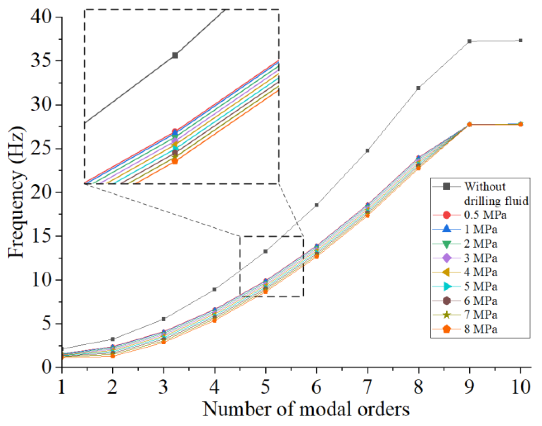
Drilling fluid lowers the drill string natural frequency by 20–25%, with low-order modes showing lateral coupled vibrations. An increased pump pressure (0.5–8 MPa) further reduces the second-order frequency by up to 46.5%, requiring monitoring of the low-order modes to prevent resonance.

(2)

Dominant frictional energy dissipation occurs from persistent drill string–wellbore contact (lower right). Eccentric annular fluid pressure significantly reduces this friction; under benchmark conditions, SFED and TREE decreased by 24.28% and 27.41%, respectively. While most parameter increases reduce SFED, TREE slightly rises if viscosity exceeds 2.5 × 10⁻⁵ m²/s, leading to laminar flow detrimental to wellbore cleaning.

(3)

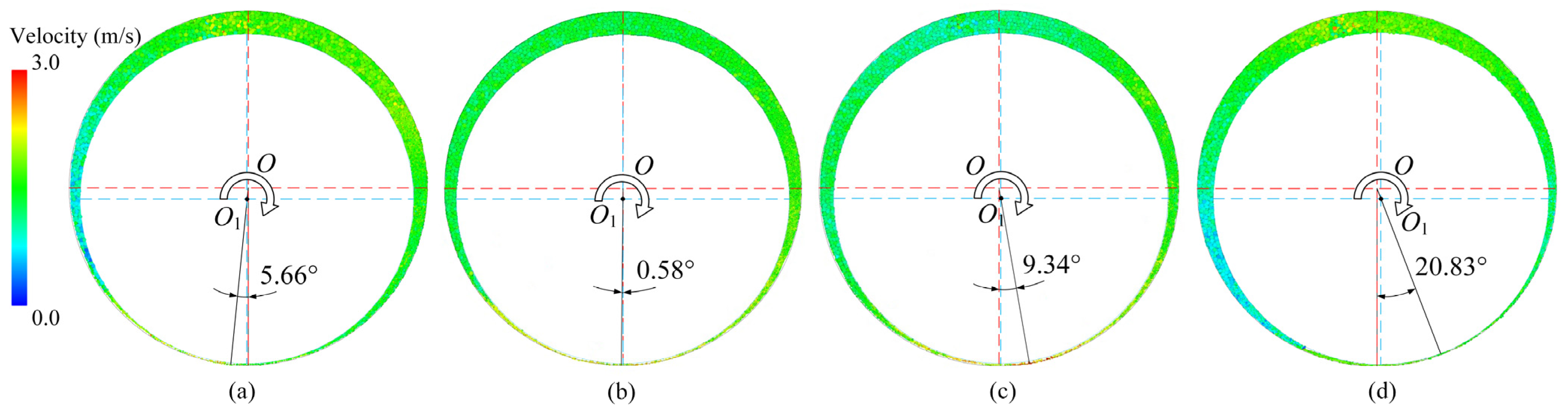
Horizontal drill string displacement favors the right side, but a kinematic viscosity > 2.5 × 10⁻⁵ m²/s causes anomalous leftward shifts and introduces radial velocity gradients. Inherent circumferential flow asymmetry aids wellbore cleaning.

(4)

A critical friction coefficient of 0.15 stabilizes the drill string centrally. Excessive lateral displacement causes asymmetric cuttings’ accumulation, impacting fracturing. Managing viscosity and drag reducers based on subcritical or supercritical friction is key to controlling deflection and cuttings buildup.

(5)

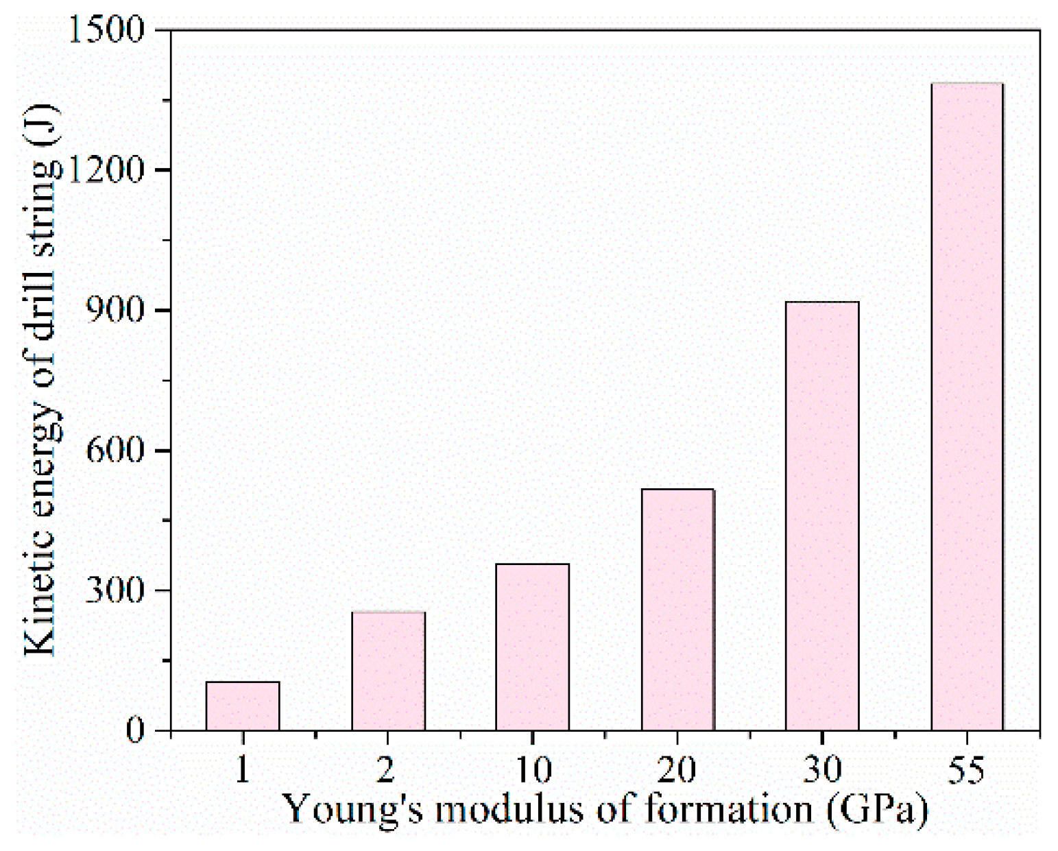
High-Young’s-modulus formations increase drill string vibrations, the lateral coupled resonance risk, impact forces, and failure likelihood.

Despite its computational efficiency, the recursive algorithm’s robustness and convergence under challenging conditions (e.g., extreme deformations, complex contacts) require further evaluation. The current FSI framework, while foundational for friction–vibration–energy coupling, neglects shale anisotropy, gas influx, and cuttings interactions. Future work will enhance predictive capabilities by (a) integrating shale heterogeneity effects using well log data and (b) coupling advanced viscosity and cuttings’ transport models. Nevertheless, the model’s validated thresholds (e.g., viscosity 1–2.5 × 10⁻⁵ m²/s, critical friction 0.15) remain directly applicable to 76 mm slim-hole designs.

References

1. Sabanov, S.; Qureshi, A.R.; Dauitbay, Z.; Kurmangazy, G. A Method for the Modified Estimation of Oil Shale Mineable Reserves for Shale Oil Projects: A Case Study. Energies 2023, 16, 5853. [Google Scholar] [CrossRef]
2. Jintao, A.; Jun, L.; Huang, H.; Zhang, H.; Yang, H.; Zhang, G.; Chen, S.; Lai, Q. Analysis of Cuttings Transport in Small-Bore Horizontal Wells Considering Drill String Eccentricity. Energy Sci. Eng. 2025, 13, 3088–3106. [Google Scholar] [CrossRef]
3. Tengesdal, N.K.; Fotland, G.; Holden, C.; Haugen, B. Modeling of drill string dynamics in directional wells for real-time simulation. Simulation 2023, 99, 937–956. [Google Scholar] [CrossRef]
4. Nguyen, K.-L.; Tran, Q.-T.; Andrianoely, M.-A.; Manin, L.; Baguet, S.; Dufour, R.; Mahjoub, M.; Menand, S. Nonlinear rotordynamics of a drillstring in curved wells: Models and numerical techniques. Int. J. Mech. Sci. 2020, 166, 105225. [Google Scholar] [CrossRef]
5. Liu, Y.; Niu, Y.; Guan, Z.; Lyu, S. The review and development of devices with an increasing rate of penetration (ROP) in deep formation drilling based on drill string vibration. Energies 2022, 15, 7377. [Google Scholar] [CrossRef]
6. Berlioz, A.; Der Hagopian, J.; Dufour, R.; Draoui, E. Dynamic Behavior of a Drill-String: Experimental Investigation of Lateral Instabilities. J. Vib. Acoust. 1996, 118, 292–298. [Google Scholar] [CrossRef]
7. Tchomeni Kouejou, B.X.; Sozinando, D.F.; Anyika Alugongo, A. Modeling and Analysis of Drill String–Casing Collision under the Influence of Inviscid Fluid Forces. Appl. Sci. 2023, 13, 3557. [Google Scholar] [CrossRef]
8. Mohammadzadeh, M.; Arbabtafti, M.; Shahgholi, M.; Yang, J. Nonlinear vibrations of composite drill strings considering drill string–wellbore contact and bit–rock interaction. Arch. Appl. Mech. 2022, 92, 2569–2592. [Google Scholar] [CrossRef]
9. Patil, P.A.; Teodoriu, C. A comparative review of modelling and controlling torsional vibrations and experimentation using laboratory setups. J. Pet. Sci. Eng. 2013, 112, 227–238. [Google Scholar] [CrossRef]
10. Goicoechea, H.E.; Lima, R.; Sampaio, R. How to mathematically model a drill-string: Lumped or continuous models? Chaos Solitons Fractals 2024, 188, 115543. [Google Scholar] [CrossRef]
11. Bembenek, M.; Grydzhuk, Y.; Gajdzik, B.; Ropyak, L.; Pashechko, M.; Slabyi, O.; Al-Tanakchi, A.; Pryhorovska, T. An analytical–numerical model for determining “drill string–wellbore” frictional interaction forces. Energies 2024, 17, 301. [Google Scholar] [CrossRef]
12. Heisig, G.; Neubert, M. Lateral Drillstring Vibrations in Extended-Reach Wells. In Proceedings of the IADC/SPE Drilling Conference, New Orleans, LA, USA, 23 February 2000. [Google Scholar]
13. Galasso, S.; Santelli, L.; Zambetti, R.; Giusteri, G.G. Simulation of drill-string systems with fluid–structure and contact interactions in realistic geometries. Comput. Mech. 2024, 75, 1165–1189. [Google Scholar] [CrossRef]
14. Chodankar, A.D.; Seibi, A. Effects of axial compression load, borehole clearance, and contact force using axial-lateral fluid coupled drill string vibration model. In Proceedings of the ASME International Mechanical Engineering Congress and Exposition, Salt Lake City, UT, USA, 11–14 November 2019; American Society of Mechanical Engineers: New York, NY, USA, 2019; p. V004T05A112. [Google Scholar]
15. Tengesdal, N.K.; Holden, C.; Pedersen, E. Component-based modeling and simulation of nonlinear drill-string dynamics. J. Offshore Mech. Arct. Eng. 2022, 144, 021801. [Google Scholar] [CrossRef]
16. Neto, H.J.C.; Trindade, M.A. Mitigation of negative damping effects in deep drilling operations through active control. J. Sound Vib. 2025, 610, 119078. [Google Scholar] [CrossRef]
17. Barjini, A.H.; Khoshnazar, M.; Moradi, H. Design of a sliding mode controller for suppressing coupled axial & torsional vibrations in horizontal drill strings using Extended Kalman Filter. J. Sound Vib. 2024, 586, 118477. [Google Scholar]
18. Ejike, C.; Abid, K.; Teodoriu, C. Scaling Torsional Drilling Vibrations: A Simulation-Based Comparison of Downscale and Upscale Drill Strings Under Varying Torque Conditions. Appl. Sci. 2025, 15, 2399. [Google Scholar] [CrossRef]
19. Arjun Patil, P.; Teodoriu, C. Model development of torsional drillstring and investigating parametrically the stick-slips influencing factors. J. Energy Resour. Technol. 2013, 135, 013103. [Google Scholar] [CrossRef]
20. Chen, W.; Cao, Y.; Guo, X.; Ma, H.; Wen, B.; Wang, B. Semi-analytical dynamic modeling and fluid-structure interaction analysis of L-shaped pipeline. Thin-Walled Struct. 2024, 196, 111485. [Google Scholar] [CrossRef]
21. Bouaanani, N.; Miquel, B. Efficient modal dynamic analysis of flexible beam–fluid systems. Appl. Math. Model. 2015, 39, 99–116. [Google Scholar] [CrossRef]
22. Abdollahi, R.; Firouz-abadi, R.D.; Rahmanian, M. On the stability of rotating pipes conveying fluid in annular liquid medium. J. Sound Vib. 2021, 494, 115891. [Google Scholar] [CrossRef]
23. Liao, M.; Zhou, Y.; Su, Y.; Lian, Z.; Jiang, H. Dynamic analysis and multi-objective optimization of an offshore drilling tube system with pipe-in-pipe structure. Appl. Ocean. Res. 2018, 75, 85–99. [Google Scholar] [CrossRef]
24. Matuck, G.A.; Gama, A.L.; Lannes, D.P.; Bento, T.F.B. Hydrodynamic mass and damping of horizontal tubes subjected to internal two-phase flow. J. Sound Vib. 2022, 532, 117004. [Google Scholar] [CrossRef]
25. Pei, Y.-C.; Sun, Y.-H.; Wang, J.-X. Dynamics of rotating conveying mud drill string subjected to torque and longitudinal thrust. Meccanica 2013, 48, 2189–2201. [Google Scholar] [CrossRef]
26. Fujita, K.; Moriasa, A. Stability of cantilevered pipes subjected to internal flow and external annular axial flow simultaneously. In Proceedings of the Pressure Vessels and Piping Conference, Boston, MA, USA, 19–23 July 2015; American Society of Mechanical Engineers: New York, NY, USA, 2015; p. V004T04A020. [Google Scholar]
27. Paı, M.; Luu, T.; Prabhakar, S. Dynamics of a long tubular cantilever conveying fluid downwards, which then flows upwards around the cantilever as a confined annular flow. J. Fluids Struct. 2008, 24, 111–128. [Google Scholar]
28. Mihajlović, N.; van Veggel, A.A.; van de Wouw, N.; Nijmeijer, H. Analysis of Friction-Induced Limit Cycling in an Experimental Drill-String System. J. Dyn. Syst. Meas. Control. 2005, 126, 709–720. [Google Scholar] [CrossRef]
29. Tran, Q.-T.; Nguyen, K.-L.; Manin, L.; Andrianoely, M.-A.; Dufour, R.; Mahjoub, M.; Menand, S. Nonlinear dynamics of directional drilling with fluid and borehole interactions. J. Sound Vib. 2019, 462, 114924. [Google Scholar] [CrossRef]
30. Ozbayoglu, E.M.; Erge, O.; Ozbayoglu, M.A. Predicting the pressure losses while the drillstring is buckled and rotating using artificial intelligence methods. J. Nat. Gas Sci. Eng. 2018, 56, 72–80. [Google Scholar] [CrossRef]
31. Abdo, J.; Al-Shabibi, A.; Al-Sharji, H. Effects of tribological properties of water-based drilling fluids on buckling and lock-up length of coiled tubing in drilling operations. Tribol. Int. 2015, 82, 493–503. [Google Scholar] [CrossRef]
32. Abdo, J.; Haneef, M. Clay nanoparticles modified drilling fluids for drilling of deep hydrocarbon wells. Appl. Clay Sci. 2013, 86, 76–82. [Google Scholar] [CrossRef]
33. Liyanarachchi, S.; Rideout, G. Improved stiff string torque and drag prediction using a computationally efficient contact algorithm. Math. Comput. Model. Dyn. Syst. 2024, 30, 417–443. [Google Scholar] [CrossRef]
34. Moharrami, M.J.; de Arruda Martins, C.; Shiri, H. Nonlinear integrated dynamic analysis of drill strings under stick-slip vibration. Appl. Ocean. Res. 2021, 108, 102521. [Google Scholar] [CrossRef]
35. Guo, X.; Qiu, Z.; Li, M.; Li, X.; Hu, N.; Zhao, L.; Ye, C. Axial-torsional coupling vibration model and nonlinear behavior of drill string system in oil and gas wells. Commun. Nonlinear Sci. Numer. Simul. 2025, 142, 108560. [Google Scholar] [CrossRef]
36. Asghar Jafari, A.; Kazemi, R.; Faraji Mahyari, M. The effects of drilling mud and weight bit on stability and vibration of a drill string. J. Vib. Acoust. 2012, 134, 011014. [Google Scholar] [CrossRef]
37. Tang, S.; Liang, Z.; Zhao, G.-H. Stability of transverse vibration of drillstring conveying drilling fluid. J. Theor. Appl. Mech. 2020, 58, 1061–1074. [Google Scholar] [CrossRef]
38. Guzek, A.; Shufrin, I.; Pasternak, E.; Dyskin, A.V. Influence of drilling mud rheology on the reduction of vertical vibrations in deep rotary drilling. J. Pet. Sci. Eng. 2015, 135, 375–383. [Google Scholar] [CrossRef]
39. Passos Volpi, L.; Cayeux, E.; Wiggo Time, R. A Coupled Fluid-Structure Model for Estimation of Hydraulic Forces on the Drill-Pipes. J. Offshore Mech. Arct. Eng. 2024, 146, 031801. [Google Scholar] [CrossRef]
40. Al Dushaishi, M.F.; Nygaard, R.; Stutts, D.S. Effect of drilling fluid hydraulics on drill stem vibrations. J. Nat. Gas Sci. Eng. 2016, 35, 1059–1069. [Google Scholar] [CrossRef]
41. Liu, J.; Chen, Y.; Liang, S.; Cai, M.; Md, Y. Influence of non-Newton rheological parameters of drilling fluid on axial-lateral-torsional coupling vibration of rotating drill string. Geoenergy Sci. Eng. 2024, 232, 212415. [Google Scholar] [CrossRef]
42. Volpi, L.; Cayeux, E.; Time, R.W. Whirling dynamics of a drill-string with fluid–structure interaction. Geoenergy Sci. Eng. 2024, 232, 212423. [Google Scholar] [CrossRef]
43. Luo, Y.; Qian, F.; Sun, H.; Wang, X.; Chen, A.; Zuo, L. Rigid-flexible coupling multi-body dynamics modeling of a semi-submersible floating offshore wind turbine. Ocean. Eng. 2023, 281, 114648. [Google Scholar] [CrossRef]
44. Samei, H.; Chhabra, R. SuRFR: A fast recursive simulator for soft manipulators with discrete joints on SE (3). Mech. Mach. Theory 2024, 194, 105589. [Google Scholar] [CrossRef]
45. Schiehlen, W.; Guse, N.; Seifried, R. Multibody dynamics in computational mechanics and engineering applications. Comput. Methods Appl. Mech. Eng. 2006, 195, 5509–5522. [Google Scholar] [CrossRef]
46. Liu, C.; Tian, Q.; Hu, H. Dynamics and control of a spatial rigid-flexible multibody system with multiple cylindrical clearance joints. Mech. Mach. Theory 2012, 52, 106–129. [Google Scholar] [CrossRef]
47. Tian, Q.; Lou, J.; Mikkola, A. A new elastohydrodynamic lubricated spherical joint model for rigid-flexible multibody dynamics. Mech. Mach. Theory 2017, 107, 210–228. [Google Scholar] [CrossRef]
48. Zheng, E.; Wang, T.; Guo, J.; Zhu, Y.; Lin, X.; Wang, Y.; Kang, M. Dynamic modeling and error analysis of planar flexible multilink mechanism with clearance and spindle-bearing structure. Mech. Mach. Theory 2019, 131, 234–260. [Google Scholar] [CrossRef]
49. Li, X.; Shao, W.; Tang, J.; Zhang, D.; Chen, J.; Zhao, J.; Wen, Y. Multi-physics field coupling interface lubrication contact analysis for gear transmission under various finishing processes. Eng. Fail. Anal. 2024, 165, 108742. [Google Scholar] [CrossRef]
50. Gonzalez-Perez, I.; Iserte, J.L.; Fuentes, A. Implementation of Hertz theory and validation of a finite element model for stress analysis of gear drives with localized bearing contact. Mech. Mach. Theory 2011, 46, 765–783. [Google Scholar] [CrossRef]
51. Zhou, C.; Wang, H. An adhesive wear prediction method for double helical gears based on enhanced coordinate transformation and generalized sliding distance model. Mech. Mach. Theory 2018, 128, 58–83. [Google Scholar] [CrossRef]
52. Zhang, Y.; Xu, L. Curvature-based framework for contact analysis of complex tooth surfaces. Int. J. Mech. Sci. 2025, 293, 110147. [Google Scholar] [CrossRef]
53. Chen, S.; Wei, J.; Wei, H.; Tan, Y.; Liu, C. A comprehensive mesh stiffness model for heavy-duty spiral bevel gear pair based on design and manufacturing collaboration. Mech. Mach. Theory 2025, 209, 106005. [Google Scholar] [CrossRef]
54. Bu, H.; Li, J.; Guo, J.; Gao, Z.; Zhao, Y. Establishment of theoretical model and dynamic analysis of gear meshing force for the multi-gear driving system considering the effect of friction. Eng. Fail. Anal. 2025, 171, 109382. [Google Scholar] [CrossRef]
55. Chen, H.; Zhang, K.; Piao, M.; Wang, X.; Mao, J.; Song, Q. Virtual Simulation Analysis of Rigid-Flexible Coupling Dynamics of Shearer with Clearance. Shock. Vib. 2018, 2018, 6179054. [Google Scholar] [CrossRef]
56. Deng, X.; Wang, S.; Hammi, Y.; Qian, L.; Liu, Y. A combined experimental and computational study of lubrication mechanism of high precision reducer adopting a worm gear drive with complicated space surface contact. Tribol. Int. 2020, 146, 106261. [Google Scholar] [CrossRef]
57. Renzi, E.; Dias, F. Application of a moving particle semi-implicit numerical wave flume (MPS-NWF) to model design waves. Coast. Eng. 2022, 172, 104066. [Google Scholar] [CrossRef]
58. Khayyer, A.; Tsuruta, N.; Shimizu, Y.; Gotoh, H. Multi-resolution MPS for incompressible fluid-elastic structure interactions in ocean engineering. Appl. Ocean. Res. 2019, 82, 397–414. [Google Scholar] [CrossRef]
59. Liu, X.; Morita, K.; Zhang, S. An advanced moving particle semi-implicit method for accurate and stable simulation of incompressible flows. Comput. Methods Appl. Mech. Eng. 2018, 339, 467–487. [Google Scholar] [CrossRef]
60. Bazaluk, O.; Velychkovych, A.; Ropyak, L.; Pashechko, M.; Pryhorovska, T.; Lozynskyi, V. Influence of heavy weight drill pipe material and drill bit manufacturing errors on stress state of steel blades. Energies 2021, 14, 4198. [Google Scholar] [CrossRef]
61. Chudyk, I.; Sudakova, D.; Dreus, A.; Pavlychenko, A.; Sudakov, A. Determination of the thermal state of a block gravel filter during its transportation along the borehole. Min. Miner. Depos. 2023, 17, 75–82. [Google Scholar] [CrossRef]
Figure 1. Contact relationship between drill pipe and wellbore wall: (a) internal contact relationship; (b) equivalent representation of the contact between the drill string and wellbore wall.
Applsci 15 06743 g001
Figure 2. Geometric relationship of the contact area.
Applsci 15 06743 g002
Figure 3. Effective computational radius of fluid particles.
Applsci 15 06743 g003
Figure 4. Relationship between particle size and total pressure.
Applsci 15 06743 g004
Figure 5. Drill string and wellbore wall models.
Applsci 15 06743 g005
Figure 6. Schematic diagram of the drill string–drilling fluid coupled model.
Applsci 15 06743 g006
Figure 7. Flow chart of fluid–structure interaction analysis.
Applsci 15 06743 g007
Figure 8. Indoor simulated drilling experimental platform: (a) overall view of the experimental platform; (b) schematic diagram of the sensor connection; (c) data acquisition system; (d) software.
Applsci 15 06743 g008
Figure 9. Variation trend of driving torque with feed pressure.
Applsci 15 06743 g009
Figure 10. Variation trend of annular outlet velocity with flow rate of drilling fluid in the wellbore.
Applsci 15 06743 g010
Figure 11. Trajectory of the drill string center at different rotational speeds: (a) 3.67 L/min, 256 rpm; (b) 3.67 L/min, 435 rpm.
Applsci 15 06743 g011
Figure 12. Selection rules for tracer particles in drill string internal fluid.
Applsci 15 06743 g012
Figure 13. Particle motion paths under different drilling parameters: (a) 30 L/min, 600 rpm; (b) 50 L/min, 400 rpm; (c) 50 L/min, 600 rpm.
Applsci 15 06743 g013
Figure 14. Effect of rotational speeds on drill string dynamics considering drill string internal fluid interaction.
Applsci 15 06743 g014
Figure 15. Effect of feed pressure on drill string dynamics considering drill string internal fluid interaction.
Applsci 15 06743 g015
Figure 16. Effect of rotational speeds on drill string dynamics considering annular fluid interaction.
Applsci 15 06743 g016
Figure 17. Effect of feed pressure on drill string dynamics considering annular fluid interaction.
Applsci 15 06743 g017
Figure 18. Annular velocity field under different rotational speeds: (a) 400 rpm; (b) 600 rpm; (c) 800 rpm.
Applsci 15 06743 g018
Figure 19. Annular velocity field under different feed pressures: (a) 10 kN; (b) 13 kN; (c) 15 kN.
Applsci 15 06743 g019
Figure 20. Boundary conditions of the drill string: (a) constraint; (b) spring support.
Applsci 15 06743 g020
Figure 21. Drill string modal frequencies under drilling fluid conditions.
Applsci 15 06743 g021
Figure 22. Effect of pump pressure on drill string vibration frequencies.
Applsci 15 06743 g022
Figure 23. The effect of flow rate of drilling fluid on friction torque.
Applsci 15 06743 g023
Figure 24. SFED and TREE versus drilling fluid flow rate.
Applsci 15 06743 g024
Figure 25. Distribution patterns of annular velocity under varying drilling fluid flow rates: (a) 30 L/min; (b) 50 L/min; (c) 70 L/min.
Applsci 15 06743 g025
Figure 26. Distribution patterns of annular velocity under varying kinematic viscosity: (a) 1 × 10⁻⁶ m2/s; (b) 2.5 × 10⁻⁵ m2/s; (c) 4.5 × 10⁻⁵ m2/s; (d) 9 × 10⁻⁵ m2/s.
Applsci 15 06743 g026
Figure 27. Distribution patterns of annular pressure under varying kinematic viscosity: (a) 1 × 10⁻⁶ m2/s; (b) 2.5 × 10⁻⁵ m2/s; (c) 4.5 × 10⁻⁵ m2/s; (d) 9 × 10⁻⁵ m2/s.
Applsci 15 06743 g027
Figure 28. Axial velocity under different kinematic viscosities: (a) 1 × 10⁻⁶ m2/s; (b) 2.5 × 10⁻⁵ m2/s; (c) 4.5 × 10⁻⁵ m2/s; (d) 9 × 10⁻⁵ m2/s.
Applsci 15 06743 g028
Figure 29. The effect of kinematic viscosity of drilling fluid on friction torque.
Applsci 15 06743 g029
Figure 30. SFED and TREE versus kinematic viscosity of drilling fluid.
Applsci 15 06743 g030
Figure 31. Distribution patterns of annular velocity under varying density of drilling fluid: (a) 1000 kg/m3; (b) 1200 kg/m3; (c) 1400 kg/m3.
Applsci 15 06743 g031
Figure 32. Distribution patterns of annular pressure under varying density of drilling fluid: (a) 1000 kg/m3; (b) 1200 kg/m3; (c) 1400 kg/m3.
Applsci 15 06743 g032
Figure 33. The effect of density of drilling fluid on friction torque.
Applsci 15 06743 g033
Figure 34. SFED and TREE versus density of drilling fluid.
Applsci 15 06743 g034
Figure 35. Sensitivity analyses of SFED and TREE.
Applsci 15 06743 g035
Figure 36. Contact force in formations with varying Young’s modulus.
Applsci 15 06743 g036
Figure 37. Kinetic energy of drill string in formations with varying Young’s modulus.
Applsci 15 06743 g037
Figure 38. Distribution patterns of annular velocity under varying friction coefficients: (a) μ = 0.07; (b) μ = 0.15; (c) μ = 0.3; (d) μ = 0.5.
Applsci 15 06743 g038