Complex-Valued CNN-Based Defect Reconstruction of Carbon Steel from Eddy Current Signals

Abstract

Eddy current testing (ECT) has become a widely adopted technique for non-destructive testing (NDT) due to its effectiveness in detecting surface and near-surface defects in conductive materials. However, traditional methods mainly focus on defect detection and face significant challenges in extracting geometric information such as defect size and shape, which is crucial for structural health monitoring (SHM) and remaining useful life (RUL) assessment. To address these challenges, this study proposes a defect reconstruction approach based on a complex-valued convolutional neural network (CV-CNN), which directly leverages both amplitude and phase information inherent in complex-valued impedance signals. The proposed framework employs convolution, pooling, and activation operations specifically designed within the complex-valued domain to facilitate the high-fidelity reconstruction of defect morphology as well as precise multi-class defect classification. Notably, this approach processes the complete complex-valued signal without relying on prior structural parameters or baseline data, thereby achieving substantial improvements in both defect visualization and classification performance. Moreover, when compared to a complex-valued fully convolutional neural network (CV-FCNN), CV-CNN demonstrates a superior average classification accuracy of 85%, significantly outperforming the CV-FCNN model. Experimental results on carbon steel specimens with standard electrical discharge machining (EDM) notches under multi-frequency excitation confirm these advantages. This contribution provides a promising solution in the field of NDT for intelligent and precise defect detection.

1. Introduction

Non-destructive testing (NDT) is a class of techniques that is used to find internal or surface defects without destroying the integrity of the material or structure. Among the many NDT methods, eddy current testing (ECT) is widely used in aerospace, petrochemical, and other fields for component and pipe inspection due to its sensitivity to surface and near-surface defects in conductive materials [1]. Although traditional ECT techniques can effectively identify the presence of defects, there are obvious deficiencies in the extraction of defect geometrical information (e.g., size and shape), which is crucial for structural health monitoring (SHM) and remaining useful life (RUL) assessment.

To overcome these limitations, researchers have gradually introduced deep learning methods, especially neural networks, to model and resolve the deep features in eddy current signals. In earlier studies, Wrzuszczak et al. [2] used neural networks to achieve the feature classification of multi-frequency eddy current signals, while Zhou et al. [3] accurately predicted the length and depth of cracks by back-propagation neural networks. To address the problem of blurred ECT images, Rao et al. [4] combined image processing and neural network methods to achieve the high-fidelity recovery of the defect geometry. In addition, multi-task learning combined with deep neural networks has also been used to enhance detection robustness and classification efficiency [5] and the Lissajous graphical classification method proposed by D’Angelo et al. [6], and it significantly improves the efficiency of fast defect classification in ECT. The detection capability of ECT in various fields such as aerospace, pipelines, and thin film materials has also been significantly enhanced by the application of deep learning [7,8,9]. In recent years, there has been a rise in pictorial eddy current signal analysis methods, such as eddy current thermography and C-scanning, which help to visualize defect morphology more intuitively, and this type of representation in the form of images facilitates the application of deep learning methods in defect recognition [10].

Based on this, deep learning methods, especially convolutional neural networks (CNNs), have demonstrated strong capabilities in defect detection, classification and reconstruction. CNNs can automatically extract multi-scale spatial and temporal features implicit in ECT signals, breaking through the limitations of traditional signal processing methods in feature design and non-linear modeling. For example, the multi-scale spatio-temporal self-attention (MSTSA) network introduces spatial and temporal attention mechanisms into ECT signal processing, which significantly improves the accuracy and efficiency of defect recognition [11]. In addition, several studies have used neural networks for effective reconstruction and regression prediction of defect morphology, including inverse methods and finite element simulations to extract defect geometric features [12,13,14]. Multi-channel data fusion, image processing and feature learning have also been used for three-dimensional (3D) defect reconstruction and multi-scale defect recognition [15,16,17]. Meanwhile, neural networks have also been used in defect classification and multiparameter estimation tasks [18,19,20,21,22].

However, traditional CNNs mainly deal with real-domain signals and cannot fully utilize the magnitude and phase information in ECT signals, thus limiting their capability in high-resolution defect reconstruction. Some studies have begun to try to improve the reconstruction performance by using complex-valued modeling, such as mapping ECT signals into images and then performing convolutional processing, but still do not fully utilize the structural information in the complex-valued signals themselves [20,22]. In contrast, complex-valued CNN (CV-CNN) has the natural ability to process complex-valued signals and can simultaneously learn the coupling relationship between amplitude and phase, which provides a new method for high-precision defect reconstruction [23,24,25,26].

Based on the above background, this study proposes a defect reconstruction method based on CV-CNN for ECT signal enhancement and the classification and identification of carbon steel materials. By acquiring the eddy current signals of carbon steel standard defects at different frequencies, the high-precision extraction and reconstruction of defect features are achieved. The experimental results show that the method has excellent classification performance and strong generalization ability in multi-category defect recognition. The main contributions of this paper are summarized as follows:

• A 2D defect reconstruction method based on complex-valued eddy current signals is proposed, which effectively enhances defect visualization and sharpens defect boundaries.
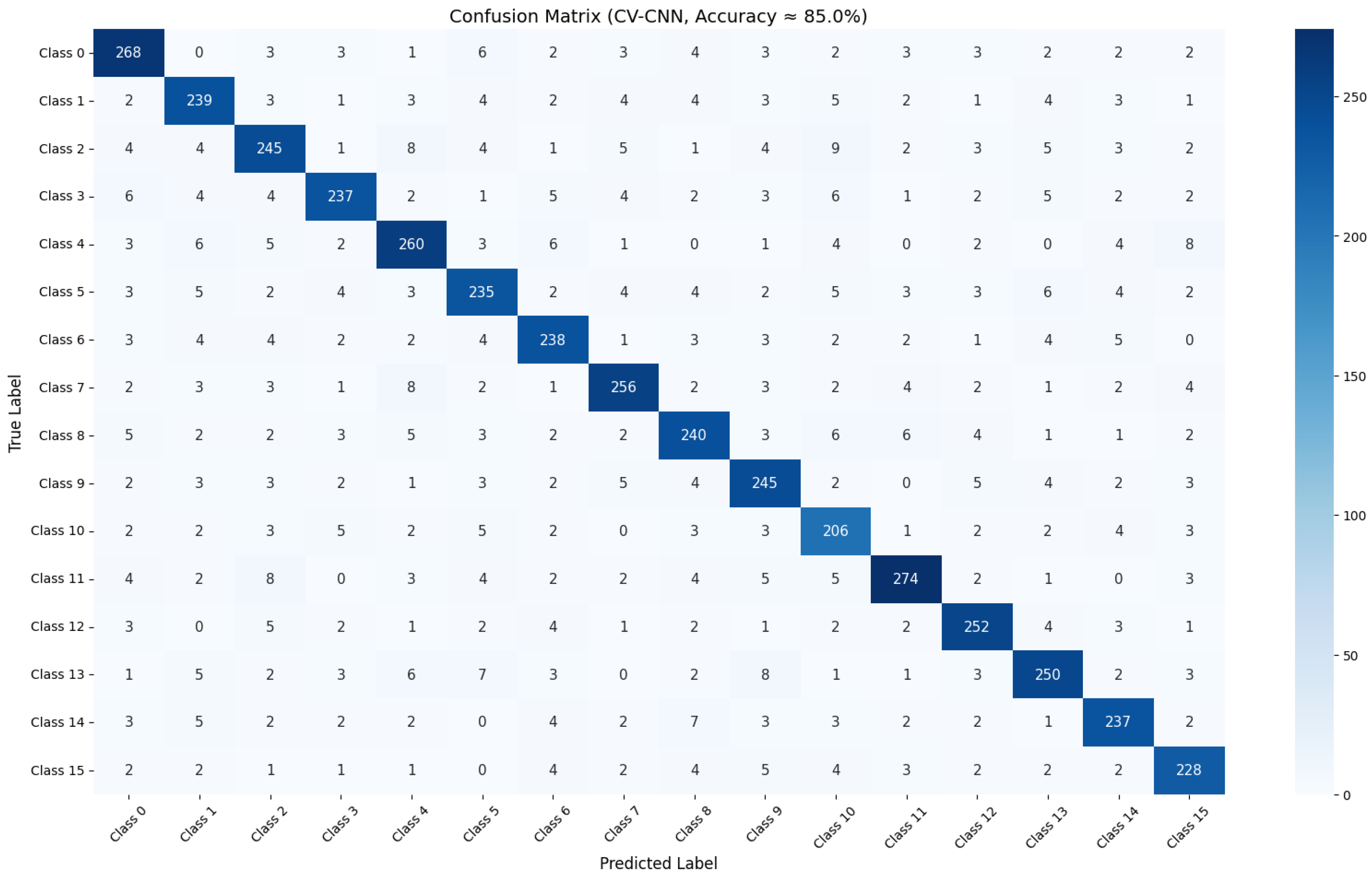
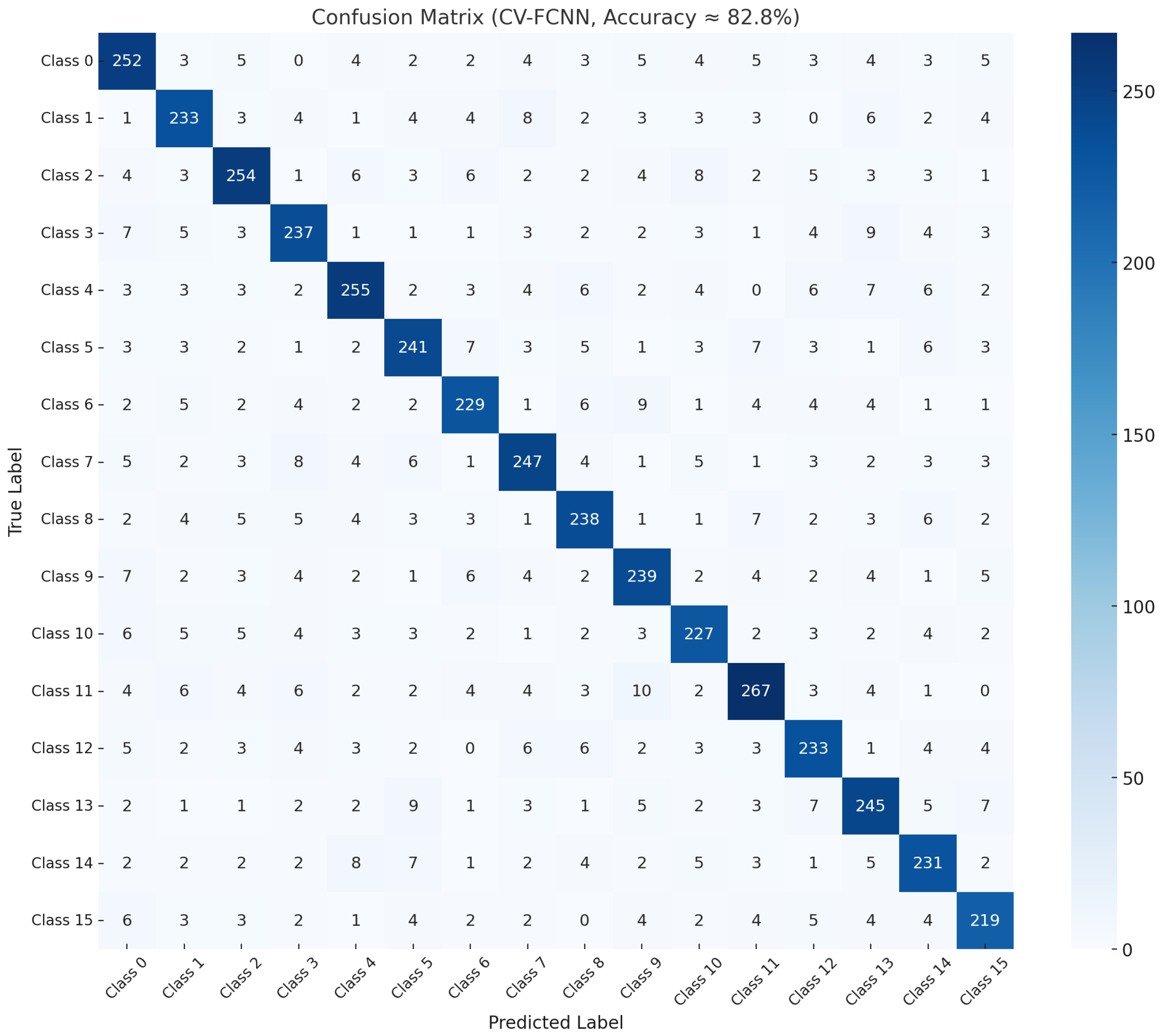
• A defect classification model based on CV-CNN is designed and implemented, achieving superior accuracy and robustness in classifying 16 defect categories, with an overall accuracy of 85.0%, significantly outperforming the complex-valued fully CNN (CV-FCNN) model.
• The complex-valued convolutional architecture jointly models magnitude and phase information, with a specially introduced magnitude pooling strategy, improving the model’s ability to distinguish similar defects and resist noise, thereby enhancing the reliability of practical industrial inspection. The application of the complex-valued neural network (CVNN) provides a novel perspective for eddy current signal processing.

The remainder of this paper is organized as follows. Section 2 reviews the related work on complex-valued neural networks (CVNNs) and their applications in processing complex-valued signals. Section 3 describes the Materials and Methods, including the experimental setup, dataset, architecture, and training and evaluation details. Section 4 presents the Results, including signal measurement results, defect reconstruction, and performance evaluation using precision, recall, and the F1-score, along with a comparison against CV-FCNN. Section 5 discusses the experimental results, analyzes the limitations and applicable scope of this study, and reflects on its practical implications. Section 6 concludes the paper by summarizing the main contributions and outlining directions for future research.

2. Related Work

CVNNs have attracted increasing attention due to their ability to preserve both magnitude and phase information in complex-domain signals, making them particularly advantageous in signal reconstruction, classification, and prediction tasks across various domains.

2.1. MRI Image Reconstruction

In the domain of medical imaging, CNNs have demonstrated rapid and robust performance in magnetic resonance imaging (MRI) reconstruction from undersampled data. Although MRI data is inherently complex-valued, most traditional deep learning frameworks operate in the real domain, leading to a loss of important phase information. To address this issue, researchers have extended common architectures—such as Deep Residual Networks, U-Net [27], and unrolled networks [28]—into the complex domain to form CV-CNNs [29,30,31]. Notably, refs. [29,30] applied complex-valued U-Net architectures and reported that they obtained improved structural similarity index (SSIM) scores compared to their real-valued counterparts and conventional methods. Deep complex MRI [31], a residual-based CVNN, further improves reconstruction quality with an SSIM of 0.920, exceeding the 0.907 achieved by the U-Net in [29]. This approach also reduces the sensitivity to auto-calibration signal (ACS) lines and reconstructs MRI images with less noise at higher acceleration rates than existing parallel imaging techniques.

2.2. Signal Classification and Speech Processing

CVNNs have also been proven effective in signal classification tasks, particularly when dealing with complex-domain inputs such as electromagnetic, optical, sonar, and radio frequency signals [32]. The inherent phase and amplitude components of these signals make CVNNs more suitable than real-valued networks (RVNNs). For instance, a complex wavelet neural network (CWNN) was used in sonar echo classification and solar irradiation forecasting, achieving superior performance by leveraging wavelet activation functions [33]. Further, [34] introduced sparse Fourier feature extraction prior to CWNN classification, outperforming traditional Fourier transform methods. Fully CWNN-based models also achieved enhanced accuracy in solar forecasting by effectively learning correlations between real and imaginary components [35].

In speech applications, CVNNs are leveraged to process acoustic signals by capturing both phase and magnitude. Tsuzuki et al. [36] developed a sound localization system using FFT and CVNNs, while [37] demonstrated that complex-valued U-Net outperforms conventional models in speech enhancement. Hayakawa et al. [38] introduced a hybrid acoustic model incorporating complex-valued layers with a batch amplitude mean normalization strategy, which improved training stability and robustness under noisy conditions. However, Drude et al. [39] reported that a direct, unoptimized extension of RVNNs into the complex domain yielded no significant performance gains, highlighting the need for task-specific CVNN design. Additionally, CVNNs have been utilized in voice-based Parkinson’s disease detection. Methods such as Mc-FCRBF [40], feature selection with mRMR [41], and feature weighting with KMC [42] have collectively improved classification accuracy to as high as 99.52%.

2.3. Broader Applications of CVNNs

Beyond imaging and signal classification, CVNNs have been effectively employed in diverse prediction tasks. These include protein secondary structure prediction, financial time series forecasting, soil moisture estimation, and audio signal prediction to enhance MP3 compression. For instance, the multilayer multivalued neuron model (MLMVN) is used for soil moisture prediction [43], the fully complex-valued recurrent network (FCRN) is applied in protein structure analysis [44], and the complex-valued functional neural tree (CVFNT) is adopted in financial forecasting [45], with optimization via genetic and artificial bee colony algorithms. The integration of CVNN modules into MP3 encoders enables better compression ratios while preserving audio quality [46].

CVNNs have also found utility in specialized tasks such as organic compound classification using Boolean logic-based complex neurons [47], forgery detection in medical imaging [48], and solving complex-valued linear equations [49]. On the hardware side, Zhang et al. [50] demonstrated an optical neural chip that executes complex arithmetic via optical interference. Their optical CVNN implementation effectively handled handwriting recognition and classification tasks, suggesting its future relevance in optical and quantum-inspired computing systems.

In summary, CVNNs have demonstrated substantial advantages in preserving complex signal characteristics and improving task performance across multiple domains, including image reconstruction, signal classification, biomedical diagnosis, and time-series prediction. These findings motivate further exploration of CVNN-based architectures for complex-domain tasks. Unlike many existing CVNN architectures adapted for MRI or speech processing tasks, the CV-CNN model proposed in this study is specifically designed for eddy current signal analysis, where the magnitude and phase components are closely related to defect characteristics. In particular, a magnitude-based max pooling strategy is introduced to enhance local defect features and suppress background noise, differing from conventional CVNNs that often treat magnitude and phase symmetrically or adopt generic pooling approaches.

3. Materials and Methods

3.1. Experimental Setup

In this study, an artificial electrical discharge machining (EDM) notch specimen was employed for eddy current testing. The specimen was made of carbon steel, as shown in Figure 1, with the surface treated to remove mill scale in order to reduce surface interference and improve the signal-to-noise ratio (SNR). The size of the indentation is shown schematically in Figure 2. The overall dimensions of the specimen were 400 mm × 100 mm × 20 mm (length × width × thickness). The length is denoted as L, the width as W, and the thickness as T in Figure 2. Multiple standardized EDM notches were fabricated on the surface to simulate cracks or grooves. Each notch had a fixed width of 0.1 mm, with depths of 0.5 mm, 1.0 mm, 2.0 mm, and 3.0 mm and lengths of 2 mm, 3 mm, 5 mm, 10 mm, and 20 mm. These defects were regularly arranged on the specimen surface to facilitate systematic data acquisition and classification experiments. The scanning area was defined as 100 mm × 30 mm, and a two-dimensional grid scanning strategy was adopted. The X-direction had a scanning step of 0.5 mm for a total of 200 steps, while the Y-direction had an interval of 1.0 mm for 30 lines. A pancake coil was used for detection, with a diameter of 6 mm, consisting of 9 turns per layer and 4 layers, totaling 36 turns. The coil had a thickness of 1.4 mm. To obtain high-quality eddy current signals, the coil was positioned with nearly zero lift-off, meaning that the coil substrate was placed directly onto the surface of the flat specimen. This configuration provides a standardized and repeatable experimental basis for defect detection and characterization. In addition to the 3 mm length defects, the different lengths and depths of the other defects constituted the different types of defects, totaling 16 types, i.e., class 0 to class 15.

3.2. Dataset

The dataset used in this study contains 46,000 eddy current inspection signal samples collected by the Nondestructive Testing and Evaluation Laboratory of Kyoto University, Japan. The specimens were carbon steel blocks with artificially introduced defects, precisely fabricated by electrical discharge machining (EDM) to simulate crack-type defects of varying depths and orientations encountered in practice. Eddy current signals were acquired using a pancake coil probe under four excitation frequencies of 5 kHz, 20 kHz, 80 kHz, and 320 kHz to achieve penetration detection at different depth ranges. Each signal represents the impedance response at a discrete location on the specimen surface. The dataset was divided approximately in the ratio of 7:2:1 into training, validation, and testing sets, consisting of 32,195, 9200, and 4605 samples, respectively. It includes 16 defect types with variations in depth and size, and the sample distribution of the testing set for each defect category is presented in

Table 1. Distribution of sample counts for each defect type.

Defect Category	Number of Defect Samples
Class 0	304
Class 1	281
Class 2	307
Class 3	286
Class 4	308
Class 5	291
Class 6	277
Class 7	298
Class 8	287
Class 9	288
Class 10	274
Class 11	322
Class 12	281
Class 13	296
Class 14	279
Class 15	265

. Each signal is represented in complex form, encompassing variations in both the real and imaginary components of the impedance.

3.3. Network Architecture

CNNs were first introduced in 1990 for handwritten digit recognition [51] and have since been widely applied in various fields such as computer vision [52], autonomous driving [53], and image recognition and classification tasks [54]. Feature extraction and classification are two core components of CNNs. They allow successive layers in the network to learn and discover low-level features and classify them in the final fully connected output layer. Due to their outstanding classification performance, CNNs have been extended to the complex-valued domain, enabling the precise representation of input data in terms of both magnitude and phase [23]. Moreover, complex-valued weights are more stable and numerically efficient in memory access models [55].

The proposed CV-CNN in this work is a neural network with multilayer perception and deep feature extraction capabilities. It typically consists of convolutional layers, pooling layers, and fully connected layers [56], as illustrated in Figure 3.

3.3.1. Convolutional Layer

Each neuron in a CNN is arranged in a feature map and connected to a set of filters or kernels in the convolutional layer, which consists of weight matrices in the complex-valued domain. These kernels slide across the feature maps and perform convolutions between the input elements and the kernel weights. The resulting convolution is passed through an activation function to compute a new feature map [57].

Convolutional layers act as feature extractors, where each filter captures specific local patterns in the input. They detect edges, colors, and gradient directions, enabling the model to understand input images comprehensively. Due to the spatial correlation in image data [58], the same filter group is shared across the same feature map channel. Important features are typically fixed in certain parts of the image, making it essential to scan with the same filters across different regions.

In CV-CNN, a complex-valued convolution unit is calculated by convolving all output feature maps from the previous layer. A complex-valued number, d, is defined as

$$d=a+ib$$

(1)

$$a=\mathrm{Re}\left(d\right),b=\mathrm{Im}\left(d\right)$$

(2)

where a and b represent the real and imaginary parts of the complex-valued number, respectively.

Instead of applying real-valued convolutions separately to the real and imaginary parts, we perform true complex-valued convolution. Let the complex-valued filter be $W=X+iY$, where X and Y are real-valued filters, and let the complex-valued input be $d=a+ib$. Using the distributive property of convolution [30], this operation becomes

$$W\ast d=(X+iY)\ast (a+ib)=(X\ast a-Y\ast b)+i(Y\ast a+X\ast b)$$

(3)

This convolution can be expressed in matrix form as

$$\left[\begin{array}{c}\mathrm{Re}(W\ast d)\\ \mathrm{Im}(W\ast d)\end{array}\right]=\left[\begin{array}{cc}X& -Y\\ Y& X\end{array}\right]\ast \left[\begin{array}{c}a\\ b\end{array}\right]$$

(4)

To mitigate vanishing gradients and achieve faster convergence, we employ the complex-valued ReLU activation function, defined as

$$\mathrm{ReLU}\left(d\right)=\left\{\begin{array}{cc}d\hfill & \mathrm{if} d\ge 0\hfill \\ 0\hfill & \mathrm{otherwise}\hfill \end{array}\right.$$

(5)

3.3.2. Pooling Layer

The pooling layer, also known as a down-sampling layer, reduces the dimensionality of feature maps and generates a lower-resolution version of the input signal. It also helps eliminate irrelevant details in the signal. The two most common pooling operations are max pooling and average pooling, which compute the maximum or average within a defined filter region.

Since the max operator is not directly defined in the complex-valued domain, max pooling in CV-CNN is performed separately on the real and imaginary components. In this work, we adopt magnitude-based max pooling [25], where the complex-valued numbers are projected into the real domain using $\phi \left(d\right)=\left|d\right|$. The magnitude-based max pooling is defined as

$$arg\underset{d\in \mathrm{patch}}{max}\left|d\right|$$

(6)

$$max(d_1,\dots ,d_n)=max(x_1,\dots ,x_n)+imax(y_1,\dots ,y_n)$$

(7)

where patch is a local region in the feature map, and n is the number of elements in the local region.

3.3.3. Fully Connected Layer

The fully connected layer integrates the features extracted from the convolutional layer and outputs the reconstructed results through softmax logistic regression.

3.4. Training and Evaluation

The model was trained using the Adam optimizer with an initial learning rate of 0.001. The learning rate was maintained constantly throughout the training process, which lasted for 500 epochs. To effectively capture the complex-valued nature of the eddy current signals, the loss function employed was the complex-valued mean squared error (CMSE), defined as

$$L_{CMSE}={\displaystyle \frac{1}{N}}\sum _{i=1}^N\left[{\left(\Re \left({\widehat{z}}_i\right)-\Re \left(z_i\right)\right)}^2+{\left(\Im \left({\widehat{z}}_i\right)-\Im \left(z_i\right)\right)}^2\right]$$

(8)

where ${\widehat{z}}_i$ and $z_i$ represent the predicted and true complex values, respectively, and $\Re (·)$ and $\Im (·)$ denote the real and imaginary parts of the complex numbers.

This loss function enabled the model to simultaneously learn the amplitude and phase features of the signals, thereby improving its representation capability. For model evaluation, several classification metrics derived from the confusion matrix were utilized, including accuracy, precision, recall, and F1-score. Accuracy quantifies the overall correctness of model predictions; precision measures the proportion of true positive predictions among all positive predictions, reflecting the reliability of the model; recall assesses the coverage of actual positive samples correctly identified by the model; and F1-score, the harmonic mean of precision and recall, provides a balanced evaluation especially in cases of class imbalance. These metrics are widely adopted in defect detection tasks to comprehensively assess models’ performance.

4. Results

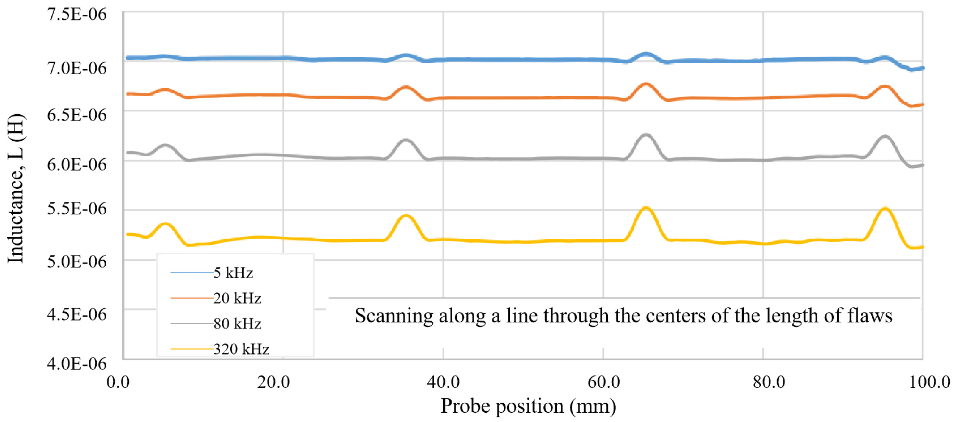
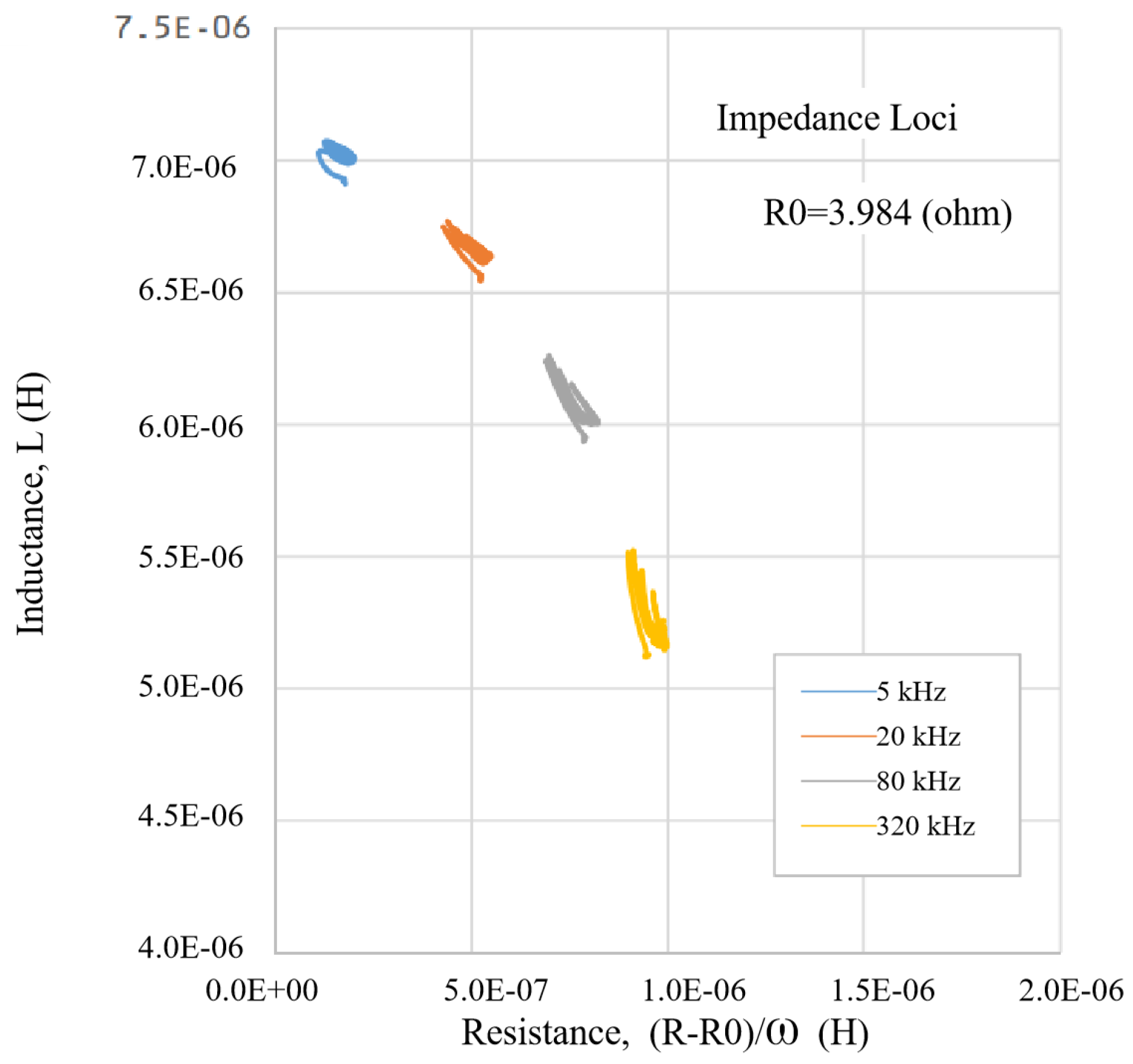
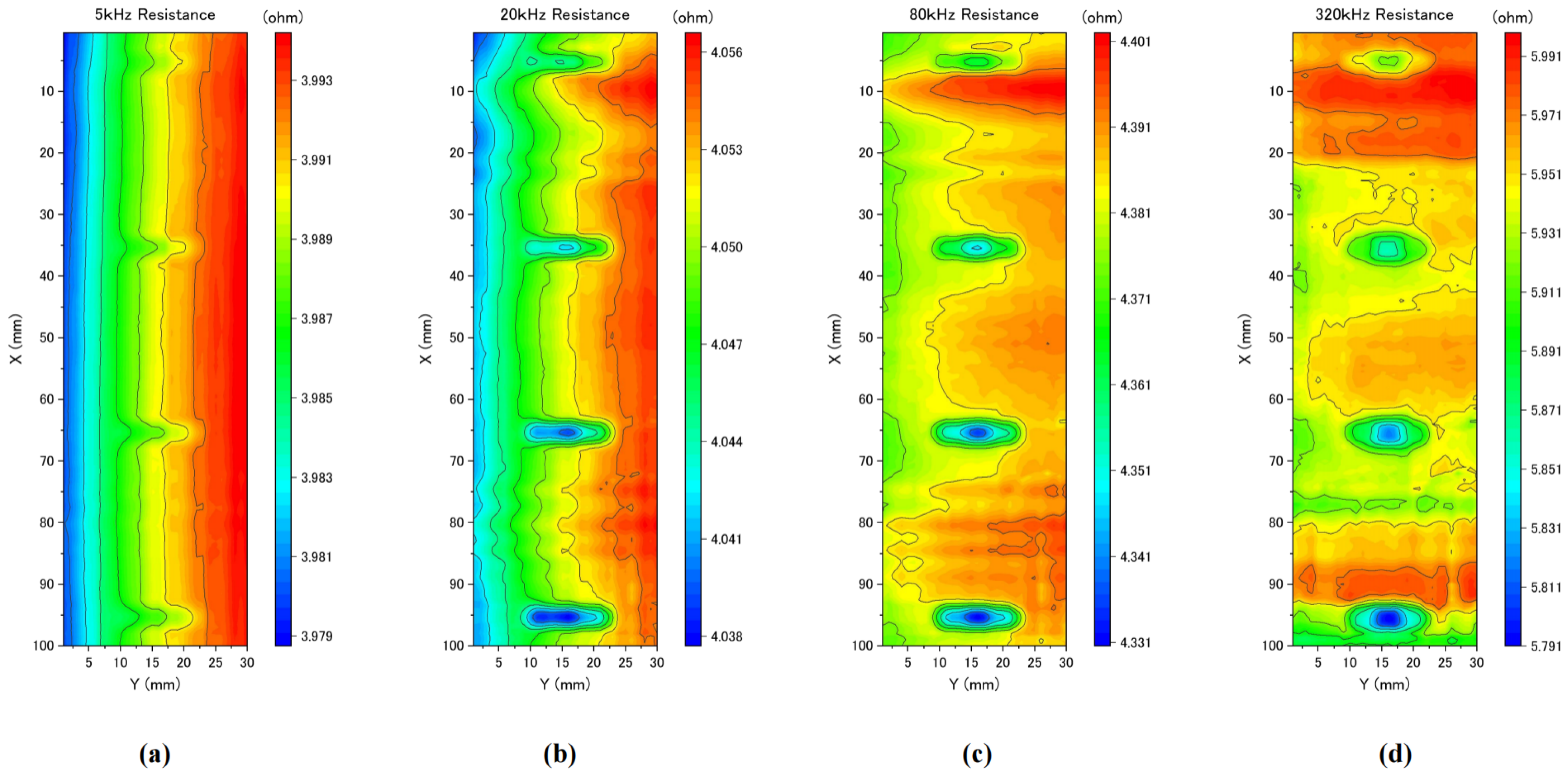
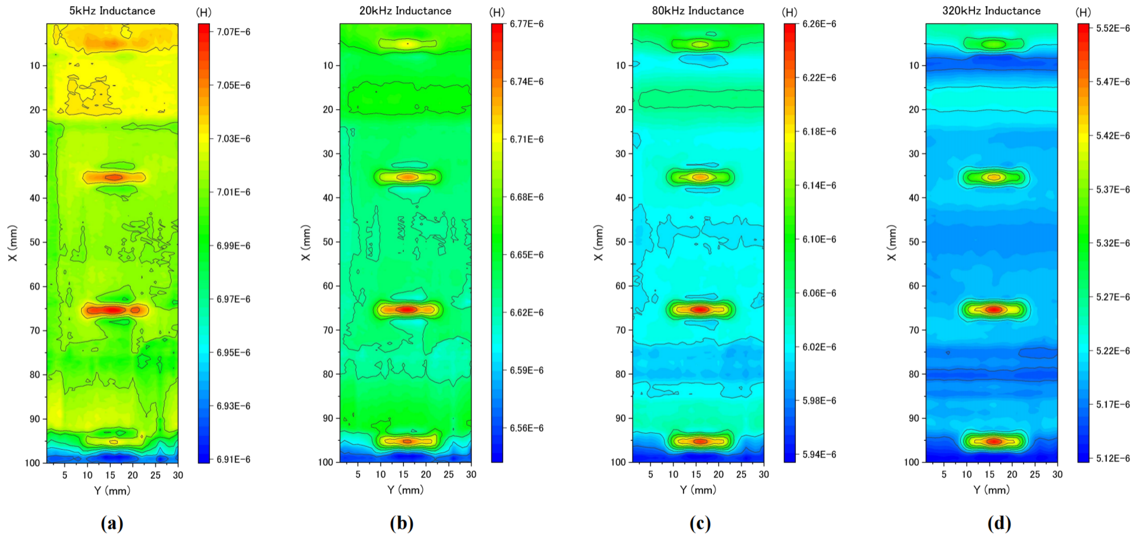
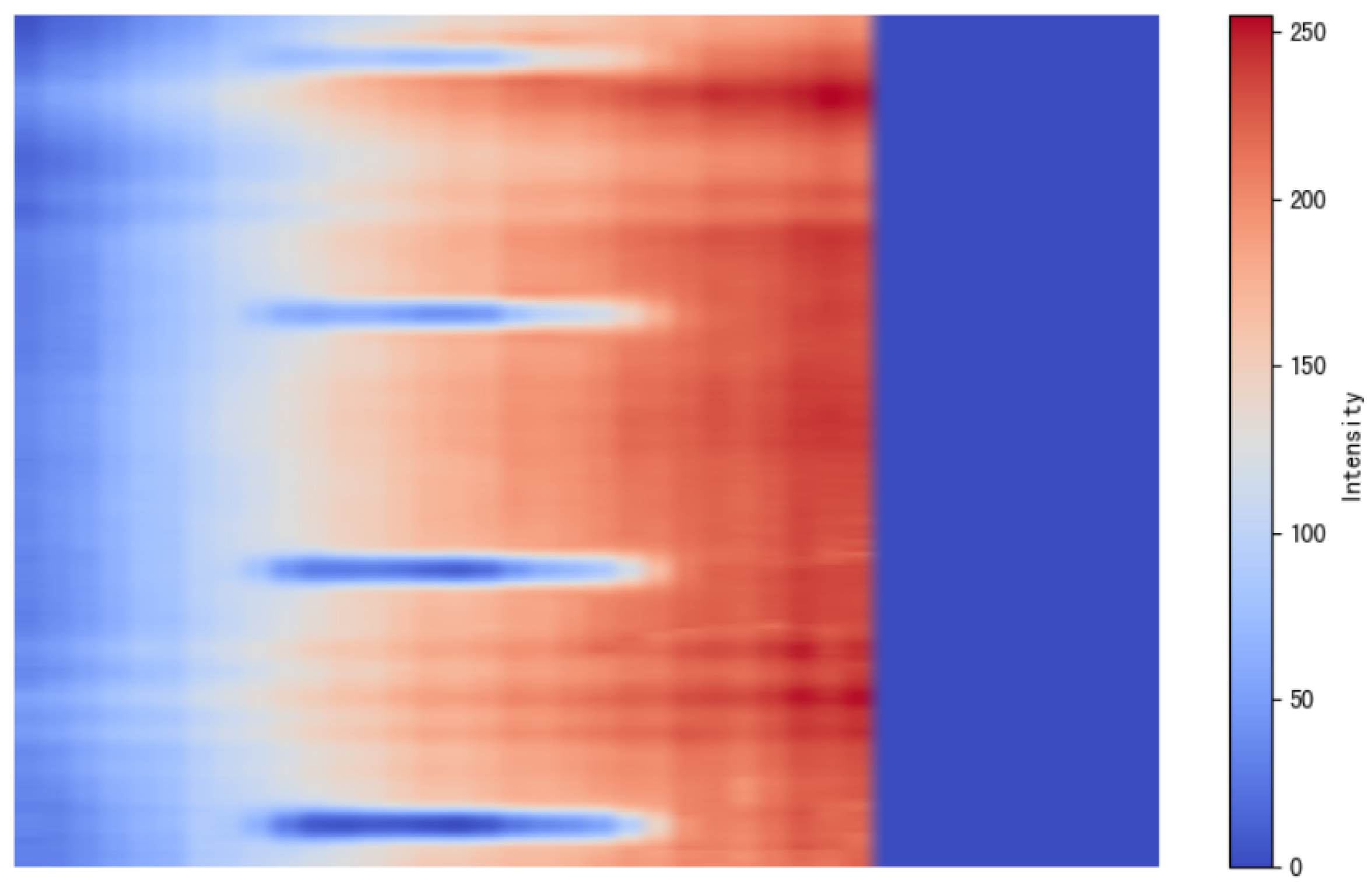
4.1. Measured Signal Results

As a presentation of the results of the measured signals, Figure 4, Figure 5 and Figure 6 present the centerline scan results from the eddy current testing on a carbon steel specimen. The flaw was a 10 mm long EDM notch with depths of 0.5 mm, 1.0 mm, 2.0 mm, and 3.0 mm. A total of 46,000 complex-valued signal samples were collected from eddy current testing on carbon steel plates using four excitation frequencies: 5 kHz, 20 kHz, 80 kHz, and 320 kHz. The dataset was subsequently divided into training, validation, and test sets in a 7:2:1 ratio.

Figure 4 shows how the resistance (real part of impedance) changed with the probe position X at different frequencies. A clear increase or peak in resistance appeared when the probe scanned across the flaw region (approximately 40–60 mm). Low-frequency signals (5 kHz) resulted in broader, smoother responses, while high-frequency (320 kHz) signals produced sharp and localized peaks, suitable for surface flaw characterization.

Figure 5 shows the variation in inductance (imaginary part of impedance) with position. The flaw caused a localized reduction in inductance, appearing as a clear dip in the response. At higher frequencies (e.g., 320 kHz), the change was more focused and accurate for flaw localization, while lower frequencies (e.g., 5 kHz) provided broader responses that better penetrated deeper flaws.

Figure 6 uses $(R-R_0)/\omega$ as the horizontal axis and L as the vertical axis to illustrate the phase trajectory of complex-valued impedance during the scan. where R0 is the carbon steel resistance when no bias magnetic field was applied. Different frequencies formed distinct trajectory shapes. High-frequency traces were shorter and steeper, indicating higher sensitivity to surface-breaking flaws, whereas low-frequency curves were smoother, offering better penetration and depth characterization.

4.2. Defect Reconstruction Results

For defect diameters of 10 mm in length, both in the inductive and resistive components, the results are shown in Figure 7 and Figure 8.

In the inductive component, as shown in Figure 7, the defect signals became clearer as the excitation frequency gradually increased; especially at the low frequency of 5 kHz, the defects with a depth of 0.5 mm were not detected effectively, which indicates that the sensitivity of the low frequency to such defects is poor. As the frequency increased, especially at 80 kHz and 320 kHz, the defect signals were significantly enhanced to detect defects of all depths, and the clarity of the defect signals gradually improved as the excitation frequency increased. This indicates that the high-frequency eddy currents are more sensitive to small defects and are able to more accurately detect tiny defects on the surface and in shallow superficial layers.

In the resistive component, as shown in Figure 8, at an excitation frequency of 5 kHz, the signals of the smallest defects were relatively weak and almost undetectable. However, as the excitation frequency increased, the detection of defect signals improved significantly, especially at 80 kHz and 320 kHz, where all defects could be detected and the signals showed clearer fluctuations, suggesting that these frequencies were more suitable for detecting defects in the middle to shallow layers.

Figure 9 presents the reconstructed defect images for a 10 mm flaw at 5 kHz. Compared with the original eddy current signal maps, the reconstructed results exhibit significantly enhanced defect features, indicating that the proposed method greatly improves defect visualization and recognition. The background noise is effectively suppressed, and the defect boundaries appear much sharper, resulting in clearer and more accurate shape contours. This improvement is particularly important for nondestructive evaluation applications, where the precise geometric characterization of defects is crucial for assessing structural integrity. Moreover, the reconstructed images reveal more defined internal defect structures, which are often obscured in raw impedance maps due to signal distortion or interference. This implies that the complex-valued convolutional operations successfully capture essential morphological details from both the amplitude and phase components. In addition, the inter-class differences among various types of flaws become more distinguishable in the reconstructed feature space. Subtle variations in size, orientation, and depth are more clearly represented, facilitating better separation and recognition by the downstream classification model. These enhancements not only benefit the visual interpretability of defect maps but also increase the model’s discriminative ability across multiple defect types. Overall, the results demonstrate the effectiveness of the proposed CV-CNN-based reconstruction in generating high-fidelity and diagnostically meaningful representations of eddy current signals.

4.3. Reconstruction Performance Evaluation

To evaluate the classification performance of the proposed method in eddy current signal-based defect detection, we compare the confusion matrices of the proposed CV-CNN and CV-FCNN, as shown in Figure 10 and Figure 11, respectively. These matrices provide visual insights into the predictive accuracy and inter-class confusion behavior across different defect types. The proposed CV-CNN achieved an overall classification accuracy of 85.0%, outperforming CV-FCNN, which attained 82.8%. This 2.2 percentage point improvement demonstrates the superiority of CV-CNN in distinguishing defect patterns from eddy current signals. A deeper analysis of the confusion matrices reveals that CV-CNN significantly suppresses inter-class confusion, as evidenced by the generally higher diagonal elements and more concentrated misclassifications. In contrast, CV-FCNN exhibits greater dispersion in off-diagonal entries, especially among similar defect types. This performance gap is primarily due to the difference in network structure. The fully connected layers of CV-FCNN tend to oversmooth local features, making it more susceptible to confusion between neighboring classes. In contrast, the convolutional structure of CV-CNN effectively preserves spatial–temporal locality within the signal, capturing subtle but critical features of defect signatures.

In conclusion, the confusion matrix analysis confirms that the proposed CV-CNN not only improves overall classification accuracy but also enhances robustness against noise and inter-class similarity. These results highlight the effectiveness of convolutional modeling in complex-valued domains for industrial non-destructive testing applications.

To further evaluate the classification performance of the proposed CV-CNN model, a comparative experiment was conducted against a baseline CV-FCNN. Both models were trained and tested on the same dataset under identical conditions to ensure fairness and consistency. The comparison focuses on key evaluation metrics including precision, recall, F1-score, and overall accuracy.

The comparative results are summarized in

Table 2. Comparison of classification metrics between CV-CNN and CV-FCNN.

Category	CV-FCNN			CV-CNN
	Precision	Recall	F1-Score	Precision	Recall	F1-Score
Class 0	0.7926	0.8258	0.8089	0.8562	0.8730	0.8645
Class 1	0.8021	0.7909	0.7965	0.8357	0.8505	0.8430
Class 2	0.8512	0.8571	0.8542	0.8305	0.8140	0.8221
Class 3	0.8303	0.7986	0.8142	0.8810	0.8287	0.8541
Class 4	0.8561	0.8264	0.8410	0.8442	0.8525	0.8483
Class 5	0.8310	0.8397	0.8354	0.8304	0.8188	0.8246
Class 6	0.8013	0.8542	0.8269	0.8500	0.8561	0.8530
Class 7	0.8321	0.8090	0.8204	0.8767	0.8649	0.8707
Class 8	0.8442	0.8118	0.8277	0.8392	0.8362	0.8377
Class 9	0.8259	0.8432	0.8345	0.8305	0.8566	0.8434
Class 10	0.8432	0.8403	0.8417	0.7803	0.8408	0.8094
Class 11	0.8696	0.8362	0.8526	0.8954	0.8589	0.8768
Class 12	0.8201	0.8201	0.8201	0.8720	0.8842	0.8780
Class 13	0.8305	0.8362	0.8333	0.8562	0.8418	0.8489
Class 14	0.8467	0.8438	0.8452	0.8587	0.8556	0.8571
Class 15	0.8133	0.8502	0.8313	0.8571	0.8669	0.8620

. It is evident that the CV-CNN model outperformed CV-FCNN in most performance indicators. Specifically, CV-CNN achieved an overall classification accuracy of 85.00%, which was approximately 2 percentage points higher than the CV-FCNN’s 82.80%.

In terms of per-class metrics, CV-CNN exhibited higher F1-scores in 12 out of 16 defect types, suggesting superior and more stable classification capability. Notably, for several critical defect categories such as Class 0, Class 3, Class 7, and Class 12, CV-CNN achieved significant improvements in both precision and recall, resulting in overall better F1 performance. For instance, the F1-score for Class 3 reached 0.8541 for CV-CNN, compared to 0.8142 for CV-FCNN. These improvements can be attributed to the model’s ability to exploit both amplitude and phase information from complex-valued eddy current signals, particularly with the use of magnitude-based pooling.

In summary, the comparison in Table 2 confirms the superior classification performance and robustness of the proposed CV-CNN model.

5. Discussion

The use of a CV-CNN brings unique advantages in modeling both magnitude and phase information simultaneously. This is particularly important in eddy current testing, where defect characteristics are embedded in complex-valued impedance patterns. Compared to real-valued CNNs, CV-CNN better captures subtle feature differences, leading to higher classification performance and clearer reconstructed images.

From the perspective of model structure and data characteristics, CV-CNN effectively leverages the complex-valued nature of eddy current signals to jointly extract amplitude and phase features, showing strong adaptability to crack-type defects. These defects typically exhibit directional and coherent responses in the complex plane, which aligns well with the feature learning capacity of CV-CNN.

In terms of methodological innovation, CV-CNN goes beyond the limitations of traditional real-valued architectures by incorporating complex-valued convolution, which significantly enhances its capacity to model phase-dominant features. This complex-valued modeling framework offers a novel approach for deep feature extraction and the decision analysis of eddy current signals, thus opening new avenues for signal processing in nondestructive testing. From the perspective of limitations, the current model primarily targets defects with clear structures and concentrated forms, such as cracks. For diffuse, irregular, or composite defects (such as corrosion or coexisting cracks and corrosion), its identification capabilities require further validation. Such defects often lack regular amplitude–phase structures in eddy current responses, which can lead to reduced model generalization capabilities. Future efforts could explore incorporating more representative data, conducting cross-domain feature fusion, or constructing spatio-temporal hybrid structures to enhance the model’s ability to identify complex defects.

Despite these challenges, the current experimental results have fully demonstrated the application value of CV-CNN in crack-oriented defect recognition tasks, showing its potential for deployment in real-world NDT systems, especially in industries that demand high accuracy in early crack detection, such as aircraft maintenance, rail transit, and energy equipment inspection.

In terms of future application, CV-CNN is well-suited for high-precision crack detection in industrial settings. Its lightweight structure facilitates integration with embedded sensing systems and allows further expansion toward smart inspection solutions incorporating digital twins and industrial IoT platforms, promoting the intelligent and adaptive evolution of nondestructive testing technologies.

6. Conclusions

This paper presents a defect reconstruction and classification method based on CV-CNN, which effectively exploits both amplitude and phase information in eddy current signals. Comparative experiments with the conventional CV-FCNN model validate the superiority of the proposed method. The following major conclusions are drawn:

• CV-CNN significantly enhances the representation of defect features, providing clearer and more distinguishable signals under varying excitation frequencies, greatly improving the visualization and interpretability of the signals;
• Compared with CV-FCNN, CV-CNN achieves higher overall accuracy (85.0%) and effectively suppresses inter-class confusion. By preserving local features in complex-valued signals, CV-CNN demonstrates stronger stability and robustness, achieving higher precision, recall, and F1-scores across multiple key defect categories.

In summary, the proposed CV-CNN-based method not only achieves superior performance in defect reconstruction but also demonstrates high accuracy and generalization in the classification of complex eddy current signals, offering a promising solution for industrial NDT.

Future work will focus on constructing a complex defect dataset with overlapping types, designing more robust CVNN architectures to accommodate signal coupling, and enhancing CV-CNN’s generalization and representation in ECT modeling through augmented samples and physical priors.

References

1. Machado, M.A. Eddy currents probe design for NDT applications: A review. Sensors 2024, 24, 5819. [Google Scholar] [CrossRef] [PubMed]
2. Wrzuszczak, M.; Wrzuszczak, J. Eddy current flaw detection with neural network applications. Measurement 2005, 38, 132–136. [Google Scholar] [CrossRef]
3. Zhou, X.; Urayama, R. Application of back-propagation neural networks to defect characterization using eddy current testing. Int. J. Appl. Electron. 2020, 64, 817–825. [Google Scholar] [CrossRef]
4. Rao, B.P.C.; Raj, B. A new approach for restoration of eddy current images. J. Nondestruct. Eval. 2001, 20, 61–72. [Google Scholar] [CrossRef]
5. Hu, J.; Zhang, Z.; Ding, Z.; Lin, Y.; Zhou, X.; Zhu, G. Multi-Task Learning in eddy current testing of spherical tank arrays: Defect detection and classification. In Proceedings of the 2024 4th International Conference on Mobile Networks and Wireless Communications (ICMNWC), Tumkuru, India, 4–5 December 2024. [Google Scholar]
6. D’Angelo, G.; Laracca, M.; Rampone, S.; Betta, G. Fast eddy current testing defect classification using lissajous figures. IEEE Trans. Instrum. Meas. 2018, 67, 821–830. [Google Scholar] [CrossRef]
7. Lysenko, I.; Kuts, Y.; Uchanin, V.; Mirchev, Y.; Levchenko, O. Evaluation of eddy current array performance in detecting aircraft component defects. Trans. Aerosp. Res. 2024, 275, 1–9. [Google Scholar] [CrossRef]
8. Xu, D.; Hou, H.S.; Liu, C.X.; Jiao, C. Defect type identification of thin-walled stainless steel seamless pipe based on eddy current testing. Insight 2021, 63, 697–703. [Google Scholar] [CrossRef]
9. Fan, M.; Wang, Q.; Cao, B.; Ye, B.; Sunny, A.I.; Tian, G. Frequency optimization for enhancement of surface defect classification using the eddy current technique. Insight 2016, 16, 649. [Google Scholar] [CrossRef]
10. Kumar, N.; Joseyphus, R.J. Eddy current thermography as a tool for detecting the location and dimension of edge defects in Cr–Mo steel plate. In Advances in Non Destructive Evaluation; Springer: Singapore, 2022; pp. 23–40. [Google Scholar]
11. Gao, S.; Zheng, Y.; Li, S.; Zhang, J.; Bai, L.; Ding, Y. Eddy current array for defect detection in finely grooved structure using MSTSA network. Sensors 2024, 24, 6078. [Google Scholar] [CrossRef]
12. Bernieri, A.; Ferrigno, L.; Laracca, M.; Molinara, M. Crack shape reconstruction in eddy current testing using machine learning systems for regression. IEEE Trans. Instrum. Meas. 2008, 57, 1958–1968. [Google Scholar] [CrossRef]
13. Preda, G.; Hantila, F.I. Nonlinear integral formulation and neural network-based solution for reconstruction of deep defects with pulse eddy currents. IEEE Trans. Magn. 2014, 50, 113–116. [Google Scholar] [CrossRef]
14. Betta, G.; Ferrigno, L.; Laracca, M.; Ramos, H.G.; Ricci, M.; Ribeiro, A.L. Fast 2D crack profile reconstruction by image processing for eddy current testing. In Proceedings of the 2015 IEEE Metrology for Aerospace (MetroAeroSpace), Benevento, Italy, 4–5 June 2015; pp. 23–40. [Google Scholar]
15. Abderrahmane, A.; Abdelhak, A.; Tarik, B.; Mohamed, C.; Bachir, A.; Merwane, K. Reconstruction of defect paths using eddy current testing array 3D imaging. Electr. Mech. Eng. 2024, 16, 38–47. [Google Scholar] [CrossRef]
16. Benissad, S.; Touati, M.; Chabaat, M. Artificial neural networks for inverse problems in damage detection using computational and experimental eddy current. Period. Polytech. Civ. Eng. 2023, 67, 1–9. [Google Scholar] [CrossRef]
17. Yusa, N.; Machida, E.; Janousek, L.; Rebican, M.; Chen, Z.; Miya, K. Application of eddy current inversion technique to the sizing of defects in Inconel welds with rough surfaces. Nucl. Eng. Des. 2005, 235, 1469–1480. [Google Scholar] [CrossRef]
18. Li, M.; Lowther, D.; Guimar, F. Robust and accurate crack reconstruction for eddy current non destructive testing. Int. J. Appl. Electromagn. Mech. 2014, 45, 425–430. [Google Scholar] [CrossRef]
19. Ahn, Y.S.; Gil, D.S.; Park, S.G. The Design & Manufacture and characteristic analysis of eddy current sensor for bolt hole defect evaluation. J. Power Syst. Eng. 2011, 15, 37–41. [Google Scholar]
20. Zhang, K.; Dong, Z.; Yu, Z.; He, Y. Shape mapping detection of electric vehicle alloy defects based on pulsed eddy current rectangular sensors. Appl. Sci. 2018, 8, 2066. [Google Scholar] [CrossRef]
21. Cheng, W.; Komura, I.; Shiwa, M.; Kanemoto, S. Eddy current examination of fatigue cracks in inconel welds. J. Press. Vessel Technol. 2007, 129, 169–174. [Google Scholar] [CrossRef]
22. Barrarat, F.; Rayane, K.; Helifa, B.; Chettouh, B.; Lefkaier, I.K. Reconstruction of defect size and shape in eddy-current testing using benchmark problems validation and neural network approach. Malays. J. Fundam. Appl. Sci. 2020, 12, 78–88. [Google Scholar]
23. Cole, E.; Cheng, J.; Pauly, J.; Vasanawala, S. Analysis of deep complex-valued convolutional neural networks for MRI reconstruction and phase-focused applications. Magn. Reson. Med. 2021, 86, 1093–1109. [Google Scholar] [CrossRef]
24. Chatterjee, S.; Tummala, P.; Speck, O.; Nurnberger, A. Complex network for complex problems: A comparative study of cnn and complex-valued cnn. In Proceedings of the 2022 IEEE 5th International Conference on Image Processing Applications and Systems (IPAS), Genova, Italy, 5–7 December 2022; pp. 1–5. [Google Scholar]
25. Lee, C.Y.; Hasegawa, H.; Gao, S. Complex-valued neural networks: A comprehensive survey. IEEE/CAA J. Autom. Sin. 2022, 9, 1406–1426. [Google Scholar] [CrossRef]
26. Li, S.; Zhang, L.; Guo, H.; Li, J.; Yu, J.; He, X. CSA-FCN: Channel-and spatial-gated attention mechanism based fully complex-valued neural network for system matrix calibration in magnetic particle imaging. IEEE Trans. Comput. Imaging 2025, 11, 65–76. [Google Scholar] [CrossRef]
27. Ronneberger, O.; Fischer, P.; Brox, T. U-net: Convolutional networks for biomedical image segmentation. In Proceedings of the Medical Image Computing and Computer-Assisted Intervention—MICCAI 2015: 18th International Conference, Munich, Germany, 5–9 October 2015; pp. 234–241. [Google Scholar]
28. Diamond, S.; Sitzmann, V.; Heide, F.; Wetzstein, G. Unrolled optimization with deep priors. arXiv 2018, arXiv:1705.08041. [Google Scholar]
29. Dedmari, M.A.; Conjeti, S.; Estrada, S.; Ehses, P.; Stöcker, T.; Reuter, M. Complex Fully Convolutional Neural Networks for MR Image Reconstruction. In Proceedings of the 1st Workshop on Machine Learning for Medical Image Reconstruction (MLMIR) Held as Part of the 21st Conference on Medical Image Computing and Computer Assisted Intervention (MICCAI), Granada, Spain, 16–20 September 2018; pp. 1231–1236. [Google Scholar]
30. Cole, E.K.; Pauly, J.; Cheng, J. Complex-valued convolutional neural networks for MRI reconstruction. In Proceedings of the 27th Annual Meeting of ISMRM, Montreal, QC, Canada, 11–16 May 2019; 4714. [Google Scholar]
31. Wang, S.; Cheng, H.; Ying, L.; Xiao, T.; Ke, Z.; Zheng, H. DeepcomplexMRI: Exploiting deep residual network for fast parallel MR imaging with complex convolution. Magn. Reson. Imaging 2020, 68, 136–147. [Google Scholar] [CrossRef]
32. Hirose, A.; Nakane, R.; Tanaka, G. Keynote speech: Information processing hardware, physical reservoir computing and complex-valued neural networks. In Proceedings of the 2019 IEEE International Meeting for Future of Electron Devices, Kansai (IMFEDK), Kyoto, Japan, 14–15 November 2019; pp. 19–24. [Google Scholar]
33. Alexandridis, A.K.; Zapranis, A.D. Wavelet neural networks: A practical guide. Neural Netw. 2013, 42, 1–27. [Google Scholar] [CrossRef]
34. Özkan Bakbak, P.; Peker, M. Classification of sonar echo signals in their reduced sparse forms using complex-valued wavelet neural network. Neural Comput. Appl. 2020, 32, 2231–2241. [Google Scholar] [CrossRef]
35. Saad Saoud, L.; Rahmoune, F.; Tourtchine, V.; Baddari, K. Fully complex valued wavelet network for forecasting the global solar irradiation. Neural Process. Lett. 2017, 45, 475–505. [Google Scholar] [CrossRef]
36. Tsuzuki, H.; Kugler, M.; Kuroyanagi, S.; Iwata, A. An approach for sound source localization by complex-valued neural network. IEICE Trans. Inf. Syst. 2013, 96, 2257–2265. [Google Scholar] [CrossRef]
37. Choi, H.-S.; Kim, J.-H.; Huh, J.; Kim, A.; Ha, J.-W.; Lee, K. Phase-aware speech enhancement with deep complex u-net. In Proceedings of the International Conference on Learning Representations, New Orleans, LA, USA, 6–9 May 2019. [Google Scholar]
38. Hayakawa, D.; Masuko, T.; Fujimura, H. Applying complex-valued neural networks to acoustic modeling for speech recognition. In Proceedings of the 2018 Asia-Pacific Signal and Information Processing Association Annual Summit and Conference (APSIPA ASC), Honolulu, HI, USA, 12–15 November 2018. [Google Scholar]
39. Drude, L.; Raj, B.; Haeb-Umbach, R. On the Appropriateness of Complex-Valued Neural Networks for Speech Enhancement. In Proceedings of the Interspeech, San Francisco, CA, USA, 8–12 September 2016. [Google Scholar]
40. Gokul, S.; Sivachitra, M.; Vijayachitra, S. Parkinson’s disease prediction using machine learning approaches. In Proceedings of the 2013 Fifth International Conference on Advanced Computing (ICoAC), Chennai, India, 18–20 December 2013. [Google Scholar]
41. Peker, M.; Şen, B.; Delen, D. Computer-Aided Diagnosis of Parkinson’s Disease Using Complex-Valued Neural Networks and mRMR Feature Selection Algorithm. J. Healthc. Eng. 2015, 6, 281–302. [Google Scholar] [CrossRef]
42. Gürüler, H. A novel diagnosis system for Parkinson’s disease using complex-valued artificial neural network with k-means clustering feature weighting method. Neural Comput. Appl. 2017, 28, 1657–1666. [Google Scholar] [CrossRef]
43. Ji, R.; Zhang, S.; Zheng, L.; Liu, Q.; Saeed, I.A. Prediction of soil moisture with complex-valued neural network. In Proceedings of the 2017 29th Chinese Control And Decision Conference (CCDC), Chongqing, China, 28–30 May 2017; pp. 1231–1236. [Google Scholar]
44. Rashid, S.; Saraswathi, S.; Kloczkowski, A.; Sundaram, S.; Kolinski, A. Protein secondary structure prediction using a small training set (compact model) combined with a Complex-valued neural network approach. BMC Bioinform. 2016, 17, 362. [Google Scholar] [CrossRef] [PubMed]
45. Yang, B.; Zhang, W.; Gong, L.N.; Ma, H.Z. Finance time series prediction using complex-valued flexible neural tree model. In Proceedings of the 2017 13th International Conference on Natural Computation, Guilin, China, 29–31 July 2017; pp. 54–58. [Google Scholar]
46. Al-Nuaimi, A.Y.H.; Amin, M.F.; Murase, K. Enhancing MP3 encoding by utilizing a predictive complex-valued neural network. In Proceedings of the 2012 International Joint Conference on Neural Networks (IJCNN), Brisbane, QLD, Australia, 10–15 June 2012; pp. 1–6. [Google Scholar]
47. Akhmetsin, R.M.; Giniyatullin, V.M.; Kirlan, S.A. Identification of structures of organic substances by means of complex-valued perceptron. Opt. Mem. Neural Netw. 2012, 21, 11–16. [Google Scholar] [CrossRef]
48. Olanrewaju, R.F.; Khalifa, O.O.; Hashim, A.H.; Zeki, A.M.; Aburas, A.A. Forgery detection in medical images using complex valued neural network (CVNN). Aust. J. Basic Appl. Sci. 2011, 5, 1251–1264. [Google Scholar]
49. Xiao, L.; Meng, W.; Lu, R.; Yang, X.; Liao, B.; Ding, L. A fully complex-valued neural network for rapid solution of complex-valued systems of linear equations. In Proceedings of the Advances in Neural Networks—ISNN 2015: 12th International Symposium on Neural Networks, ISNN 2015, Jeju, Republic of Korea, 15–18 October 2015; pp. 444–451. [Google Scholar]
50. Zhang, H.; Gu, M.; Jiang, X.D.; Thompson, J.; Cai, H.; Paesani, S. An optical neural chip for implementing complex-valued neural network. Nat. Commun. 2021, 12, 457–458. [Google Scholar] [CrossRef] [PubMed]
51. Cun, Y.L.; Boser, B.; Denker, J.S.; Henderson, D.; Jackel, L.D. Handwritten digit recognition with a back-propagation network. Adv. Neural Inf. Process. Syst. 1990, 2, 396–404. [Google Scholar]
52. Lecun, Y.; Kavukcuoglu, K.; Clément, F. Convolutional networks and applications in vision. In Proceedings of the 2010 IEEE International Symposium on Circuits and Systems, Paris, France, 30 May–2 June 2010; pp. 253–256. [Google Scholar]
53. Kebria, P.; Khosravi, A.; Salaken, S.M.; Nahavandi, S. Deep imitation learning for autonomous vehicles based on convolutional neural networks. IEEE/CAA J. Autom. Sin. 2020, 7, 14–20. [Google Scholar] [CrossRef]
54. Moeskops, P.; Viergever, M.A.; Adriënne, M.M.; Vries, L.S.D.; Benders, M.J.N.L.; Ivana, I. Automatic segmentation of mr brain images with a convolutional neural network. IEEE Trans. Med. Imaging 2016, 35, 1252–1261. [Google Scholar] [CrossRef]
55. Danihelka, I.; Wayne, G.; Uria, B.; Kalchbrenner, N.; Graves, A. Associative Long Short-Term Memory. In Proceedings of the 33rd International Conference on Machine Learning, New York, NY, USA, 9 February 2016; pp. 2256–2977. [Google Scholar]
56. Li, Z.; Liu, F.; Yang, W.; Peng, S.; Zhou, J. A survey of convolutional neural networks: Analysis, applications, and prospects. IEEE Trans. Neural Netw. Learn. Syst. 2021, 33, 6999–7019. [Google Scholar] [CrossRef]
57. Rawat, W.; Wang, Z. Deep convolutional neural networks for image classification: A comprehensive review. Neural Comput. 2017, 29, 2352–2449. [Google Scholar] [CrossRef]
58. LeCun, Y.; Bengio, Y.; Hinton, G. Deep learning. Nature 2015, 521, 436–444. [Google Scholar] [CrossRef]
Figure 1. Carbon steel sample used.
Applsci 15 06599 g001
Figure 2. Schematic diagram of defects in carbon steel.
Applsci 15 06599 g002
Figure 3. The proposed framework of CV-CNN.
Applsci 15 06599 g003
Figure 4. Resistance changes with probe position.
Applsci 15 06599 g004
Figure 5. Inductance changes with probe position.
Applsci 15 06599 g005
Figure 6. Impedance loci.
Applsci 15 06599 g006
Figure 7. Two-dimensional contour plots of pancake coil inductance at different excitation frequencies for EDM recesses with depths from 0.5 mm to 3.0 mm and lengths of 10 mm: (a): 5 kHz; (b): 20 kHz; (c): 80 kHz; (d): 320 kHz.
Applsci 15 06599 g007
Figure 8. Two-dimensional contour plots of pancake coil resistance at different excitation frequencies for EDM recesses with depths from 0.5 mm to 3.0 mm and lengths of 10 mm: (a): 5 kHz; (b): 20 kHz; (c): 80 kHz; (d): 320 kHz.
Applsci 15 06599 g008
Figure 9. Two-dimensional contour plots of pancake coil reconstructed defect image for EDM recesses with depths from 0.5 mm to 3.0 mm and lengths of 10 mm.
Applsci 15 06599 g009
Figure 10. Confusion matrix of the CV-CNN model.
Applsci 15 06599 g010
Figure 11. Confusion matrix of the proposed CV-FCNN model.
Applsci 15 06599 g011