Enhanced Tracking in Legged Robots through Model Reduction and Hybrid Control Techniques: Addressing Disturbances, Delays, and Saturation

Abstract

This study introduces a reduced-order leg dynamic model to simplify the controller design and enhance robustness. The proposed multi-loop control scheme tackles tracking control issues in legged robots, including joint angle and contact-force regulation, disturbance suppression, measurement delay, and motor saturation avoidance. Firstly, model predictive control (MPC) and sliding mode control (SMC) schemes are developed using a simplified model, and their stability is analyzed using the Lyapunov method. Numerical simulations under two disturbances validate the superior tracking performance of the SMC scheme. Secondly, an Nth-order linear active disturbance rejection control (LADRC) is designed based on a simplified model and optimization problems. The second-order LADRC-SMC scheme reduces the contact-force control error in the SMC scheme by ten times. Finally, a fourth-order LADRC-SMC with a Smith Predictor (LADRC-SMC-SP) scheme is formulated, employing each loop controller independently. This scheme simplifies the design and enhances performance. Compared to numerical simulations of the above and existing schemes, the LADRC-SMC-SP scheme eliminates delay oscillations, shortens convergence time, and demonstrates fast force-position tracking responses, minimal overshoot, and strong disturbance rejection. The peak contact-force error in the LADRC-SMC-SP scheme was ten times smaller than that in the LADRC-SMC scheme. The integral square error (ISE) values for the tracking errors of joint angles ${\theta }_1$and ${\theta }_2$, and contact force $f$, are $1.6636\times 10^{-28} \mathrm{r}\mathrm{a}{\mathrm{d}}^2\cdot \mathrm{s}$, $1.7983\times 10^{-28} \mathrm{r}\mathrm{a}{\mathrm{d}}^2\cdot \mathrm{s}$, and $1.8062\times 10^{-30} {\mathrm{N}}^2\cdot \mathrm{s}$, respectively. These significant improvements in control performance address the challenges in single-leg dynamic systems, effectively handling disturbances, delays, and motor saturation.

1. Introduction

Legged robots face challenges in controlling joint displacement and foot force. Owing to the broad scope of control involved, this study reviews traditional intelligent control literature, focusing on the specific issues addressed in the study. Research on single-leg motion control for legged robots has revealed a robust algorithm [1] based on centroid momentum that demonstrates superior simulation performance. Reference [2] offers a simple and effective adaptive control method for regulating the stride length of a single-legged hydraulic robot that does not require force feedback as indicated by simulation results. Reference [3] presented a vertical jump trajectory planning method and landing buffering control for a hydraulically driven single-leg robot to achieve load-bearing takeoff and stable landing. Liu et al. [4] introduced an online foot position compensator (FPC) to minimize interference for humanoid robots. In [5], a strategy using a computational torque controller (CTC) and second-order sliding mode mitigates the position deviation and system vibration. In [6], the proposed method for a whole-body control frame-based biped robot ensured a stable sliding posture by optimizing the contact force, considering dynamics, friction, and constraints. The literature above highlights the control of leg movement, posture changes, and jumping in robots, focusing on foot-end force and joint displacement control. However, there is no good solution to the problem of interference delay in the tracking process. Alawad et al. [7,8,9] investigated various control strategies, including hybrid control, SMC, ADRC, and decoupled ADRC, to enhance the efficiency of rehabilitation devices. They proposed novel control methods for knee joint rehabilitation to improve the control effectiveness of exoskeletons. Their research verifies the effectiveness of the proposed controller through numerical simulation or simulation and proves the effectiveness of the control method by considering interference.

It is well known that MPC utilizes predictions of the system’s future states to enhance control performance. On the other hand, SMC demonstrates robustness when facing uncertainties and external disturbances, while LADRC effectively suppresses potential oscillations in the system under disturbances. These methodologies are succinctly categorized for a comprehensive analysis and discussion of the disturbance delay and motor saturation issues pertinent to this study. Additionally, SMC effectively mitigates the nonlinearities and time-varying characteristics inherent in traditional control methods, offering extensive applicability and advantages in control engineering. The control approach in a single leg is similar to that in a multijoint manipulator arm. Studies on controlling contact force and joint angles through MPC, SMC, and LADRC are summarized below.

The pertinent MPC for improving the dynamic tracking performance of a single-legged robot system can be summarized as follows: A slope-adaptive MPC algorithm was introduced in [10], which enables automatic transitions between flat terrain and unknown slopes. Meanwhile, [11] presented a trajectory-planning module and MPC based on trajectory-optimization algorithms. Numerical simulations demonstrated the system’s efficiency in enabling the manipulator arm to capture the orbital debris. Reference [12] improved the performance of a flexible-joint robotic system against disturbances using an MPC with rolling time-domain control. It effectively handles Linear Matrix Inequality (LMI) optimization problems and demonstrates its effectiveness through simulations. In [13], feedback linearization MPC was used to control a two-link robotic arm, outperforming linear quadratic control using the same feedback linearization method. In summary, a single-legged robot using MPC is similar to that of a robotic arm using MPC. Drawing inspiration from the above MPC, a force-position MPC controller was designed and implemented to address the challenge of tracking the foot force and position in the presence of interference, and its performance was compared with that of the SMC.

The relevant SMC algorithms are summarized as follows to compare the dynamic tracking performance of the different algorithms in a single-legged robot system. Reference [14] utilized cross-coupling error control and SMC to track the trajectories of synchronous moving arms and demonstrated their efficacy through simulations and comparisons with alternative controllers. Reference [15] proposed an adaptive SMC method for an end gripper that accurately predicts forces at a distance using a transmission model and a force-control methodology. In [16], an SMC technique was proposed to separate position and force. The simulation results demonstrate that it can effectively execute force-control tasks with a three-link manipulator even under unknown uncertainty. Reference [17] proposed a hybrid SMC impedance control method for precise constant contact-force tracking without force/torque sensors. The simulation experiments confirmed its effectiveness. In [18], a new controller design based on fractional-order SMC was proposed. Simulation results show that the FSMC reduces the fluctuation amplitude in the end section of the multi-loop robot, leading to improved stability with a fivefold reduction. In light of the insights drawn from several sliding mode control studies, we devised an SMC tailored to the subject of our research. Furthermore, a comparative analysis was conducted between the performance of the SMC and LADRC-SMC schemes to determine their relative effectiveness in addressing force-position control.

To achieve outstanding dynamic tracking performance in a single-leg system, the relevant ADRC algorithms are outlined as follows, even in terms of interference and delays. The literature [19] suggests a LADRC method to achieve trajectory tracking for a 2-DOF manipulator system. In [20], a six-axis serial manipulator control system based on an ADRC strategy did not require an exact dynamic model. Literature [21] confirms the excellent performance of ADRC systems. The payload and disturbance controlled the new 6-DOF parallel robot. Reference [22] proposed an error-based custom ADRC method that does not require a time derivative of the reference trajectory. The experimental results validate its effectiveness in trajectory tracking and interference suppression. The theoretical applications of the ADRC algorithms demonstrate their exceptional trajectory-tracking performance in the presence of interference. In the research on tracking control under interference delay, the previous solutions mainly were single MPC, SMC, and LADRC schemes. The integration of multiple control schemes can give full play to their respective control advantages. Subsequently, we elaborate on the performance of the combined LADRC-SMC approach. The literature [23] recommends a linear extended-state observer to estimate the total disturbance. An ADRC-SMC scheme was proposed to increase the robustness of the system. In [24], an ADRC-SMC approach was proposed and validated through simulations for a tiltrotor aircraft during conversion flight. The literature [25] implemented an ADRC nonsingular terminal SMC to mitigate disturbances in a reconnaissance robot, and experimental results confirmed its effectiveness. Additionally, Reference [26] introduced an improved ADRC-SM method for tracking uncertain objects, demonstrating its efficacy in reducing buffeting with minimal overshoot, low steady-state error, and strong anti-interference capability. The algorithm for our research topic was designed based on the LADRC-SMC literature mentioned above to enhance the contact control effect. However, disturbances exist in the application of control systems, and there may also be situations involving system delays. Reference [27] introduced a nonsingular fast terminal SMC approach for a closed kinematic chain manipulator (CKCM) with uncertain dynamics. The method utilizes time-delay estimation (TDE) for synchronized goal attainment, as validated through simulations on a two-degrees-of-freedom planar CKCM manipulator. In [28], various enhanced ADRC methods were introduced for K/(Ts + 1) N-type high-order processes, focusing on their efficacy in attenuating the input interference and measurement noise. The experimental findings indicate that Smith-based LADRC and other refined ADRC methods have similar noise suppression capabilities under consistent parameter settings. Based on this and considering interference and delay, we propose a LADRC-SMC-SP scheme to improve the tracking performance.

This study contributes in the following ways: (i) It introduces a novel multi-loop control scheme (LADRC-SMC-SP) that addresses challenges in foot-trajectory tracking and leg-compliance control for legged robots, distinguishing it from existing theoretical and applied research. (ii) Reducing the order of the leg-dynamics model and conducting a comparative design of multiple controllers: unlike traditional methods and control laws, this scheme employs a reduction algorithm for the leg-constrained dynamics model and successfully simplifies it. The LADRC, SMC, and SP were integrated into multiple coupled control loops for the first time, effectively addressing the control challenges of legged robot systems. (iii) Enhancing control performance and overcoming limitations in reference control: compared with traditional single-intelligence control methods, the LADRC-SMC-SP scheme overcomes the limitations of LADRC-SMC in contact-force tracking, reducing errors by ten times. It demonstrates outstanding foot force and position-tracking performance.

These contributions offer practical solutions for improving system performance and addressing control issues. The subsequent structure is as follows: Section 2 and Section 3 simplify the single-leg robot dynamics model to aid the controller design. Section 4 presents the LADRC-SMC-SP scheme based on a dynamic model and various issues. In Section 5, three sets of comparative simulations are presented, and the advantages of the multi-loop control strategy are demonstrated through performance index analysis. Finally, the sixth part summarizes the research results and puts forward a future research direction according to the limitations of this paper.

2. Dynamic Analysis and Modeling of Single Leg

A multilegged robot’s foot contact motion differs significantly from traditional gait motions. To address uncertainties and external disturbances, it is necessary to reduce the model order, design a suitable controller, and enhance anti-interference ability by offsetting model uncertainty. This study used the single-leg system as an example. Figure 1 depicts a double-joint single leg with horizontal constraints, serving as the basis for analyzing force and position in a limited movement scenario of a single-leg robot:

Figure 1. Double-joint single leg with horizontal restraint.

Figure 1. Double-joint single leg with horizontal restraint.

Where ${\theta }_1$ and ${\theta }_2$ are the hip and knee joints, respectively, and where $f$is the restrictive contact force. The $l_1$ and $l_2$ are the lengths of leg joints. Based on Figure 1, let y be the foot position vector. Then, the constraint equation and its Jacobian information are:

$$\{\begin{array}{l}\Psi \left(\theta \right)=\psi \left(y\right)=\psi \left(g\left(\theta \right)\right)=0\hfill \\ J_{\psi }\left(\theta \right)=\frac{\partial \psi \left(y\right)}{\partial y}\frac{\partial g\left(\theta \right)}{\partial \theta }\hfill \end{array},$$

(1)

Friction and load variation uncertainties were considered for a single-leg system. The standard dynamic equation for a single leg can be expressed as Equation (2).

$$\{\begin{array}{c}M(\theta )\ddot{\theta }+C(\theta ,\dot{\theta })\dot{\theta }+G(\theta )=\tau \\ \left\{\begin{array}{c}M(\theta )=\left[\begin{array}{cc}\alpha +2\left(\epsilon \mathit{cos}\left({\theta }_2\right)+\eta \mathit{sin}\left({\theta }_2\right)\right)& \beta +\epsilon \mathit{cos}\left({\theta }_2\right)+\eta \mathit{sin}\left({\theta }_2\right)\\ \beta +\epsilon \mathit{cos}\left({\theta }_2\right)+\eta \mathit{sin}\left({\theta }_2\right)& \beta \end{array}\right]\\ C(\theta ,\dot{\theta })=\left[\begin{array}{cc}2\left(-\epsilon \mathit{sin}\left({\theta }_2\right)+\eta \mathit{cos}\left({\theta }_2\right)\right){\dot{\theta }}_2& \left(-\epsilon \mathit{sin}\left({\theta }_2\right)+\eta \mathit{cos}\left({\theta }_2\right)\right){\dot{\theta }}_2\\ \left(\epsilon \mathit{sin}\left({\theta }_2\right)-\eta \mathit{cos}\left({\theta }_2\right)\right){\dot{\theta }}_1& 0\end{array}\right]\\ G(q)=\left[\begin{array}{c}\epsilon {\varsigma }_2\mathit{cos}\left({\theta }_1+{\theta }_2\right)+\eta {\varsigma }_2\mathit{sin}\left({\theta }_1+{\theta }_2\right)+\left(\alpha -\beta +{\varsigma }_1\right){\varsigma }_2\mathit{cos}\left({\theta }_1\right)\\ \epsilon {\varsigma }_2\mathit{cos}\left({\theta }_1+{\theta }_2\right)+\eta {\varsigma }_2\mathit{sin}\left({\theta }_1+{\theta }_2\right)\end{array}\right]\end{array}\right.\\ \left\{\begin{array}{l}\alpha =I_1+m_1{l}_{\mathrm{c}1}^2+I_2+m_2{l}_{\mathrm{c}2}^2+m_2{l}_1^2;\beta =I_2+m_2{l}_{\mathrm{c}2}^2\\ \epsilon =m_2{l}_1{l}_{\mathrm{c}2}\cos \left({\delta }_2\right);\eta =m_2{l}_1{l}_{\mathrm{c}2}\sin \left({\delta }_2\right);{\varsigma }_1=m_1{l}_1{l}_{c1}-I_1-m_1{l}_1^2\\ {\varsigma }_2=g/l_1, g \mathrm{is} \mathrm{the} \mathrm{acceleration} \mathrm{of} \mathrm{gravity}\end{array}\right.\end{array},$$

(2)

This formula is also the general paradigm for a double-joint mechanical leg or arm (see References [5,9,14] in the Introduction). Where $m_1$ and $m_2$are the masses of legs $l_1$ and $l_2$; $l_{c1}$ and $l_{c2}$ are half the lengths of legs $l_1$ and $l_2$, respectively. $\theta ={\left[\begin{array}{cc}{\theta }_1& {\theta }_2\end{array}\right]}^T,\tau ={\left[\begin{array}{cc}{\tau }_1& {\tau }_2\end{array}\right]}^T$. $\alpha ,\beta ,\epsilon ,\eta$ are functions of the physical parameters, which are listed in Table 1 based on physical knowledge.

Table 1. Actual physical parameter values.

${\mathit{m}}_1$	${\mathit{l}}_1$	${\mathit{l}}_{\mathbf{c}\mathbf{l}}$	${\mathit{I}}_1$	${\mathit{m}}_2$	${\mathit{l}}_{\mathbf{c}2}$	${\mathit{I}}_2$	${\mathit{\delta }}_2$	${\mathit{\varsigma }}_1$	${\mathit{\varsigma }}_2$
1 kg	1 m	0.5 m	0.1 kg	2 kg	0.5 m	0.4 kg	0	−0.6	9.81

Table 1. Actual physical parameter values.

${\mathit{m}}_1$	${\mathit{l}}_1$	${\mathit{l}}_{\mathbf{c}\mathbf{l}}$	${\mathit{I}}_1$	${\mathit{m}}_2$	${\mathit{l}}_{\mathbf{c}2}$	${\mathit{I}}_2$	${\mathit{\delta }}_2$	${\mathit{\varsigma }}_1$	${\mathit{\varsigma }}_2$
1 kg	1 m	0.5 m	0.1 kg	2 kg	0.5 m	0.4 kg	0	−0.6	9.81

Considering the uncertainty of the friction and load variation in single-legged robots, we added the constraint term ${\tau }_f=J_{\psi }^T\left(\theta \right)f$. We substituted Equation (1) and Table 1 into Equation (2) and simplified to obtain Equation (3). Among them,$M\left(\theta \right)$is the $2\times 2$ order positive definite inertia matrix; $C\left(\theta ,\dot{\theta }\right)$ is the $2\times 2$ order centrifugal force, Coriolis force; $G\left(\theta \right)$ is the $2\times 1$ order gravity term; and $Y=\theta$ is the output vector. ${\tau }_f$ represents the constraint term, and the $\tau$ represents the control torque. $p=\left[p_1,p_2,p_3,p_4,p_5\right]$represents the parameters of a double-joint single leg:

$$\left\{\begin{array}{l}\left\{\begin{array}{c}M(\theta )\ddot{\theta }+C(\theta ,\dot{\theta })\dot{\theta }+G(\theta )+J_{\psi }^T(\theta )f=\tau \\ Y=\theta \end{array}\right.\\ \left\{\begin{array}{c}M(\theta )=\left[\begin{array}{cc}{p}_1+p_2+2p_3\cos {\theta }_2& p_2+p_3\cos {\theta }_2\\ p_2+p_3\cos {\theta }_2& p_2\end{array}\right]\\ C(\theta ,\dot{\theta })=\left[\begin{array}{cc}-2p_3{\dot{\theta }}_2\sin {\theta }_2& -p_3{\dot{\theta }}_2\sin {\theta }_2\\ p_3{\dot{\theta }}_1\sin {\theta }_2& 0\end{array}\right]\\ G(\theta )=\left[\begin{array}{c}{p}_{4}g\cos {\theta }_1+p_{5}g\cos \left({\theta }_1+{\theta }_2\right)\\ p_{5}g\cos \left({\theta }_1+{\theta }_2\right)\end{array}\right]\end{array}\right.\\ \left\{\begin{array}{c}{p}_1=\alpha -\beta , p_2=\beta , p_3=\epsilon \\ p_4=\left(p_1+{\varsigma }_1\right){\varsigma }_2/g, p_5=\epsilon {\varsigma }_2/g\end{array}\right.\end{array}\right.,$$

(3)

This section analyzes and simplifies the dynamic model of the controlled object. Next, based on the spatial relationship of the feet (Figure 1) and the constraint relationship in Equation (1), the order reduction in Equation (3) is performed to realize more concise control.

3. Model Reduction Method and Theoretical Solution for the Contact Force $\mathit{f}$

As shown in Figure 1, under the contact force between the foot and the ground, the ${\theta }_1$ can be considered as a variable describing the contact motion under the contact force between the ${\theta }_2$, the remaining redundant variable, and ${\theta }_2$ can be represented by the ${\theta }_1$ as $\Phi \left({\theta }_1\right)$. Then:

$$\{\begin{array}{l}\dot{\theta }={\left[\begin{array}{ll}{\dot{\theta }}_1\hfill & {\dot{\theta }}_2\hfill \end{array}\right]}^T\stackrel{{\theta }_2=\Phi \left({\theta }_1\right)}{\to }{\left[\begin{array}{ll}1\hfill & \frac{\partial \mathsf{\Phi }\left({\theta }_1\right)}{\partial {\theta }_1}\hfill \end{array}\right]}^T{\dot{\theta }}_1=\mathrm{L}\left({\theta }_1\right){\dot{\theta }}_1\hfill \\ \ddot{\theta }=\dot{\mathrm{L}}\left({\theta }_1\right){\dot{\theta }}_1+\mathrm{L}\left({\theta }_1\right){\ddot{\theta }}_1\hfill \end{array},$$

(4)

Bringing Equation (4) into Equation (3), multiply $L^T\left({\theta }_1\right)$ on both sides of the equation to obtain:

$$\{\begin{array}{c}{M}_L\left({\theta }_1\right){\ddot{\theta }}_1+C_L({\theta }_1,{\dot{\theta }}_1){\dot{\theta }}_1+G_L\left({\theta }_1\right)=L^T\left({\theta }_1\right)\tau \\ \{\begin{array}{c}{M}_L\left({\theta }_1\right)=L^T\left({\theta }_1\right)M_1\left({\theta }_1\right)=L^T\left({\theta }_1\right)M\left({\theta }_1\right)L\left({\theta }_1\right)\\ C_L({\theta }_1,{\dot{\theta }}_1)=L^T\left({\theta }_1\right)C_1({\theta }_1,{\dot{\theta }}_1)=L^T\left({\theta }_1\right)(M(\theta )\dot{L}\left({\theta }_1\right)+C(\theta ,\dot{\theta })L\left({\theta }_1\right))\\ G_L\left({\theta }_1\right)=L^T\left({\theta }_1\right)(G(\theta )+J_{\psi }^T\left({\theta }_1\right))\end{array}\end{array},$$

(5)

The reduced-order model (Equation (5)) satisfies the following properties [29]. If one defines:

$$M_L\left({\theta }_1\right)=L^T\left({\theta }_1\right)M\left({\theta }_1\right)L\left({\theta }_1\right)>0,$$

(6)

Property 1.

Then ${\dot{M}}_L\left({\theta }_1\right)-C_L\left({\theta }_1,{\dot{\theta }}_1\right)$ has oblique symmetry.

Property 2.

Then

$$J_{\psi }\left({\theta }_1\right)L\left({\theta }_1\right)=L^T\left({\theta }_1\right)J_{\psi }^T\left({\theta }_1\right)=0.$$

(7)

Let ${\theta }_d\left(t\right)$be the ideal angle command, ${\tau }_f^d$ be the ideal contact force, and let it satisfy Equation (1). Then, $\mathsf{\Psi }\left({\theta }_d\right)=0,{\tau }_f^d=J_{\psi }^T\left({\theta }_d\right)f_d$, and the control targets are actual $\theta \left(t\right)$ tracking ${\theta }_d\left(t\right)$ and actual ${\tau }_f$ tracking ${\tau }_f^d$.

Given the constraints imposed by limited research resources, we employed a methodology integrating theoretical deduction and numerical simulation to substantiate the efficacy of the proposed control scheme. To facilitate the simulation validation of the controller, it was imperative to obtain an analytical expression for the contact force $f$. The theoretical expression (Equation (8)) for the contact force $f$ was derived using Equation (5):

$$J_{\psi }^T\left({\theta }_1\right)f=\tau -M_1\left({\theta }_1\right){\ddot{\theta }}_1-C_1\left({\theta }_1,{\dot{\theta }}_1\right){\dot{\theta }}_1-G_1\left({\theta }_1\right),$$

(8)

According to Equation (8), the value of the contact force $f$ is as follows:

(1)

When $J_{\psi }=0$, $f$ is obtained from the expression of $J_{\psi }^T\left({\theta }_1\right)$;

(2)

When

$$J_{\psi }({\theta }_1)=J_{\psi }(a)\ne 0, f_a=1/J_{\psi }(a)\left(\tau (a)-M_1(a){\ddot{\theta }}_1-C_1(a){\dot{\theta }}_1-G_1(a)\right);$$

(9)

(3)

When

$$J_{\psi }({\theta }_1)=J_{\psi }(b)\ne 0, f_b=1/J_{\psi }(b)\left(\tau (b)-M_1(b){\ddot{\theta }}_1-C_1(b){\dot{\theta }}_1-G_1(b)\right).$$

(10)

According to Property 2: $J_{\psi }\left({\theta }_1\right)L\left({\theta }_1\right)=L^T\left({\theta }_1\right)J_{\psi }^T\left({\theta }_1\right)=0$, and the two equations generated by Equation (5) are linearly related, and the correlation coefficients are $L^T\left({\theta }_1\right)$, then $f_a=f_b$. Then, Equation (1) can be expanded as follows:

$$\{\begin{array}{l}\Psi \left(\theta \right)=l_{1}cos{\theta }_1+l_{2}cos\left({\theta }_1+{\theta }_2\right)=0\hfill \\ J_{\psi }\left(\theta \right)=-l_{1}sin{\theta }_1-2l_{2}sin\left({\theta }_1+{\theta }_2\right)\hfill \end{array},$$

(11)

When ${\theta }_1+{\theta }_2=\pi ,{ \theta }_1=0,{ \theta }_2=\pi$, then $J_{\psi }\left(\theta \right)=0⟹f=0$. When ${\theta }_1+{\theta }_2\ne \pi$, $J_{\psi }\left(1\right)\ne 0,{ J}_{\psi }\left(2\right)\ne 0$, from Equations (9) and (10), $f$ can be obtained as follows: taking${ l}_1=l_2=c,(c>0)$, then you can get$\mathrm{c}\mathrm{o}\mathrm{s}{\theta }_1+\mathrm{c}\mathrm{o}\mathrm{s}\left({\theta }_1+{\theta }_2\right)=0$, which can be obtained from $l_1\mathrm{c}\mathrm{o}\mathrm{s}{\theta }_1+l_2\mathrm{c}\mathrm{o}\mathrm{s}\left({\theta }_1+{\theta }_2\right)=0$. As demonstrated in Figure 1, ${\theta }_1+{\theta }_2<\pi ,0<{\theta }_1⩽\pi /2,0\le {\theta }_2<\pi$. Then,$\mathrm{c}\mathrm{o}\mathrm{s}\left({\theta }_1+{\theta }_2\right)=\mathrm{c}\mathrm{o}\mathrm{s}\left(\pi -{\theta }_1\right)\Rightarrow {\theta }_2=\pi -2{\theta }_1$. Because ${\theta }_2=\mathsf{\Phi }\left({\theta }_1\right)$, thus:

$$L\left({\theta }_1\right)=\left[\begin{array}{c}1\\ \partial \Phi \left({\theta }_1\right)/\partial {\theta }_1\end{array}\right]=\left[\begin{array}{c}1\\ -2\end{array}\right],$$

(12)

The above equations show the dynamic model of the joint angles and foot forces in the restricted motion of the simplified model (Equation (3)), reduced-order model (Equation (5)), and the theoretical calculation of the contact force (Equations (9) and (10)). Derivation of the dynamic model and control parameters is a prerequisite for designing the controller. Next, we focus on developing tracking controllers to achieve position and foot contact-force control.

4. Control-Law Design

Based on a simplified model (Equation (3)) or the reduced-order model (Equation (5)), we devised four controllers and conducted three sets of simulations for comparisons. Drawing insights from the first section of the literature, we formulated MPC and SMC schemes, constituting the first set of comparative experiments to assess their performance in joint-angle tracking. Subsequently, we combined the SMC scheme with a designed Nth-order LADRC algorithm, formulating the second-order LADRC-SMC scheme. This scheme was then subjected to the second set of comparative experiments against the SMC scheme, evaluating its joint-angle and contact-force tracking performance. Additionally, during the practical implementation of controllers, delays may arise because of the influence of control and sensor factors, potentially affecting the stability of the controllers. Hence, we propose a multi-loop control strategy (LADRC-SMC-SP scheme) and conduct the third set of comparisons against the LADRC-SMC scheme. This strategy maximizes the advantages of individual sub-loop controllers to enhance the force-position tracking performance of the single-leg system and mitigate the risk of instability caused by system delays. Next, we will systematically design these algorithms following this logical sequence.

4.1. Design of Comparison Scheme for the First Group of Controllers

4.1.1. Design of Model Predictive Control

This section focuses on implementing MPC for a 2-DOF single-leg system with constrained contact. The feedback linearization method linearizes wholly or partially nonlinear dynamic systems, making complex system analysis more intuitive and easy to design. Hence, we linearized the nonlinear system model (Equation (3)) and subsequently utilized the linear model to design the MPC scheme. Let the second derivative of ‘$Y$’ be equal to $\nu$. Hence, we obtain the Laplace transform and feedback linearization control in Equation (13):

$$\{\begin{array}{l}{v}_i\left(s\right)=Y_i\left(s\right)s^2\hfill \\ ={\theta }_i\left(s\right)s^2, i=1,2\hfill \\ \tau =M\left(\theta \right)v+C(\theta ,\dot{\theta })\dot{\theta }+G\left(\theta \right)+{\tau }_f\hfill \end{array},$$

(13)

Substituting Equation (13) into Equation (3) yields the decoupled linear system (Equation (14)):

$${\ddot{\theta }}_i=v_i, i=1,2,$$

(14)

Based on Reference [30], we designed an MPC for a single-leg robot with restricted motion. Considering the similarity between the first and second joints, we rewrite decoupled linear systems (Equation (14)) into the state equation form for a single joint as follows:

$${\dot{x}}_2={\ddot{x}}_1={\ddot{Y}}_1=v_1,$$

(15)

where ${\left[\begin{array}{cc}{x}_1& x_2\end{array}\right]}^{\mathrm{T}}={\left[\begin{array}{cc}{\theta }_1& {\dot{\theta }}_1\end{array}\right]}^{\mathrm{T}}$, and ${\nu }_1$ is the control vector. We assume that ${\nu }_1\left(t\right)={\nu }_c$ remains constant over the time interval $\left[\begin{array}{cc}t& t+∆t\end{array}\right]$, and $∆t$ is the prediction horizon. Using Equation (15), we obtained the prediction model in Equation (16), where $\varpi$ is the cost function for the system stability, $e_{r1}(t+∆t)={\theta }_{1d}-{\theta }_1(t+∆t)$ is the predicted angle error, and ${\dot{e}}_{r1}(t+∆t)=0-{\dot{\theta }}_1(t+∆t)$ is the predicted velocity error. The horizontal time $∆t$ and weight factor $\mu$ are positive parameters.

$$\{\begin{array}{l}{\dot{\theta }}_1(t+\mathsf{\Delta }t)={\nu }_1\mathsf{\Delta }t+{\dot{\theta }}_1\left(t\right)\hfill \\ {\theta }_1(t+\mathsf{\Delta }t)=1/2\left({\nu }_1\mathsf{\Delta }{t}^2\right)+{\dot{\theta }}_1\left(t\right)\mathsf{\Delta }t+{\theta }_1\left(t\right)\hfill \\ \varpi =e_{r1}^2(t+\mathsf{\Delta }t)+\mu {\dot{e}}_{r1}^2(t+\mathsf{\Delta }t)\hfill \end{array},$$

(16)

Minimizing the $\varpi$ concerning ${\nu }_1$, we obtained the MPC controller in Equation (17):

$$\left\{\begin{array}{c}{\nu }_1\left(t\right)=k_3{\theta }_{1d}-k_1{\theta }_1\left(t\right)-k_2{\dot{\theta }}_1\left(t\right)\\ \left\{\begin{array}{c}{k}_1=k_3=2/\left(∆t^2+4\mu \right)\\ k_2=\left(2∆t^2+4\mu \right)/\left(∆t^3+4\mu ∆t\right)\end{array}\right.\end{array}\right.,$$

(17)

The joint-angle variation curve was obtained using Equations (16) and (17), whereas the information regarding the joint-torque and contact-force variations is derived from Equations (9), (10) and (13). According to the horizontal time $∆t=0.36$ and weight factor $\mu \to 0$, the gains of the MPC controller are: $k_1=15.42,k_2=5.55,k_3=k_1$. By selecting these parameters, we obtain better system performance. The MPC scheme undergoes rigorous mathematical derivation and design and is compared with the subsequently designed SMC scheme through simulation to verify their differences in tracking performance for joint angles.

4.1.2. Design of Sliding Mode Controller

Since ${\theta }_2\left(t\right)$ is a function of ${\theta }_1\left(t\right)$, we define them as follows (where $∆>0,K_p,K_f>0$). Taking $K_p=\left[\begin{array}{cc}5& 0\\ 0& 2\end{array}\right],K_f=140,∆=0.3$, then:

$$\{\begin{array}{l}{e}_1={\theta }_{d1}-{\theta }_1,e_f=f_d-f\hfill \\ {\dot{\theta }}_{†1}={\dot{\theta }}_{d1}+\mathsf{\Delta }{e}_1,r_1={\dot{e}}_1+\mathsf{\Delta }{e}_1\hfill \end{array},$$

(18)

where $e_1$ is the tracking error of the joint angle ${\theta }_1$; $e_f$ is the tracking error of the contact force $f$; and we take $r_1$ as the sliding surface. The sliding-mode function is $r_{L1}=L\left({\theta }_1\right)r_1$. The contact control is $f_{†}=f_d+K_f{e}_f$. The SMC scheme is designed to:

$$\tau =M_1\left({\theta }_1\right){\ddot{\theta }}_{†1}+C_1\left({\theta }_1,{\dot{\theta }}_1\right){\dot{\theta }}_{†1}+G_1\left({\theta }_1\right)+K_P{r}_{L1}+J_{\varphi }^T\left({\theta }_1\right)f_{†},$$

(19)

When we substitute Equations (18) and (19) into Equation (8), according to Properties 1 and 2 and Equation (12), we get:

$$M_L\left({\theta }_1\right){\dot{r}}_1+C_L\left({\theta }_1,{\dot{\theta }}_1\right)r_1+L^T\left({\theta }_1\right)K_p{r}_{L1}=0,$$

(20)

Next, the stability and convergence of the controller are analyzed with the Lyapunov function:

$$V=\frac{1}{2}{M}_L\left({\theta }_1\right)r_1^2,$$

(21)

By taking the derivative of Equation (21), we consider Equations (18) and (20) and Property 1, so we have:

$$\dot{V}=r_1\left(-L^T\left({\theta }_1\right)K_p{r}_{L1}\right)=-r_{L1}^T{K}_p{r}_{L1}\le 0,$$

(22)

Since $\dot{V}$ is semi-negative definite, and $K_p$ is positive definite, then when $\dot{V}\equiv 0,r_{L1}\equiv 0,{\dot{r}}_{L1}\equiv 0;then r_1\equiv 0$, ${\dot{r}}_1\equiv 0,{\dot{e}}_1\equiv 0,e_1\equiv 0$. According to the LaSalle theorem, when $t\Rightarrow \mathrm{\infty },e_1\Rightarrow 0,{\ddot{e}}_1\Rightarrow 0.$From $f_{†}-f=e_f+K_f{e}_f=\left(1+K_f\right)e_f=0$, we know that $e_f=0$, and according to LaSalle’s theorem, when $t\Rightarrow \mathrm{\infty }$, the convergence speed of $f\Rightarrow f_d$, depending on $\left(1+K_f\right)$.

In the preceding section, we reconstructed the MPC model guided by the recent literature and considered the specifics of our research. This scheme involves the generation of control commands by forecasting the future state of the robot. However, we introduced an SMC tailored to our research subject in this section because of the model inaccuracies and external disturbances. Illustrated in Figure 2 are the schematics of these two controllers. Considering the joint angle ${\theta }_1$ tracking performance under two common disturbances (see Figures 6–8 in Section 5.1), we opted for the SMC scheme.

Figure 2. Block diagram of MPC and SMC comparison scheme.

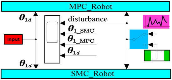
Figure 2. Block diagram of MPC and SMC comparison scheme.

Effective control of single-leg motion can be achieved by judicious selection of a suitable sliding-mode function. However, the switching gains required to address modeling uncertainties in SMC may lead to issues of decreased precision. As discussed in Section 4.1.1 and Section 4.1.2, when using a high gain (see Table 2), SMC outperformed the designed linear MPC in the displacement-tracking effect, while there were still high errors in contact-force tracking (refer to Figures 6–8 in Section 5.1). The LADRC, characterized by solid disturbance rejection capabilities and high control accuracy, represents an advanced control method. Consequently, in the subsequent section, we design the LADRC based on the SMC scheme to enhance the contact-force tracking effectiveness of the SMC scheme.

4.2. Design of Active Disturbance Rejection Controller

The fundamental principle of the LADRC involves leveraging the extended-state observer (ESO) to estimate diverse system states and internal and external disturbances [31]. When designing the LADRC, only the order of the controlled system and the control input gain are utilized, rendering the LADRC independent of the precise model of the controlled object. The order of the system changes depends on whether system delay is considered. Therefore, we first design an N-order LADRC controller.

4.2.1. N-Order Active Disturbance Rejection Control

Combining the expressions for our research subject in Equations (3), (5) and (20), a disturbed N-order system and an extended-state variable can be represented as:

$$\{\begin{array}{c}{z}^{\left(n\right)}=\Gamma \left(t,z\left(t\right),\dot{z}\left(t\right),\dots ,z^{\left(n-1\right)}\left(t\right)\right)+b_{0}u\\ \{\begin{array}{l}{\theta }_1=z,{\theta }_2=\dot{z},\dots ,{\theta }_n=z^{(n-1)}\hfill \\ {\theta }_{n+1}=\Gamma \left(t,z\left(t\right),\dot{z}\left(t\right),\dots ,z^{(n-1)}\left(t\right)\right)\hfill \end{array}\end{array},$$

(23)

where, $u,$ $b_0$, and $z\left(t\right)$ are the control input, coefficient, and output, respectively, of the N-order disturbed system, respectively. The $\Gamma$ denotes differentiable total disturbance. The ${\theta }_{n+1}$ is an extended-state variable. The linear ESO equation in the state-space form (Equation (24)) can be obtained by the state reconstruction of the linear extended-state observer using Equation (23), where ${\theta }_i$ is the actual value of the state variable. The observer’s estimated value is ${\widehat{\theta }}_i$. The gain matrix of the observer is $E$. Incorporating the transformation $\tilde{z}=\tilde{\theta }=\theta -\widehat{\theta }=z-\widehat{z}$, we can derive the error equation for the LESO. The error equation establishes that the LESO operates within a bounded input and output framework, and that the upper limit of the error is adjustable via ${\beta }_{{\omega }_o}\left(i\right)$. By judiciously selecting the appropriate values for $E$, the observer’s estimated value ${\widehat{\theta }}_i$ approximates the actual value of the state variable${\theta }_i$, where ${\theta }_i\approx {\widehat{\theta }}_i$:

$$\{\begin{array}{c}\dot{\hat{\theta }}=\dot{\hat{z}}=A\hat{\theta }+Bu+E(z-\hat{z})\\ \{\begin{array}{c}A=\left(\begin{array}{ccccc}0& 1& \dots & 0& 0\\ 0& 0& 1& \dots & 0\\ \dots & \dots & \dots & \dots & \dots \\ 0& 0& 0& 0& 0\end{array}\right),B=\left(\begin{array}{c}0\\ \dots \\ b_0\\ 0\end{array}\right),A\in R^{(n+1)\times (n+1)}\\ E=(\begin{array}{ccc}{\beta }_{{\omega }_o}(1)& {\beta }_{{\omega }_o}(2)\dots & { {\beta }_{{\omega }_o}(n) {\beta }_{{\omega }_o}(n+1))}^T\end{array}\end{array}\end{array},$$

(24)

To determine the expanded observer gain coefficient${ \beta }_{{\omega }_o}\left(i\right)$, we set the poles of the characteristics in Equation (25) (derived from Equation (24)) in the left-half plane. This method can reduce the adjustment parameters to bandwidth ${\omega }_o$ of the LESO. By modulating the observer’s bandwidth, we gain the flexibility to alter the overshooting behavior of the system:

$$\{\begin{array}{l}{L}_{LESO}\left(s\right)=s^{n+1}+{\beta }_{{\omega }_o}\left(1\right)s^n+{\beta }_{{\omega }_o}\left(2\right)s^{n-1}+\dots +{\beta }_{{\omega }_o}\left(n-1\right)={\left(s+{\omega }_o\right)}^{n+1}\hfill \\ {\beta }_{{\omega }_o}\left(i\right)=C_{n+1}^i{\omega }_o^i (i=1,2,3\dots ,n+1)\hfill \end{array},$$

(25)

Similarly, the controller’s bandwidth${ \omega }_c$ and the coefficients are expressed as follows:

$$\{\begin{array}{l}{s}^n+{\beta }_{{\omega }_c}\left(n\right)s^{(n-1)}+\dots +{\beta }_{{\omega }_c}\left(2\right)s+{\beta }_{{\omega }_c}\left(1\right)s^0={\left(s+{\omega }_c\right)}^n=0\hfill \\ {\beta }_{{\omega }_c}\left(i\right)=C_n^{n+1-i}{\omega }_c^{n+1-i} (i=2,3\dots ,n+1)\hfill \end{array},$$

(26)

The linear control law (Equation (27)) can be calculated using Equation (26):

$$u_{LADRC}=-\frac{1}{b_0}\cdot \left({\beta }_{{\omega }_c}(1)\left({\widehat{\theta }}_1-{\theta }_{1d}\right)+{\displaystyle \sum _{i=2}^{n+1}{\beta }_{{\omega }_c}}(i){\widehat{\theta }}_i\right),$$

(27)

According to the above theory, adjusting the observer and controller bandwidths allows us to modify the overshooting behavior of the system. We modeled the LADRC controller of the N-order system and designed a linear control law based on this. The stability of the LADRC is demonstrated; however, the required mathematical knowledge may be challenging for the reader, and References [32,33] is recommended.

Based on the above theoretical derivations and considerations, the LADRC operates independently of the precise models. Its control effectiveness depends on the system order, observer bandwidth, controller bandwidth, control coefficients, and initial state of the ESO. During the actual parameter-tuning process, we begin by establishing the order of the system and then determine the constant values for ${\omega }_o$ and ${\omega }_c$. Subsequently, we fine-tuned the $b_0$ and the initial values of the extended-state controller and adjusted them on a magnitude scale until the system output was aligned with the desired state.

4.2.2. Sliding Mode Control Comparison Group with and without Second-Order Linear Active Disturbance Rejection Loop

According to the comparative results of the control strategies in Section 4.1 and Section 4.2 (refer to Section 5.1), we cascaded the LADRC with an SMC to form a novel scheme (see Figure 3). By combining Equations (18), (20) and (27), the LADRC-SMC is shown in Figure 3.

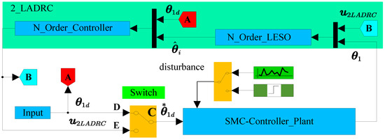
Figure 3. Switching schematic diagram of SMC comparison scheme with or without second-order LADRC loop.

Figure 3. Switching schematic diagram of SMC comparison scheme with or without second-order LADRC loop.

Equation (28) elucidates the transition mechanism on the second set of comparative strategies—namely, the SMC scheme and the LADRC-SMC scheme—as depicted in Figure 3. It is imperative to underscore that Figure 3 does not serve as a conventional control block diagram but rather as an illustrative representation of the transition process between contrasting methodologies. The engagement of the switching mechanism with CD signifies the execution of the SMC scheme. In Figure 3, C, D and E are the contact points of the switch respectively. ${\stackrel{*}{\theta }}_{1d}$ represents the optional input to the SMC control loop in the switching scheme. In comparison, its connection to CE denotes implementing the LADRC-SMC scheme. The signal $u_{2LADRC}$ from the LADRC loop is the input signal of the SMC loop in the LADRC-SMC scheme. The output signal ${\theta }_1$ of the SMC loop is the input signal of LESO in the LADRC loop. ${\widehat{\theta }}_i$ is the estimated value of the LESO in the LADRC loop, and ${\theta }_{1d}$ is the reference input of the two schemes:

$${\stackrel{*}{\theta }}_{1d}=\{\begin{array}{l}{\theta }_{1d}, \mathrm{Switch} \mathrm{to} \mathit{CD}\hfill \\ u_{2LADRC}=-\frac{1}{b_0}\cdot \left({\beta }_{{\omega }_c}(1)\left({\widehat{\theta }}_1-{\theta }_{1d}\right)+{\displaystyle \sum _{i=2}^3{\beta }_{{\omega }_c}}(i){\widehat{\theta }}_i\right), \mathrm{Switch} \mathrm{to} \mathit{CE}\hfill \end{array},$$

(28)

where ${\stackrel{*}{\theta }}_{1d}$ denotes the reference input for the SMC control loop. Switching to CD, which represents the SMC scheme, then ${\stackrel{*}{\theta }}_{1d}$ equals ${\theta }_{1d}$. Switching to CE, representing the LADRC-SMC scheme, then ${\stackrel{*}{\theta }}_{1d}$ equals $u_{2LADRC}$. System delay was not considered here. Based on the robotic single-leg dynamic model (Equation (5)), we set order N of the LADRC to 2. This configuration allows for the optimal utilization of their respective advantages, further enhancing system performance and stability. Notably, it addressed the challenge in SMC related to the weak tracking of the single-leg foot-end contact force of the robot (refer to Figure 10 and Figure 11 in Section 5.2).

4.2.3. Fourth-Order LADRC-SMC Comparison Group with or without SP Loop

Delays, including control and sensor delays, are inevitable in the design of robotic controllers. When the sensor delays are significant, they can potentially lead to controller instability (as shown in Figure 12 and Figure 14 in Section 5.3). If we define the total system delay as $D$, control delay as $D^{\mathrm{c}}$, and sensor delay as $D^{\mathrm{s}}$, then $D=D^{\mathrm{c}}+D^{\mathrm{s}}$. However, increasing this assumed delay did not yield satisfactory results after addressing the tracking issues of the joint angles and contact forces under disturbances using the previously designed LADRC-SMC. There are various approaches to address this issue, and we choose a simple and classical solution, SP [34,35], which forms a multi-loop control strategy (see Figure 4). This strategy decomposes the single-leg control system of a robot into multiple independent control loops, each of which is responsible for controlling specific variables or subsystems within the system. Finally, mathematical simulations verified that this strategy could enhance the system’s control performance, stability, and robustness. It allows for flexible adaptation to system variations and faults, improving control effectiveness (as shown in Figures 12–16 in Section 5.3).

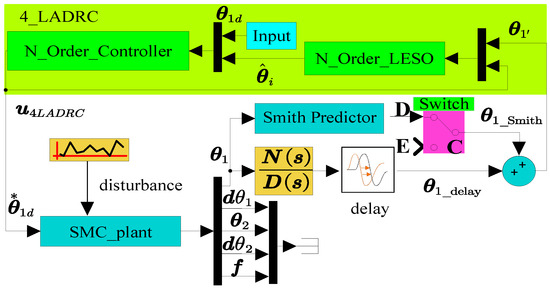
Figure 4. Switching diagram of fourth-order LADRC-SMC comparison scheme with or without SP loop.

Figure 4. Switching diagram of fourth-order LADRC-SMC comparison scheme with or without SP loop.

It is imperative to emphasize that Figure 4 is not a conventional control block diagram but an illustrative representation of the transition process between contrasting methodologies. In Figure 4, C, D and E are the contact points of the switch respectively. ${\stackrel{*}{\theta }}_{1d}$ represents the optional input to the SMC control loop in the switching scheme. In the presence of interference and delay, the engagement of the switching mechanism with CD signifies the execution of the LADRC-SMC-SP scheme. In comparison, its connection to CE denotes the implementation of the LADRC-SMC scheme. Regarding Figure 4, the closed-loop transfer function $G\left(S\right)$ of the LADRC-SMC-SP scheme can be ascertained in accordance with the SP principle:

$$G(S)=\frac{H_{\mathrm{c}}(\mathrm{s})S(\mathrm{s}){\mathrm{e}}^{-D^C}}{1+H_{\mathrm{c}}(\mathrm{s})S^{\prime }(\mathrm{s})+H_{\mathrm{c}}(\mathrm{s})\left(S(\mathrm{s}){\mathrm{e}}^{-D^S}-S^{\prime }(\mathrm{s}){\mathrm{e}}^{-{D^{\prime }}^S}\right)},$$

(29)

Here, $H_{\mathrm{c}}\left(\mathrm{s}\right)$ represents the transfer function of the residual portion in the LADRC-SMC-SP scheme, which does not include the sensor, whereas $S\left(\mathrm{s}\right)$ represents the transfer function of the sensor in the signal feedback loop. $D^S$ is the actual delay of the sensor. Pressure sensors with second-order system dynamics were used for the robot joint-angle and contact-force control. In the presented theoretical and applied research presented, $S^{\prime }\left(\mathrm{s}\right){\mathrm{e}}^{-D^{\prime S}}$ is the introduced predictive compensation transfer function. The sensor transfer function, denoted as $S\left(\mathrm{s}\right)$, represents a second-order system. When there is no model mismatch, we can get$S^{\prime }\left(\mathrm{s}\right)=S\left(\mathrm{s}\right),D^{\prime S}=D^S$. The $D^{\mathrm{c}}$ can be eliminated by controller design and parameter adjustment. $G\left(S\right)$in the LADRC-SMC-SP can be simplified as follows:

$$\{\begin{array}{l}G\left(S\right)=H_{\mathrm{c}}\left(\mathrm{s}\right)S\left(\mathrm{s}\right)/\left(1+H_{\mathrm{c}}\left(\mathrm{s}\right)S\left(\mathrm{s}\right)\right)\hfill \\ S\left(\mathrm{s}\right)=N\left(s\right)/D\left(s\right)=c_1/\left(c_2{s}^2+c_{3}s+c_4\right)\hfill \end{array},$$

(30)

where the parameters ${\displaystyle \sum _{i=1}^4}{c}_i=\left[5,1,3,5\right] (\mathrm{g}\mathrm{i}\mathrm{v}\mathrm{e}\mathrm{n} \mathrm{r}\mathrm{a}\mathrm{n}\mathrm{d}\mathrm{o}\mathrm{m}\mathrm{l}\mathrm{y}, \mathrm{w}\mathrm{i}\mathrm{t}\mathrm{h} \mathrm{s}\mathrm{u}\mathrm{b}\mathrm{s}\mathrm{t}\mathrm{i}\mathrm{t}\mathrm{u}\mathrm{t}\mathrm{a}\mathrm{b}\mathrm{i}\mathrm{l}\mathrm{i}\mathrm{t}\mathrm{y})$ are the coefficients of the sensor transfer function. In Equation (30), the closed-loop system does not include a lag term, and the lag component does not affect the characteristic equation of the system. Compared to systems without the SP, the system compensated by the SP eliminates the $D^{\mathrm{s}}$ during the control process. The control block diagram of LADRC-SMC-SP scheme finally proposed is shown in Figure 5.

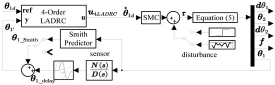
Figure 5. The control block diagram of the LADRC-SMC-SP scheme.

Figure 5. The control block diagram of the LADRC-SMC-SP scheme.

Equation (31) elucidates the transition mechanism on the third set of comparative strategies—namely, the LADRC-SMC and LADRC-SMC-SP schemes—as depicted in Figure 4. Signal $u_{4LADRC}$ from the LADRC loop is the input signal of the SMC loop in the LADRC-SMC and LADRC-SMC-SP schemes. The output signal ${\theta }_{1\prime }$ of the delay loop or predictor loop is the input signal of the LESO in the LADRC loop. ${\widehat{\theta }}_i$ is the estimated value of the LESO in the LADRC loop, and ${\theta }_{1d}$ is the reference input of the two schemes. The new switchable scheme (as shown in Figure 4) based on the LADRC-SMC scheme (as shown in Figure 3) is formed by combining Equations (18), (20), (27) and (31). This controller used the signal ($u_{4LADRC})$ from the LADRC loop as the reference input $\left({\stackrel{*}{\theta }}_{1d}\right)$ for the SMC loop. The signal ($u_{4LADRC})$ from the LADRC loop can be expressed using Equation (31):

$${\stackrel{*}{\theta }}_{1d}=u_{4LADRC}=\{\begin{array}{c}-\frac{1}{b_0}·({\beta }_{{\omega }_c}(1)({\hat{\theta }}_{1\mathrm{\_}\mathrm{Smith}}-{\theta }_{1d})+{\displaystyle \sum _{i=2}^5}{\beta }_{{\omega }_c}(i){\hat{\theta }}_{i\_\mathrm{Smith}}), \mathrm{Switch} \mathrm{to} CD\\ -\frac{1}{b_0}·({\beta }_{{\omega }_c}(1)({\hat{\theta }}_{1\mathrm{\_}\mathrm{delay}}-{\theta }_{1d})+{\displaystyle \sum _{i=2}^5}{\beta }_{{\omega }_c}(i){\hat{\theta }}_{i\mathrm{\_}\mathrm{delay}}), \mathrm{Switch} \mathrm{to} CE\end{array},$$

(31)

According to Equation (23), ${\widehat{\theta }}_{1\_\mathrm{S}\mathrm{m}\mathrm{i}\mathrm{t}\mathrm{h}}$ is the observed value of ${\theta }_{i\_\mathrm{S}\mathrm{m}\mathrm{i}\mathrm{t}\mathrm{h}}$ of the LADRC-SMC-SP scheme, and ${\widehat{\theta }}_{i\_\mathrm{S}\mathrm{m}\mathrm{i}\mathrm{t}\mathrm{h}}$ is the (i − 1) order derivative of the observed value of ${\widehat{\theta }}_{1\_\mathrm{S}\mathrm{m}\mathrm{i}\mathrm{t}\mathrm{h}}$ of the LADRC-SMC-SP scheme. ${\widehat{\theta }}_{1\_\mathrm{d}\mathrm{e}\mathrm{l}\mathrm{a}\mathrm{y}}$ is the observed value of ${\theta }_{i\_\mathrm{d}\mathrm{e}\mathrm{l}\mathrm{a}\mathrm{y}}$ in the LADRC-SMC scheme, and ${\widehat{\theta }}_{i\_\mathrm{d}\mathrm{e}\mathrm{l}\mathrm{a}\mathrm{y}}$ is the (i − 1) order derivative of the observed value of ${\widehat{\theta }}_{1\_\mathrm{d}\mathrm{e}\mathrm{l}\mathrm{a}\mathrm{y}}$ in the LADRC-SMC scheme. According to Equations (28) and (30), the system order of the LADRC-SMC-SP scheme is equivalent to the Fourth order. This multi-loop control strategy optimizes each control loop, thereby enhancing the system’s performance and stability. It is worth noting that the LADRC-SMC-SP scheme expands the solution to the sensor delay problem of the second-order LADRC-SMC single leg. The LADRC-SMC-SP scheme also realizes the challenges of weak single-foot contact-force tracking, oscillation problems in joint-angle tracking, and delay elimination (as shown in Figures 12–16 in Section 5.3). According to Equations (4), (18) and (19), the SMC loop law shown in Figure 4 (joint torque) can be reformulated, as shown in Equation (32):

$$\tau =\left\{\begin{array}{cc}{\tau }_{i\_\mathrm{Smith}}=\hfill & M_1\left({\theta }_{1\_\mathrm{Smith}}\right){\ddot{\theta }}_{†1\_\mathrm{Smith}}+C_1\left({\theta }_{1\_\mathrm{Smith}},{\dot{\theta }}_{1\_\mathrm{Smith}}\right){\dot{\theta }}_{†1\_\mathrm{Smith}}+G_1\left({\theta }_{1\_\mathrm{Smith}}\right)\hfill \\ \hfill & +K_P{r}_{L1}+J_{\varphi }^T\left({\theta }_{1\_\mathrm{Smith}}\right)f_{†}\hfill \\ {\tau }_{i\_\mathrm{delay}}=\hfill & M_1\left({\theta }_{1\_\mathrm{delay}}\right){\ddot{\theta }}_{†1\_\mathrm{delay}}+C_1\left({\theta }_{1\_\mathrm{delay}},{\dot{\theta }}_{1\_}\right){\dot{\theta }}_{†1\_\mathrm{delay}}+G_1\left({\theta }_{1\_\mathrm{delay}}\right)\hfill \\ \hfill & +K_P{r}_{L1}+J_{\varphi }^T\left({\theta }_{1\_\mathrm{delay}}\right)f_{†}\hfill \end{array},i=1,2\right.,$$

(32)

where ${\tau }_{1\_\mathrm{d}\mathrm{e}\mathrm{l}\mathrm{a}\mathrm{y}}$ is the torque of joint 1 in the LADRC-SMC scheme.${\tau }_{2\_\mathrm{S}\mathrm{m}\mathrm{i}\mathrm{t}\mathrm{h}}$ is the torque of joint 2 in the LADRC-SMC-SP scheme (as shown in Figure 14 in Section 5.3). Therefore, this new scheme, which combines SMC, ADRC, and SP, significantly improves the controllability of the research subject in terms of the disturbance rejection, stability, and robustness. The LADRC-SMC-SP scheme addresses the joint-angle and contact-force tracking deficiencies in the MPC and SMC schemes discussed in this study. In addition, it successfully resolved the sensor delay encountered in the LADRC-SMC scheme.

An SMC was designed to compare the tracking performance of the joint angles, and a predictive model control was reconstructed based on the existing literature (refer to the control-law design in Section 4.1.1 and Section 4.1.2 and the simulation analysis in Figures 6–8 in Section 5.1). A LADRC-SMC scheme was devised to address the issue of contact-force tracking accuracy (refer to the control-law design in Section 4.1.2, Section 4.2.1 and Section 4.2.2 and the simulation analysis in Figures 9–11 in Section 5.2). Considering the time delay in practical systems, a LADRC-SMC-SP scheme was constructed (refer to the control-law design in Section 4.2.1, Section 4.2.2 and Section 4.2.3 and the simulation analysis in Figures 12–16 in Section 5.3). Through the design of the controllers and relevant theoretical derivations, we completed the theoretical part of the design and proof. In the subsequent analysis, a series of numerical simulations were conducted to systematically compare and validate the efficacy of the designed LADRC-SMC-SP in mitigating external disturbances and alleviating the impact of time delays on the system. Additionally, a simulation analysis further validates and enhances the theoretical design outcomes of the three distinct schemes elucidated in Section 4.

5. Numerical Simulation and Validation Analysis

The controlled object is given by Equation (3), taking the related parameters of the robot leg as $p={\left[\begin{array}{ccccc}2.35& 0.9& 1& 1.75& 1\end{array}\right]}^T$ (this parameter is determined via the computation outlined in Equation (23) and the tabulated data presented in Table 1), and the initial state of the controlled objects ${\theta }_1 \mathrm{a}\mathrm{n}\mathrm{d} {\dot{\theta }}_1$ are $\left[1.5,0\right]$. The position command is $\theta =0.5+0.8\mathrm{s}\mathrm{i}\mathrm{n}t$ (reference input), and the ideal contact force is $f=50c\mathrm{o}\mathrm{s}t$ (reference input). In this algorithm simulation, the disturbance input is a common step or uniform random number disturbance. In the simulation, the selected parameters were as follows.

In Table 2, the parameters of various controllers were selected based on the control target of this study, the controllers’ principles, and the tuning experience. The parameter indexed as 1 was obtained through the synthesis of Equation (17) and the exposition provided in Section 4.1.1 in tandem with the empirical controller configurations. The parameter indexed as 2 was derived from the integration of Equation (19), supplemented by the discussion in Section 4.1.2 along with the empirical controller settings. The parameter indexed as 3 was acquired using an amalgamation of Equations (25)–(27) and elucidation in Section 4.2.2, in conjunction with empirical controller adjustments. The parameter indexed as 4 was obtained using Equations (25)–(27), the discussion in Section 4.2.3, and empirical controller configurations.

Table 2. Set physical parameters based on actual conditions.

Index	Controller	Parameters
1.	MPC	$k_1=15.42,k_2=5.55,k_3=k_1$
2.	SMC	$K_p=\left[\begin{array}{cc}5& 0\\ 0& 2\end{array}\right],K_f=140,∆=0.3$
3.	LADR-SMC	$\left[N,{\omega }_0,{\omega }_c,b_0\right]=\left[2,15,21,1.04\right],LESO=\left[1.5,-6.5,-15\right];P{a}_{SMC}=\left[K_p,K_f,∆\right]=\left[\left[\begin{array}{cc}5& 0\\ 0& 2\end{array}\right],140,0.3\right]$
4.	LADR-SMC-SP	$\left[N,{\omega }_0,{\omega }_c,b_0\right]=\left[4,5,10,100\right],LESO=\left[\mathrm{0,0},1,\mathrm{1,1}\right];$ $P{a}_{SMC}=\left[\left[\begin{array}{cc}5& 0\\ 0& 2\end{array}\right],140,0.3\right];$ ${\displaystyle \sum _{i=1}^4}{c}_i=\left[5,1,3,5\right]$

Table 2. Set physical parameters based on actual conditions.

Index	Controller	Parameters
1.	MPC	$k_1=15.42,k_2=5.55,k_3=k_1$
2.	SMC	$K_p=\left[\begin{array}{cc}5& 0\\ 0& 2\end{array}\right],K_f=140,∆=0.3$
3.	LADR-SMC	$\left[N,{\omega }_0,{\omega }_c,b_0\right]=\left[2,15,21,1.04\right],LESO=\left[1.5,-6.5,-15\right];P{a}_{SMC}=\left[K_p,K_f,∆\right]=\left[\left[\begin{array}{cc}5& 0\\ 0& 2\end{array}\right],140,0.3\right]$
4.	LADR-SMC-SP	$\left[N,{\omega }_0,{\omega }_c,b_0\right]=\left[4,5,10,100\right],LESO=\left[\mathrm{0,0},1,\mathrm{1,1}\right];$ $P{a}_{SMC}=\left[\left[\begin{array}{cc}5& 0\\ 0& 2\end{array}\right],140,0.3\right];$ ${\displaystyle \sum _{i=1}^4}{c}_i=\left[5,1,3,5\right]$

Based on the theoretical derivation sequence of the controller described earlier, three sets of comparative simulations were conducted to validate the effectiveness of the LADRC-SMC-SP scheme effectiveness further. Table 2 lists the three sets of comparative simulations. The initial comparison considered schemes in indexes 1 and 2, the second focused on schemes in indexes 2 and 3, and the third addressed schemes in indexes 3 and 4. The performance of the control systems is evaluated through comparative analysis, error rates, and metrics such as ISE. In control engineering, the ISE is commonly employed to assess the performance of closed-loop control systems, reflecting the extent to which the outputs of the system deviate from the desired values over the entire period. A smaller ISE value indicates better control system performance [36].

5.1. Numerical Simulation and Comparative Optimization of MPC and SMC Schemes under the Step or Random Disturbances

To evaluate the control effectiveness of the multi-loop controller, we conducted the first set of comparative simulations to evaluate the control effectiveness of the MLC. The MPC was reconstructed based on the literature mentioned in the introduction, specifically for the research object of this study. The SMC scheme was designed to address this research problem and is supported by theoretical proof. Because ${\theta }_2$ can be represented by ${\theta }_1$ (see Equation (4)), the tracking results for ${\theta }_1$ are emphasized. Through an analysis of the ISE index, the joint-angle tracking performance under the unit step and random disturbance inputs are presented separately to assess the tracking performance of the joint angles (see Figure 6 and Figure 7) and contact forces (see Figure 8) between the two controllers. Subsequently, a controller demonstrating a superior joint-angle tracking performance was selected to evaluate its contact-force tracking performance in the presence of diverse disturbances. According to the contact-force tracking situation, the controller with a strong position tracking performance was optimized and improved through the second group of comparison schemes.

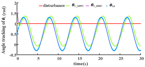
Figure 6. Joint-angle ${\theta }_1$ tracking of MPC and SMC schemes under unit step disturbance.

Figure 6. Joint-angle ${\theta }_1$ tracking of MPC and SMC schemes under unit step disturbance.

The positional command was given by $\theta =0.5+0.8\mathrm{s}\mathrm{i}\mathrm{n}t$. MPC and SMC are two widely employed, advanced robotic control strategies. A comparative analysis of the joint angle-tracking performance of these control schemes was conducted to discern their respective efficacies in the investigated scenarios. As illustrated in Figure 6, under identical unit step disturbance conditions, the tracking trends of joint angle ${\theta }_1$ are similar for both controllers. Nevertheless, the angle tracking of ${\theta }_{1\_\mathrm{M}\mathrm{P}\mathrm{C}}$ exhibits markedly inferior tracking performance regarding response speed, tracking amplitude, and synchronization compared to ${\theta }_{1\_\mathrm{S}\mathrm{M}\mathrm{C}}$. In Figure 6, the tracking trajectory of ${\theta }_{1\_\mathrm{S}\mathrm{M}\mathrm{C}}$ aligns with the reference signal trajectory${\theta }_{1d}$, deviating only within the initial 1 s interval. The relative merits of the SMC scheme are distinctly discernible based on the contrasting magnitudes of the ISE metric between the two schemes. Compared to the MPC scheme, the ISE for SMC at the angle ${\theta }_1$ is $1.1044\times 10^{-28} \mathrm{r}\mathrm{a}{\mathrm{d}}^2\cdot \mathrm{s}$ and $1.50147\times 10^{-2} \mathrm{r}\mathrm{a}{\mathrm{d}}^2\cdot \mathrm{s}$ for MPC, which indicates that the angle ${\theta }_1$ trajectory for SMC is more accurate than that for MPC. Consequently, SMC surpasses MPC in performance in unit step disturbance scenarios. Subsequently, we scrutinized the system performance under a uniform random disturbance (see Figure 7).

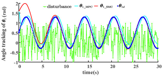
Figure 7. Joint-angle ${\theta }_1$ tracking of MPC and SMC schemes under uniform random disturbances.

Figure 7. Joint-angle ${\theta }_1$ tracking of MPC and SMC schemes under uniform random disturbances.

Figure 7 illustrates that under the same uniform random disturbance, the overall tracking trends of the joint angle ${\theta }_1$ for both controllers are similar. However, during the initial 0.5 s, the tracking trend of the MPC scheme opposes the reference trajectory, and only the SMC scheme comprehensively tracks the reference trajectory after 7.5 s. The angle ${\theta }_1$ trajectory for SMC is more accurate than that for MPC, as evidenced by the ISE values of $9.0265\times 10^{-29} \mathrm{r}\mathrm{a}{\mathrm{d}}^2\cdot \mathrm{s}$ for SMC and $0.0142464 \mathrm{r}\mathrm{a}{\mathrm{d}}^2\cdot \mathrm{s}$ for MPC. Because joint angle ${\theta }_2$ can be expressed in terms of joint angle ${\theta }_1$, the SMC also surpasses the MPC in the studied scenarios with a uniform random disturbance. Consequently, this study opts for an SMC scheme for further analysis and optimization by comparing these disturbances. Subsequently, we investigated the performance of the SMC scheme in tracking the contact force under these two disturbances (Figure 8).

The ideal contact force is represented by $f=50\mathrm{c}\mathrm{o}\mathrm{s}t$. In Figure 8, at time t = 22.3 s, the maximum tracking error of the contact force under unit step disturbance is 0.82167 $\mathrm{N}$. By calculation, the contact force at this time is 46.26048 $\mathrm{N}$, with an error peak ratio of 1.776%. At time $t=24.5 \mathrm{s}$, the maximum tracking error of the contact force under a uniform random disturbance was 8.34877 $\mathrm{N}$. By calculation, the contact force at this time was 45.49806 $\mathrm{N}$, and the error peak ratio was 18.350%. In the first group of winning SMC schemes, the ISE value of the contact-force tracking error under random disturbance is smaller than that under step disturbance, as evidenced by the ISE values of $2.2205\times 10^{-28} {\mathrm{N}}^2\cdot \mathrm{s}$ for random disturbance and $8.0582\times 10^{-30} {\mathrm{N}}^2\cdot \mathrm{s}$ for step disturbance. Consequently, the contact-force error of the SMC exhibits significant differences between the two types of disturbances.

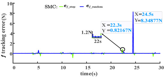
Figure 8. Comparison of ${\mathit{e}}_f$ of SMC schemes under two disturbances.

Figure 8. Comparison of ${\mathit{e}}_f$ of SMC schemes under two disturbances.

Figure 6, Figure 7 and Figure 8: In the first set of comparisons, the results indicate that while the SMC scheme outperforms the MPC scheme (compare References [13,14] in the introduction), there is room for improvement in reducing response time for joint-angle tracking and error rate for contact-force tracking under uniform random disturbance. To address this issue, we have combined the robust control capability of LADRC in suppressing external disturbances and model uncertainties with the ability of SMC to suppress parameter variations and unmodeled errors. The integration of LADRC and SMC enables each method to leverage its strengths, enhancing overall disturbance rejection performance and improving control effectiveness. For specific details and effects analysis, please refer to Equation (28) and Section 5.2 for comparative simulation results.

5.2. Simulation Verification and Comparative Analysis of LADRC-SMC and SMC Schemes under Uniform Random Disturbance

To implement the LADRC-SMC-SP scheme designed for the research problem, a comparative simulation of the second scheme was conducted based on the conclusions drawn from the comparative verification of the first scheme in Section 4.1, Section 4.2, and Section 5.1. A second-order LADR-SMC scheme is proposed in the theoretical section to improve the poor contact-force tracking performance of the SMC scheme. The joint angle tracking performance is shown in Figure 9.

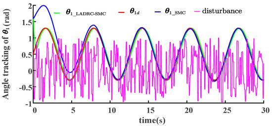
Figure 9. Joint angle ${\theta }_1$ tracking of LADRC-SMC and SMC schemes under uniform random disturbance.

Figure 9. Joint angle ${\theta }_1$ tracking of LADRC-SMC and SMC schemes under uniform random disturbance.

The joint-angle tracking performance, contact-force tracking ability (see Figure 10), and force tracking error (see Figure 11) in the second scheme were comprehensively analyzed by comparing the performances of the joint ${\theta }_1$ tracking and contact-force tracking under the influence of a uniform random disturbance. The effectiveness of the upgraded second-order LADR-SMC scheme was evaluated, and new challenges were discussed.

The position command is $\theta =0.5+0.8\mathrm{s}\mathrm{i}\mathrm{n}t$. To ensure the effective tracking of joint angle ${\theta }_1$, the two schemes were compared, and their corresponding joint-angle ${\theta }_1$ tracking results are presented in Figure 9. To ensure comparability of the second group of schemes, the values of the parameters $K_p,K_f,\mathrm{a}\mathrm{n}\mathrm{d} ∆$ in the LADRC-SMC scheme were consistent with those in the SMC scheme (refer to Table 2 in Section 5). Under the same uniform random disturbances, both controllers exhibited similar overall trends in tracking joint angle ${\theta }_1$. Regarding the response speed and convergence rate, the SMC scheme demonstrated significantly poorer tracking performance than LADRC-SMC. Although the tracking trend of the LADRC-SMC initially deviated from the reference trajectory for the first 0.5 s, it achieved comprehensive tracking of the reference trajectory around 1 s, while the SMC scheme only caught up with the reference trajectory after 7.5 s. Under the same uniform random disturbances, the angle ${\theta }_1$ trajectory for LADRC-SMC is more accurate than that for SMC, as evidenced by the ISE values of $7.4355\times 10^{-29} \mathrm{r}\mathrm{a}{\mathrm{d}}^2\cdot \mathrm{s}$ for LADRC-SMC and $9.0265\times 10^{-29} \mathrm{r}\mathrm{a}{\mathrm{d}}^2\cdot \mathrm{s}$ for SMC. By comparing the joint angle ${\theta }_1$ under these two disturbance scenarios, we can infer a similar situation for joint angle ${\theta }_2$, thus indicating the superiority of the LADRC-SMC method in joint-angle tracking. Next, we analyze the performance differences between the contact-force tracking schemes.

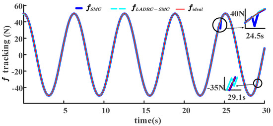
Figure 10. Contact-force tracking of LADRC-SMC and SMC schemes under random disturbance.

Figure 10. Contact-force tracking of LADRC-SMC and SMC schemes under random disturbance.

The ideal contact force is represented by $f=50\mathrm{c}\mathrm{o}\mathrm{s}t$. This study assumes that the contact force at the foot end of a lightweight-legged robot ranges from −50 $\mathrm{N}$ to 50 $\mathrm{N}$. The tracking of the contact and ideal contact forces is illustrated in Figure 10 for both schemes. Although both algorithms exhibit similar overall trends in tracking the ideal contact force, local fluctuations are observed. By zooming in on the highlighted fluctuation points in the figure, we can clearly observe the characteristics and trends of these fluctuations. Specifically, the LADRC-SMC algorithm exhibited the maximum fluctuation amplitude at time $t=24.5 \mathrm{s}$, whereas the SMC algorithm showed the maximum fluctuation amplitude at time $t=29.1 \mathrm{s}$. The specific differences are shown in Figure 11.

Under uniform random perturbations, Figure 11 shows that at $t=24.5 \mathrm{s}$, the maximum tracking error of the contact force for the SMC scheme was 8.34877 N. Thus, the contact force at this time was 45.49806 N, resulting in an error peak ratio of 18.350%. At $t=29.1 \mathrm{s}$, the LADRC-SMC scheme exhibited a maximum tracking error of 0.69991 N. The calculations indicate that the contact force was 43.68861 N, resulting in an error peak ratio of 1.602%. In the second comparison scheme, the contact-force tracking error ISE values were $2.2205\times 10^{-28} {\mathrm{N}}^2\cdot \mathrm{s}$ and $1.7293\times 10^{-29} {\mathrm{N}}^2\cdot \mathrm{s}$, close to 0. In Figure 9, the ISE metric of the LADRC-SMC scheme is also smaller than that of the SMC, indicating a higher control accuracy and a minor cumulative error for the LADRC-SMC scheme. Consequently, it can be concluded that the LADRC-SMC scheme addresses the high peak contact-force error rate observed in the winning SMC scheme of the first group, while ensuring the superiority of the ISE metric. Furthermore, under uniform random disturbances, the LADRC-SMC scheme reduces the peak contact-force error rate by more than tenfold while ensuring effective tracking of the joint angles.

Figure 11. Comparison of contact-force tracking error between LADRC-SMC and SMC schemes under random disturbance.

Figure 11. Comparison of contact-force tracking error between LADRC-SMC and SMC schemes under random disturbance.

Ensuring consistency between the parameters and interference conditions of the comparison scheme is a prerequisite for analyzing the comparison conclusion. The experimental results of the LADRC-SMC scheme demonstrate that innovative research combining different control methods is beneficial for exploring the advantages of their combination. The LADR-SMC ensures system stability, robustness, and disturbance rejection while achieving system tracking. Compared with the SMC, the LADR-SMC effectively addresses the issue of poor contact-force tracking under uniform random disturbances and guarantees joint-angle tracking (Compare References [16,19] in the introduction). However, performance degradation may occur in the LADR-SMC in practical scenarios owing to system delays. To investigate and address this issue, we conduct a simulation comparison of the third set of schemes in Section 5.3.

5.3. Simulation and Verification of LADR-SMC with Smith Predictor

To address the issue of poor tracking performance in the joint angle and contact force under interference delay, we developed a multi-loop control scheme called LADR-SMC-SP. This scheme is based on the LADR-SMC approach, demonstrating superior tracking performance discussed in Section 4.1.2, Section 4.2.2, and Section 5.2. We proposed a fourth-order LADR-SMC-SP scheme in the theoretical part of Section 4.2.3 to tackle the challenges related to force-position tracking and system delay. To further evaluate the effectiveness of the LADR-SMC-SP scheme, we conducted simulations to compare and discuss the tracking performance (see Figure 12 and Figure 13), joint torque (control law) (see Figure 14), force-tracking performance (see Figure 15 and Figure 16), and force-tracking errors of joints ${\theta }_1$ and ${\theta }_2$ under a uniform random disturbance. Subsequently, we evaluated the performance of the finalized multi-loop controller scheme and summarized its theoretical contributions to the application scenarios. In addition, we determined the significance and practical implications of the proposed scheme.

The position command was given by $\theta =0.5+0.8\mathrm{s}\mathrm{i}\mathrm{n}t$. Figure 12 shows the tracking results of the joint angle ${\theta }_1$ for the LADRC-SMC scheme with a uniform random disturbance and considering the system delay. To ensure the comparability of the three schemes, the parameters $K_p,K_f,\mathrm{a}\mathrm{n}\mathrm{d} ∆$ in the three schemes were consistent (refer to Table 2 in Section 5). ${\theta }_{1\_\mathrm{d}\mathrm{e}\mathrm{l}\mathrm{a}\mathrm{y}}$ represents the tracking result of the joint angle ${\theta }_1$ for the LADRC-SMC scheme without SP, whereas ${\theta }_{1\_\mathrm{S}\mathrm{m}\mathrm{i}\mathrm{t}\mathrm{h}}$ represents the tracking result of the joint angle ${\theta }_1$ for the LADRC-SMC-SP scheme. Ideal ${\theta }_{1d}$ represents the ideal tracking result of joint angle ${\theta }_1$. A system comparison with and without the predictor was performed using MATLAB/Simulink(Version information of simulation software: MATLAB R2023b) (Figure 4). The control delay was set to zero, and the sensor delay was set to 2 s.

The simulation results are shown in Figure 12. It can be observed that the control system without the Smith predictor (${\theta }_{1\_\mathrm{d}\mathrm{e}\mathrm{l}\mathrm{a}\mathrm{y}}$) exhibited a lag of 2 s and began to diverge after 10 s, whereas the control system with the Smith predictor (${\theta }_{1\_\mathrm{S}\mathrm{m}\mathrm{i}\mathrm{t}\mathrm{h}}$) exhibited a stable response, and the delay was effectively alleviated. The LADRC-SMC scheme diverges because the sensor time delay leads to a phase change in the feedback signal and a frequency response distortion (Equations (29) and (30) in Section 4.2.3). Under random disturbance and delay, the angle ${\theta }_1$ trajectory for LADRC-SMC-SP is more accurate than that for LADRC-SMC, as evidenced by the ISE values of $1.6636\times 10^{-28} \mathrm{r}\mathrm{a}{\mathrm{d}}^2\cdot \mathrm{s}$ for LADRC-SMC-SP and $2.4734\times 10^{-25} \mathrm{r}\mathrm{a}{\mathrm{d}}^2\cdot \mathrm{s}$ for LADRC-SMC. Therefore, the LADRC-SMC-SP scheme is superior to the LADRC-SMC scheme when considering the system delay under a uniform random disturbance.

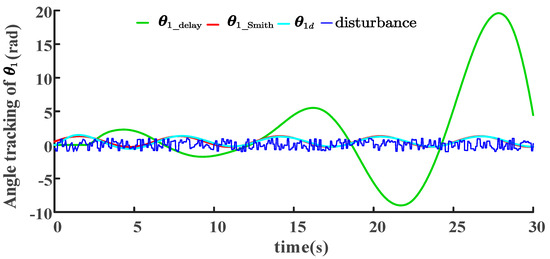
Figure 12. Tracking of joint angle ${\theta }_1$ in the LADRC-SMC scheme with or without the SP under random disturbance.

Figure 12. Tracking of joint angle ${\theta }_1$ in the LADRC-SMC scheme with or without the SP under random disturbance.

Next, we checked the tracking results for the joint angle ${\theta }_2$(see Figure 13). Because joint angle ${\theta }_2$ can be expressed in terms of joint angle ${\theta }_1$ (see Equation (4)), the tracking behavior of joint angle ${\theta }_2$ under the same conditions as those in Figure 11 is similar to that of joint angle ${\theta }_1$. Figure 13 shows the tracking results of the joint angle ${\theta }_2$ for the LADRC-SMC scheme with a uniform random disturbance and considering the system delay. ${\theta }_{2\_\mathrm{d}\mathrm{e}\mathrm{l}\mathrm{a}\mathrm{y}}$ represents the tracking result of the joint angle ${\theta }_2$ for the LADRC-SMC scheme without the SP, whereas ${\theta }_{2\_\mathrm{S}\mathrm{m}\mathrm{i}\mathrm{t}\mathrm{h}}$ represents the tracking result of the joint angle ${\theta }_2$ for the LADRC-SMC-SP scheme. The ideal $d{\theta }_{1d}$ represents the ideal tracking result of the joint angle ${\theta }_1$. Compared with the tracking behavior of joint angle ${\theta }_1$, the LADRC-SMC scheme without SP exhibits overall instability and irregular oscillations in the tracking of joint angle ${\theta }_2$. This phenomenon was more pronounced in the control law, as shown in Figure 14.

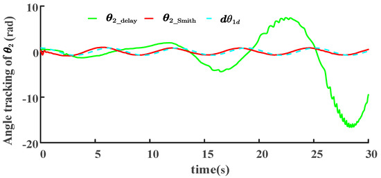
Figure 13. Tracking of joint angle ${\theta }_2$ in the LADRC-SMC scheme with or without the SP under random disturbance.

Figure 13. Tracking of joint angle ${\theta }_2$ in the LADRC-SMC scheme with or without the SP under random disturbance.

The LADRC-SMC-SP scheme shows the tracking behavior of joint angle ${\theta }_2$, which closely follows the trend of the ideal angle. Compared to LADRC-SMC, the ISE for LADRC-SMC-SP to the ${\theta }_{2\_\mathrm{S}\mathrm{m}\mathrm{i}\mathrm{t}\mathrm{h}}$ is $1.7983\times 10^{-28} \mathrm{r}\mathrm{a}{\mathrm{d}}^2\cdot \mathrm{s}$ and is $9.686\times 10^{-26} \mathrm{r}\mathrm{a}{\mathrm{d}}^2\cdot \mathrm{s}$ for LADRC-SMC to the ${\theta }_{2\_\mathrm{d}\mathrm{e}\mathrm{l}\mathrm{a}\mathrm{y}}$, which indicates that the ${\theta }_{2\_\mathrm{S}\mathrm{m}\mathrm{i}\mathrm{t}\mathrm{h}}$ trajectory for LADRC-SMC-SP is more accurate than LADRC-SMC. In conclusion, based on the tracking behavior of the joint angles in Figure 12 and Figure 13, it is evident that the LADRC-SMC-SP scheme outperforms the LADRC-SMC scheme under a uniform random disturbance and considers the system delay. Next, we examine the variation trajectory of the joint torque, that is, the change in the control parameter $\tau$ (see Figure 14), to further analyze the feasibility of the LADRC-SMC scheme with the SP.

Figure 14. Joint-torque tracking of LADRC-SMC scheme with or without SP under random disturbance.

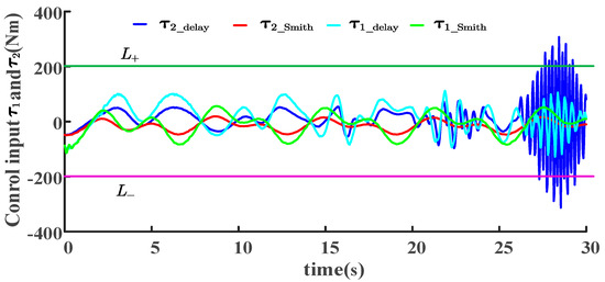
Figure 14. Joint-torque tracking of LADRC-SMC scheme with or without SP under random disturbance.

In this experiment, the position command was represented by the equation $\theta =0.5+0.8\mathrm{s}\mathrm{i}\mathrm{n}t$, whereas the ideal contact force was expressed as $f=50\mathrm{c}\mathrm{o}\mathrm{s}t$. Under the same experimental conditions as those shown in Figure 12 and Figure 13, the joint torque was simulated using the SMC law (Equation (32) in Section 4.2.3). In Figure 14, ${\tau }_{1\_\mathrm{d}\mathrm{e}\mathrm{l}\mathrm{a}\mathrm{y}}$ and ${\tau }_{2\_\mathrm{d}\mathrm{e}\mathrm{l}\mathrm{a}\mathrm{y}}$ illustrate the torque variation curves of joints 1 and 2, respectively, in the LADRC-SMC scheme. ${\tau }_{1\_\_\mathrm{S}\mathrm{m}\mathrm{i}\mathrm{t}\mathrm{h}}$ and${\tau }_{2\_\mathrm{S}\mathrm{m}\mathrm{i}\mathrm{t}\mathrm{h}}$ curves represent the torque variations of joints 1 and 2 in the LADRC-SMC-SP scheme. Notably, the lengths of the joints in the single-legged robot designed in this study were one meter each, which does not fall within the category of small-legged robots. Therefore, we take the example of an electric servo drive of a mechanical arm called “ABB IRB 6700-150/2.85: maximum torque of 285 $\mathrm{N}\cdot \mathrm{m}$.” This series of mechanical arms is equipped with different motor models, resulting in variations in their maximum torque. Considering factors related to the robot’s materials and structure, such as safety, stability, and reliability, we cautiously set the technical parameters of the joint drive motor in this study as follows: a saturation threshold torque of ±200 $\mathrm{N}\cdot \mathrm{m}$. The maximum output limit for the joint torque shown in Figure 14 is denoted as $L_{+}=200 \mathrm{N}\cdot \mathrm{m}$, whereas the minimum output limit is denoted as $L_{-}=-200 \mathrm{N}\cdot \mathrm{m}$.

After the analysis, we can draw the following conclusions: considering the system sensor delay, the fourth-order LADRC-SMC-SP scheme is more stable and reliable than the scheme without Smith’s compensation. The experimental results demonstrated that after 20 s of system operation, ${\tau }_{1\_\mathrm{d}\mathrm{e}\mathrm{l}\mathrm{a}\mathrm{y}}$ and ${\tau }_{2\_\mathrm{d}\mathrm{e}\mathrm{l}\mathrm{a}\mathrm{y}}$ in the control system without Smith compensation exhibited oscillatory instabilities. In particular, the ${\tau }_{2\_\mathrm{d}\mathrm{e}\mathrm{l}\mathrm{a}\mathrm{y}}$ exhibited oscillations at approximately 29 s and exceeded the servomotor saturation threshold of 200 $\mathrm{N}\cdot \mathrm{m}$. However, the joint torques in the control system with Smith compensation exhibited stable periodic variations without oscillations or exceeding the motor threshold. By considering the joint-angle tracking results in Figure 12 and Figure 13, as well as the joint-torque variations in Figure 14, it is evident that under uniform random disturbances and considering the system delay and motor threshold, the LADRC-SMC-SP scheme outperforms the scheme without the SP and demonstrates better feasibility. By compensating for the delay in advance, the LADR-SMC-SP mitigates the impact of the system delay on the control performance. The controller can accurately estimate and counteract system disturbances and improve the system’s robustness and control precision. In the next step, we will analyze the contact-force tracking results to validate the effectiveness of the LADRC-SMC-SP scheme.

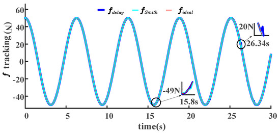
Figure 15. Contact-force tracking of LADRC-SMC scheme with or without SP under random disturbance.

Figure 15. Contact-force tracking of LADRC-SMC scheme with or without SP under random disturbance.

The ideal contact force is represented by $f=50\mathrm{c}\mathrm{o}\mathrm{s}t$. This study assumes that the contact force at the foot end of a lightweight-legged robot ranges from −50 $\mathrm{N}$ to 50 $\mathrm{N}$. The tracking of the contact force and ideal contact force is illustrated in Figure 15 for both schemes with and without SP. Although both algorithms exhibit similar overall trends in tracking the ideal contact force, local fluctuations are observed. By zooming in on the highlighted fluctuation points in the figure, we can clearly observe the characteristics and trends of these fluctuations. Specifically, the $f_{Smith}$ of the LADRC-SMC-SP scheme exhibited the maximum fluctuation amplitude at time $t=15.8 \mathrm{s}$, whereas the$f_{delay}$ of the LADRC-SMC scheme exhibited the maximum fluctuation amplitude at time $t=26.34 \mathrm{s}$. The specific differences are shown in Figure 16.

Figure 16. Comparison of contact-force tracking error of LADRC-SMC scheme with or without SP under random disturbance.

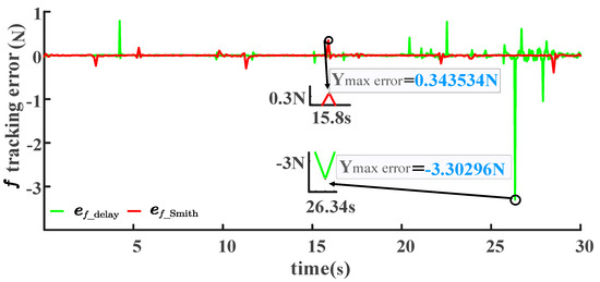
Figure 16. Comparison of contact-force tracking error of LADRC-SMC scheme with or without SP under random disturbance.

Under uniform random disturbances and considering the system delay, as shown in Figure 16, it can be observed that at t = 15.8 s, the maximum tracking error of the contact force for the LADRC-SMC-SP scheme is 0.343534 N. By calculation, the maximum contact force at this time is 48.11088996 N, resulting in an error rate of 0.687%. At t = 26.34 s, the maximum tracking error for the LADRC-SMC scheme is 3.30296 N. According to calculations, the top contact force at this time is 44.808845 N, resulting in an error rate of 7.371%. Figure 16 clearly illustrates that the LADRC-SMC-SP scheme significantly reduces the peak contact-force error rate by more than tenfold compared to the LADRC-SMC scheme. In the third comparison scheme, the ISE values of the contact-force tracking error are respectively $1.8062\times 10^{-30} {\mathrm{N}}^2\cdot \mathrm{s}$ and $4.6799\times 10^{-29} {\mathrm{N}}^2\cdot \mathrm{s}$, which are close to 0. In Figure 12 and Figure 13, the ISE metric of the LADRC-SMC-SP scheme is also smaller than that of the LADRC-SMC, indicating a higher control accuracy and more minor cumulative error for the LADRC-SMC-SP scheme. In conjunction with the analysis presented in Figure 12, Figure 13, Figure 14 and Figure 15, this finding demonstrates that the LADRC-SMC-SP scheme outperforms the LADRC-SMC scheme regarding joint angle, contact-force tracking, and control-law output amplitude.

The simulation results in Section 5.3 validate the superior performance of the LADRC-SMC-SP scheme compared to the LADRC-SMC scheme. This multi-loop controller aims to address the force-position tracking and system delay in legged robots under disturbances. The LADRC-SMC-SP system exhibited a stable response and effective delay suppression, whereas the LADRC-SMC system demonstrated instability and lag. The results of the analysis regarding the tracking behavior of joint angles ${\theta }_1$ and ${\theta }_2$ consistently support the superiority of the LADRC-SMC-SP scheme over the LADRC-SMC scheme. Analysis of the joint-torque variations revealed that the LADRC-SMC-SP scheme maintained stable periodic changes within the limits of the motor, whereas the LADRC-SMC scheme exhibited oscillatory instability and exceeded the motor saturation threshold. The tracking effectiveness of the contact force and the error analyses further validated the efficacy of the LADR-SMC-SP scheme. In conclusion, introducing SP in the LADR-SMC scheme enhances the control accuracy, improves system robustness, and is valuable for applying single-leg force-position tracking under interference delay and limited motor amplitude.

The LADRC-SMC-SP scheme effectively addresses the challenges associated with joint-angle and contact-force tracking control in a single-legged, multijoint robot. This LADRC-SMC-SP scheme overcomes the problems of disturbances, system delays, and motor limitations (Compare References [7,8,9] in the introduction). Through a comprehensive analysis of three different sets of controller designs and corresponding experimental simulations, the following conclusions can be drawn regarding our research topic:

• The LADRC-SMC-SP scheme improves the controller capabilities of each loop in a multi-loop system. LADRC addresses the challenges of external perturbations and model uncertainties in single-legged systems, SMC handles parameter variations and unmodelled errors, and SP resolves sensor delays. The multi-loop controller enhances the system’s robustness, stability, and convergence;
• The first set of comparison experiments demonstrated that the SMC scheme performed better in joint-angle tracking than the MPC scheme under step or uniform random interference. This implies that the robustness (Equations (18) and (19)), the response speed (Equations (17) and (19)), and the system structure (Equations (16) and (20)) of the designed SMC scheme are superior to those of the MPC scheme. However, the shortcomings of contact-force tracking also reveal the limitations and challenges of the SMC scheme, including the accuracy of contact-force modeling (Equations (8)–(10)), ability to handle nonlinear contact forces (refer to $f_{†}$ in Section 4.1.2), and the empirical nature of parameter adjustment (Table 2);
• The conclusion drawn from the second experiment is that the devised LADRC-SMC scheme not only guarantees accurate joint-angle tracking (see Equation (28) and Figure 9) but also significantly enhances the contact-force tracking performance (see Equations (25)–(27) and Figure 11). The LADRC-SMC scheme enhances the performance of single-legged systems by mitigating the two types of interference and achieving precise force-position tracking. Nevertheless, single-legged systems commonly encounter two types of delays (see Section 4.2.3), and the LADRC-SMC scheme is ineffective in addressing these delays (see Figure 12, Figure 13, Figure 14, Figure 15 and Figure 16);
• The findings of the third comparative experiment suggested that MPC, LADR-SMC, and LADR-SMC-SP exhibit progressive levels of optimality. The LADR-SMC-SP scheme effectively resolves multiple challenges in single-legged systems such as dual interference (refer to Figure 12, Figure 13, Figure 14, Figure 15 and Figure 16 and Equations (27) and (32)), dual delay (refer to Figure 12 and Figure 13 and Equations (29) and (30)), and motor limitations (Figure 14). In a single-legged system model, the LADR-SMC-SP scheme is well suited for contact-force control and position control of multijoint objects experiencing interference delay and limited motor amplitude;
• The design of this scheme has a strong portability. Regarding model design, the derivation of the reduced-order model is based on actual and reasonable physical scenarios. The derivation process is rigorous and can reflect the actual physical situation. In terms of parameter selection, the parameters in Table 1 were selected according to the physical knowledge and application scenarios with certain randomness. The parameters in Table 2 were manually adjusted according to the controller design theory and corresponding parameter design laws. The algorithm design and ISE index of the tracking error performance verify that the model design is reasonable and can adapt to various controllers. The LADRC-SMC-SP scheme stands out from the three groups of control schemes based on the literature in the introduction. Under the requirements of anti-interference, delay elimination, and motor saturation prevention in Section 5.1, Section 5.2 and Section 5.3, a better force-position tracking performance than other schemes is realized. This has a better effect on these problems than solutions in the literature [7,8,9] and creates a new reference for the control strategy of this type of model. In similar application scenarios, the scheme will have strong portability if the appropriate control parameters are selected according to the design principle of the scheme;
• There are limitations of theory and constraints of practice. The theory proposed in this paper is limited by tuning experience and does not employ intelligent parameter optimization methods. Therefore, this issue can be considered a direction for future research. Moreover, although the LADRC-SMC-SP scheme has strong portability, it is necessary to pay attention to various constraints during the foot-ground contact process of legged robots in practical applications. Therefore, the analysis of constraints is crucial to the design of control laws.

6. Conclusions

This study investigated the contact motion of a single-leg robot and proposed a series of improved control strategies, including MPC, SMC, LADRC-SMC, and LADRC-SMC-SP. This study aimed to explore the control performance of these strategies in a single-leg dynamic system, including disturbance rejection, measurement delay suppression, and avoidance of motor saturation. By comparing simulation experiments, the LADRC-SMC-SP strategy demonstrates the ability to simultaneously address the problems of disturbance delay and motor saturation, achieving satisfactory tracking control performance for joint angles and contact force. The main contributions of this study are as follows. First, a reduced-order dynamic model was successfully derived based on the model reduction theory and the parameter substitution method, which has the potential for various controller designs. Second, compared with existing theoretical and applied research, the LADRC-SMC-SP strategy combines the accurate position-tracking performance of the SMC strategy, the low contact-force tracking error of the LADRC-SMC strategy, and the ability to eliminate the oscillation divergence caused by the sensor delay of the SP strategy, effectively addressing the control challenges of the legged robot system. The contact-force peak error of the LADRC-SMC-SP scheme is ten times smaller than that of the LADRC-SMC scheme, which is far higher than that of other schemes. The ISE values for the tracking errors of joint angles ${\theta }_1$and ${\theta }_2$ and contact force $f$ are $1.6636\times 10^{-28} \mathrm{r}\mathrm{a}{\mathrm{d}}^2\cdot \mathrm{s}$, $1.7983\times 10^{-28} \mathrm{r}\mathrm{a}{\mathrm{d}}^2\cdot \mathrm{s}$, and $1.8062\times 10^{-30} {\mathrm{N}}^2\cdot \mathrm{s}$, respectively, which are close to 0, indicating excellent tracking control accuracy. Third, LADRC-SMC-SP overcomes the limitation of a single intelligent control method and provides a new idea for force-position control of legged robots. Finally, given the limitations of this study, a future optimization direction can be intelligent optimization of parameters to further expand the universality of the algorithm.

References

- Oral, D.Y.; Barkana, D.E.; Ugurlu, B. Centroidal momentum observer: Towards whole-body robust control of legged robots subject to uncertainties. In Proceedings of the 2022 IEEE 17th International Conference on Advanced Motion Control (AMC), Padova, Italy, 18–20 February 2022; pp. 432–437. [Google Scholar]
- Bhatti, J.; Hale, M.; Iravani, P.; Plummer, A.; Sahinkaya, N. Adaptive height controller for an agile hopping robot. Rob. Auton. Syst. 2017, 98, 126–134. [Google Scholar] [CrossRef]
- Li, X.; Feng, H.; Zhang, S.; Zhou, H.; Fan, Y.; Wang, Z.; Fu, Y. Vertical jump control of hydraulic single-legged robot (HSLR). In Proceedings of the 2019 IEEE/ASME International Conference on Advanced Intelligent Mechatronics (AIM), Hong Kong, China, 8–12 July 2019; pp. 1421–1427. [Google Scholar]
- Liu, C.; Zhang, T.; Liu, M.; Chen, Q. Active balance control of humanoid locomotion based on foot position compensation. J. Bionic. Eng. 2020, 17, 134–147. [Google Scholar] [CrossRef]
- Ren, H.; Zhang, L.; Su, C. Dynamic analysis and decoupled control of a heavy-duty walking robot with flexible feet based on super twisting algorithm. J. Meas. Control 2021, 54, 55–64. [Google Scholar] [CrossRef]
- Lu, Y.; Gao, J.; Shi, X.; Tian, D.; Liu, Y. Sliding balance control of a point-foot biped robot based on a dual-objective convergent equation. Appl. Sci. 2021, 11, 4016. [Google Scholar] [CrossRef]
- Alawad, N.A.; Humaidi, A.J.; Alaraji, A.S. Sliding Mode-Based Active Disturbance Rejection Control of Assistive Exoskeleton Device for Rehabilitation of Disabled Lower Limbs. An. Acad. Bras. Cienc. 2023, 95, e20220680. [Google Scholar] [CrossRef] [PubMed]
- Alawad, N.A.; Humaidi, A.J.; Alaraji, A.S. A novel approach of multi-loop control based-ADRC for improving lower knee position exoskeleton system. Int. Rev. Appl. Sci. Eng. 2023, 14, 316–324. [Google Scholar] [CrossRef]
- Alawad, N.A.; Humaidi, A.J.; Alaraji, A.S. Active disturbance rejection control with decoupling case for a lower limb exoskeleton of swing leg. ICIC Express Lett. 2023, 17, 1263–1275. [Google Scholar]
- Zhang, Z.; An, H.; Wei, X.; Ma, H. Unknown Slope-Oriented Research on Model Predictive Control for Quadruped Robot. Machines 2023, 11, 133. [Google Scholar] [CrossRef]
- Rybus, T.; Seweryn, K.; Sasiadek, J.Z. Control System for Free-Floating Space Manipulator Based on Nonlinear Model Predictive Control (NMPC). J. Intell. Robot. Syst. 2017, 85, 491–509. [Google Scholar] [CrossRef]
- Li, R.; Wang, H.; Yan, G.; Li, G.; Jian, L. Robust model predictive control for 2-DOF flexible-joint manipulator system. Mathematics 2023, 11, 3593. [Google Scholar] [CrossRef]
- Guechi, E.H.; Bouzoualegh, S.; Zennir, Y.; Blažič, S. MPC Control and LQ Optimal Control of A Two-Link Robot Arm: A Comparative Study. Machines 2018, 6, 37. [Google Scholar] [CrossRef]
- Tran, D.; Dao, H.V.; Ahn, K. Adaptive Synchronization Sliding Mode Control for an Uncertain Dual-Arm Robot with Unknown Control Direction. Appl. Sci. 2023, 13, 7423. [Google Scholar] [CrossRef]
- Zhang, Q.; Shen, D.; Tian, M.; Wang, X. Model-based Force Control of a Tendon-Sheath Actuated Slender Gripper Without Output Feedback. J. Intell. Robot. Syst. 2022, 106, 79. [Google Scholar] [CrossRef]
- Seul, J. Sliding Mode Control for a Hybrid Force Control Scheme of a Robot Manipulator Under Uncertain Dynamics. Int. J. Control Autom. Syst. 2023, 21, 1634–1643. [Google Scholar]
- Zhang, T.; Liang, X. Disturbance observer-based robot end constant contact force-tracking control. Complexity 2019, 2019, 5802453. [Google Scholar] [CrossRef]
- Pan, J.; Qu, L.; Peng, K. Fault-Tolerant Control of Multijoint Robot Based on Fractional-Order Sliding Mode. Appl. Sci. 2022, 12, 11908. [Google Scholar] [CrossRef]
- Liu, D.; Gao, Q.; Chen, Z.; Liu, Z. Linear Active Disturbance Rejection Control of a Two-Degrees-of-Freedom Manipulator. Math. Probl. Eng. 2020, 2020, 6969207. [Google Scholar] [CrossRef]
- Li, X.; Liu, B.; Wang, L. Control system of the six-axis serial manipulator based on active disturbance rejection control. Int. J. Adv. Robot. Syst. 2020, 17, 1–15. [Google Scholar] [CrossRef]
- Shi, X.; Huang, J.; Gao, F. Fractional-order active disturbance rejection controller for motion control of a novel 6-dof parallel robot. Math. Probl. Eng. 2020, 2020, 3657848. [Google Scholar] [CrossRef]
- Ramírez-Neria, M.; González-Sierra, J.; Luviano-Juárez, A.; Lozada-Castillo, N.; Madonski, R. Active Disturbance Rejection Strategy for Distance and Formation Angle Decentralized Control in Differential-Drive Mobile Robots. Mathematics 2022, 10, 3865. [Google Scholar] [CrossRef]
- Wang, H.D.; Li, X.; Liu, X.; Karkoub, M.; Zhou, L. Fuzzy sliding mode active disturbance rejection control of an autonomous underwater vehicle-manipulator system. J. Ocean Univ. China 2020, 19, 1081–1093. [Google Scholar] [CrossRef]
- Lu, K.; Tian, H.; Zhen, P.; Lu, S.; Chen, R. Conversion Flight Control for Tiltrotor Aircraft via Active Disturbance Rejection Control. Aerospace 2022, 9, 155. [Google Scholar] [CrossRef]
- Ji, P.; Min, F.; Ma, F.; Zhang, F.; Ni, D. Active Disturbance Rejection Terminal Sliding Mode Control for Tele-Aiming Robot System Using Multiple-Model Kalman Observers. Mathematics 2022, 10, 1268. [Google Scholar] [CrossRef]
- Zhang, D.; Wu, T.; Shi, S.; Dong, Z. A Modified Active-Disturbance-Rejection Control with Sliding Modes for an Uncertain System by Using a Novel Reaching Law. Electronics 2022, 11, 2392. [Google Scholar] [CrossRef]
- Duong, T.T.C.; Nguyen, C.C.; Tran, T.D. Synchronization Sliding Mode Control of Closed-Kinematic Chain Robot Manipulators with Time-Delay Estimation. Appl. Sci. 2022, 12, 5527. [Google Scholar] [CrossRef]
- Wu, Z.; Li, D.; Liu, Y.; Chen, Y. Performance Analysis of Improved ADRCs for a Class of High-Order Processes with Verification on Main Steam Pressure Control. IEEE Trans. Ind. Electron. 2023, 70, 6180–6190. [Google Scholar] [CrossRef]
- Su, C.Y.; Leung, T.P.; Zhou, Q.J. Force/motion control of constrained robots using sliding mode. IEEE. Trans. Autom. Control 1992, 37, 668–672. [Google Scholar] [CrossRef]
- Ohhira, T.; Shimada, A. Model Predictive Control for an Inverted-Pendulum Robot with Time-Varying Constraints. IFAC-PapersOnline 2017, 50, 776–781. [Google Scholar] [CrossRef]
- Han, J. Active Disturbance Rejection Control Technique—The Technique for Estimating and Compensating the Uncertainties; National Defense Industry Press: Beijing, China, 2008; Chapters 1–3. [Google Scholar]
- Wan, H.; Xiaohui, Q.I.; Jie, L.I. Stability analysis of linear/nonlinear switching active disturbance rejection control based MIMO continuous systems. J. Syst. Eng. Electron. 2021, 32, 956–970. [Google Scholar]
- Guo, B.Z.; Wu, Z.H. Output tracking for a class of nonlinear systems with mismatched uncertainties by active disturbance rejection control. Syst. Control Lett. 2017, 100, 21–31. [Google Scholar] [CrossRef]
- Baskys, A. Switched-Delay Smith Predictor for the Control of Plants with Response-Delay Asymmetry. Sensors 2023, 23, 258. [Google Scholar] [CrossRef] [PubMed]
- Wang, J.; Wu, G.; Sun, B.; Ma, F.; Aksun-Guvenc, B.; Guvenc, L. Disturbance Observer-Smith Predictor Compensation-Based Platoon Control with Estimation Deviation. J. Adv. Transp. 2022, 2022, 9866794. [Google Scholar] [CrossRef]
- Ayala-Olivares, J.R.; Enríquez-Caldera, R.; Guerrero-Castellanos, J.F.; Durand, S. Attitude Synchronization of Rigid Bodies with Event-Triggered Communication. IEEE Access 2023, 11, 88869–88880. [Google Scholar] [CrossRef]
Disclaimer/Publisher’s Note: The statements, opinions and data contained in all publications are solely those of the individual author(s) and contributor(s) and not of MDPI and/or the editor(s). MDPI and/or the editor(s) disclaim responsibility for any injury to people or property resulting from any ideas, methods, instructions or products referred to in the content. |
© 2024 by the authors. Licensee MDPI, Basel, Switzerland. This article is an open access article distributed under the terms and conditions of the Creative Commons Attribution (CC BY) license (https://creativecommons.org/licenses/by/4.0/).