Feature Optimization-Based Machine Learning Approach for Czech Land Cover Classification Using Sentinel-2 Images

Abstract

The Czech Republic is one of the countries along the Belt and Road Initiative, and classifying land cover in the Czech Republic helps to understand the distribution of its forest resources, laying the foundation for forestry cooperation between China and the Czech Republic. This study aims to develop a practical approach for land cover classification in the Czech Republic, with the goal of efficiently acquiring spatial distribution information regarding its forest resources. This approach is based on multi-level feature extraction and selection, integrated with advanced machine learning or deep learning models. To accomplish this goal, the study concentrated on two typical experimental regions in the Czech Republic and conducted a series of classification experiments, using Sentinel-2 and DEM data in 2018 as the main data sources. Initially, this study extracted various features, including spectral, vegetation, and terrain features, from the study area, then assessed and selected key features based on their importance. Additionally, this study also explored multi-level spatial contextual features to improve classification performance. The extracted features include texture and morphological features, as well as deep semantic information learned by utilizing a deep learning model, 3D CNN. Finally, an AdaBoost ensemble learning model with the random forest as the base classifier is designed to produce land cover classification maps, thus obtaining the spatial distribution of forest resources. The experimental results demonstrate that feature optimization significantly enhances the extraction of high-quality features of surface objects, thereby improving classification performance. Specifically, morphological and texture features can effectively enhance the discriminability between different features of surface objects, thereby improving classification accuracy. Utilizing deep learning networks enables more efficient extraction of deep feature information, further enhancing classification accuracy. Moreover, employing an ensemble learning model effectively boosts the accuracy of the original classification results from different individual classifiers. Ultimately, the classification accuracy of the two experimental areas reaches 92.84% and 93.83%, respectively. The user accuracies for forests are 92.24% and 93.14%, while the producer accuracies are 97.71% and 97.02%. This study applies the proposed approach for nationwide classification in the Czech Republic, resulting in an overall classification accuracy of 90.98%, with forest user accuracy at 91.97% and producer accuracy at 96.2%. The results in this study demonstrate the feasibility of combining feature optimization with the 3D Convolutional Neural Network (3DCNN) model for land cover classification. This study can serve as a reference for research methods in deep learning for land cover classification, utilizing optimized features.

1. Introduction

Forests play crucial roles in the economy, ecology, and society, exerting positive influences on the livelihoods of local residents, promoting sustainable economic growth, and mitigating climate change. Serving as habitats for diverse flora and fauna, forests provide essential environmental services, expanding their influence from rural and local economies to encompass social functions at both local and global levels [1]. Within the framework of the “17 + 1” (China-Central and Eastern European Countries Cooperation), forestry cooperation carries undeniable importance. Recognizing the critical role of forests from the onset, China and Central and Eastern European countries have forged partnerships among commercial and research entities, with government support, to enhance forestry cooperation. Located along the Belt and Road Initiative, the Czech Republic (hereinafter referred to as Czech) possesses abundant forest resources. This collaborative endeavor between China and Czech promotes economic prosperity, ecological balance, and social sustainability, making substantial contributions to the sustainable advancement of forestry for both nations [2]. Hence, it is crucial to acquire the spatial distribution of forest resources in Czech. Traditional field-based forest surveys are costly, inefficient, labor-intensive, and time-consuming, posing challenges in meeting the needs for large-scale forest resource assessments. Conversely, remote sensing technology offers substantial advantages in acquiring forest resources, including extensive monitoring coverage, cost-effectiveness, and timely data availability, demonstrating significant potential [3,4,5]. Therefore, the utilization of remote sensing image classification methods to obtain land cover classification results can facilitate the acquisition of spatial distribution information for forest resources.

Traditional remote sensing image classification methods are generally classified into two types: Pixel-based classification and object-oriented classification. In pixel-based classification methods, Foody et al. [6] utilized artificial neural networks to classify Brazilian tropical forests, demonstrating superior performance compared to traditional approaches. Zhang et al. [7] classified forest types into four categories—broadleaf forests, coniferous forests, mixed forests, and other land uses—using dynamic clustering and combined supervised classification methods. The study concluded that the combined supervised classification method achieved higher classification accuracy. In object-oriented classification methods, Mao et al. [8] conducted land cover classification in the Qianjiangyuan National Park using Sentinel-2 and Sentinel-1 data, comparing pixel-based and object-oriented approaches. They found that the object-oriented method produced superior classification results. Similarly, Tan et al. [9] compared pixel-based and object-based methods for urban vegetation classification, with results indicating the superiority of object-oriented classification. The above studies demonstrate that, compared to pixel-based methods, object-oriented approaches offer advantages in classifying images by clustering individual pixels based on spectral characteristics into textured geospatial objects. This approach effectively mitigates the occurrence of “salt and pepper” noise in classification results and enhances better overall coherence.

The key to land cover classification lies in feature extraction and classification methods. Feature selection and extraction are critical factors influencing the accuracy of land cover classification [10]. However, existing studies exhibit some limitations in feature selection. Firstly, traditional land cover classification features mainly depend on spectral information, which is sensitive to factors such as illumination and seasonal changes [11], thus constraining classification accuracy. Secondly, individual features struggle to fully capture the complexity and diversity of land cover types [12], thus reducing classifier performance. Additionally, researchers frequently neglect the interactions among features of surface objects and nonlinear relationships during the process of feature extraction [13], leading to limitations in the classification outcomes. To enhance the accuracy of land cover classification further, researchers have started to concentrate on methods that incorporate the fusion of multi-source data and combinations of multiple features to address the limitations of individual features in classification [14].

In the domain of deep learning classification, He et al. [15] proposed a multi-scale 3D convolutional neural network model. This model intelligently combines spectral and spatial features extracted from remote sensing images in an end-to-end manner, thereby improving classification accuracy. To mitigate computational costs, Liu et al. proposed a preprocessing-free classification model based on 3D convolutional neural networks (3DCNN), which directly input hyperspectral images into the 3DCNN [16]. Palsson et al. [17] decreased the band dimension of HRSI before using 3DCNN to extract features. However, this approach led to the loss of spectral continuity in image data, affecting classification accuracy. Mei et al. [18] and Sellami et al. [19] classified the spectral-spatial features obtained from the 3DCNN model. Roy et al. [20] also combined 3DCNN with 2DCNN, where 3DCNN first extracted spectral-spatial features, followed by refinement by 2DCNN [21].

Recently, the field of remote sensing classification has widely embraced ensemble classification methods. Xia et al. [22] developed five random forest ensemble models, including bagging-based, boosting-based, random subspace (RS)-based, rotation-based, and boosted-based approaches. These approaches effectively enhanced the prediction accuracy of the random forest ensemble system. Chen et al. [23] utilized convolutional neural networks (CNNs) and deep residual networks (ResNets) as base classifiers, advancing the development of ensemble learning through a deep learning-based random subspace ensemble framework. Chi et al. [24] have achieved excellent recognition performance by combining multiple collaborative representations with boosting techniques.

This study focuses on two typical regions in Czech, namely the South and East. It aims to address the shortcomings in feature selection methods in current land cover classification approaches for Czech, resulting in poor classification accuracy and effectiveness. We propose the utilization of 3DCNN deep learning networks for feature extraction and ensemble learning methods for land cover classification to address the challenge of acquiring spatial distribution data for forest resources. The research data consist of Sentinel-2 satellite images and DEM data, which are utilized for extracting features, including spectral, vegetation, and terrain features. Calculations for texture and morphological features are planned to enhance the utilization of spectral information in images. Additionally, the use of 3DCNN networks for extracting deep semantic information from images enables more effective differentiation of various land cover categories. Finally, these features are input into ensemble learning classifiers to investigate classification performance. This study can serve as a reference for research methods in deep learning for land cover classification, utilizing optimized features.

The main contributions and innovations of this study are as follows:

(1)

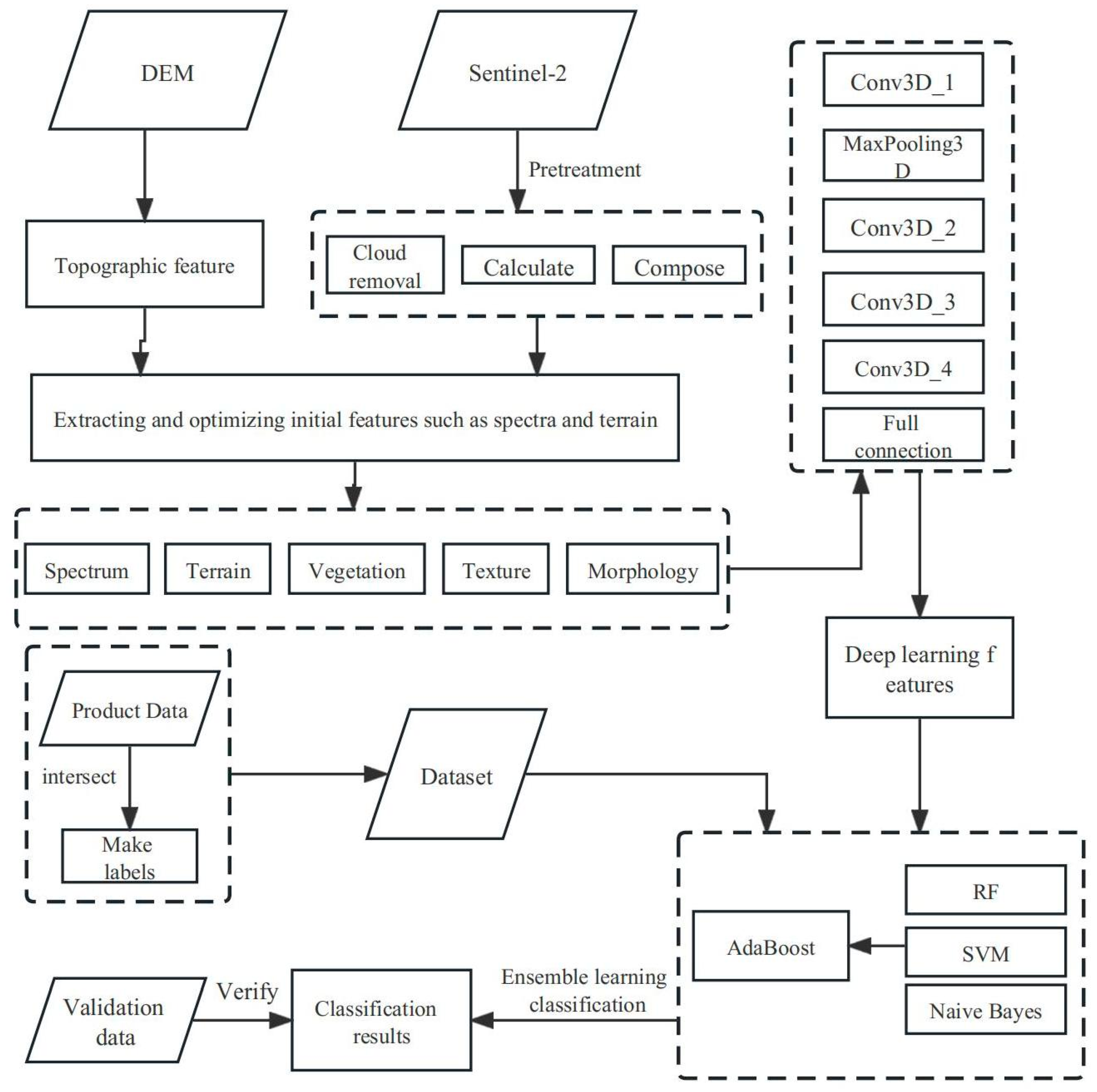
This study explores the importance of feature engineering and optimization in Czech land cover classification. Initially, this study extracts multidimensional features from remote sensing images of the experimental area, encompassing spectral, texture, morphological, and topographical features. The importance of the extracted features is compared experimentally to make the final optimization. Subsequently, a 3DCNN model is applied to explore the deep-level semantic features of land objects based on the selected features, thereby improving the differences of different land categories in the imagery.

(2)

This study proposes a feature optimization-based machine learning approach for Czech land cover classification, achieving promising results. It offers insights into the application of deep learning methods in land classification research, particularly with regard to feature selection.

(3)

This study’s findings demonstrate significant improvements in land cover classification through the utilization of multiple features and feature optimization. Furthermore, the utilization of deep neural network models enhances feature extraction capabilities, while ensemble classification methods improve classification results to some extent.

2. Materials and Methods

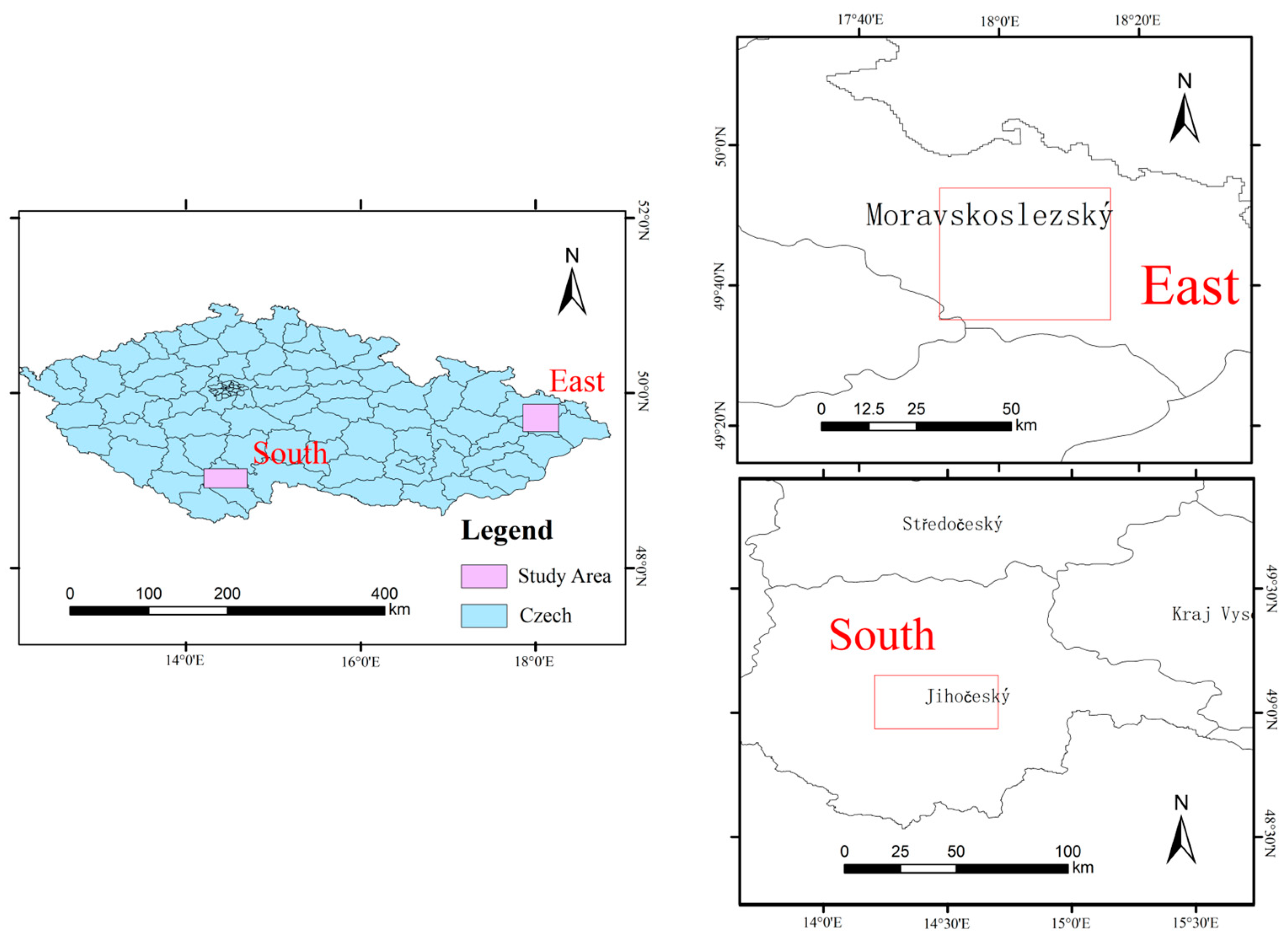
2.1. Study Area

Czech, situated in Central Europe, covers an area of 127,900 square kilometers. The country has a temperate climate characterized by hot summers and cold winters, often accompanied by substantial snowfall. July is typically the warmest month, whereas January is the coldest. The continental climate becomes more pronounced from west to east. Annual precipitation ranges between 600 and 800 mm, with certain mountainous regions receiving up to 1500 mm of rainfall. The terrain of Czech is diverse, with the western half comprising basins, hills, and plateaus, bordered by mountain ranges such as the Sudetes, Krkonoše, and Šumava. The eastern part is primarily situated in the Western Carpathians, with around 35% of the land covered by forests, indicating plentiful forest resources.

This study selected two experimental areas, namely East and South areas, situated in Czech. Both areas cover all types of land cover, reflecting the overall distribution of land cover in Czech. Moreover, they represent a larger proportion of land cover types with minimal coverage compared to other areas. The spatial relationship between the experimental areas is depicted in Figure 1.

2.2. Data Collection and Processing

2.2.1. Image Data

The data utilized in this study consist of Sentinel-2 satellite imagery and DEM, all obtained from the GEE platform database. Specifically, nine spectral bands from Sentinel-2 imagery were chosen, with details provided in

Table 1. Sentinel-2 spectral band information.

Sentinel-2 Band	Center Wavelength (μm)	Resolution (m)
Band 2—Blu-ray	$0.4$90	10
Band 3—Green Light	0.560	10
Band 4—Red Light	0.665	10
Band 5—Red Edge 1	0.705	20
Band 6—Red Edge 2	0.740	20
Band 7—Red Edge 3	0.783	20
Band 8—Near Infrared	0.842	10
Band 8A—Narrow Wave NIR	0.865	20
Band 11—Shortwave Red 1	0.945	60
Band 12—Shortwave Red 2	1.375	60

. Using a cloud removal algorithm, images from 2018 were selected, ensuring cloud coverage did not exceed 10% in the chosen areas of Czech. These images underwent radiometric, geometric, and atmospheric corrections as part of preprocessing, which involved resampling, clipping, and mosaicking.

2.2.2. Sample Data

In this study, the training data were gathered from diverse sources, namely: (1) GlobeLand30 [25] (http://www.globallandcover.com (accessed on 17 May 2023)), offering global land cover data at a 30 m spatial resolution for the years 2000, 2010, and 2020. We specifically chose the 2020 version, developed by the National Geomatics Center of China. (2) GLC_FCS 30 [26] (https://doi.org/10.5281/zenodo.3551994 (accessed on 26 May 2023)), a global land cover classification product with a 30 m resolution, released by the Aerospace Information Research Institute of the Chinese Academy of Sciences. This dataset is updated every five years from 1985 to 2020, and we selected data from 2015 and 2020. (3) Pflugmacher et al. [27] recently devised an independent method for pan-European land cover mapping using Landsat data at a 30 m resolution for 2015 (https://doi.pangaea.de/10.1594/PANGAEA.896282 (accessed on 28 May 2023)). (4) The ECL10 product [28], crafted using multi-source Earth observation data, particularly focusing on the integration of Sentinel-1 and Sentinel-2 data, to generate a land cover map for 2020 (https://doi.org/10.5281/zenodo.4407051 (accessed on 19 May 2023)).

The land cover categories considered in this study encompass Cropland, Forest, Grass, Shrub, Wetland, Water, Impervious, with the data obtained from the intersection of the different datasets. The selected categories are all encompassed in the previously mentioned products, and their prevalence is notably high. A system transformation has been devised based on the distinctions among various products [27,29].

After obtaining various land use classification products, this study initially resampled the spatial resolution of each product to 10 m using interpolation. The interpolation method utilized was nearest neighbor interpolation, a straightforward technique that assigns the value of the target point to that of the nearest known point. Subsequently, the classification attributes of each product were transformed into uniform categories for this study through category merging and attribute editing. The modified products were intersected to create a composite raster dataset. Training point data were sampled from this dataset. Due to the scarcity of categories such as shrubland and bare land, the sample sizes were adjusted uniformly to the maximum available. Training points were randomly selected from two experimental areas, South and East, then divided into training and validation datasets in a 7:3 ratio. The distribution of training and validation data, along with detailed sample sizes, is depicted in Figure 2 and

Table 2. Sample size.

Land Category	East		South
	Number of Training Samples	Number of Validation Samples	Number of Training Samples	Number of Validation Samples
Cropland	682 (69.03%)	306 (30.92%)	874 (69.53%)	383 (30.47%)
Forest	576 (72.45%)	219 (27.55%)	401 (70.47%)	168 (29.53%)
Grass	24 (68.57%)	11 (31.34%)	41 (70.69%)	17 (29.31%)
Shrub	16 (80.00%)	4 (20.00%)	36 (80.00%)	9 (20.00%)
Wetland	7 (70.00%)	3 (30.00%)	7 (77.78%)	2 (22.22%)
Water	81 (65.85%)	42 (34.15%)	7 (63.64%)	4 (36.36%)
Impervious	46 (60.53%)	30 (39.47%)	223 (69.47%)	98 (30.53%)

. The numbers in parentheses indicate percentages. To input optimized feature variables for deep feature extraction into the convolutional neural network, a label dataset for deep learning was established. A 1-pixel * 1-pixel area centered on each selected sample point was designated as the label for deep learning.

2.3. Methods

This study utilizes the Google Earth Engine (GEE) platform to obtain Sentinel-2 imagery and digital elevation model (DEM) data, thereby generating a dataset of samples and labels through the intersection of processed product data. Initially, features were extracted from the Sentinel-2 images and DEM data, including spectral bands, vegetation index, and terrain factors. Subsequently, random forest was applied to evaluate feature importance for reducing data dimensionality and selecting high-quality features for classification. Following this, multi-level spatial features and deep semantic information were extracted to improve classification performance, incorporating texture and morphological features. During this process, a pre-constructed dataset of samples and labels was utilized to extract and integrate deep semantic features using a 3D convolutional neural network (3DCNN), resulting in high-quality features with strong discriminative power for subsequent land cover classification. Finally, a classification model was designed to accomplish the ultimate land cover classification, utilizing RF as the base classifier and employing the AdaBoost strategy in ensemble learning. The technical workflow of this study is depicted in Figure 3.

2.3.1. Initial Feature Extraction and Optimization

Initially, this study acquired spectral features and supplemented them with vegetation indices, terrain factors, and other variables to create a multispectral feature dataset. Subsequently, random forest was utilized to evaluate the importance of these features, and their importance was ranked accordingly. Finally, a new feature set was chosen based on the ranking results. The Sentinel-2 composite imagery comprises nine spectral bands, used to compute a series of vegetation indices. These indices include the Normalized Difference Vegetation Index (NDVI), Normalized Difference Water Index (NDWI), Bare Soil Index (BSI), Normalized Difference Tillage Index (NDTI), Soil Adjusted Vegetation Index (SAVI), and Normalized Difference Built-up Index (NDBI). The formulas for computing these indices are provided in

Table 3. Spectral index.

Index	Formula	References
NDVI	$\frac{\mathrm{N}\mathrm{I}\mathrm{R}-\mathrm{R}\mathrm{E}\mathrm{D}}{\mathrm{N}\mathrm{I}\mathrm{R}+\mathrm{R}\mathrm{E}\mathrm{D}}$	[30]
SAVI	$\frac{\mathrm{N}\mathrm{I}\mathrm{R}-\mathrm{R}\mathrm{E}\mathrm{D}}{(\mathrm{N}\mathrm{I}\mathrm{R}+\mathrm{R}\mathrm{E}\mathrm{D}+0.5)\times 1.5}$	[31]
NDWI	$\frac{\mathrm{G}\mathrm{R}\mathrm{E}\mathrm{E}\mathrm{N}-\mathrm{S}\mathrm{W}\mathrm{I}\mathrm{R}2}{\mathrm{G}\mathrm{R}\mathrm{E}\mathrm{E}\mathrm{N}+\mathrm{S}\mathrm{W}\mathrm{I}\mathrm{R}2}$	[32]
NDTI	$\frac{\mathrm{S}\mathrm{W}\mathrm{I}\mathrm{R}1-\mathrm{S}\mathrm{W}\mathrm{I}\mathrm{R}2}{\mathrm{S}\mathrm{W}\mathrm{I}\mathrm{R}1+\mathrm{S}\mathrm{W}\mathrm{I}\mathrm{R}2}$	[33]
BSI	((RED + SWIR1) $-$ (NIR + BLUE))/((RED + SWIR1) + (NIR + BLUE))	[34]
NDBI	(SWIR1 − NIR)/(SWIR + NIR)	[35]

. BLUE in the table represents blue band B2, GERRN represents green band B3, RED represents red band B4, NIR represents near-infrared band B8, SWIR1 represents shortwave infrared band B11, and SWIR2 represents shortwave infrared band B12.

Initially, this study acquired spectral features and supplemented them with vegetation indices, terrain factors, and other variables to create a multispectral feature dataset. Subsequently, random forest was utilized to evaluate the importance of these features, and their importance was ranked accordingly. Finally, a new feature set was chosen based on the ranking results. The Sentinel-2 composite imagery comprises nine spectral bands, used to compute a series of vegetation indices. The formulas for computing these indices are provided in Table 3.

The mean, maximum, and standard deviation of each index were computed as classification features after acquisition. Additionally, three terrain features, including slope, aspect, and elevation extracted from DEM data, were incorporated. A total of 17 spectral, vegetation index, and terrain features were obtained.

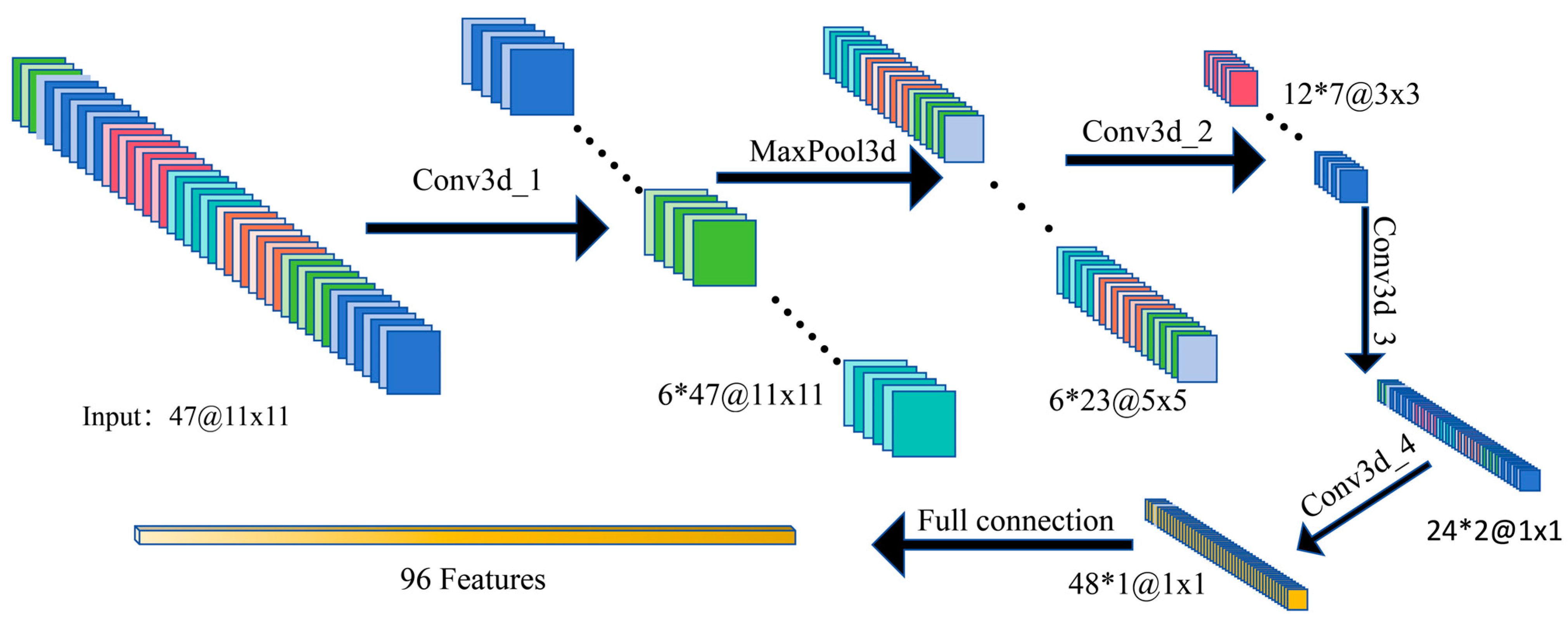
2.3.2. Multi-Level Spatial Feature Extraction

This study also extracted texture, morphological, and deep semantic features from the images to emphasize differences between surface objects for improving classification performance. The gray level co-occurrence matrix (GLCM) algorithm, proposed by Haralick et al. [36], is a powerful and adaptable technique, renowned for its effectiveness in texture extraction. The GLCM algorithm captures the relationship between pixel distances and angles, comprehensively reflecting image information through grayscale correlation calculations between two points in the image. Within the GEE platform, nine common texture features were selected to characterize the GLCM algorithm. These features encompass contrast, entropy, correlation, variance, cluster prominence, inverse different moment, dissimilarity, cluster shade, and angular second moment. Subsequently, principal component analysis (PCA) was employed to reduce the dimensions of multiple texture indices obtained from the GLCM algorithm. PCA was conducted within the GEE platform to compute the principal components for the texture feature objects within the SNIC “clusters” band. The initial three principal components, covering over 90% of the information, were chosen and incorporated into the feature dataset.

Mathematical morphology aims to analyze and process images using mathematical operations. These operations commonly extract, enhance, or modify specific objects or structures in images, such as edges, regions, and contours. Common morphological operations include erosion, dilation, opening, and closing. Erosion and dilation are fundamental operations in morphology. Erosion shrinks the boundaries of objects in an image, eliminating small and insignificant features. Typically, erosion followed by dilation is called opening, and the reverse is closing. Denoting an image as I and a structuring element as SE, the morphological opening and closing of an image with a structuring element are defined as:

$$\mathrm{I}\mathrm{S}\mathrm{E}=\left(\mathrm{I}\mathsf{\Theta }\mathrm{S}\mathrm{E}\right)\oplus \mathrm{S}\mathrm{E},$$

(1)

$$\mathrm{I}·\mathrm{S}\mathrm{E}=(\mathrm{I}\oplus \mathrm{S}\mathrm{E})\mathsf{\Theta }\mathrm{S}\mathrm{E}.$$

(2)

In this study, we conduct PCA dimensionality reduction on the acquired spectral features, resulting in the extraction of the top three principal components. Subsequently, by applying opening and closing operations to four differently shaped structuring elements (line, square, diamond, and disk), we obtain a total of 24 features. After rigorous experimentation, the optimal radius for the structuring elements is found to be 4.

After acquiring various image features, we feed the optimized variables into a convolutional neural network (CNN) for deep feature extraction. Specifically, we use a 3DCNN model built on the PyTorch framework for this task. In Figure 4, Conv3d_1 represents the initial 3D convolutional layer designed to extract primary features from the input data. Padding ensures that the spatial dimensions of the output feature map closely match those of the input to capture boundary information effectively. The MaxPooling layer reduces the spatial dimensions of the feature maps, enhancing features and decreasing computational complexity. Following Conv3d_2, Conv3d_3, and Conv3d_4, continue to extract 96 features. Ultimately, Fc1 transforms the flattened feature map into a 96-dimensional feature set. The network architecture of the 3D CNN is depicted in Figure 4, where a 96-dimensional feature vector is obtained at the fully connected layer and utilized as input for the final classifier.

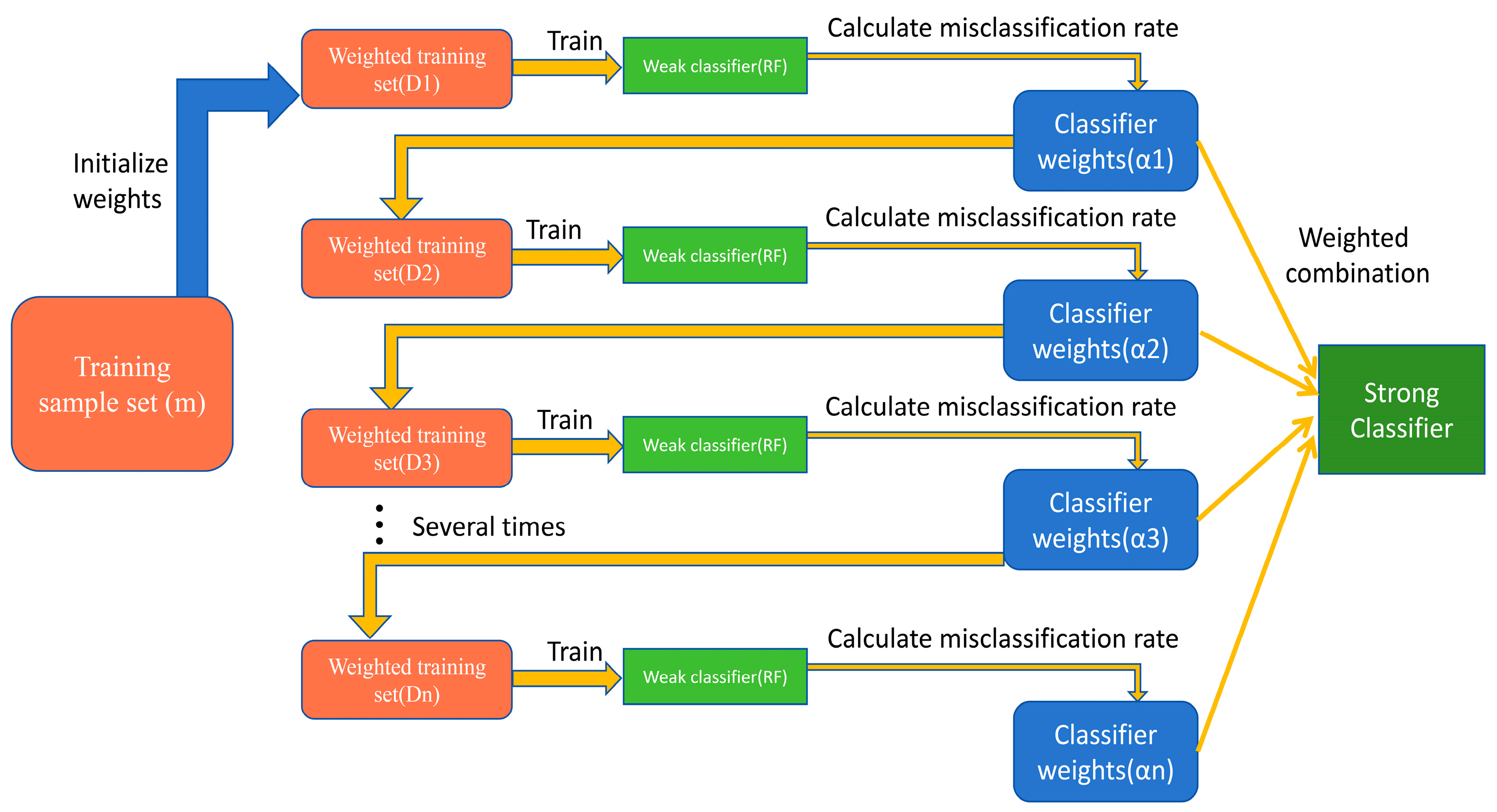
2.3.3. Ensemble Classification

In this study, an ensemble learning classification model based on AdaBoost was designed for land cover classification, where the random forest algorithm was used as the base classifier. Ensemble learning, a machine learning technique, aims to enhance overall performance and prediction accuracy by combining multiple models. Ensemble learning, distinct from reliance solely on a single model, capitalizes on the strengths of multiple models to attain superior generalization and robustness, thereby enhancing its capacity to handle the multifaceted scenarios of big data pertinent to this study. By harnessing the diversity of models to offset the weaknesses or predictive errors of individual models, classification efficiency can be further enhanced.

AdaBoost (adaptive boosting) is a commonly used ensemble model, notable for its adaptability. This feature effectively addresses the multi-feature classification task in this study. The model introduces the random forest classifier as a sub-model in each iteration. Following each iteration, the model dynamically adjusts the weights of misclassified samples from the previous basic classifier, while decreasing the weights of correctly classified samples. These adjusted weights are subsequently utilized to train the succeeding base classifiers. Ultimately, upon reaching the predefined maximum number of iterations, a strong classifier is formed through combination.

The choice of the random forest as the base classifier is due to its long-standing recognition as one of the most commonly utilized algorithms for land cover classification with remote sensing data [37,38,39,40,41,42]. Comparative experiments on previously extracted features consistently demonstrate superior results achieved with the random forest method. Hence, random forest is selected as the base classifier for the final ensemble learning experiment. The ensemble classification method is depicted in Figure 5. Among them, the weak classifier is a sub-classifier. In this experiment, a random forest was ultimately chosen and integrated via ensemble learning to constitute the final strong classifier.

2.4. Experimental Settings

This study conducted feature optimization experiments with the following control groups: (1) Spectral indices + vegetation indices; (2) spectral indices + vegetation indices + terrain factors; (3) spectral indices + vegetation indices + terrain factors + texture features; and (4) spectral indices + vegetation indices + terrain factors + texture features + morphological features. Details are provided in

Table 4. Feature optimization experiments.

Feature Situation		South	East
Serial Number	Number of Features	Total Accuracy	Total Accuracy
Spectral Indices + Vegetation Indices = S1	17	0.9121	0.9207
S1 + Terrain Factors = S2	20	0.9121	0.9236
S2 + Texture Features = S3	23	0.9138	0.9266
S3 + Morphological Features = S4	47	0.9171	0.9320

. Classification experiments were performed using random forest with a decision tree quantity of 80.

For training and validating the 3DCNN model, images were sliced into 256 × 256 segments and input into the neural network. In the 3DCNN network, Conv3d_1 layer utilized convolutional kernels with settings: kernel_size = (5, 5, 5), stride = (1, 1, 1), padding = (2, 2, 2); MaxPooling layer: kernel_size = (2, 2, 2), stride = (2, 2, 2); Conv3d_2 layer: kernel_size = (3, 3, 3), stride = (1, 1, 3); Conv3d_3 layer: kernel_size = (3, 1, 3), stride = (2, 2, 3); Conv3d_4 layer: kernel_size = (1, 2, 2), stride = (1, 1, 2).

For classification using extracted deep learning features, random forest (RF), naive Bayes (NB), and support vector machine (SVM) were chosen as classifiers for experimentation. Random Forest achieved the best results among these classifiers and was subsequently chosen as the base classifier for AdaBoost. Optimal parameters of 300 iterations and a learning rate of 0.1 were determined through experimental testing conducted in this study.

3. Results

3.1. Initial Feature Selection Results and Analysis

The classification method of random forest was employed in this study to obtain the accuracy curve and feature importance ranking as the number of features varied. The accuracy curve, depicted in Figure 6, illustrates a noticeable upward trend until the number of feature variables reaches 16. Beyond this point, the curve exhibits oscillations, leading to the selection of 17 features as the initial set. The 17 initial features include NDWI_mean, NDWI_max, NDBI_mean, NDTI_max, BSI_stdDev, SAVI_max, NDVI_stdDev, NDVI_max and Band 2, Band 3, Band 4, Band 5, Band 6, Band 7, Band 8, Band 11, and Band 12 in Table 1. Among these, “mean” denotes the average value, “max” represents the maximum value, and “stdDev” indicates the standard deviation. Terrain factors consist of slope, aspect, and elevation.

Table 4 displays the optimized feature extraction results. It is evident that incorporating terrain and texture features resulted in a slight accuracy improvement, ranging from 0.1% to 0.3%. Moreover, the addition of morphological features yielded a more pronounced enhancement. Morphological features demonstrate their effectiveness in improving classification accuracy in this experiment.

3.2. Classification Results and Analysis

Quantitative evaluations of classification accuracy using different methods are depicted in Figure 7. AdaBoost-RF integrates deep learning-based feature extraction with Random Forest (RF) as the foundational classifier, subsequently employing AdaBoost for classification. Meanwhile, 3DCNN-NB, 3DCNN-SVM, and 3DCNN-RF employ deep learning for feature extraction, utilizing naive Bayes, support vector machine, and random forest as classifiers, respectively. Results demonstrate that the AdaBoost-RF method, utilizing feature selection via the 3DCNN deep learning model followed by AdaBoost classification, attained overall accuracies of 0.9284 and 0.9383 in the respective experimental regions. Notably, this approach outperformed the other three classifiers, surpassing the 3DCNN-SVM method by 3% and the 3DCNN-NB method by more than 10%. This enhancement can be attributed to the efficacy of Random Forest in managing large input variables and evaluating their significance in category determination. Furthermore, in comparison to the 3DCNN-RF method without ensemble learning, AdaBoost-RF exhibited increases of 0.2% and 0.5% in accuracy in the two experimental regions, respectively, emphasizing the efficacy of ensemble learning classifiers in augmenting the classification performance of base classifiers.

Figure 8 depicts the final classification maps of the South and East experimental areas. Figure 9 depicts the comparative outcomes of different methods in two specific regions, illustrating the land cover and forest distribution achieved through our approach (AdaBoost-RF). The specific positions of case 1 and case 2 in Figure 9 are indicated in Figure 8. Visually, there are no significant misclassifications observed at a large regional scale. Our approach’s results closely match the land cover distribution observed in Sentinel-2 imagery, demonstrating significantly fewer misclassification patches compared to the other three methods. AdaBoost-RF shows a slight improvement in classification accuracy compared to 3DCNN-RF, as shown in Figure 9, accompanied by a decrease in localized misclassifications. Overall, our approach accurately identifies forests in land cover classification results, offering precise spatial distribution of forest resources. This study demonstrates the efficacy of 3DCNN in extracting deep image features, improving classification performance. Ultimately, the integration of deep learning-based feature extractor and ensemble learning classifiers produces the most optimal visual classification outcomes.

This study utilized the proposed approach for nationwide classification. Following repeated experiments in two specific regions, we acquired optimal feature selection results, network models, and parameters. Subsequently, we applied the same methodology to gather nationwide samples and validation data. By employing this approach, we created a national land cover map. Forest resources are crucial natural assets in Czech; thus, our analysis concentrated on forest resources utilizing land classification. Validation points were chosen from the intersection set that had been processed earlier. Unreasonable sample points were eliminated, resulting in the selection of 2563 validation points. As depicted in Figure 10, the results obtained nationwide yielded a total accuracy of 90.98%, the user accuracy of forest is 91.97%, and the producer accuracy is 96.20%. Additionally, user and producer accuracy for other land types were as follows: cropland, 90.51% and 96.60%; grass, 50.00% and 5.48%; shrub, 100.00% and 3.33%; wetland, 0% and 0%; water, 92.31% and 85.71%; impervious, 90.24% and 62.18%.

4. Discussion and Conclusions

4.1. Discussion

This study is subject to certain limitations. For instance, the overall distribution of land in the country results in inadequate sample sizes for categories such as shrub, wetland, and water, leading to unstable classification accuracy. Moreover, while the classification accuracy achieved in our experiment is relatively high, the diversity of the utilized categories is limited. Future efforts will concentrate on exploring methods to refine the classification of forest categories. This can be accomplished by conducting secondary classification of forests using the findings of this study, with a focus on broadleaf forests, coniferous forests, and mixed forests. Furthermore, the data sources utilized in this study solely comprise Sentinel-2 imagery. Future research may involve integrating multiple data sources for classification, leveraging the strengths of each to complement one another and enhance classification accuracy. The 3DCNN model employed in this study effectively handles the issue of multi-spectral input channels for deep learning extraction in convolutional neural networks. Future endeavors may include experimenting with other models, such as ResNet, that utilize three-channel inputs, adjusting channel operations, and integrating attention mechanisms to further enhance classification effectiveness.

4.2. Conclusions

This study proposes a land cover classification method for accurately mapping the spatial distribution of forest resources in Czech. The proposed method fully utilizes 3D convolutional neural networks (3DCNN) and ensemble learning, taking into account feature selection. Initially, the method extracts multidimensional features from remote sensing images, including spectral, texture, morphological, and topographical features. After feature selection, we employ a 3DCNN model to extract deeper semantic information, thereby improving the discrimination of different land cover categories in the imagery. Finally, an AdaBoost-based ensemble learning model is constructed, utilizing the extracted rich features of surface objects as input to achieve the ultimate land cover classification. Two typical regions in Czech are selected as experimental areas for testing the proposed method. This process produces the land classification map in 2018 and obtains the spatial distribution of the Czech forest resources. This study indicates that the utilization of deep neural network models enhances feature extraction capabilities, while ensemble classification methods improve classification results to some extent. This study can serve as a valuable reference for the application of deep learning methods, especially in land cover classification research that incorporates feature selection.

The main conclusions of this study are as follows:

• Feature optimization is particularly crucial for deep learning classification. Our method demonstrates that texture and morphological features enhance remote sensing image classification. These features excel at identifying texture and shape relationships among pixels, thus enhancing image classification within deep learning frameworks. Neural networks excel at extracting features.
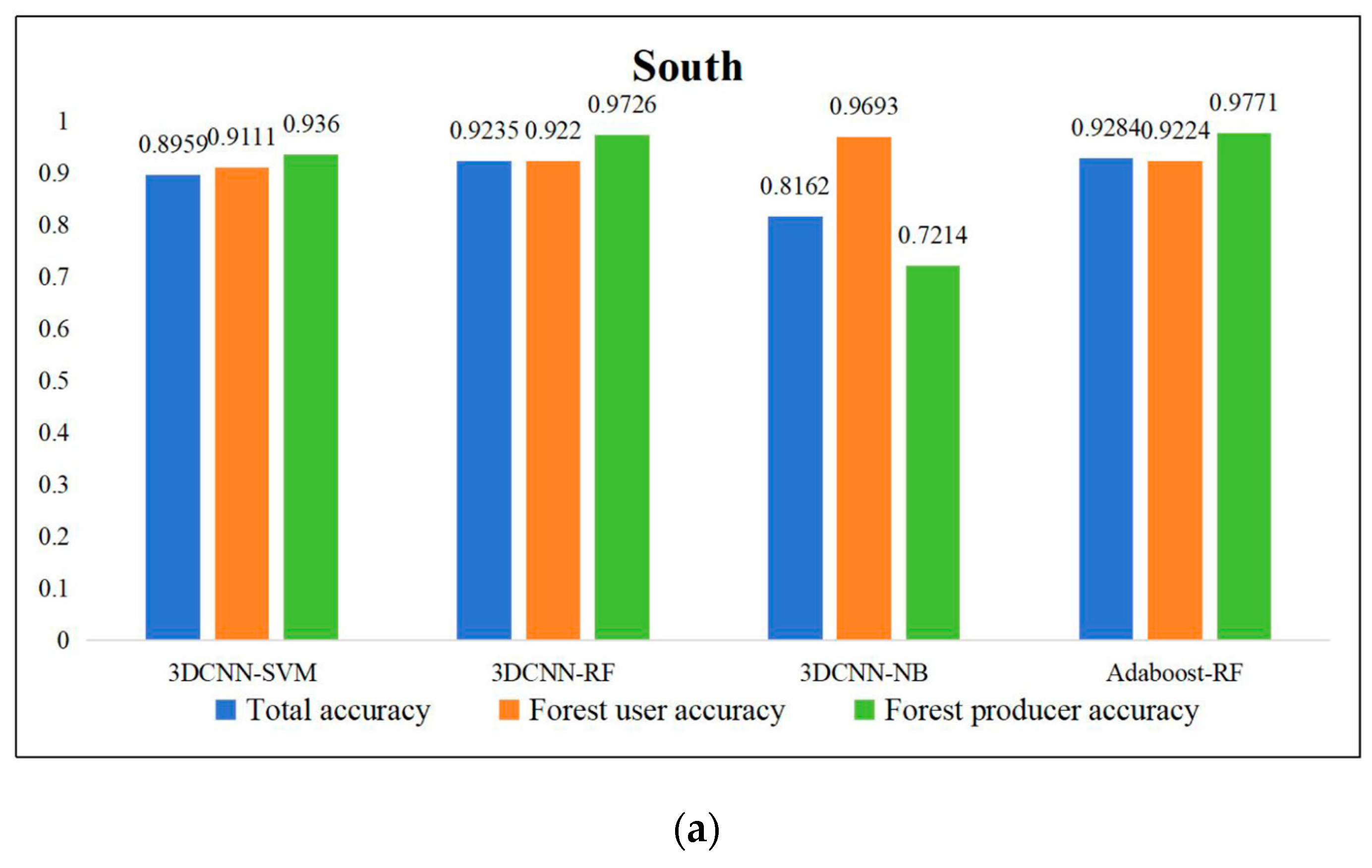
• In multi-band remote sensing image classification methods, random forest outperforms support vector machine and naive Bayes. Random forest inherently handles multi-feature input classification well, resulting in superior classification outcomes in this study compared to support vector machines and significantly outperforming naive Bayesian methods.
• Ensemble learning methods improve the classification of remote sensing images. In two experimental areas, there were varying degrees of improvement. This improvement is attributed to AdaBoost’s automatic adjustment of results in each round, enhancing classification accuracy.

References

1. Lei, J.; Wang, Y.; Huang, J. Review and Prospect of China-CEEC Forestry Cooperation. J. Nanjing For. Univ. 2021, 21, 77–85. [Google Scholar]
2. Wang, Y.; Chen, J.; Gu, Y. Forestry Development in Central and Eastern European Countries and Analysis on Future 16+1 Forestry Cooperation. For. Resour. Wanagement 2017, 153–159. [Google Scholar]
3. Wang, C.; Tian, X. Forest Cover Change Detection based on GF-1 PMS Data. Remote Sens. Technol. Appl. 2021, 36, 208–216. [Google Scholar]
4. Zhang, Z.; Li, Z.; Li, Q.; Hao, R. Dynamic Analysis on Vegetation Coverage Changes of Minqin Oasis Based on GF-1 Remote Sensing Image from 2013 to 2015. J. Southwest For. Univ. 2017, 37, 163–170. [Google Scholar] [CrossRef]
5. Yan, W.; Zhou, W.; Yi, L.; Tian, X. Research Progress of Remote Sensing Classification and Change Monitoring on Forest Types. Remote Sens. Technol. Appl. 2019, 34, 445–454. [Google Scholar]
6. Foody, G.M. The significance of border training patterns in classification by a feedforward neural network using back propagation learning. Int. J. Remote Sens. 1999, 20, 3549–3562. [Google Scholar] [CrossRef]
7. Zhang, S.; Xing, Y.; Aihemaitijiang, A.; Sun, X. Comparison on Forest Type Classification Methods Based on TM Images. For. Eng. 2014, 30, 18–21. [Google Scholar]
8. Mao, L.; Li, M. Integrating Sentinel Active and Passive Remote Sensing Data to Land Cover Classification in a National Park from GEE Platform. Geomat. Inf. Sci. Wuhan Univ. 2023, 48, 756–764. [Google Scholar] [CrossRef]
9. Tan, Q. Spatial Resolution Image: Pixel Versus Object Classification Comparison. J. Basic Sci. Eng. 2011, 19, 441–447. [Google Scholar]
10. Jin, X.; Li, X.; He, B. An improved land cover classification method using multiple features and a support vector machine. Remote Sens. 2018, 10, 1805. [Google Scholar]
11. Honkavaara, E.; Saari, H.; Kaivosoja, J.; Pölönen, I.; Hakala, T.; Litkey, P.; Mäkynen, J.; Pesonen, L. Processing and assessment of spectrometric, stereoscopic imagery collected using a lightweight UAV spectral camera for precision agriculture. Remote Sens. 2010, 2, 5006–5039. [Google Scholar] [CrossRef]
12. Blaschke, T. Object based image analysis for remote sensing. ISPRS J. Photogramm. Remote Sens. 2010, 65, 2–16. [Google Scholar] [CrossRef]
13. Zhu, X.X.; Tuia, D.; Mou, L.; Xia, G.-S.; Zhang, L.; Xu, F.; Fraundorfer, F. Deep Learning in Remote Sensing: A Comprehensive Review and List of Resources. IEEE Geosci. Remote Sens. Mag. 2017, 5, 8–36. [Google Scholar] [CrossRef]
14. Ghamisi, P.; Plaza, J.; Chen, Y.; Li, J.; Plaza, A. Advanced Spectral Classifiers for Hyperspectral Images: A Review. IEEE Geosci. Remote Sens. Mag. 2017, 5, 8–32. [Google Scholar] [CrossRef]
15. He, M.; Li, B.; Chen, H. Multi-scale 3D deep convolutional neural network for hyperspectral image classification. In Proceedings of the 2017 IEEE International Conference on Image Processing (ICIP), Beijing, China, 17–20 September 2017; IEEE: Piscataway, NJ, USA, 2017; pp. 3904–3908. [Google Scholar]
16. Liu, B.; Yu, X.; Zhang, P.; Tan, X.; Wang, R.; Zhi, L. Spectral–spatial classification of hyperspectral image using three-dimensional convolution network. J. Appl. Remote Sens. 2018, 12, 016005. [Google Scholar]
17. Palsson, F.; Sveinsson, J.R.; Ulfarsson, M.O. Multispectral and hyperspectral image fusion using a 3-D-convolutional neural network. IEEE Geosci. Remote Sens. Lett. 2017, 14, 639–643. [Google Scholar] [CrossRef]
18. Mei, S.; Ji, J.; Geng, Y.; Zhang, Z.; Li, X.; Du, Q. Unsupervised spatial–spectral feature learning by 3D convolutional autoencoder for hyperspectral classification. IEEE Trans. Geosci. Remote Sens. 2019, 57, 6808–6820. [Google Scholar] [CrossRef]
19. Sellami, A.; Farah, M.; Farah, I.R.; Solaiman, B. Hyperspectral imagery classification based on semi-supervised 3-D deep neural network and adaptive band selection. Expert Syst. Appl. 2019, 129, 246–259. [Google Scholar] [CrossRef]
20. Roy, S.K.; Krishna, G.; Dubey, S.R.; Chaudhuri, B.B. HybridSN: Exploring 3-D–2-D CNN feature hierarchy for hyperspectral image classification. IEEE Geosci. Remote Sens. Lett. 2019, 17, 277–281. [Google Scholar] [CrossRef]
21. Paoletti, M.E.; Haut, J.M.; Plaza, J.; Plaza, A. Deep learning classifiers for hyperspectral imaging: A review. ISPRS J. Photogramm. Remote Sens. 2019, 158, 279–317. [Google Scholar] [CrossRef]
22. Xia, J.; Ghamisi, P.; Yokoya, N.; Iwasaki, A. Random forest ensembles and extended multi-extinction profiles for hyperspectral image classification. IEEE Trans. Geosci. Remote Sens. 2018, 56, 202–216. [Google Scholar] [CrossRef]
23. Chen, Y.; Wang, Y.; Gu, Y.; He, X.; Ghamisi, P.; Jia, X. Deep Learning Ensemble for Hyperspectral Image Classification. IEEE J. Sel. Top. Appl. Earth Obs. Remote Sens. 2019, 12, 1882–1897. [Google Scholar] [CrossRef]
24. Chi, Y.; Porikli, F. Classification and boosting with multiple collaborative representations. IEEE Trans. Pattern Anal. Mach. Intell. 2014, 36, 1519–1531. [Google Scholar] [CrossRef]
25. Chen, J.; Chen, J.; Liao, A.; Cao, X.; Chen, L.; Chen, X.; He, C.; Han, G.; Peng, S.; Lu, M.; et al. Global land cover mapping at 30m resolution: A POK-based operational approach. ISPRS J. Photogramm. Remote Sens. 2015, 103, 7–27. [Google Scholar] [CrossRef]
26. Zhang, X.; Liu, L.; Zhao, T.; Chen, X.; Lin, S.; Wang, J.; Mi, J.; Liu, W. GLC_FCS30: Global land-cover product with fine classification system at 30m using time-series Landsat imagery. Earth Syst. Sci. Data 2021, 13, 2753–2776. [Google Scholar] [CrossRef]
27. Pflugmacher, D.; Rabe, A.; Peters, M.; Hostert, P. Mapping pan-European land cover using Landsat spectral-temporal metrics and the European LUCAS survey. Remote Sens. Environ. 2019, 221, 583–595. [Google Scholar] [CrossRef]
28. Venter, Z.S.; Sydenham, M.A. Continental-scale land cover mapping at 10 m resolution over Europe (ELC10). Remote Sens. 2021, 13, 2301. [Google Scholar] [CrossRef]
29. Pang, Y.; Meng, S.; Shi, K.; Yu, T.; Wang, X.; Niu, X.; Zhao, D.; Liu, L.; Feng, M.; Qin, X. Forest coverage monitoring in the Natural Forest Protection Project area of China. Acta Ecol. Sin. 2021, 41, 5080–5092. [Google Scholar]
30. Tucker, C.J. Red and photographic infrared linear combinations for monitoring vegetation. Remote Sens. Environ. 1979, 8, 127–150. [Google Scholar] [CrossRef]
31. Huete, A.R. A soil-adjusted vegetation index (SAVI). Remote Sens. Environ. 1988, 25, 295–309. [Google Scholar] [CrossRef]
32. McFeeters, S.K. The use of the Normalized Difference Water Index (NDWI) in the delineation of open water features. Int. J. Remote Sens. 1996, 17, 1425–1432. [Google Scholar] [CrossRef]
33. Van Deventer, A.P.; Ward, A.D.; Gowda, P.H.; Lyon, J.G. Using thematic mapper data to identify contrasting soil plains and tillage practices. Photogramm. Eng. Remote Sens. 1997, 63, 87–93. [Google Scholar] [CrossRef]
34. Rikimaru, A. Landsat TM data processing guide for forest canopy density mapping and monitoring model. In Proceedings of the ITTO Workshop on Utilization of Remote Sensing in Site Assessment and Planning for Rehabilitation of Logged-Over Forest, Bangkok, Thailand, 30 July–1 August 1996; Volume 8, pp. 1–8. [Google Scholar]
35. Chen, Z.; Chen, J. Image recognition analysis and mapping of urban land based on NDBI index method. J. Geo-Inf. Sci. 2006, 8, 137–140. [Google Scholar]
36. Haralick, R.M.; Shanmugam, K.; Dinstein, I.H. Textural features for image classification. IEEE Trans. Syst. Man Cybern. 1973, 6, 610–621. [Google Scholar] [CrossRef]
37. Li, X.; Chen, W.; Cheng, X.; Wang, L. A Comparison of Machine Learning Algorithms for Mapping of Complex Surface-Mined and Agricultural Landscapes Using ZiYuan-3 Stereo Satellite Imagery. Remote Sens. 2016, 8, 514. [Google Scholar] [CrossRef]
38. Millard, K.; Richardson, M. On the Importance of Training Data Sample Selection in Random Forest Image Classification: A Case Study in Peatland Ecosystem Mapping. Remote Sens. 2015, 7, 8489–8515. [Google Scholar] [CrossRef]
39. Cánovas-García, F.; Alonso-Sarría, F.; Gomariz-Castillo, F.; Oñate-Valdivieso, F. Modification of the random forest algorithm to avoid statistical dependence problems when classifying remote sensing imagery. Comput. Geosci. 2017, 103, 1–11. [Google Scholar] [CrossRef]
40. Maxwell, A.E.; Strager, M.P.; Warner, T.A.; Ramezan, C.A.; Morgan, A.N.; Pauley, C.E. Large-Area, High Spatial Resolution Land Cover Mapping Using Random Forests, GEOBIA and NAIP Orthophotography: Findings and Recommendations. Remote Sens. 2019, 11, 1409. [Google Scholar] [CrossRef]
41. Kelley, L.C.; Pitcher, L.; Bacon, C. Using Google Earth Engine to Map Complex Shade-Grown Coffee Landscapes in Northern Nicaragua. Remote Sens. 2018, 10, 952. [Google Scholar] [CrossRef]
42. Teluguntla, P.; Thenkabail, P.S.; Oliphant, A.; Xiong, J.; Gumma, M.K.; Congalton, R.G.; Yadav, K.; Huete, A. A 30-m landsat-derived cropland extent product of Australia and China using random forest machine learning algorithm on Google Earth Engine cloud computing platform. ISPRS J. Photogramm. Remote Sens. 2018, 144, 325–340. [Google Scholar] [CrossRef]
Figure 1. Research area overview.
Applsci 14 02561 g001
Figure 2. Sample distribution. (a) Sample distribution in the East experimental area; (b) sample distribution in the South experimental area.
Applsci 14 02561 g002
Figure 3. Technical flowchart.
Applsci 14 02561 g003
Figure 4. Network structure diagram of 3DCNN.
Applsci 14 02561 g004
Figure 5. Structure of ensemble classification model.
Applsci 14 02561 g005
Figure 6. Accuracy change trend as the number of features changes.
Applsci 14 02561 g006
Figure 7. Comparative experiment on forest classification. (a) Results of South; (b) results of East.
Applsci 14 02561 g007aApplsci 14 02561 g007b
Figure 8. Overall classification maps in the experimental areas.
Applsci 14 02561 g008
Figure 9. Classification maps in the case areas. (a) Case area 1; (b) Case area 2.
Applsci 14 02561 g009
Figure 10. Czech land cover classification map in 2018.
Applsci 14 02561 g010