Article

Applying Geostatistics to Understand Seismic Activity Patterns in the Northern Red Sea Boundary Zone

1
Egyptian National Seismic Network (ENSN), Seismology Department, National Research Institute of Astronomy and Geophysics (NRIAG), Cairo P.O. Box 11421, Egypt
2
Department of Archeology, College of Tourism and Archeology, King Saud University, Riyadh P.O. Box 145111, Saudi Arabia
3
Astronomical, Physical and Mathematical Geodesy (APMG) Group, Institute of Geodesy and Geoinformation, University of Bonn, 53117 Bonn, Germany
*
Author to whom correspondence should be addressed.
Appl. Sci. 2024, 14(4), 1455; https://doi.org/10.3390/app14041455
Submission received: 28 November 2023 / Revised: 26 January 2024 / Accepted: 5 February 2024 / Published: 10 February 2024
(This article belongs to the Special Issue New Challenges in Seismic Hazard Assessment)

Abstract

:
A comprehensive geostatistical analysis was conducted on a dataset comprising 24,321 seismic events in the Red Sea region, spanning from 1997 to 2020. This analysis involved the creation of a new seismic activity database, incorporating data from both Egyptian and Saudi Seismic Networks. This enriched database provided a robust foundation for a detailed examination of the seismic patterns and activities in the region. Utilizing geographic information systems and various spatial analytic methods, it identifies seismic patterns and tectonic influences. The findings reveal significant seismic clustering along the Central Red Sea axis, indicative of active rifting between the Nubian and Arabian plates. The study demonstrates spatial autocorrelation in seismic activities, with high-high clusters marking zones of elevated seismicity. Kernel Density Estimator analyses highlight concentrated seismic activity in the Gulfs of Aqaba and Suez. Higher magnitude events are shown to localize in areas of greater tectonic stress, aligning with known geological features. This research provides critical insights into the seismic dynamics of the Red Sea, showcasing the effectiveness of geostatistical techniques in analyzing seismic data in tectonically active regions.

1. Introduction

The Red Sea is a key crossroads across multiple continents, representing a nexus of geopolitical, economic, and environmental concerns. As a vital maritime artery, this distinctive body of water enhances global trade by offering the most efficient route, thereby playing an essential role in international commerce [1,2]. The ecological significance of the Red Sea is profound. Hosting some of the world’s most diverse coral reefs, it is a vital center for marine biodiversity. Yet, this natural region is under threat from various factors including seismic activity, pollution, and the detrimental effects of climate change [3], underscoring the need for concerted conservation efforts.
Situated within the Afro-Arabian Rift System, the Red Sea region is characterized by significant tectonic activity, resulting from the intricate interactions between the African and Arabian plates [4,5]. These plate dynamics result in various tectonic activities, such as rifting and spreading, increasing the future hazard of the region. The area is structured by significant fault systems including the Red Sea Rift, the Gulf of Suez, and the Gulf of Aqaba [6]. Historical records reported the occurrence of seismic activity in the Red Sea region in 859, 1121, 1191, 1269, 1408, 1630, and 1710 AD, with impacts reaching as far as the Al-Madinah and Makkah Provinces in Saudi Arabia [7,8]. Seismic activity in the Red Sea region, with its proximity to populated areas, presents hazards for neighboring countries, heightening the risk to life and property [9,10].
Observed seismic occurrences are not evenly distributed in the Red Sea tectonic environment, where the rift system is both extended and surrounded by divergent plates. Therefore, in this tectonically active region, it is crucial to understand the spatial and temporal patterns and characteristics of earthquake activities.
The Red Sea region is characterized by seismic activity predominantly featuring small-to-moderate-magnitude earthquakes [7,8]. The study of small-to-moderate-magnitude earthquakes in this region is particularly vital. These events, though less catastrophic than their higher-magnitude counterparts, contribute significantly to the overall seismic hazard due to their higher frequency of occurrence.
Conventional seismic analyses often employ methodologies such as cluster and fractal analyses for spatial data interpretation, and Bayesian information criteria alongside generalized Poisson regression for temporal data analysis. These techniques, while effective in many settings, may not fully capture the complexity of the seismic activity in the Red Sea. Therefore, our study introduces an innovative approach, integrating both spatial and temporal dimensions of seismic data, to provide a more comprehensive understanding of seismic patterns. This methodology is inspired by successful applications in other seismically active regions.
A significant approach for gaining more detailed knowledge of the geodynamic processes in the Red Sea region is through comprehensive analysis of earthquake data over time and space to discern patterns and mitigate future seismic hazards [11,12,13]. These methodologies typically integrate Geographic Information Systems (GIS) with advanced statistical models to map and analyze the distribution and frequency of seismic events. GIS provide a platform for visualizing and analyzing spatial seismic activity data, while statistical models can be used to identify patterns and relationships in the seismic activity enabling identification of risk areas and temporal patterns of seismicity [14,15,16,17]. Understanding spatial and temporal seismic patterns sheds light on the stress distribution and accumulation within the crust, offering insights into the mechanics of earthquake generation and the potential for larger, more damaging events [14]. Those approaches could aid in preparation efforts to identify spatial clusters or concentrated areas of seismic activity [11].
The use of spatial and temporal statistical techniques, like the Average Nearest Neighbor (ANN) analysis [18], is crucial for understanding the spatial distribution of seismic events. By evaluating the average distance between neighboring earthquakes, ANN helps in identifying whether the seismicity is clustered, dispersed, or randomly distributed. This information is crucial for understanding the underlying tectonic processes and for assessing the likelihood of future seismic events in the region. Quadrat Count Analysis (QCA) [19] further complements ANN. This method involves dividing the study area into equal-sized quadrats and counting the number of earthquakes within each. By comparing these counts with a theoretical random distribution, patterns in the spatial distribution of seismicity could be discerned. This technique is particularly useful in the Red Sea region for identifying zones of heightened seismic activity, which may correlate with fault lines. Global Moran’s I (GMI) [20] is a measure of spatial autocorrelation that quantifies how seismic events are related to each other over the entire study area. In the Red Sea, a high GMI value indicates a clustered pattern, which suggests that these seismic events are part of a distributed seismicity, influenced by underlying tectonic processes, rather than occurring in an entirely random manner. This global perspective is essential for a comprehensive understanding of the region’s seismicity. Complementing GMI, Local Moran’s I (LMI) [14,20] provides a more detailed perspective with precise localized clusters of seismic activity. This technique is particularly useful for pinpointing areas within the Red Sea region where earthquake activity is significantly higher or lower than average. LMI can reveal localized seismic hotspots or areas of heightened seismic activity. Integrating results from these methods enhances our understanding of the region’s complex tectonic dynamics. This understanding is invaluable for developing more effective earthquake monitoring, hazard assessment, and mitigation strategies, ultimately contributing to the safety and resilience of the affected regions.
This study explores the transformative role of advanced spatial and temporal statistical techniques in analyzing seismic behavior in the Red Sea region. Focused on small-to-moderate-magnitude earthquakes, which are predominant in this area, our research aims to deepen the understanding of seismic patterns and trends. This enhanced knowledge is critical for assessing and mitigating future seismic hazards or risks. This article aims to pinpoint the spatial localization of seismic hotspots with unprecedented granularity. It demonstrates how methods such as Average Nearest Neighbor (ANN), Quadrat Count Analysis, Global Moran’s I (GMI), and Local Moran’s I (LMI) can be effectively employed to analyze and interpret the spatial and temporal patterns of seismic events in this tectonically active rift system.
The adoption of these techniques serves to elucidate the intricate inner mechanisms that underlie seismic phenomena in the Red Sea area. The Average Nearest Neighbor facilitates the examination of clustering patterns, Quadrat Count Analysis provides insights into the distribution of seismic events, while Global and Local Moran’s I offer a robust assessment of spatial autocorrelation, shedding light on the interconnectivity and localized variations within seismic data.
By achieving this, this article seeks to contribute to a broader understanding of the region’s seismic dynamics, emphasizing the correlation between seismic patterns and underlying geological structures. Additionally, the goals include highlighting the importance of these statistical techniques in enhancing earthquake monitoring and hazard assessment, thus aiding in the development of more robust earthquake preparedness and mitigation strategies. Ultimately, this article strives to provide a comprehensive overview that not only advances academic knowledge but also serves as a practical guide for seismologists and geoscientists working in the field of earthquake research and hazard management.
The structure of the current article is as follows: Section 1 introduces the study’s scope and objectives. Section 2 presents the seismotectonic setting of the Red Sea region. Section 3 describes the research methodology used. Section 4 discusses the experimental design, including data collection and statistical techniques for data analysis. Finally, Section 5 and Section 6 present and interpret the findings, concluding with the study’s contributions.

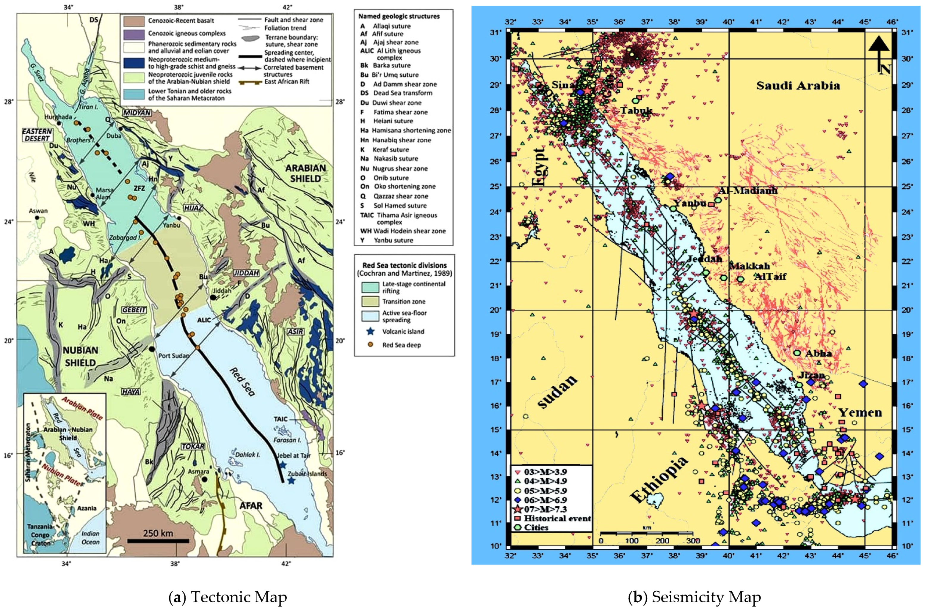
2. Seismotectonic Framework

The Red Sea embodies a significant segment of an expansive rift system that spans multiple geologic features. This region serves as a potential model for understanding the initial rupture of continental lithosphere and its subsequent transformation into oceanic spreading centers, which are key elements in plate tectonics [6].
Recent studies have elucidated the absolute and relative timing of key events in the Red Sea’s geological history, categorizing them into six major phases. The first stage is marked by plume-related basaltic trap volcanism, originating around 31 Ma in Ethiopia, NE Sudan, and SW Yemen, followed by rhyolitic activity near 30 Ma [21]. This early magmatism occurred without any demonstrable extension. The second phase involved marine syntectonic sediment deposition on the continental crust in the central Gulf of Aden between 29.9 and 28.7 Ma, signifying early Oligocene rifting east of Afar [6].
The third phase saw the formation of a small rift basin in the Eritrean Red Sea around 27.5–23.8 Ma, coinciding with extension and rifting within Afar and the creation of the Red Sea as a rift basin. A renewed phase of volcanism characterized the fourth stage, which began around 24–23 Ma. This activity comprised basaltic dikes as well as layered gabbro and granophyre bodies, and extended from Afar and Yemen to northern Egypt. This phase was accompanied by substantial rift-normal extension and deposition of mostly marine and marginal marine syntectonic sediments [4,5].
Regions such as the Gulf of Aqaba and the Dead Sea Rift exhibit elevated and concentrated seismic activity. These areas are tectonically active, linked to the opening of the Northern Red Sea and the Gulf of Aqaba, and also to a major continental strike-slip plate boundary [21,22,23]. The Gulf of Aqaba has experienced left-lateral strike-slip faulting with a 110 km offset from the early Tertiary period to the present. The Arabian Plate boundary extends from the Afar region through the Gulf of Aden, eventually connecting to the Zagros fold belt (see Figure 1a).
The Red Sea region exhibits seismic activity at varying levels in its northern, southern, and central areas, closely linked to its tectonic characteristics. The Gulf of Aqaba and Suez, with their strike-slip faults, are active, and the Red Sea’s axial trough is characterized by concentration of seismic activity, especially at intersections with northeast-trending strike-slip faults [5].
Fault plane solutions from major earthquakes indicate that the region acts as a divergent boundary between the Arabian and Nubian Plates, marked by seafloor spreading northwestward. Seismic activity is predominantly shallow, with over 97% of seismic events in the two Gulfs occurring at depths of less than 10 km. In contrast, seismicity in the Northern and Southern Red Sea varies in depth, suggesting lithospheric deformations in both the upper crust and the uppermost mantle [26,27].
The seismicity in the Red Sea is closely related to the tectonic activities at the spreading center and along the transform faults segmenting the rift. These tectonic forces result in a complex pattern of seismic events, providing a unique opportunity to study the dynamics of plate tectonics, particularly in the context of nascent ocean basin formation.
The seismic activity in the Red Sea is dominated by the complex interplay of tectonic movements due to the rifting and spreading processes. This active tectonic environment generates a spectrum of seismic events, from small tremors to moderate earthquakes. These events are concentrated along the rift where the Arabian and African Plates are moving apart, and along the network of transform faults that segment the rift. Historically, the region has experienced a significant number of seismic events. Between 627 AD and 1955 AD, 88 major and destructive earthquakes were documented [7]. Instrumental records from 1960 to 2020 show 1310 earthquakes with a local magnitude of 4.0 or greater, with only one reaching a magnitude of 7.1, while the rest were below this magnitude (Figure 1b) [17,27,28].

3. Related Work and Methodology

Traditional seismological techniques have been employed to study seismic activity in tectonically complex areas. The emergence of geospatial statistical evaluation, however, has significantly enhanced our analytical capabilities. This multidisciplinary approach offers detail and flexibility in analyzing seismic activity data [14]. To identify statistically significant patterns in seismic activity data, a series of analyses employing four distinct techniques was conducted. These methods have been effectively utilized in numerous studies across the globe, including Romania [29], Indonesia [30], the Red Sea [14], China [31], and Pakistan [32]. It has consistently yielded valuable insights into areas of heightened seismic activity, spatial configurations of earthquake events, and the spatiotemporal dynamics, mechanisms, and characteristics of seismic activity [33]. The approach and statistical method applied in this study are novel in their application to identifying patterns in the spatial distribution of seismic events in the Red Sea. The statistical approaches employed and detailed in subsequent sections play a crucial role in revealing the spatial relationships and intrinsic patterns within the Red Sea region.

3.1. Average Nearest Neighbor (ANN)

The Average Nearest Neighbor (ANN) method is a widely used technique in spatial statistics to analyze the pattern of a set of earthquakes within a given space. It provides a measure to determine whether the earthquake epicenter pattern exhibits clustering, randomness, or uniformity [14,18,34,35]. To define the ANN method, consider a set of  n  earthquake epicenters in the Red Sea region. The method computes the distance from each earthquake to its nearest neighbor, resulting in  n  distances. The average of these distances, denoted as  D ¯ , is compared to the expected average distance for a random pattern,  E D , in the Red Sea region of the same size and shape. The ratio of these two distances is used to quantify the earthquake pattern [36]:
R = D ¯ E D
The expected average distance  E D  in a random distribution can be estimated for a two-dimensional space with uniform point distribution using the formula [18]:
E D = 1 2 λ
where  λ  is the density of earthquakes (number of earthquakes per unit area) in the Red Sea region. The value of  R  indicates the nature of the earthquake pattern: If  R = 1 , the pattern is considered random. If  R < 1 , the earthquakes are more clustered than expected in a random pattern. If  R > 1 , the earthquakes are more regularly spaced (uniformly distributed) than expected in a random pattern. This method is simplistic yet powerful in assessing spatial earthquake patterns.

3.2. Quadrat Count Analysis (QCA)

Quadrat Count Analysis is a statistical tool used in the study of spatial patterns. It is particularly useful in seismology for analyzing the distribution of earthquake epicenters. The methodology involves dividing the study area into smaller, non-overlapping subareas of equal size, known as quadrats [19]. The number of seismic events occurring within each quadrat is then tallied, producing a discrete spatial frequency distribution of counts. The variance-to-mean ratio (VTMR) or the index of dispersion is used to evaluate the pattern of seismic activity in the Red Sea region. The VTMR is a dimensionless number that serves as a test statistic for the spatial randomness of observed seismic events. It is defined as the variance of the quadrat counts divided by the mean count [19,37]:
V T M R = σ 2 μ
where  σ 2  is the variance of the quadrat counts, and  μ  is their mean. In a completely random spatial process adhering to a Poisson distribution, the VTMR would be approximately equal to one. Deviations from this value indicate non-random patterns. Specifically, a VTMR greater than one suggests clustering, while a value less than one indicates a regular or overdispersed distribution. The significance of the observed VTMR is further evaluated using the Z-score, which measures the number of standard deviations the observed VTMR is from the expected value under the null hypothesis of spatial randomness [38]. The Z-score is given by:
Z = V T M R 1 2 n
where  n  is the number of quadrats. A high absolute value of the Z-score indicates that the null hypothesis can be rejected, implying a substantial departure from spatial randomness. The p-value associated with the Z-score quantifies the likelihood of observing a VTMR as extreme as, or more extreme than, the one calculated under the assumption that the null hypothesis holds true. A low p-value (typically less than 0.05) leads to the rejection of the null hypothesis, affirming the presence of a statistically significant spatial pattern [39].

3.3. Global and Local Moran’s I

Spatial autocorrelation is an important index to express the spatial behavior of geographical elements, reflecting the interdependence between some elements in the study area [30]. The global indicators of spatial association, such as Global Moran’s I, and the Local Indicators of Spatial Association (Local Moran’s I, also known as LISA), are frequently employed to quantify spatial autocorrelation [33]. These metrics, Global and Local Moran’s I, are robust analytical techniques that offer valuable insights into the spatial structures and associations inherent in geospatial datasets. Their application extends across various domains, offering a quantitative basis for spatial pattern analysis and decision making [39]. Both Global and Local Moran’s I play a pivotal role in spatial analysis, contributing to a comprehensive understanding of the distribution of earthquake epicenters. They assist in unraveling the spatial dynamics and patterns, which are crucial for informed policy making and resource allocation decisions [40].

3.3.1. Spatial Weight Matrix

The estimation of a spatial weight matrix is essential in the context of Global and Local Moran’s I analysis. This matrix defines the spatial relationships between individual data points, specifying which observations are neighbors and to what extent they influence one another within a given geographic area. Thus, the accurate estimation of the spatial weight matrix is a crucial prerequisite for meaningful spatial analysis and the interpretation of results [41]. In this study, the spatial weight matrix characterizes the interactions between geographical earthquake epicenters, primarily predicated on the proximity or contiguity of the mapped areas. Spatial weights are formulated based on the adjacency connections among these territories [42]. The construction of these weights is defined as follows:
μ = μ 11 μ 12 μ 1 m μ 21 μ 22 μ 2 m μ m 1 μ m 2 μ m m
where m represents the number of regions, and  μ i k  indicates the spatial adjacency relation between regions i and k.

3.3.2. Global Moran’s I (GMI)

Global Moran’s I (GMI) is a statistical measure used to assess spatial autocorrelation in geospatial data. Spatial autocorrelation refers to the degree to which a set of spatial features and their associated data values are correlated with themselves in space. In essence, it evaluates whether the pattern expressed is clustered, dispersed, or random [39]. The Global Moran’s I is mathematically defined as [43]:
I = N i j w i j i j w i j X i X ¯ X j X ¯ i X i X ¯ 2
where  N  is the number of spatial units indexed by  i  and  j X i  and  X j  are the values of the variable of interest for spatial units  i  and  j X ¯  is the mean of  X , and  w i j  is the spatial weight between units  i  and  j .
This statistic falls in the range of  1 , 1 , where a value close to +1 indicates clustering, −1 indicates dispersion, and a value around 0 implies randomness.

3.3.3. Local Moran’s I

Local Moran’s I (LMI), is a statistical measure used to assess the spatial autocorrelation of data within a geographic area. It identifies and quantifies the degree to which individual data points are clustered or dispersed in relation to their neighboring data points. The Local Moran’s I for a location  i  is given by [43]:
I i = X i X ¯ S 2 j w i j X j X ¯
where  S 2  is the variance of  X , and the other terms are as defined previously. The significance of Local Moran’s I values is typically assessed through permutation tests, providing insights into the local structure of the spatial correlation. High positive values suggest clusters of similar high or low values, while negative values indicate spatial outliers.
While the GMI provides an overall measure of spatial autocorrelation, it does not allow for the detection of local patterns of spatial association. Local Moran’s I (LMI), also known as the Local Indicators of Spatial Association (LISA), identifies clusters of similar values and outliers in spatial data [39,44]. LISA are applied to depict the spatial dynamics of earthquake hazard. LISA cluster the mapped region into different clusters. High-high (H-H) areas are characterized by high concentrated seismic activity and are surrounded by regions with similarly high seismic hazard indices. In contrast, low-high (L-H) areas exhibit potentially low seismic hazard, yet are encircled by regions with high seismic hazard. Low-low (L-L) regions have low seismic hazard and are bordered by areas with corresponding low indices. Finally, high-low (H-L) areas display high seismic hazard but are surrounded by regions with lower seismic hazard levels. Utilizing these classifications, LISA evaluate the seismic hazard of earthquakes at a significance level of p = 0.05, and those provinces, autonomous regions, or municipalities that surpass this threshold are subsequently illustrated on a LISA cluster map. The mathematical expression for LISA is structured as follows [44]:
I i = η i η ¯ S 2 k = 1 m μ i k η k η ¯ i k ; i , k = 1 , 2 , , m
where  S 2 = 1 m i = 1 m η i η ¯ i = 1,2 , , m , and  I i  represents the local autocorrelation index.

3.4. Categorization of Concentrated Activity Areas

The categorization of hotspots or areas of heightened seismic activity using Getis-Ord Gi* and Kernel Density Estimation (K) involves a two-step process to identify and classify spatial patterns in a dataset. First, Getis-Ord Gi* is employed to detect statistically significant hotspots or coldspots (areas of elevated or diminished seismic activity in the Red Sea region) within the data. This statistic assesses the spatial clustering of high or low values and provides a measure of significance for each location. Positive Gi* values indicate hotspots of high concentrated seismic activity, while negative values indicate coldspots or dissipated seismic activity areas [45]. Second, Kernel Density Estimation (K) is utilized to create a smoothed density surface that highlights areas of high data concentration. This helps in visualizing the intensity and extent of the intensified seismicity identified by Getis-Ord Gi*. Kernel Density Estimation provides a continuous representation of spatial patterns, allowing for a more nuanced understanding of the data distribution.

3.4.1. Getis-Ord Gi*

The Getis-Ord Gi* statistic is a measure used to assess the degree of spatial clustering of values within a geospatial seismicity dataset. It is valuable for identifying areas with heightened or diminished seismic activity [46] of high or low earthquake magnitude values. The formula for calculating the Getis-Ord Gi* statistic is as follows [45]:
G i * d = j = 1 n w i j x j x ¯ j = 1 n w i j j = 1 n x j 2 j = 1 n x j 2 n 1
where  G i * d  represents the Getis-Ord Gi* statistic at a given distance threshold  d n  is the total number of spatial units or observations.  x j  represents the value of the variable of interest at spatial unit  j x ¯  represents the mean of the variable across all spatial units.  w i j  represents the spatial weight between spatial units  i  and  j , typically based on distance.
The Getis-Ord Gi* statistic evaluates whether the observed spatial clustering of high or low values is significantly different from what would be expected under spatial randomness. Positive values of Gi* denote spatial clustering of high values, indicative of concentrated areas with heightened seismic activity. Conversely, negative values signify clustering of low values, highlighting regions with diminished seismic activity [46].

3.4.2. Kernel Density Estimation (K)

Kernel Density Estimation (K) is a statistical technique used to estimate the probability density function of a continuous random variable from a set of data points [47]. It is particularly valuable for visualizing data distribution in a non-parametric way [48]. The formula for Kernel Density Estimation is as follows [49]:
f ^ x = 1 n i = 1 n K x x i h
where  f ^ x  represents the estimated probability density function at point  x n  is the total number of data points.  x i  represents each data point.  K u  is the kernel function, which is a symmetric probability density function (such as the Gaussian or Epanechnikov kernel).  h  is the bandwidth parameter, which determines the width of the kernel and affects the smoothness of the estimated density. In this equation, the kernel function is centered at each data point  x i  and scaled by the bandwidth  h . The kernel functions are summed up and normalized by  n  to create a smooth estimate of the underlying probability density function.

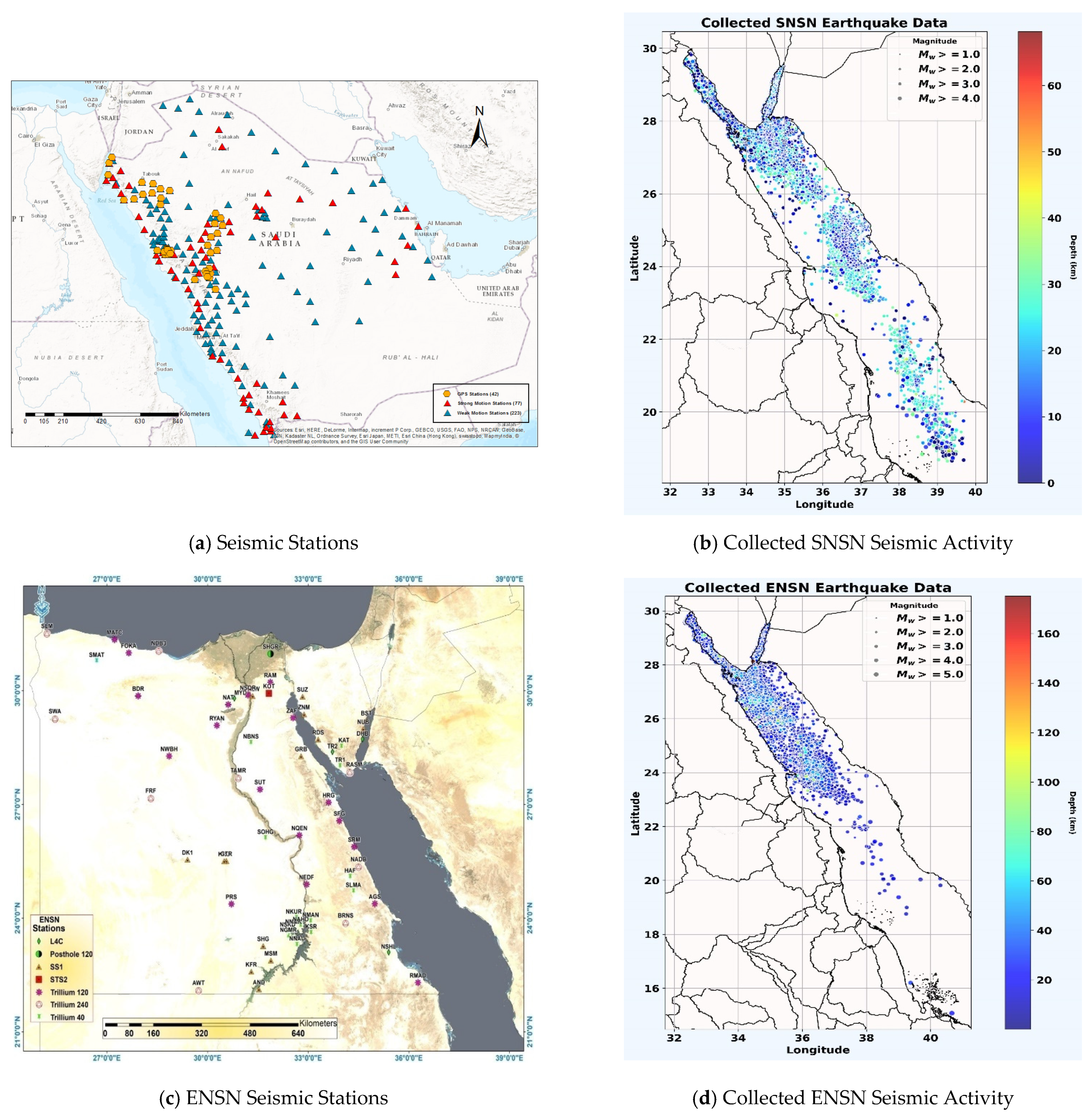
4. Experimental Design

This research utilizes four statistical methods, all integrated into an advanced geospatial computational framework. These methods are employed to examine the temporal and spatial patterns of earthquake occurrences in the Red Sea region. For this study, we compiled comprehensive seismic data from both Saudi and Egyptian seismological networks, encompassing a range of time periods to develop an extensive seismicity catalog database. The Saudi dataset for this research is sourced from the Saudi Geological Survey (SGS), which has managed the Saudi National Seismic Network (SNSN). The SGS began deploying broadband seismic stations in 2004, and subsequently controlled the seismic stations from the King Abdulaziz City for Science and Technology (KACST) and King Saud University (KSU), following a directive from the Saudi Council of Ministers. Seismic data were collated from KSU (up to 2003), KACST (2004–2005), and SGS (2006–2020). The second pivotal dataset was acquired from the Egyptian National Seismological Network (ENSN), managed by the National Research Institute of Astronomy and Geophysics (NRIAG). The ENSN has played a crucial role in capturing a range of seismic events in the Red Sea area, documenting earthquakes with diverse magnitudes and characteristics. The ENSN’s data, covering the period from 1998 to 2022, are integral to this study.
The spatial configurations of seismic stations within both the SNSN and ENSN are detailed in Figure 2a and Figure 2c, respectively. Concurrently, the spatial distribution of the collected seismic events captured by these networks is illustrated in Figure 2b,d.
In our study, the seismic data from the southern section of the Red Sea, specifically below latitude 18–19 N, have been deliberately excluded from the final database. This decision was driven by the notable disparity in data availability between the two data sources of the Red Sea. As clearly illustrated in Figure 2b, the Egyptian side of the Red Sea, encompassing the southern section, offered limited seismic data. In stark contrast, the Saudi side provided a more robust and comprehensive dataset. This uneven distribution of data led to the decision to exclude the southern section from our analysis, ensuring that our study was based on a dataset that was both reliable and adequately representative of the seismic activities we aimed to investigate. This methodological choice was essential to maintain the scientific rigor and accuracy of our findings, despite the geographical limitation it imposed.
Table 1 offers a detailed statistical summary of the datasets from the ENSN and the SNSN. It includes important statistics like the total count, mean, standard deviation, and range for different temporal and spatial parameters of seismic events. These parameters cover the date and time of each event (year, month, day, hour, minute, second) and geographical details (latitude, longitude, depth, magnitude). Collecting these data shall help in understanding the distribution, central tendency, and variation of seismic activities within the mapped area.
Based on the spatial distribution depicted in Figure 2 and the summary statistics presented in Table 1, it is evident that the collected ENSN and SNSN datasets closely align in terms of their sample sizes. Specifically, ENSN comprises 50,747 earthquakes, while SNSN encompasses 51,531 events. While the ENSN data are more current, covering the period from 1998 to 2022, SNSN offers a longer temporal span, ranging from 1988 to 2020. This is further substantiated by the average year of recorded events: ENSN’s mean year is 2008, slightly more recent than SNSN’s 2005 (Table 1), implying temporal variations in data collection. In spatial terms, both datasets encompass similar geographical extents. However, SNSN exhibits a broader distribution, as evidenced by its higher mean latitude of  27.64 °  and longitude of  35.01 ° , compared to ENSN’s mean latitude of  26.72 °  and longitude of  34.80 ° . The ENSN dataset has a slightly lower standard deviation in latitude and longitude, which reflects a more concentrated area for data collection. This is supported by the geographical distribution of the seismic stations employed in both networks. Daily temporal distribution is consistent in both datasets, although ENSN has a marginally higher mean hour of 12.17, compared to SNSN’s 11.67. Depth and magnitude reveal further distinctions; the depth of seismic events in ENSN tends to be deeper on average (15.42 km) with a higher variance (7.52) compared to SNSN (13.57 km, std: 8.24). ENSN’s records penetrate deeper into the Earth’s crust, with a maximum depth of 75.19 km, and also display more intense seismic events, peaking at a magnitude of 5.7. In contrast, SNSN’s data primarily encompass events of moderate depth and magnitude, with averages of  13.57  km and  1.61 , respectively.
Following data collection, each seismic event was carefully categorized based on parameters including annual frequency, magnitude range, and depth variations. These consolidated data were then integrated into a unified GIS database. In the process of consolidating the ENSN and SNSN catalogs, a multifaceted approach was employed to ensure data integrity and compatibility. Initially, both catalogs were subjected to a rigorous investigating to remove non-tectonic seismic events, specifically focusing on the exclusion of quarry blasts utilizing the ZMAP software version 7 [52]. Subsequently, statistical outlier detection methods, such as the Modified Z-score [53], were applied to remove anomalous events with aberrant magnitudes or locations or depths. To tackle the issue of disparate local magnitude ( M l ) scales, a unifying transformation was executed to convert all reported magnitudes to moment magnitude ( M w ). To standardize magnitude measurements across datasets, all values were normalized to the moment magnitude scale ( M w ). This was facilitated by a series of empirically derived conversion equations, each tailored to the specific seismological characteristics of the corresponding network. This standardization relied on the  M w  scale’s proven reliability and employed conversion relations delineated by Moustafa et al. [35] for ENSN data and by Babiker et al. [54] for SNSN data. Finally, the homogenized datasets were merged, thereby producing a comprehensive, unified seismic catalog with uniform magnitude reporting. Figure 3 depicts the spatial distribution of selected seismic events. Meanwhile, Table 2 provides descriptive statistics for each of the dataset’s parameters.
In the following procedural outline, we detail the methodological steps for merging seismicity catalogs obtained from the Saudi Seismic Network and the Egyptian Seismic Network. This algorithm systematically guides the integration of seismic event data from these two distinct sources, emphasizing data accuracy, quality control measures, and conflict resolution to create a consolidated and standardized seismicity catalog:
  • Saudi Seismic Network Catalog:
    • Import the seismic data from the Saudi Seismic Network catalog.
    • Identify unique events using distinctive event identifiers, such as event IDs and timestamps.
    • Exclude redundant events within to streamline the dataset.
  • Egyptian Seismic Network Catalog:
    • Import seismic data from the Egyptian Seismic Network catalog.
    • Identify events unique to Egyptian catalog using specific event identifiers for cross-referencing.
    • Eliminate redundant events within Egyptian catalog to enhance data clarity.
  • Common Event Identification:
    • Determine seismic events that exist in both catalogs, employing event identifiers.
    • Exclude duplicate events shared between the Saudi Seismic Network and the Egyptian Seismic Network catalogs.
  • Merge Process:
    • Combine the remaining unique events from both catalogs to create the merged seismicity catalog.
    • Ensure the accuracy of metadata by updating information such as event location, magnitude, and depth.
  • Quality Control Measures:
    • Implement rigorous quality control checks to address potential discrepancies and maintain data accuracy.
    • Resolve conflicts arising from discrepancies in seismic event information between the two catalogs.
  • Conflicting Data Strategy:
    • Use 10 s origin time difference and 10 km epicentral distance difference between the two catalogs to manage conflicting data, prioritizing information from either the Saudi Seismic Network or the Egyptian Seismic Network.
    • Utilize additional data sources to resolve conflicts and ensure data consistency.
  • Data Format Standardization:
    • Standardize the format of the merged seismicity catalog to ensure uniform representation.
    • Preserve the integrity of data presentation for subsequent analysis.
  • Documentation:
    • Document the merging process, including steps taken to resolve conflicts, quality control measures, and updates to metadata.
    • Provide a clear record of the synthesis of seismic data from the Saudi Seismic Network and the Egyptian Seismic Network catalogs.
  • Validation Checks:
    • Perform validation checks on the merged catalog to confirm the success of the merging process.
    • Ensure that the resulting dataset aligns with expectations and maintains data integrity.
  • Final Review:
    • Conduct a final review of the merged catalog to verify compliance with standards and the inclusion of all relevant seismic events.
    • Confirm that the merged dataset effectively represents the seismic activity captured by both the Saudi Seismic Network and the Egyptian Seismic Network.
  • Save and Export:
    • Preserve the final merged seismicity catalog in the desired format for subsequent analytical endeavors.
Figure 3 displays the geographic distribution of seismic activity in the Red Sea, emphasizing the spatial concentration of earthquakes. This concentration is aligned along certain longitudinal and latitudinal lines, indicative of fault zones. These zones reveal where tectonic stress accumulates and is episodically released, typically near tectonic boundaries. Areas with reduced seismic activities are highlighted, suggesting more stable tectonic regions. Such distribution patterns offer insights into the region’s tectonic dynamics. Furthermore, two cross-sectional views detailing the depth profiles of these earthquakes relative to latitude and longitude are depicted. This perspective provides a comprehensive understanding of the seismic activity’s vertical extent. Variations in earthquake depth may reflect differences in the crust or lithospheric layer’s composition or rheology within the Red Sea. The clustering of earthquakes at specific depths could indicate distinct faulting mechanisms, each associated with its characteristic depth range. The occurrence of deeper earthquakes might signify an interaction zone between the mantle and crust. These depth-related observations are integral to grasping the complex geodynamics of the Red Sea area.
Table 2 presents data on 37,730 seismic events recorded in the Red Sea region from 1997 to 2020. The table combines the temporal and spatial attributes of earthquakes from the ENSN and SNSN datasets. The data span 23 years, indicating a temporal distribution with an average occurrence year of 2006. This central point suggests a concentration of seismic activities around this period, although the standard deviation of 3.93 years shows a wide spread over two decades. The dataset’s temporal consistency is evident in its even distribution across months, days, hours, and minutes, with standard deviations within normal ranges, indicating no significant time-based anomalies. Geographically, the mean coordinates are  27.15 ° N and  34.88 ° E, aligning closely with the individual dataset averages. The small standard deviations in latitude and longitude confirm a consistent geographical focus. The average earthquake depth of 15.04 km, with a standard deviation of 6.85 km, underlines the tectonic dynamics of the Red Sea and the variability in seismic event depths. The moment magnitude ( M w ) has an average of 1.66 and a standard deviation of 0.51, ranging from 1.00 to 3.20. This range suggests a predominance of low-to-moderate-magnitude earthquakes, with only a fraction exceeding a magnitude of 2. The absence of extremely high-magnitude events is noteworthy. Additionally, the quartile distribution aligns the median depth and magnitude with their means, indicating a near-symmetrical distribution. This symmetry could simplify statistical modeling by reducing the need for non-linear transformations to achieve data normality.

5. Statistical Characterization of Seismic Activity

Investigating the statistical characteristics of earthquakes in the Red Sea region is essential for comprehending seismic activity and crustal deformation in rift zones. The examination of the temporal progression and geographical dispersion of seismic events is vital for deciphering patterns of stress accumulation and release. Such insights are useful in advancing seismic forecasting and hazard management strategies [17]. Moreover, the analysis of small-to-moderate-magnitude earthquakes provides valuable information on the initial stages of seismic processes, which is crucial for enhancing preparedness and mitigation efforts [55].

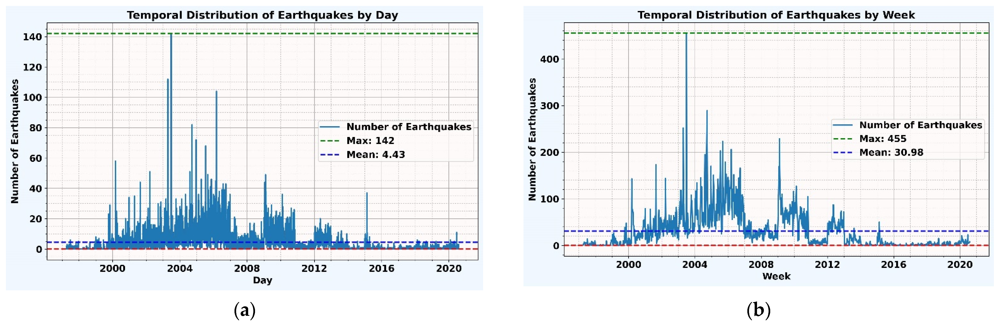
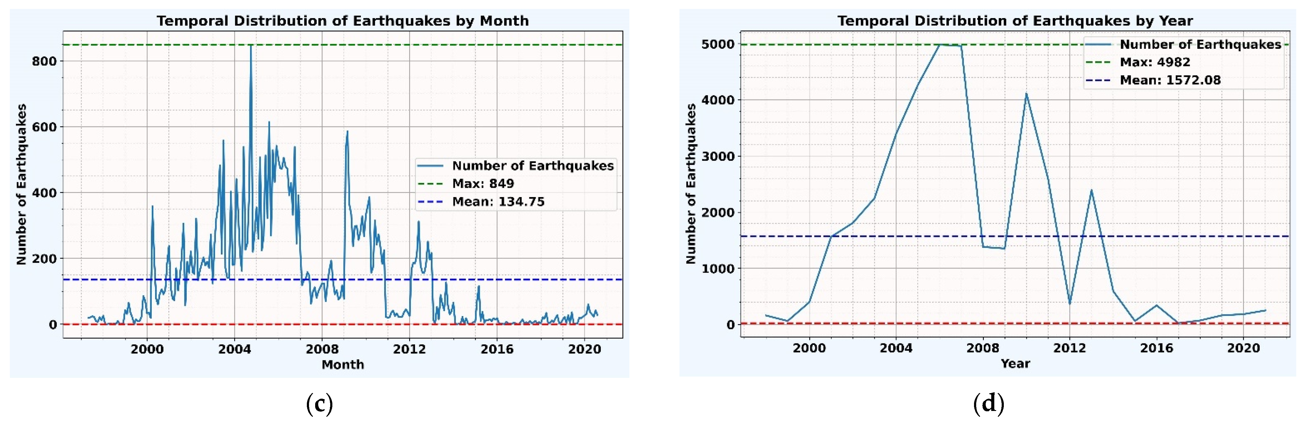
5.1. Temporal Patterns

To gain insight into the development of seismic activity in the Red Sea region, the temporal distribution of earthquakes was analyzed across multiple scales, as depicted in Figure 4. Each plot in this figure is tailored to assess earthquake frequency at specific time resolutions, including daily, weekly, monthly, and yearly intervals. Figure 4a sheds light on daily changes, revealing a non-uniform distribution of seismic activity. The daily peak frequency reaches 142 seismic events, while the mean frequency is about 4 events per day. This variability in daily event counts may be indicative of episodic clusters of seismic activity, possibly influenced by underlying tectonic processes. The data reveal that it is somewhat quieter at night in most places. Turning to a weekly seismic activity, Figure 4b illustrates the weekly irregularity of the reported earthquakes. The plot shows a weekly peak of 445 earthquakes, compared with an average frequency of 30 events per week. The range of weekly event counts is quite broad. This significant variability indicates that the region undergoes periodic episodes of increased seismic activity, likely influenced by underlying tectonic interaction processes. Figure 4c presents the observed monthly distributions, highlighting any potential seasonal cycle patterns. These could possibly be linked with geological processes like rifting affecting the area. The reported activity records a high monthly frequency of 849 earthquake events, with an average rate of 134 events per month. This variability in monthly seismic activity suggests the presence of complex temporal dynamics, possibly punctuated by bursts of heightened seismic events. The substantial spread in the number of events, as captured by the standard deviation, indicates that the seismic behavior in the Red Sea region is not uniformly distributed over time, perhaps influenced by episodic tectonic activities or other underlying geophysical processes. Lastly, on an annual scale, Figure 4d includes the yearly distribution, exhibiting multi-year patterns. The annual data indicate a peak of 4982 earthquakes, with a mean incidence of 1572 occurrences each year. The data suggest that seismic activity in the area is not constant over various years, underlining the necessity for long-term monitoring and study to understand the underlying dynamics.
The analysis of temporal patterns suggests that the Red Sea region displays a consistent level of seismic activity. The distribution over time does not reveal a clear trend of increasing or decreasing seismic events across the observed years; instead, the activity fluctuates. There are noticeable periods of more frequent seismic events, as indicated by clusters of taller bars in the data. Pronounced spikes representing days with exceptionally high activity could correspond to significant seismic occurrences or sequences, such as swarms of earthquakes or series of aftershocks. These findings corroborate the results of several previous studies [5,8,56,57].

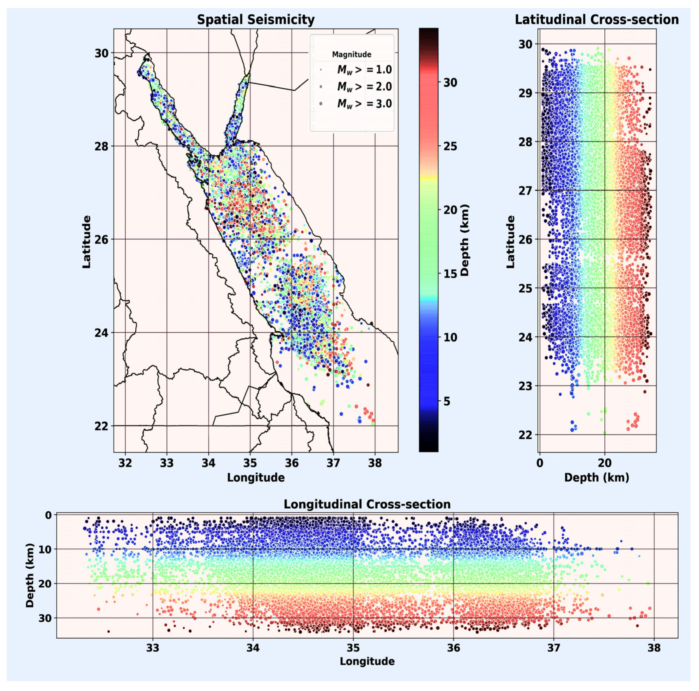
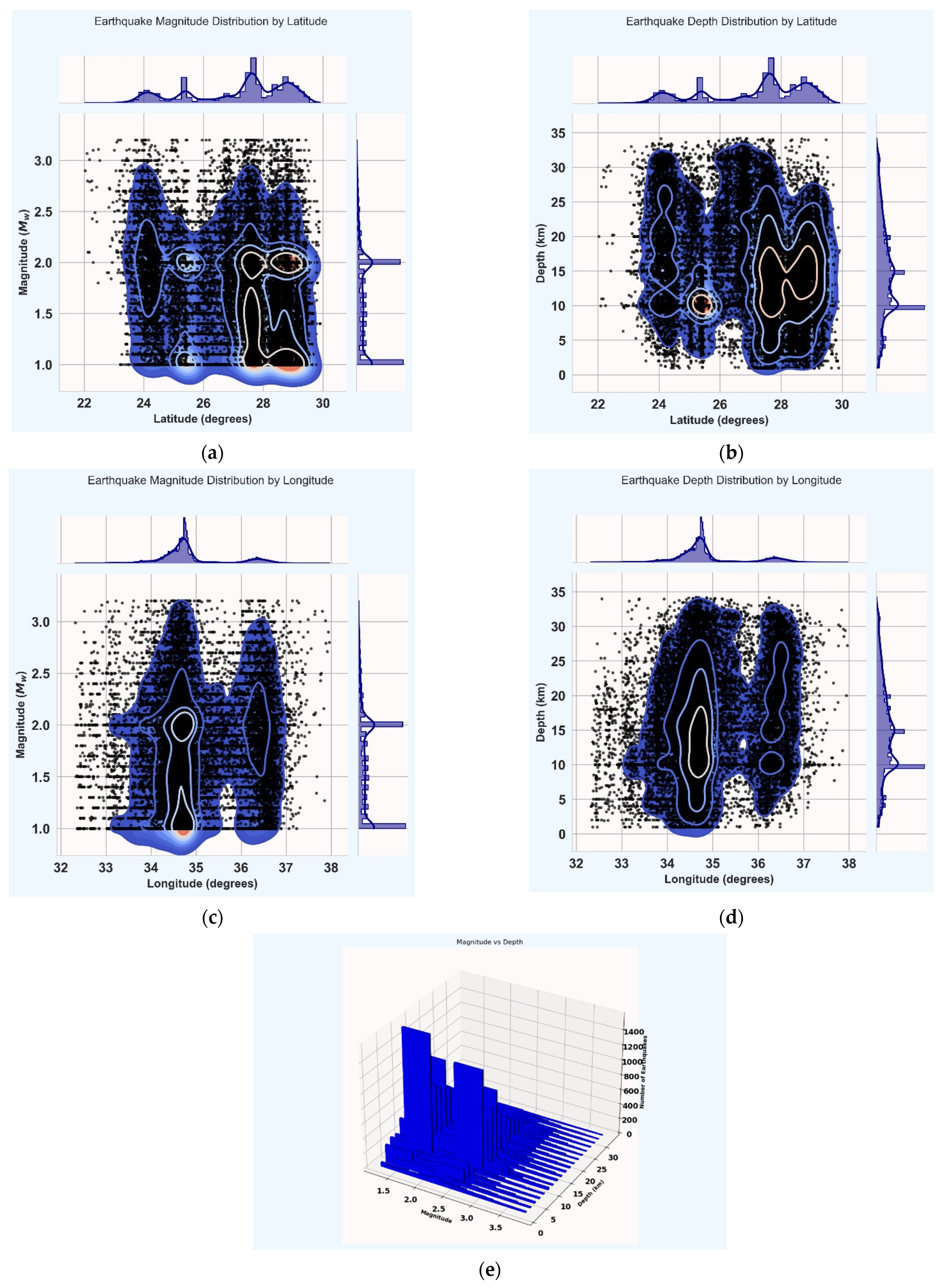
5.2. Spatial Distribution

Understanding seismicity patterns is fundamentally linked to the spatial distribution of earthquake moment magnitudes ( M w ) and the variability of depth in relation to latitude and longitude, as depicted in Figure 5. Moment magnitude combined with depth offers crucial insight into the geodynamic processes that shape the Earth’s crust.
Figure 5 displays a density plot that illustrates the distribution of earthquake moment magnitudes ( M w ) and depths in relation to either latitude or longitude. Figure 5a illustrates a concentration of seismic events with magnitudes predominantly clustered between latitudes of 24 and 28 degrees, indicating a zone of heightened seismic activity within this range. The accompanying marginal histogram exhibits pronounced peaks that correspond to the densest areas, revealing that most earthquakes occur with magnitudes between 1.5 and 3.0  M w .
These observations suggest that seismic activity is not uniformly distributed but is instead focused in specific regions, potentially aligning with underlying geological structures such as tectonic plate boundaries or rift zones. Figure 5b indicates that the deepest earthquakes are concentrated around latitudes of 25 to 26 degrees and 28 to 29 degrees, hinting at a potential correlation with geologically active events. The marginal histograms demonstrate that the majority of seismic events take place at depths of less than 10 km, with a decline in frequency at greater depths. Figure 5c highlights a notable concentration of seismic activity, particularly of lower magnitudes, around a 35-degree longitude.
The marginal histograms exhibit a pronounced spike at this longitude, indicating that the majority of earthquakes recorded in this dataset have magnitudes just above 2.0  M w . Figure 5d depicts a seismic depth distribution chart by longitude in the Red Sea region, revealing a considerable aggregation of events at shallower depths around a 35-degree longitude, indicating geological activity in this longitudinal range. The marginal plots display a significant peak at a 35-degree longitude, predominantly at depths of less than 10 km, with a gradual decrease in the number of events at greater depths. This pattern suggests the presence of specific zones within the Red Sea region that exhibit heightened seismic activity, especially at shallower depths. From Figure 5e, it is evident that most earthquakes in the dataset are of relatively low magnitude, clustering around 2.0 to 3.0  M w , and occur at shallow depths, primarily less than 15 km. There is a noticeable decrease in earthquake frequency with increasing magnitude and depth. The highest frequency of events is found at lower magnitudes and shallow depths. The prevalence of shallower earthquakes can be associated with crustal movements, while the presence of deeper events may signal subduction zones or other profound tectonic activities.
The observed patterns indicate that seismic activity is indeed concentrated within specific latitudinal and longitudinal bands, but the depth of these earthquakes varies within these bands, suggesting a more complex seismic profile. This complexity emphasizes the necessity of considering the full three-dimensional distribution of seismic events to thoroughly understand the regional tectonics.
Moreover, the apparent correlation between the spatial distribution of seismic activity and geological structures highlights the dynamic nature of the lithosphere in the Red Sea region [5,8,15,58].

5.3. Progression of Earthquake Activity

For a comprehensive analysis of the temporal and seismic magnitude progression in the Red Sea zone, the final selected seismicity catalog was divided into four distinct time intervals and corresponding magnitude ranges. The temporal categorization was as follows: the period from 1997 to 2002, with an occurrence of 6238 seismic events; 2002 to 2008, encompassing 20,337 events; 2008 to 2014, reporting 10,120 events; and 2014 to 2020, recording 1035 events. In terms of magnitude, the segmentation was delineated into four ranges: a magnitude interval of 1.00–1.55, accounting for 16,750 events; 1.55–2.10, comprising 14,703 events; 2.10–2.65, capturing 4843 events; and 2.65–3.20, with a total of 1434 events. This bifurcation facilitated a granular analysis of seismic activity over time and across varying seismic intensities.

5.3.1. Average Nearest Neighbor (ANN)

To estimate the ANN index, the Euclidean distance between each seismic event and its nearest counterpart was calculated. These distances were then averaged to produce a composite measure. The ANN index is derived by contrasting this average distance in the observed dataset with the expected average distance under a hypothetical random distribution [59]. The results of the estimated ANN for the Red Sea region are presented in Table 3.
The ANN analysis for both magnitude and year ranges of earthquake data shows that there is a pronounced clustering pattern, as evidenced by the large negative Z-scores. The extreme Z-scores and p-values indicate a significant departure from a random spatial distribution, revealing that earthquakes are clustered rather than randomly dispersed in both spatial and temporal dimensions. The spatial clustering of earthquakes does not vary significantly with magnitude within the range of 1.00–3.20, suggesting that seismic events occur in close proximity to one another, regardless of size. Additionally, the persistent clustering across various time periods from 1997 to 2020 suggests that the region’s spatial seismic characteristics have remained stable over time. However, variations in ANN distances across different years may reflect changes in seismic activity intensity or concentration. This observed consistent clustering of seismic events may suggest the presence of active seismic faults or specific geophysical conditions favorable for earthquakes, a notion also highlighted in [14].

5.3.2. Quadrat Count Analysis (QCA)

The outcomes of the QCA, detailed in Table 4, were obtained from both earthquake magnitude intervals and annual data. These results provide crucial insights into the spatial and temporal dynamics of seismic activity in the studied region.
The QCA of the earthquake dataset revealed distinct patterns in magnitude and temporal distributions. In magnitude, significant clustering was observed in lower ranges (1.00–1.55 and 1.55–2.10) with high positive z-scores and low p-values, indicating a higher frequency of smaller earthquakes. Conversely, higher magnitude ranges (2.10–2.65 and 2.65–3.20) showed dispersion, with negative z-scores and p-values near zero, suggesting fewer large earthquakes. Temporally, the years 2002–2008 and 2008–2014 demonstrated significant clustering (high positive z-scores and low p-values), indicating more frequent seismic activity, whereas 1997–2002 and 2014–2020 showed dispersion, suggesting less activity. These results indicate a complex interplay of geological and tectonic factors influencing the distribution and frequency of earthquakes. The frequent occurrence of smaller quakes is consistent with global seismic trends, and the observed temporal clustering could reflect regional geological changes.
The VTMR and ANN analyses (Table 3 and Table 4) distinctively evaluate the spatial distribution of seismic events. The VTMR, focusing on frequency distribution within the Red Sea area, is sensitive to event clusters such as aftershocks or swarms, as it assesses the variability of seismic occurrences. This method is susceptible to skewness from localized event density increases. In contrast, the ANN index, by measuring distances between seismic events, provides insights into spatial uniformity, capturing spatial distribution patterns less apparent in VTMR’s frequency distribution analysis. The ANN analysis, using a pairwise distance metric, provides a clear understanding of spatial relationships in seismic events. This approach is less affected by anomalies or dense clusters, giving a comprehensive view of how earthquakes are distributed. Additionally, ANN flexibly accommodates the variations in spatial tectonic activity. In contrast, the VTMR is limited by its dependence on predefined spatial areas, potentially missing finer details in seismic patterns. VTMR identifies areas of high event concentration, while ANN discerns spatial uniformity or irregularity. Parallel findings in the Red Sea region [14] and Balochistan area [60] confirm the effectiveness of these methodological analyses in diverse geographical contexts.
In the pursuit of estimating the spatial weight matrix for the Global and Local Moran’s I analysis, the application of queen contiguity represents a methodologically sound approach within the realm of spatial statistics. The formulation of this spatial weight matrix is crucial for discerning and quantifying spatial autocorrelation patterns in the dataset under investigation. Subsequently, this spatial weight matrix is applied in the calculation of Global Moran’s I, providing a measure of overall spatial autocorrelation in the dataset. The Local Moran’s I analysis further extends this examination by discerning spatial patterns at the local level, offering insights into clusters, outliers, and spatial heterogeneity.

5.3.3. Global Moran’s I (GMI)

The queen contiguity criterion is employed to establish adjacency relationships among spatial units. In this context, spatial units are considered neighbors if they share any boundary or vertex. Formally, the spatial weight matrix (W) is constructed by assigning binary weights of 1 to neighboring units and 0 to non-neighboring units. The resultant matrix encapsulates the spatial relationships inherent in the geographical distribution of the observed seismic activity as outlined in Equation (5).
Global Moran’s I (GMI) constitutes a statistical index of spatial autocorrelation [61], signifying the degree of correlation among seismic occurrences within proximate spatial locales [60]. The spatial analysis of seismic activity in the Red Sea region, as indicated by the GMI index, is presented in Table 5.
The GMI Index, detailed in Table 3, shows significant clustering in seismic activity across various magnitude ranges in the Red Sea region. The lowest magnitude range (1.0–1.55) has a GMI Index of 0.143011, with a high Z-score of 24.870270 and a p-value of practically zero, indicating strong clustering. This clustering diminishes slightly but remains significant in higher magnitudes: 1.55–2.1 range has a GMI of 0.107987, 2.1–2.65 a GMI of 0.042225, and 2.65–3.2 a GMI of 0.067881. Even as the Z-scores decrease (to 3.408918 in the highest magnitude range), they stay high, underscoring the clustered nature of seismic events. The consistently low p-values across all ranges further support the non-randomness of this pattern. This clustering trend, as highlighted in previous studies like [14], is crucial for understanding seismic risks and preparing for potential disasters in the Red Sea region.
To validate the interpretations derived from the estimated GMI values in Table 3, scatter plots depicting the distribution of earthquake magnitudes and their spatial lags were created, as illustrated in Figure 6. These GMI scatter plots provide an extensive quantitative analysis of spatial autocorrelation in earthquake magnitudes specific to the Red Sea region. The scatter plots show data points primarily clustering around the mean, indicating a consistent spatial pattern across different magnitude ranges. Positive GMI values suggest that areas with similar magnitude earthquakes are geographically close, a significant observation for the tectonically active Red Sea rift. Supporting this, studies by [14,60] and [31] have independently confirmed similar findings, validating the effectiveness and reliability of the GMI method in spatial analysis of Red Sea seismicity.

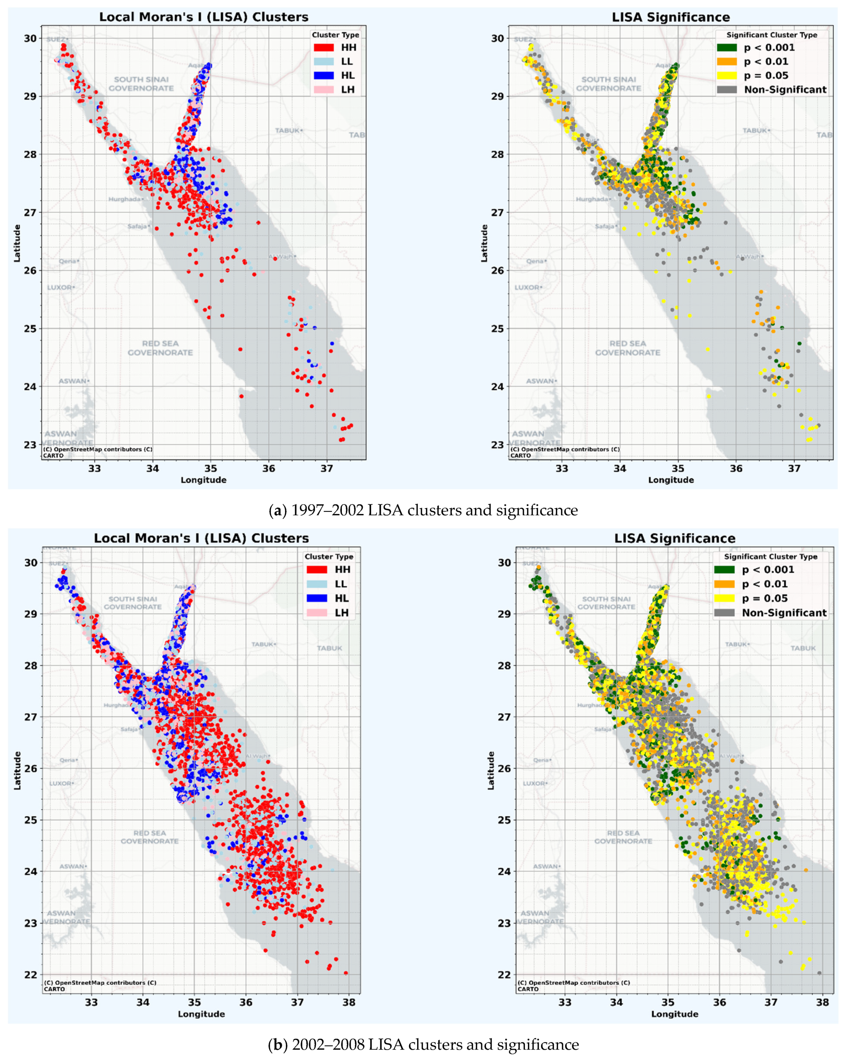
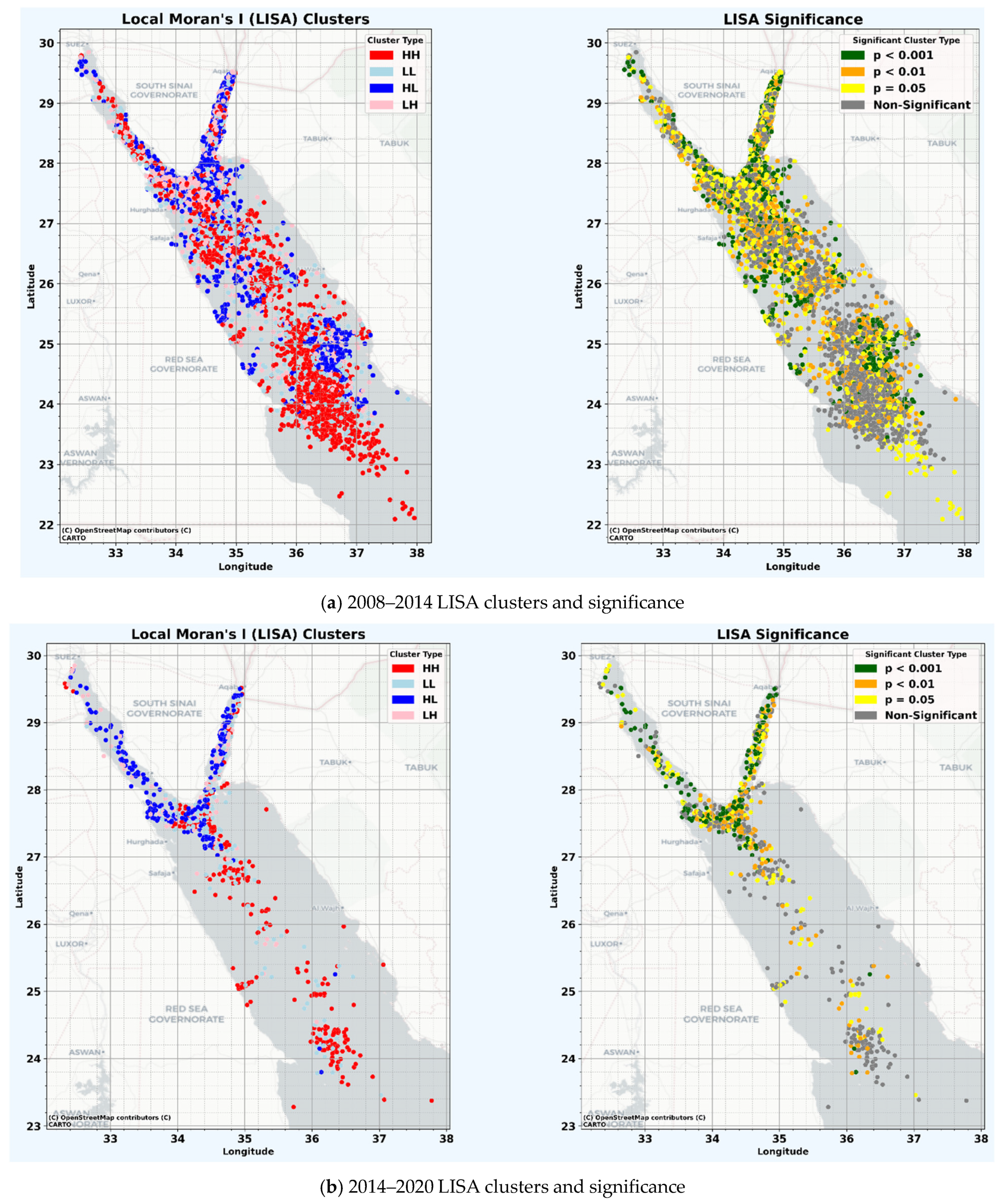
5.3.4. Local Moran’s I (LMI)

Local Moran’s Index (LMI) was utilized to uncover and interpret local autocorrelation patterns in seismic activity [61]. This analysis is crucial for identifying spatial patterns not evident in global measures, revealing clusters, outliers, and local spatial dependencies and heterogeneities [43]. The comprehensive LMI results presented in Table 4 provide a thorough analysis of spatial clustering and autocorrelation in seismic events, highlighting regions that may be influenced by seismotectonic activities. Incorporating Z-scores and p-values into LMI calculations enhances the precision in identifying seismic activities deviating from random patterns.
In Table 6, the LMI analysis, categorizing seismic events in the Red Sea area by magnitude range, reveals significant spatial autocorrelation. The LMI Index values, across magnitudes ranging from 1.00 to 3.20, consistently indicate clustering, evidenced by positive values. For the 1.00–1.55 magnitude range, an LMI Index of 0.123003, a low but significant Z-score of 0.224410, and a p-value of 0.005188 suggest modest clustering, reflective of minor fault activities or stress adjustments in the crust. As magnitudes increase, the LMI Index slightly decreases, with the 1.55–2.10 range showing 0.090980, indicating a dispersed clustering pattern, potentially due to varying geological processes. The 2.10–2.65 range’s further reduced LMI Index of 0.029216, alongside a Z-score of 0.063909 and a significant p-value of 0.001094, still indicates notable clustering but less intense than lower magnitudes, suggesting concentrated seismic activity aligning with major fault lines or tectonic stress zones. In the highest range, 2.65–3.20, the LMI Index increases to 0.062832, with a Z-score of 0.083825 and a p-value of 0.006475, denoting more pronounced clustering for higher magnitudes, possibly influenced by major tectonic features. Overall, the LMI analysis reveals a complex relationship between the magnitude and spatial clustering of seismic events in the Red Sea area. It highlights seismicity patterns that are intricately linked to the region’s seismotectonic framework. The observed clustering suggests concentrated distributions of stress and strain, indicating that seismic activity is not random but rather concentrated in specific areas. These areas likely correspond to key geological structures like faults and rifts, underscoring the importance of this analysis in understanding and predicting seismic behavior in tectonically active regions [5,8,58].

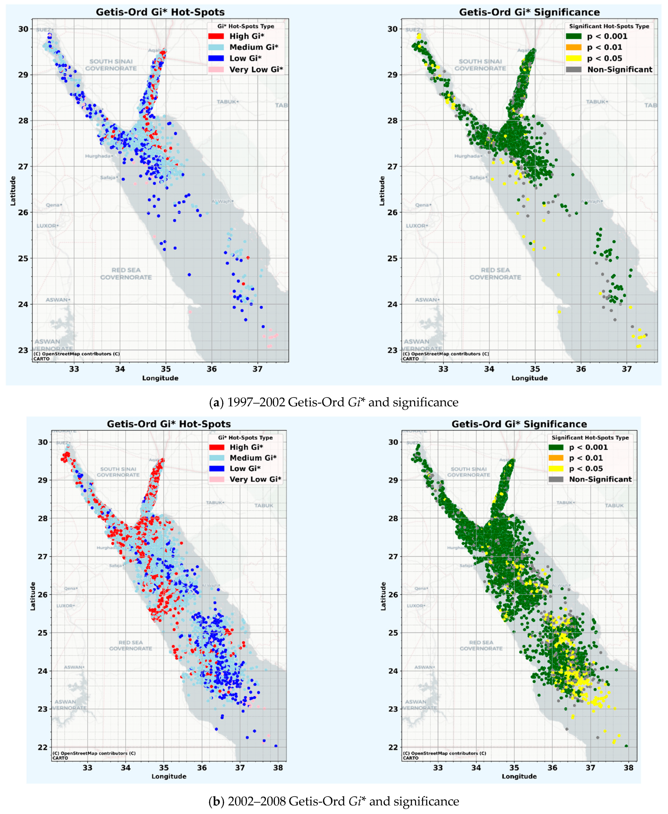
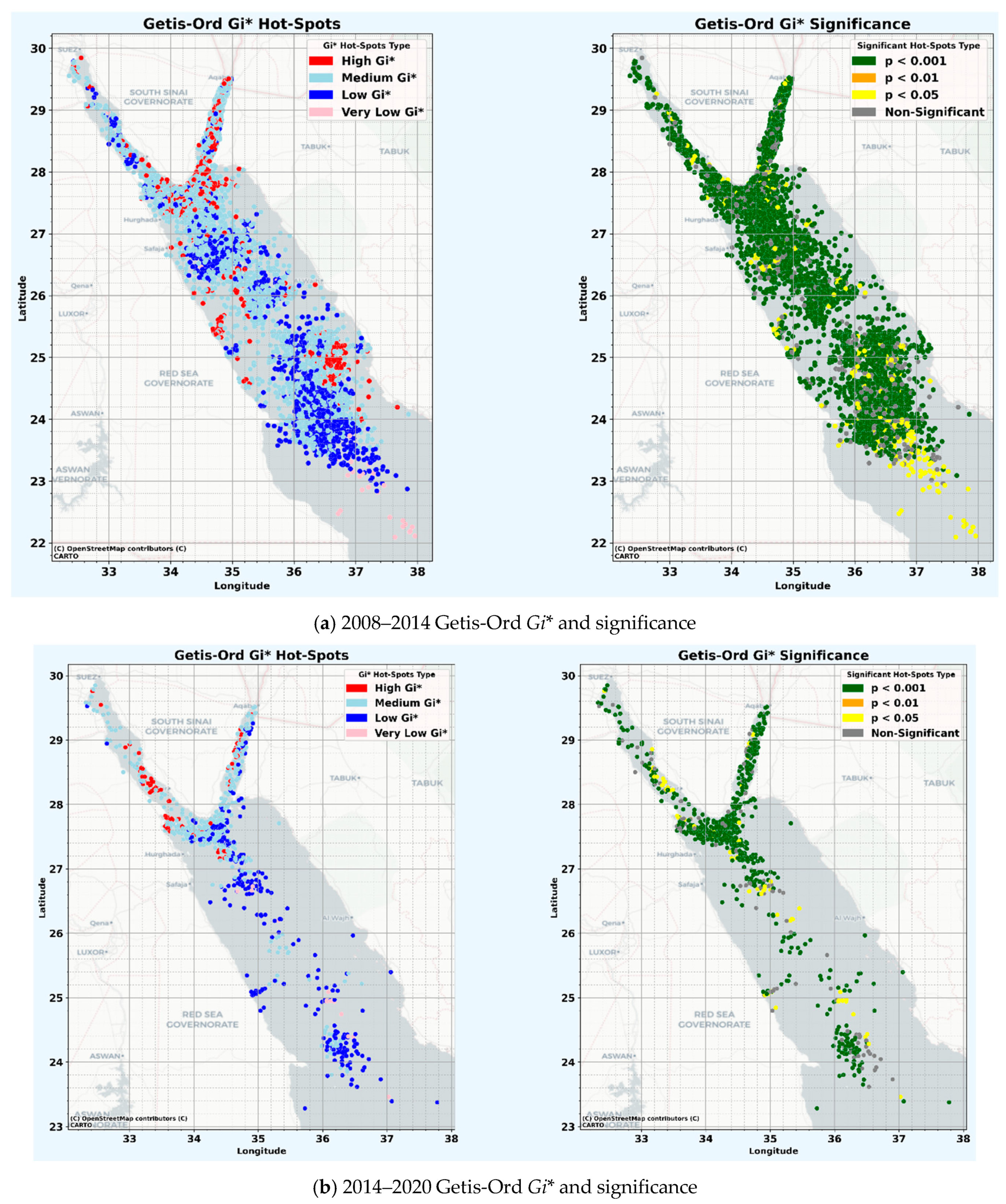
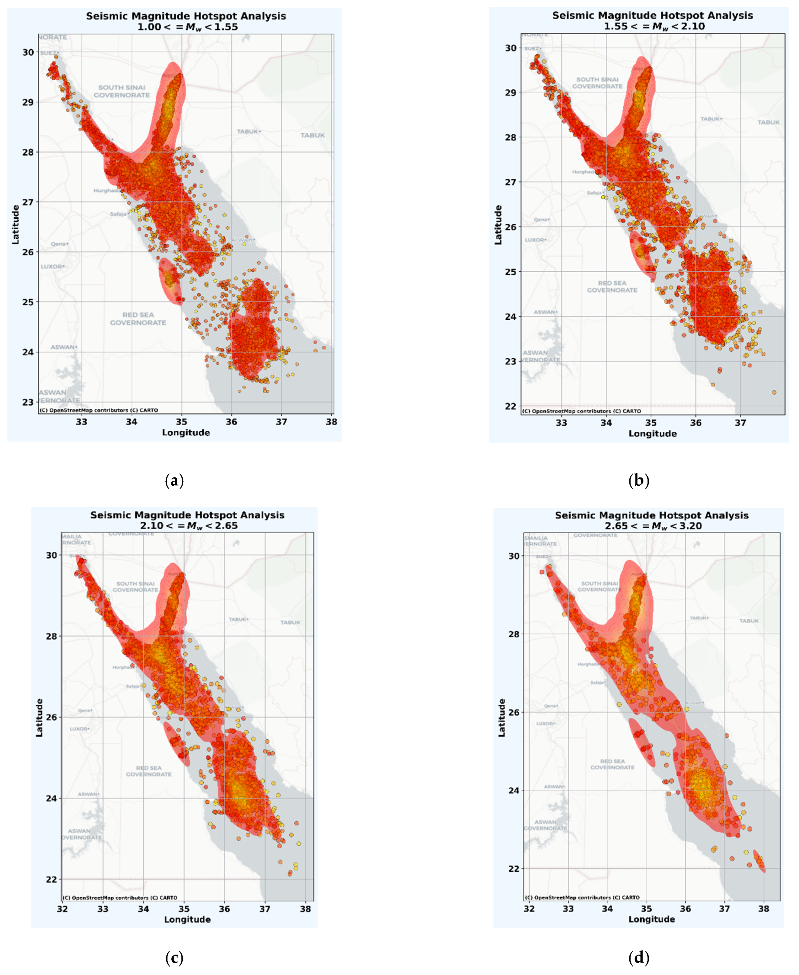
5.3.5. Local Variations and Concentrated Areas in Seismic Activity

The geostatistical characterization of seismic activity in the Red Sea region has been augmented through the integration of univariate Local Indicators of Spatial Association (LISA) [44] and Getis-Ord Gi* [62,63] statistics. This method offers a thorough insight into localized variations and clusters, enabling the identification of concentrated areas with heightened seismic activity.
An analysis of Local Indicators of Spatial Association (LISA) maps was performed to identify clusters and statistically significant seismicity data. The goal was to generate cluster maps using spatial autocorrelation data, as described in Anselin’s 2009 work on OpenGeoDa [64]. This analysis aimed to pinpoint spatial patterns of earthquake events, including earthquake clusters, as well as to understand the spatiotemporal dynamics, mechanisms, and characteristics of seismic activity. Figure 7 and Figure 8 display the outcomes of a Local Indicators of Spatial Association (LISA) analysis, examining seismic events in the Red Sea region over four distinct time frames: 1997–2002 (Figure 7a), 2002–2008 (Figure 7b), 2008–2014 (Figure 8a), and 2014–2020 (Figure 8b). This analysis categorizes earthquake events into distinct clusters based on their spatial correlations and magnitudes. This temporal segmentation facilitates the examination of evolving or consistent seismic patterns. The analysis categorizes seismic spatial patterns into four clusters: high-high (HH), indicating regions of frequent, intense seismic activity; low-low (LL), denoting areas with minimal seismic events; and two types of spatial outliers, high-low (HL) and low-high (LH), which identify areas where seismic magnitudes significantly diverge from their immediate environments. HH clusters suggest seismicity clustering, potentially linked to active tectonic features, while LL clusters imply areas of relative tectonic inactivity. The HL and LH outliers may signal localized geophysical anomalies or tectonic complexities, where observed seismic activities markedly differ from those of surrounding areas.
Adjacent to these cluster maps, the figures also illustrate the statistical significance of the identified clusters, employing p-value thresholds to challenge the hypothesis of random spatial distribution. Clusters with significant p-values, especially along the central axis of the Red Sea, highlight a spatially correlated pattern that could be connected to the region’s tectonic structure. Conversely, clusters lacking statistical significance might represent either random distributions or an insufficiency of data to establish a discernible pattern.
The aggregation of significant clusters along the Red Sea’s central axis is particularly salient, possibly indicating a correlation with the seafloor spreading center and related earthquake activities. Non-significant clusters, though less conclusive, may still hold interest as they could represent areas of more random seismic activity or locations with inadequate data to confirm spatial patterns.
Overall, the analysis reveals both concentrated and isolated seismic events in the Red Sea region, with varying degrees of statistical significance suggesting a complex seismic structure; some areas, especially along the central axis, have consistently exhibited high seismicity over the examined periods. The persistence of HH clusters could imply ongoing tectonic activities, such as rifting, that continuously produce earthquakes. Additionally, the presence of significant HL outliers highlights potential unforeseen seismic hazards in typically quiescent areas, necessitating further research for comprehensive risk assessment.
The Getis-Ord Gi* statistic, on the other hand, is used to identify ’hot spots’ and ’cold spots’ of seismic activity in the mapped area. It is more about the intensity or concentration of earthquake magnitudes in a geographical space of the area. Figure 9 and Figure 10 show the results from the Getis-Ord Gi* analysis, which investigates seismic activities in the Red Sea area across four separate time periods: from 1997 to 2002 (illustrated in Figure 9a), 2002 to 2008 (Figure 9b), 2008 to 2014 (Figure 10a), and 2014 to 2020 (Figure 10b).
The Getis-Ord Gi* method computes a Z-score for each earthquake’s magnitude, signifying the extent of spatial clustering of either high or low magnitude values. This approach evaluates the magnitude of an individual earthquake and its neighboring events, contrasting this localized aggregate with the total sum of magnitudes across the region. This comparison yields an understanding of the concentration levels of either high or low magnitude values in specific areas. Consequently, regions with elevated Z-scores are classified as hotspots, indicating that the observed earthquake magnitude is significantly above the average. Conversely, areas with diminished Z-scores are identified as coldspots, signifying that the magnitude is below average.
Figure 9a illustrates the Getis-Ord Gi* clustering analysis for Red Sea earthquakes between 1997 and 2002, pinpointing areas with diverse intensities of seismic activity. The spatial distribution map categorizes regions into high Gi* to signify prominent earthquake clustering and then into zones of progressively decreasing activity. Additionally, the Gi* significance map portrays the statistical significance of these concentrated or dissipated seismic activity areas. This analysis accentuates areas with heightened seismic activity, especially along the rift axis where the African and Arabian plates diverge, indicating a robust link with tectonic movements. Expanding on this, Figure 9b continues the analysis for the period from 2002 to 2008. Both the concentrated areas map and the significance map in this figure delineate the spatial intensity or clustering and statistical significance of seismic activities. Notably, high Gi* values or clustered seismicity are primarily located along the central axis of the Red Sea, marking the divergent boundary and underscoring areas of intense seismic activity. In contrast, the peripheral areas, designated as low Gi* and very low Gi*, correspond to more stable parts of the oceanic crust. The significance map’s corroboration of these clusters underlines their non-random distribution, with a strong association to the tectonic dynamics at the Red Sea’s spreading center. This concurrence underscores the efficacy of the Getis-Ord Gi* method in discerning seismic patterns in direct relation to tectonic processes.
Figure 10a,b present the Getis-Ord Gi* statistic maps for the 2008–2014 and 2014–2020 periods, respectively, in the Red Sea region. These maps visually represent seismic activity, with hotspots in various shades of red and coldspots in shades of blue, delineating a spectrum of earthquake activity from high Gi* to very low Gi*. Accompanying these are the Gi* significance maps, which use a color gradient from dark green to yellow to indicate the statistical significance of these seismic patterns, thereby identifying areas where seismic clustering is not random. The distribution of high Gi* hotspots, predominantly along the Red Sea’s axial trough, is consistent with the region’s tectonic activity. This zone is an area of active rifting between the African and Arabian plates, characterized by seismic events associated with the formation of new oceanic crust and extensional tectonics. The concentration of seismic hotspots along this tectonic boundary points to their strong association with primary rifting processes, including seafloor spreading, faulting, and magmatic activity. In contrast, areas marked as low Gi* and very low Gi* are typically found on the flanks of the rift, indicating regions that are more stable and less affected by tectonic activity. The Gi* significance maps lend statistical credibility to these observations, affirming the spatial distribution of seismic hotspots and their significant alignment with the tectonic structure of the Red Sea rift system. These findings underscore the profound connection between seismic events and tectonic mechanisms in the Red Sea, exemplifying an active divergent plate boundary.
Upon meticulous analysis of the results presented in Figure 7, Figure 8, Figure 9 and Figure 10, a discernible systematic variation within a 26.7 to 27.7 latitude range was observed. This variation can be attributed to a confluence of factors. Primarily, it emerges from the differential seismicity reported across each distinct time period under consideration. These discrete temporal intervals exhibit unique patterns of seismic activity, significantly contributing to the variations observed. Additionally, the statistical framework underpinning the Local Indicators of Spatial Autocorrelation (LISA) method must be acknowledged. The method’s statistical nature, as rigorously outlined in the significance figures for each period in each respective graph, plays an integral role in shaping these variations. The LISA methodology, with its focus on spatial autocorrelation, adeptly identifies regions characterized by significant spatial clustering or dispersion of seismic events. These variations are reflective of the intricate and dynamic interplay of spatial patterns in seismic activity across different time frames. These variations reflect the complex interplay of spatial patterns in seismic activity over time.
A Kernel Density Estimator (KDE) [48,65] is a robust statistical method for analyzing the spatial intensity of seismic events. This assists in identifying areas with higher earthquake frequencies, known as hotspots or local clusters. Figure 11 displays a series of KDE-derived clustered patterns, each corresponding to a different moment magnitude ( M w ) range. Figure 11a–d present a sequential spatial analysis of seismic activity in the Red Sea region across increasing moment magnitude ranges. Starting from  1.00 M w < 1.55  in Figure 11a, the activity is primarily concentrated in the Gulf of Aqaba and Northern Red Sea, highlighting areas of potential tectonic or volcanic significance. This pattern persists and intensifies in the  1.55 M w < 2.10  range (Figure 11b), with notable clusters also in the southern Gulf of Suez. As the magnitude range extends to  2.10 M w < 2.65  in Figure 11c, and further to  2.65 M w < 3.20  in Figure 11d, the seismicity demonstrates a more focused pattern. The density and spatial distribution of events increase, especially in the central part of the Red Sea, indicating a higher potential for accumulating and releasing significant seismic energy. This trend suggests that larger events are concentrated in areas with heightened tectonic stress, aligning with the region’s geotectonic dynamics and marking them as zones of pronounced seismic activity. There is a noticeable shift from widespread distribution of lower magnitude events (see Figure 11a) to a more concentrated pattern of higher magnitude events (see Figure 11d). This transition suggests zones of higher stress accumulation within the Earth’s crust, particularly in the Central Red Sea. These areas emerge as having key concentrated seismic activity with an elevated likelihood of experiencing substantial seismic events. KDE visualizations are crucial for seismic hazard assessment, indicating that while lower magnitude events are common and dispersed, the potential for damage escalates with higher magnitude events concentrated in active tectonic zones. This gradient in seismicity underscores the need for differentiated disaster preparedness and infrastructure resilience strategies across the region [17].

6. Conclusions

This study has conducted an in-depth geostatistical analysis of seismic activity in the Red Sea region, covering the period from 1997 to 2020. Utilizing a GIS framework and a suite of spatial analytic methods—including ANN, QCA, Global Moran’s I, Local Moran’s I, and the Getis-Ord Gi* statistic—we have effectively unraveled the complex temporal and spatial dynamics of seismic events in this tectonically active area. Our findings have outlined distinct seismic patterns along the Central Red Sea axis, which are indicative of the rifting dynamics between the African and Arabian plates.
The application of ANN and QCA has shed light on the general distribution and density of seismic occurrences, while GMI and LMI have been instrumental in highlighting areas of spatial clustering and dispersion. Notably, LMI has revealed significant clustering of seismic activities across different magnitudes, suggesting a nuanced relationship between earthquake magnitudes and the region’s dynamic tectonic setting.
Through LISA analysis for various periods, we have demonstrated consistent spatial autocorrelation in seismic activities. The identification of high-high clusters along the central rift axis underscores zones of elevated seismicity, while low-low clusters indicate areas of relative tectonic stability. These findings, corroborated by LISA significance maps, align well with the known tectonic divergence in the Red Sea.
Moreover, the analysis of Getis-Ord Gi* statistic maps has confirmed persistent seismic clustering along the central rift, indicative of active tectonic rifting. The temporal consistency of these patterns underscores the ongoing nature of the rifting process, which is integral to the formation of new oceanic crust in the Red Sea.
Kernel Density Estimator analyses across various moment magnitude ranges have revealed concentrations of seismic activity in key areas such as the Gulfs of Aqaba and Suez, as well as the Central and Northern Red Sea. This spatial distribution correlates with known geological features and fault lines. Importantly, higher magnitude events tend to localize in areas of greater tectonic stress, highlighting the complex interplay between seismic events and the underlying geological framework. Our comprehensive analysis revealed pronounced seismic patterns along the Central Red Sea axis, correlating with tectonic rifting between the African and Arabian plates. The spatial analysis techniques employed delineated areas of heightened seismic activity and zones of relative tectonic stability. Notably, the Local Moran’s I highlighted significant clustering of seismic activities, with variations in intensity across magnitudes. The Getis-Ord Gi* statistic maps confirmed persistent seismic hotspots along the central rift, indicative of active tectonic processes. Kernel Density Estimator analyses revealed a concentration of seismic activity in key geological areas, with higher magnitude events localizing in regions of greater tectonic stress. These findings underscore the dynamic tectonic setting of the Red Sea and demonstrate the utility of geostatistical techniques in seismic analysis.

Author Contributions

Conceptualization, methodology, software development, validation, data collection, analysis and writing: S.S.R.M.; Conceptualization, review and editing: M.H.Y. and M.M.; Data collection, analysis A.M.F. and B.E. All authors have read and agreed to the published version of the manuscript.

Funding

This reaserch was funded by the Deputyship for Research and Innovation, “Ministry of Education” in Saudi Arabia (IFKSUOR3-093-2).

Institutional Review Board Statement

Not applicable.

Informed Consent Statement

Not applicable.

Data Availability Statement

The data presented in this study are available upon reasonable request from the first author. The data are not publicly available due to official regulations.

Acknowledgments

The authors would like to express their sincere gratitude to the Egyptian National Seismic Network (ENSN) at the National Research Institute of Astronomy and Geophysics (NRIAG) for their invaluable assistance with this research. The authors wish to express their gratitude to the Deputyship for Research and Innovation, “Ministry of Education” in Saudi Arabia for funding this research (IFKSUOR3-093-2).

Conflicts of Interest

The authors declare no conflicts of interest.

References

  1. Carvalho, S.; Kürten, B.; Krokos, G.; Hoteit, I.; Ellis, J. The Red Sea. In World Seas: An Environmental Evaluation; Elsevier: Amsterdam, The Netherlands, 2019; pp. 49–74. [Google Scholar]
  2. Luo, P.; Sun, Y.; Wang, S.; Wang, S.; Lyu, J.; Zhou, M.; Nakagami, K.; Takara, K.; Nover, D. Historical Assessment and Future Sustainability Challenges of Egyptian Water Resources Management. J. Clean. Prod. 2020, 263, 121154. [Google Scholar] [CrossRef]
  3. Gladstone, W.; Curley, B.; Shokri, M.R. Environmental Impacts of Tourism in the Gulf and the Red Sea. Mar. Pollut. Bull. 2013, 72, 375–388. [Google Scholar] [CrossRef] [PubMed]
  4. Augustin, N.; van der Zwan, F.M.; Devey, C.W.; Ligi, M.; Kwasnitschka, T.; Feldens, P.; Bantan, R.A.; Basaham, A.S. Geomorphology of the Central Red Sea Rift: Determining Spreading Processes. Geomorphology 2016, 274, 162–179. [Google Scholar] [CrossRef]
  5. Amjadi, A.; Akashe, B.; Ariamanesh, M.; Pourkermani, M. The Comparison of the Divergent and Convergent Tectonic Plates Margins Seismicity-the Case Study: Red Sea and Zagros. Contrib. Geophys. Geod. 2020, 50, 261–285. [Google Scholar] [CrossRef]
  6. Bosworth, W.; Huchon, P.; McClay, K. The Red Sea and Gulf of Aden Basins. J. Afr. Earth Sci. 2005, 43, 334–378. [Google Scholar] [CrossRef]
  7. Ambraseys, N.N.; Melville, C.P.; Adams, R.D. The Seismicity of Egypt, Arabia and the Red Sea: A Historical Review; Cambridge University Press: Cambridge, UK, 2005. [Google Scholar]
  8. El-Isa, Z. Seismicity and Seismotectonics of the Red Sea Region. Arab. J. Geosci. 2015, 8, 8505–8525. [Google Scholar] [CrossRef]
  9. Moustafa, S.S.; Al-Arifi, N.S.; Jafri, M.K.; Naeem, M.; Alawadi, E.A.; Metwaly, M.A. First Level Seismic Microzonation Map of Al-Madinah Province, Western Saudi Arabia Using the Geographic Information System Approach. Environ. Earth Sci. 2016, 75, 251. [Google Scholar] [CrossRef]
  10. Aldamegh, K.S.; Hussein Moussa, H.; Al-Arifi, S.N.; Moustafa, S.S.; Moustafa, M.H. Focal Mechanism of Badr Earthquake, Saudia Arabia of 27 August 2009. Arab. J. Geosci. 2012, 5, 599–606. [Google Scholar] [CrossRef]
  11. Al-Amri, A.; Punsalan, B.; Uy, E. Spatial Distribution of the Seismicity Parameters in the Red Sea Regions. J. Asian Earth Sci. 1998, 16, 557–563. [Google Scholar] [CrossRef]
  12. Hagos, L.; Arvidsson, R.; Roberts, R. Application of the Spatially Smoothed Seismicity and Monte Carlo Methods to Estimate the Seismic Hazard of Eritrea and the Surrounding Region. Nat. Hazards 2006, 39, 395–418. [Google Scholar] [CrossRef]
  13. Abdalzaher, M.S.; El-Hadidy, M.; Gaber, H.; Badawy, A. Seismic Hazard Maps of Egypt Based on Spatially Smoothed Seismicity Model and Recent Seismotectonic Models. J. Afr. Earth Sci. 2020, 170, 103894. [Google Scholar] [CrossRef]
  14. Al-Ahmadi, K.; Al-Amri, A.; See, L. A Spatial Statistical Analysis of the Occurrence of Earthquakes Along the Red Sea Floor Spreading: Clusters of Seismicity. Arab. J. Geosci. 2014, 7, 2893–2904. [Google Scholar] [CrossRef]
  15. Moustafa, S.S.; Abdalzaher, M.S.; Abdelhafiez, H. Seismo-Lineaments in Egypt: Analysis and Implications for Active Tectonic Structures and Earthquake Magnitudes. Remote Sens. 2022, 14, 6151. [Google Scholar] [CrossRef]
  16. Asim, K.M.; Moustafa, S.S.; Niaz, I.A.; Elawadi, E.A.; Iqbal, T.; Martínez-Álvarez, F. Seismicity Analysis and Machine Learning Models for Short-Term Low Magnitude Seismic Activity Predictions in Cyprus. Soil Dyn. Earthq. Eng. 2020, 130, 105932. [Google Scholar] [CrossRef]
  17. Moustafa, S.S.; Abdalzaher, M.S.; Naeem, M.; Fouda, M.M. Seismic Hazard and Site Suitability Evaluation Based on Multicriteria Decision Analysis. IEEE Access 2022, 10, 69511–69530. [Google Scholar] [CrossRef]
  18. Bansal, P.; Ardell, A.J. Average Nearest-Neighbor Distances Between Uniformly Distributed Finite Particles. Metallography 1972, 5, 97–111. [Google Scholar] [CrossRef]
  19. Diggle, P.J.; Milne, R.K. Negative Binomial Quadrat Counts and Point Processes. Scand. J. Stat. 1983, 16, 257–267. [Google Scholar]
  20. Westerholt, R. A Simulation Study to Explore Inference about Global Moran’s i with Random Spatial Indexes. Geogr. Anal. 2023, 55, 621–650. [Google Scholar] [CrossRef]
  21. Ghebreab, W. Tectonics of the Red Sea Region Reassessed. Earth-Sci. Rev. 1998, 45, 1–44. [Google Scholar] [CrossRef]
  22. Al-Amri, A.; Punsalan, B.; Khalil, A.; Uy, E.; Center, S.S. Seismic Hazard Assessment of Western Saudi Arabia and the Red Sea Region. Bull. Inter. Inst. Seismol. Earth Eng. Jpn. Spec. Ed. 2003, special eddition, 95–112. [Google Scholar]
  23. Daggett, P.H.; Morgan, P.; Boulos, F.; Hennin, S.; El-Sherif, A.; El-Sayed, A.; Basta, N.; Melek, Y. Seismicity and Active Tectonics of the Egyptian Red Sea Margin and the Northern Red Sea. Tectonophysics 1986, 125, 313–324. [Google Scholar] [CrossRef]
  24. Bosworth, W.; Taviani, M.; Rasul, N.M. Neotectonics of the Red Sea, Gulf of Suez and Gulf of Aqaba. In Geological Setting, Palaeoenvironment and Archaeology of the Red Sea; Springer: Berlin/Heidelberg, Germany, 2019; pp. 11–35. [Google Scholar]
  25. Deif, A.; Hamed, H.; Ibrahim, H.; Elenean, K.A.; El-Amin, E. Seismic Hazard Assessment in Aswan, Egypt. J. Geophys. Eng. 2011, 8, 531–548. [Google Scholar] [CrossRef]
  26. Garfunkel, Z.; Zvi, B.-A.; Elisa, K. Dead Sea Transform Fault System: Reviews; Springer: Berlin/Heidelberg, Germany, 2014. [Google Scholar]
  27. Badawy, A. Seismicity and Kinematic Evolution of the Sinai Plate. Ph.D. Thesis, Eötvös University, Budapest, Hungary, 1996. [Google Scholar]
  28. Badawy, A.; Horváth, F. Seismicity of the Sinai Subplate Region: Kinematic Implications. J. Geodyn. 1999, 27, 451–468. [Google Scholar] [CrossRef]
  29. Armaş, I. Multi-Criteria Vulnerability Analysis to Earthquake Hazard of Bucharest, Romania. Nat. Hazards 2012, 63, 1129–1156. [Google Scholar] [CrossRef]
  30. Sofyan, H.; Rahayu, L.; Lusiani, E. Spatial Autocorrelation of Earthquake Magnitudes in Tripa Fault, Aceh Province, Indonesia. In IOP Conference Series Earth and Environmental Science; IOP Publishing: Bristol, UK, 2019; Volume 273, p. 012048. [Google Scholar]
  31. Cao, Z.; Zhang, H.; Liu, Y.; Liu, S.; Feng, L.; Yin, L.; Zheng, W. Spatial Distribution Analysis of Seismic Activity Based on GMI, LMI, and LISA in China. Open Geosci. 2022, 14, 89–97. [Google Scholar] [CrossRef]
  32. Khan, M.J. Modelling of Seismicity in Southern Pakistan Using GIS Techniques. Earth Sci. Inform. 2020, 13, 1327–1340. [Google Scholar] [CrossRef]
  33. Fischer, M.M.; Getis, A. Handbook of Applied Spatial Analysis: Software Tools, Methods and Applications; Springer: Berlin/Heidelberg, Germany, 2010. [Google Scholar]
  34. Affan, M.; Syukri, M.; Wahyuna, L.; Sofyan, H. Spatial Statistic Analysis of Earthquakes in Aceh Province Year 1921–2014: Cluster Seismicity. Aceh Int. J. Sci. Technol. 2016, 5, 54–62. [Google Scholar] [CrossRef]
  35. Moustafa, S.S.; Mohamed, G.-E.A.; Metwaly, M. Production of a Homogeneous Seismic Catalog Based on Machine Learning for Northeast Egypt. Open Geosci. 2021, 13, 1084–1104. [Google Scholar] [CrossRef]
  36. Friedman, J.H.; Baskett, F.; Shustek, L.J. An Algorithm for Finding Nearest Neighbors. IEEE Trans. Comput. 1975, 100, 1000–1006. [Google Scholar] [CrossRef]
  37. Adams, W.M. Application of The Variance-To-Mean Ratio Method for Determining Neutron Multiplication Parameters of Critical and Subcritical Reactors (Reactor Noise, Feynman-Alpha); The University of Arizona: Tucson, AZ, USA, 1985. [Google Scholar]
  38. Mare, D.S.; Moreira, F.; Rossi, R. Nonstationary z-Score Measures. Eur. J. Oper. Res. 2017, 260, 348–358. [Google Scholar] [CrossRef]
  39. Scott, L.M.; Janikas, M.V. Spatial Statistics in ArcGIS. In Handbook of Applied Spatial Analysis: Software Tools, Methods and Applications; Springer: Berlin/Heidelberg, Germany, 2009; pp. 27–41. [Google Scholar]
  40. Fu, W.J.; Jiang, P.K.; Zhou, G.M.; Zhao, K.L. Using Moran’s i and GIS to Study the Spatial Pattern of Forest Litter Carbon Density in a Subtropical Region of Southeastern China. Biogeosciences 2014, 11, 2401–2409. [Google Scholar] [CrossRef]
  41. Getis, A.; Aldstadt, J. Constructing the Spatial Weights Matrix Using a Local Statistic. Geogr. Anal. 2004, 36, 90–104. [Google Scholar] [CrossRef]
  42. Rogerson, P.A.; Kedron, P. Optimal Weights for Focused Tests of Clustering Using the Local Moran Statistic. Geogr. Anal. 2012, 44, 121–133. [Google Scholar] [CrossRef]
  43. Tiefelsdorf, M.; Boots, B. A Note on the Extremities of Local Moran’s Iis and Their Impact on Global Moran’s i. Geogr. Anal. 1997, 29, 248–257. [Google Scholar] [CrossRef]
  44. Anselin, L. Local Indicators of Spatial Association—LISA. Geogr. Anal. 1995, 27, 93–115. [Google Scholar] [CrossRef]
  45. Manepalli, U.; Bham, G.H.; Kandada, S. Evaluation of Hotspots Identification Using Kernel Density Estimation (k) and Getis-Ord (Gi*) on i-630. In Proceedings of the 3rd International Conference on Road Safety and Simulation, Indianapolis, IN, USA, 14–15 September 2011; National Academy of Sciences: Washington, DC, USA, 2011; Volume 21, pp. 14–16. [Google Scholar]
  46. Songchitruksa, P.; Zeng, X. Getis–Ord Spatial Statistics to Identify Hot Spots by Using Incident Management Data. Transp. Res. Rec. 2010, 2165, 42–51. [Google Scholar] [CrossRef]
  47. Chen, Y.-C. A Tutorial on Kernel Density Estimation and Recent Advances. Biostat. Epidemiol. 2017, 1, 161–187. [Google Scholar] [CrossRef]
  48. Węglarczyk, S. Kernel Density Estimation and Its Application. In ITM Web of Conferences; EDP Sciences: Les Ulis, France, 2018; Volume 23, p. 00037. [Google Scholar]
  49. Flahaut, B.; Mouchart, M.; San Martin, E.; Thomas, I. The Local Spatial Autocorrelation and the Kernel Method for Identifying Black Zones: A Comparative Approach. Accid. Anal. Prev. 2003, 35, 991–1004. [Google Scholar] [CrossRef] [PubMed]
  50. Soliman, M.S.; Zahran, H.M.; Elhadidy, S.Y.; Alraddadi, W.W. Evaluation of Saudi National Seismic Network (SNSN) Detectability. Arab. J. Geosci. 2019, 12, 330. [Google Scholar] [CrossRef]
  51. Fergany, E.; Omar, K.; Mohammed, G.-E.-K.A. Evolution in Seismic Monitoring System and Updating Seismic Zones of Egypt. NRIAG J. Astron. Geophys. 2020, 9, 548–557. [Google Scholar] [CrossRef]
  52. Wiemer, S. A Software Package to Analyze Seismicity: ZMAP. Seismol. Res. Lett. 2001, 72, 373–382. [Google Scholar] [CrossRef]
  53. Shiffler, R.E. Maximum z Scores and Outliers. Am. Stat. 1988, 42, 79–80. [Google Scholar]
  54. Babiker, N.; Mula, A.; El-Hadidy, S. A Unified Mw-Based Earthquake Catalogue and Seismic Source Zones for the Red Sea Region. J. Afr. Earth Sci. 2015, 109, 168–176. [Google Scholar] [CrossRef]
  55. Moustafa, S.S.R. Application of the Analytic Hierarchy Process for Evaluating Geo-Hazards in the Greater Cairo Area, Egypt. Electron. J. Geotech. Eng. 2015, 20, 1921–1938. [Google Scholar]
  56. Mitchell, N.C.; Stewart, I.C. The Modest Seismicity of the Northern Red Sea Rift. Geophys. J. Int. 2018, 214, 1507–1523. [Google Scholar] [CrossRef]
  57. Ruch, J.; Keir, D.; Passarelli, L.; Di Giacomo, D.; Ogubazghi, G.; Jonsson, S. Revealing 60 Years of Earthquake Swarms in the Southern Red Sea, Afar and the Gulf of Aden. Front. Earth Sci. 2021, 9, 664673. [Google Scholar] [CrossRef]
  58. Johnson, P. Tectonic Map of Saudi Arabia and Adjacent Areas, Ministry of Petroleum and Mineral Resources, Deputy Ministry Mineral; Resources Technical Report USGS-TR-98-3; Ministry of Petroleum and Mineral Resources: Jeddah, Saudi Arabia, 1998.
  59. Mitchell, A. The ESRI Guide to GIS Analysis: Geographic Patterns and Relationships. Redlands: ESRI; ESRI, Inc.: Redlands, CA, USA, 1999; Volume 1. [Google Scholar]
  60. Aslam, B.; Naseer, F. A Statistical Analysis of the Spatial Existence of Earthquakes in Balochistan: Clusters of Seismicity. Environ. Earth Sci. 2020, 79, 41. [Google Scholar] [CrossRef]
  61. Anselin, L. The Moran Scatterplot as an ESDA Tool to Assess Local Instability in Spatial Association. In Spatial Analytical Perspectives on GIS; Routledge: London, UK, 2019; pp. 111–126. [Google Scholar]
  62. Ord, J.K.; Getis, A. Local Spatial Autocorrelation Statistics: Distributional Issues and an Application. Geogr. Anal. 1995, 27, 286–306. [Google Scholar] [CrossRef]
  63. Getis, A. Spatial Statistics. Geogr. Inf. Syst. 1999, 1, 239–251. [Google Scholar]
  64. Anselin, L.; McCann, M. OpenGeoDa, Open Source Software for the Exploration and Visualization of Geospatial Data. In Proceedings of the 17th ACM SIGSPATIAL International Conference on Advances in Geographic Information Systems, New York, NY, USA, 4–6 November 2009; pp. 550–551. [Google Scholar]
  65. Dehnad, K. Density Estimation for Statistics and Data Analysis 1987. Technometrics 1987, 29, 495. [Google Scholar] [CrossRef]
Figure 1. (a) Principal geological and tectonic characteristics of the Red Sea region, including the extensional ridges and oceanic troughs, as well as the adjacent elevated peripheries of the Arabian and Nubian Shield, accompanied by the dispersion of Late Cenozoic volcanic terrains, commonly known as harrats (adapted from [24]). (b) Spatial distribution of documented historical and instrumentally recorded seismic occurrences within the vicinity of the Red Sea (adapted from [25]).
Applsci 14 01455 g001
Figure 2. (a) Spatial configuration of seismic stations operated by the Saudi Geological Survey (SGS) [50]. (b) Spatial distribution of collected earthquake events captured by the Saudi National Seismic Network (SNSN). (c) Network topology of seismic stations in the Egyptian National Seismic Network (ENSN) [51]. (d) Geospatial variability in earthquake events recorded and collected by the Egyptian National Seismic Network (ENSN).
Applsci 14 01455 g002
Figure 3. Selected seismic data: a compilation of key earthquake parameters from the ENSN and SNSN datasets, highlighting spatial coordinates, and depth variations for the period 1997–2020.
Applsci 14 01455 g003
Figure 4. Temporal distribution of earthquakes in the Red Sea across different time scales. Each subplot illustrates the frequency of earthquakes over a specific period: (a) daily, (b) weekly, (c) monthly, and (d) yearly. Horizontal dashed lines in each subplot indicate the minimum (red), maximum (green), and mean (blue) counts for that time scale.
Applsci 14 01455 g004aApplsci 14 01455 g004b
Figure 5. Multifaceted analysis of spatial earthquake distribution characteristics in the Red Sea: (a,c) showing the distribution of earthquake magnitudes across latitudinal and longitudinal ranges. (b,d) depicting the depth distribution of earthquakes along latitudinal and longitudinal coordinates. (e) A 3D histogram illustrating the frequency of earthquakes across varying magnitudes and depths.
Applsci 14 01455 g005
Figure 6. Global Moran’s I (GMI) scatter plots depicting spatial autocorrelation across distinct earthquake magnitude ranges. Each plot is partitioned into quadrants by blue dashed lines, representing the respective means of magnitude and spatial lag of magnitude. Red line represents the fitting of a regression between magnitude and the spatial lag of magnitude. This regression fitting is crucial for illustrating the relationship between the magnitude of seismic events and their corresponding spatial lags. By doing so, it allows us to understand how the magnitude of a seismic event correlates with the magnitudes of events in its proximity, providing valuable insights into the spatial distribution of seismic intensity.
Applsci 14 01455 g006
Figure 7. Spatial distribution of Local Indicators of Spatial Association (LISA) clusters and corresponding significance maps for two distinct periods: 1997–2002 and 2002–2008.
Applsci 14 01455 g007
Figure 8. Spatial distribution of Local Indicators of Spatial Association (LISA) clusters and corresponding significance maps for two distinct periods: 2008–2014 and 2014–2020.
Applsci 14 01455 g008
Figure 9. Spatial distribution of Getis-Ord Gi* clustering analysis and associated significance maps for the intervals 1997–2002 and 2002–2008.
Applsci 14 01455 g009
Figure 10. Spatial distribution of Getis-Ord Gi* clustering analysis and associated significance maps for the intervals 2008–2014 and 2014–2020.
Applsci 14 01455 g010
Figure 11. Seismic magnitude clustering analysis across four distinct ranges. Small yellow circles represent the reported seismic activity for the mapped area.
Applsci 14 01455 g011
Table 1. Summary statistics of collected ENSN and SNSN seismic datasets. It includes counts, means (averages), standard deviations (measures of variation), minimum and maximum values, as well as quartiles (25th, 50th, and 75th percentiles) for various parameters within the dataset.
DatasetStatisticYearMonthDayHourMinuteSecondLatitudeLongitudeDepthMagnitude
count50,74750,74750,74750,74750,74750,74750,74750,74750,74750,648
mean20086.4215.8212.1729.3129.8826.7234.8015.421.62
std5.283.468.837.5517.1817.301.620.937.521.30
ENSNmin19981100015.0832.320.010.9
25%20053851414.8525.4134.28101.1
50%2007616142929.7827.4034.64151.63
75%2012923194445.0027.7235.2019.982.1
max20221231235959.9929.9540.6775.195.7
count51,53151,53151,53151,53151,53151,53151,53151,53151,53151,531
mean20056.6015.9211.6729.4829.9927.6435.0113.571.61
std6.053.468.707.4017.1717.311.780.898.240.80
SNSNmin19881100018.6532.390.000.12
25%20024851515.0027.3934.618.471.00
50%2004716122930.0028.2434.7413.701.50
75%20081023184445.0028.8334.8818.482.00
max20201231235959.9829.8639.7168.154.35
Table 2. Descriptive statistics of the comprehensive earthquake catalog for geospatial statistical analysis of seismic activity in the Red Sea region.
StatisticYearMonthDayHourMinuteSecondLatitude °NLongitude °EDepth (km)Magnitude Mw
count37,73037,73037,73037,73037,73037,73037,73037,73037,73037,730
mean20066.3415.8912.0429.2729.8227.1534.8815.041.66
std3.933.458.777.4817.1717.381.670.796.850.51
min19971.001.000.000.000.0022.0332.321.001.00
25%20033.008.005.0014.0014.7025.4834.4910.001.20
50%20056.0016.0013.0029.0030.0027.6134.7314.601.64
75%20099.0023.0019.0044.0045.0028.5134.9019.502.00
max202012.0031.0023.0059.0059.9929.9137.9634.213.20
Table 3. Average Nearest Neighbor (ANN) analysis of seismic event patterns categorized by both magnitude and year ranges.
Magnitude RangeANN
Distance
MeanZ-Scorep-ValueDetected Pattern
1.00–1.550.006470.02350−307.930.000013Clustered
1.55–2.100.007760.02633−294.620.000059Clustered
2.10–2.650.016560.04702−158.480.000071Clustered
2.65–3.200.030310.08822−86.9700.000066Clustered
Year Range
1997–20020.009620.04228−140.660.000020Clustered
2002–20080.005640.02282−393.490.000009Clustered
2008–20140.010340.03084−252.560.000081Clustered
2014–20200.030120.10284−66.4400.000063Clustered
Table 4. Quadrat Count Analysis (QCA) of seismic event patterns categorized by magnitude and year ranges.
Magnitude RangeMeanVarianceZ-Scorep-ValueDetected Pattern
1.00–1.551.18310.034275.34410.000023Clustering
1.55–2.101.86400.024854.26730.000016Clustering
2.10–2.652.31010.0255−47.48200.000056Dispersion
2.65–3.202.85290.0194−82.78840.000079Dispersion
Year Range
1997–200220000.9385−43.65510.000035Dispersion
2002–200820042.0619121.49270.000054Clustering
2008–201420102.174120.371500.000044Clustering
2014–202020163.1774−88.40000.000022Dispersion
Table 5. Global Moran’s I (GMI) analysis of seismic event patterns categorized by both magnitude range.
Magnitude RangeGMI IndexMean MagnitudeZ-Scorep-ValueDetected Pattern
1.00–1.550.1430111.18314024.8702700.000001Clustered
1.55–2.100.1079871.86398617.4780090.000003Clustered
2.10–2.650.0422252.3100833.8956620.000098Clustered
2.65–3.200.0678812.8528663.4089180.000652Clustered
Table 6. Local Moran’s I (GMI) analysis of seismic event patterns categorized by both magnitude range.
Magnitude RangeLMI IndexMean MagnitudeZ-Scorep-ValueDetected Pattern
1.00–1.550.1230031.1831400.2244100.005188Clustered
1.55–2.100.0909801.8639860.1752470.007915Clustered
2.10–2.650.0292162.3100830.0639090.001094Clustered
2.65–3.200.0628322.8528660.0838250.006475Clustered
Disclaimer/Publisher’s Note: The statements, opinions and data contained in all publications are solely those of the individual author(s) and contributor(s) and not of MDPI and/or the editor(s). MDPI and/or the editor(s) disclaim responsibility for any injury to people or property resulting from any ideas, methods, instructions or products referred to in the content.

