Abstract
This study proposes the use of an experimental design approach in GSO, and a systematic approach to deal with the hyperparameter settings of GSOs and to provide stable algorithmic performance of GSOs through the experimental design approach. To address these two issues, this study explores the combination of hyperparameters that can improve the performance of GSOs using a uniform design. In addition, the Taguchi method and optimal operations were used to derive an excellent combination of parameters that would provide the best value and robustness of the function to provide a stable performance of GSO. The validity of the performance of the proposed method was tested using ten benchmark functions, including three unimodal, three multimodal, and four restricted multimodal functions. The results were compared with the t-distribution test in addition to the mean and standard deviation to analyze their validity. The results of the t-distribution test showed that the p-values obtained for both UD-GSO and R-GSO were less than 0.05, indicating significant differences compared with GSO for both unimodal and multimodal functions. Two restricted multimodal functions are not significantly different, while the other two are below 0.05, indicating significant differences. This shows that the performance obtained using UD-GSO and R-GSO is more effective than the original GSO. UD-GSO and R-GSO provide better and more robust results than GSO. The main contributions of this paper are as follows: (i) This study proposes a uniform design approach to overcome the difficulties of setting hyperparameters in GSO. (ii) This study proposes a Taguchi method and optimal operation to provide a robust calculation for GSO. (iii) The method applied in this study provides systematic parameter design to solve GSO parameter setting and robust result obtaining.
1. Introduction
Rapid progress in the performance of various computer hardware components has substantially increased the overall computing power available to researchers. As a result of the increasing capability to analyze massive amounts of data and their relationships, many new artificial intelligence models have recently emerged. The capability to construct useful mathematical models of real-world problems has accelerated scientific progress in recent decades by enabling researchers to perform experimental simulations rapidly, repeatedly, and at a low cost. However, a continuing challenge for researchers performing simulations is finding the optimal set of experimental parameters. Methods commonly used to solve the parameter optimization problem can be classified into three types: enumeration methods, numerical methods, and random search methods [1]. Of the enumeration methods, the most common is grid search, which divides the search space into levels and searches each level individually. Although a grid search can find the best solution for the entire domain, its limitation is its high consumption of computing resources. Therefore, enumeration methods are the least attractive methods for solving problems involving a very large search space. The second type of method used to solve parameter optimization problems, numerical methods, use the mathematical derivative method to find the extremum in the search space. For example, the backward propagation method used in artificial neural networks is based on the gradient descent method [2] used to find the best parameters. A major disadvantage of numerical methods, however, is that in a discontinuous and non-smooth search space, the ease of optimizing the local solution tends to cause premature convergence. Therefore, numerical methods are best suited for solving optimization problems in which the target values are smooth and precise. The third type of parameter optimization method is the random search method, which is widely used today. Random search methods simulate the behavior of living organisms by establishing a mathematical model or function and then performing a random number search in the search space to find the best solution in the entire domain. Akyol and Alatas summarized common random search methods, including biology-based, swarm-based, physics-based, social-based, music-based, chemistry-based, sports-based, mathematics-based, and hybrid methods [3]. Among these methods, popular methods include biology-based methods, such as genetic algorithm (GA) [4] and immune algorithm (IA) [5], and swarm-based methods, such as ant colony optimization (ACO) [6], particle swarm optimizer algorithm (PSO) [7], group search optimization (GSO) [8], and whale optimization algorithm (WOA) [9]. These methods have been applied to healthcare [10,11], antenna design [12,13], power planning [14,15], water resource [16,17], the semiconductor industry [18,19], etc.
The swarm intelligence optimizer (SIO) method [20] is an algorithm that imitates the behavior of biological groups. This concept is based on cooperation among many intelligent individuals to present living beings’ behavior. The method predicts outcomes by mimicking the behaviors of intelligent individuals in biological groups observed in nature. That is, the SIO performs optimization through a process of constructing and updating a random search algorithm based on the behavior of gregarious creatures in nature. In this process, the updated position of an individual in the search space is analogous to an individual animal, and the fitness value of the benchmark function is analogous to the survivability of an individual animal in nature. If the fitness value of an individual can be increased, the survivability of the individual can be increased. That is, a better solution can be discovered. Because of its dynamic search characteristics, which mimic the adaptation of animals to their natural environment, and its convenient practical application, SIO is used to solve many practical problems in various fields, including scheduling problems [21,22], benchmark function problems [23], industrial applications [24,25,26], and vehicle fuel efficiency [27]. The typical and high-profile SIOs include PSO, GSO, and others.
In nature, many animal species are gregarious, such as humans, birds, ants, bees, etc. Information sharing is a common phenomenon observed in the social behavior of gregarious animals. For example, most actions of an individual in a group of gregarious animals are made not only after relevant information is shared among individuals in the group but also after relevant information links are shared among individuals in the group. Currently, the two most widely discussed theoretical frameworks of group sharing are information share and producer–scrounger (PS) [28]. The GSO algorithm used in this paper is the SIO algorithm proposed by He et al. [8]. The SIO algorithm is inspired by gregarious behavior observed in animals. To design the updated formula, the proposed GSO algorithm simulates the foraging behavior of animals in nature. Specifically, the GSO introduces a food search mechanism for use in updating the formula. Additionally, the GSO applies a PS model of animals in the foraging process for use in developing search strategies. Despite the many successful applications of GSO reported so far, its shortcoming is its search performance. Specifically, GSO has low accuracy and tends to become trapped in the local optima. As a result, GSO has poor robustness. Abualigah [29] organized the improved GSO methods proposed from 2009 to 2018. Beauchamp and Giraldeau [30] used a quasi-oppositional GSO to transfer the search space. Basu [31] used an adaptive GSO to improve various mechanisms of the producer, scrounger, and ranger. Daryani et al. [26] used a three-dimensional GSO to re-design the distribution of producers, scroungers, and rangers; Abualigah and Diabat [25] took a chaotic binary GSO to integrate chaotic maps with the binary GSO algorithm; using a modified GSO [32] to generate a decomposition strategy for the multi-objective optimization problem. Teimourzadeh et al. [33] augmented and ranked the producers if the improvement was not good after ten iterations. The other members were considered followers and divided into four groups to follow different producers to expand the search range. Teimourzadeh and Mohammadi-Ivatloo [34] proposed 3D-GSO which integrate continuous, binary, and integer search spaces to improve the performance. Xi et al. [35] proposed an improved boundary search strategy in GSO to heating pipeline system.
Despite the reported performance improvements obtained by these improved methods and strategies, their limitations include problems in coordinating exploration and development operations. Additionally, their search results for the optimal combination of parameters often fall into partiality. That is, further study is needed to address issues such as extremum and poor robustness of results. The process of finding the best combination of parameters involves experimentation and the verification of results. Currently, the most commonly used method is the trial-and-error method [36], which is a non-systematic method that may not necessarily find the best combination of parameters. Thus, this paper uses a uniform design (UD) [37] method that prioritizes uniform dispersion at the expense of orderliness and comparability. Therefore, UD reduces the number of experiments required to obtain valuable data and to find the best parameter combination. Although UD is well established as an effective systematic experimental design method, this study applied the regional search characteristics of Taguchi method to further improve the robustness of UD results [38,39]. That is, the UD-GSO proposed in this study solves both the problem of parameter optimization and the problem of poor robustness of results.
2. Related Work
This section briefly describes the methods applied in this paper, including the GSO [8,40], the Taguchi method [38], and UD [37,41,42,43].
2.1. GSO
The GSO algorithm mainly simulates visual search mechanisms in a group of animals, e.g., the regional replication strategy and global search of sparrows. Assumedly sparrows are an example [40] to constitute an SIO algorithm. In the GSO algorithm, each individual in the group is called a member. The concept assumes that a group of members is searching for the location that contains the most food in the search space, i.e., the global solution. Initially, all members of the group are randomly scattered throughout the entire search space, but no members of the group know the best solution. Then, the members who are located in a good foraging area are used as producers and most of the members located in the good foraging area search for a better foraging area according to the PS model. To avoid being guided to the optimal local solution by most of the members, a small number of members are used to conduct random searches in the entire search space and to evaluate whether there is a better foraging area than the current producer, thereby guiding members to find the global solution in the search space. In an N-dimension search space, the ith member in the position of the kth iteration is denoted . The angle is denoted , and the search direction is defined as , where can converted to by Equations (1)–(3) [44]:
In each iteration, the member located at the position with the best fitness value is called the producer, which is denoted Xp. According to a fixed ratio, the other members are distributed randomly to scroungers and rangers. Generally, 80% of members are scroungers, and the remaining 20% are rangers [45,46]. Scroungers and rangers are, denoted Xs and Xr, respectively. Figure 1 shows that, based on the current location, the producer randomly selects three angles to scan, and the three new positions can be obtained by Equations (4)–(6):
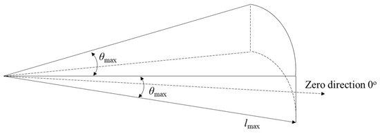
Figure 1.
The pursuit angle of the producer.
- Zero direction:
- Right-half side:
- Left-half side:
where θmax and lmax are the maximum pursuit angle and the maximum pursuit distance of the producer, respectively; θmax and lmax ∈ R1; θmax is calculated from where ; lmax is calculated from , where UBi and LBi are the upper and lower bounds of the ith dimension, respectively; r1 is a random variable of normal distribution between −1 and 1, and r1 ∈ R1; and r2 denotes a random variable uniformly distributed between 0 and 1, and r2 ∈ Rn−1.
If the above search strategy finds a fitness value better than the current one, it replaces the current position of the producer as the best individual position. Otherwise, it remains at the current position and the following strategy uses the following Equation (7) to update its pursuit angle:
where αmax is the maximum rotation angle of the producer, r2 is a random variable of uniform distribution between 0 and 1, and r2 ∈ Rn−1.
If the above strategy does not obtain a position with a better fitness value after a iterations, the pursuit angle is kept at the current angle .
In GSO, scroungers move closer to the producer. In the kth iteration, the search strategy of the ith scrounger is to update its position according to Equation (8) [46]:
where r3 is a random variable of uniform distribution between 0 and 1 and r3 ∈ Rn; is the Hadamard product.
From their current position, rangers perform a random search of the search space to conduct the exploitation as shown in Equation (9):
where li is the distance of the ith ranger according to a ∙ r1 ∙ 1max.
Figure 2 shows the flowchart of GSO algorithm. Initial members are generated during initialization and divided into producer, scroungers, and rangers based on fitness values. After a producer is created, its position is updated according to Equations (4)–(7). Scroungers are then updated according to Equation (8). Finally, rangers are updated according to Equation (9). If the stop condition is met, GSO stops and releases the solution.
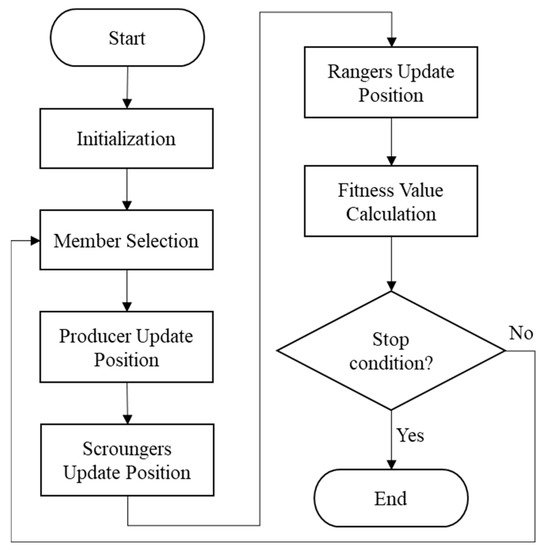
Figure 2.
Flowchart of GSO algorithm.
2.2. UD
The UD method first proposed by Wang and Fang [37] is a widely used experimental design method for investigating multiple factors and levels [41,42,43]. The UD, which is based on Quasi-Monte Carlo method, is implemented by low discrepancy sequence and integral. The UD method sacrifices orderliness and comparability in order to maximize the uniformity of dispersion needed to reduce limitations on the usage of factors and levels. In UD, a uniform layout is the experimental design arrangement tool. The Un(qs) represents the uniform layout, where U is the uniform layout, n is the number of experiments, q is the number of levels for factors, and s is the number of factors. The steps of establishing a uniform layout are as follows:
- Set the number of experiments nexp, and select a number h, where 1 is the greatest common divisor of n and h;
- Design the jth column in the uniform layout according to Equation (10):where uij is the element in the uniform layout, i.e., level, i and j means the ith row and jth column, respectively.
Table 1 is a U11(1110) uniform layout. Each column can place a factor in this table, and each row represents an experimental combination. The content of this table is the range of the level reference factor. For practical application and satisfaction of factors, columns can be selected partially. According to Wang and Fang [37], an even uniform layout can be obtained by an odd uniform layout by removing the last combination, e.g., U10(1010), shown as Table 2, can be obtained from U11(1110) by removing the 11th combination (row). However, to ensure the characteristic of uniform distribution in the uniform layout, every uniform layout has a usage table. Table 3 is the usage table for the U11 and U10 uniform layouts.

Table 1.
U11(1110) uniform layout.
Table 2.
U10(1010) uniform layout.
Table 3.
A usage table of the U11 and U10 uniform layouts.
2.3. Taguchi Method
The Taguchi method proposed by Taguchi [38] is a statistics-based experimental design method widely used to solve practical design issues, including parameter design, system design, and tolerance design [39]. Compared with the vast amount of experiments required for factorial experiments, the orthogonality of the Taguchi method substantially reduces experimental costs and simplifies data analysis. Taguchi method uses three static characteristics for evaluation indicators: the smaller-the-better characteristic, the nominal-the-best characteristic, and the larger-the-better characteristic. In this study, the Taguchi method is used to enhance the regional search capability of the GSO algorithm, and the smaller-the-better characteristic is used to analyze the factor response.
The Taguchi method uses an La(bc) orthogonal table to arrange experiments, where a is the number of experiments, b is the number of levels for each factor, and c is the maximum of factors. Table 4 is an L8(27) orthogonal table.
Table 4.
A usage table of the U11 uniform layout.
After the orthogonal table required for Taguchi method is established, the factor response table is established based on the SNR (signal-to-noise ratio, η) observed after the experiment [47] as shown in Equation (11):
where yit is the tth result of the ith experimental combination.
Table 5 is an example of the response table. The experimenter can determine whether a factor performs well and at which levels by comparing the response values at different levels.
Table 5.
A response table from the L8(27) orthogonal table.
Here, factor A is taken as an example to illustrate how to calculate the response value of each level.
ηA1 = (η1 + η2 + η3 + η4)/4
ηA2 = (η5 + η6 + η7 + η8)/4
Equations (12) and (13) can be used to evaluate the performance of each factor at different levels. First, η and the level of each factor should be collected and then averaged. The best factor level can then be obtained from the response table.
3. Proposed Method
This section briefly describes the methods applied in this paper. One method proposed elsewhere is using UD to search for the factor combination of the GSO algorithm. The robust-GSO (RGSO) method proposed here integrates the Taguchi method in the GSO algorithm to determine the best fitness value.
3.1. GSO Parameter Optimization by UD Method
The first step of the GSO algorithm is setting the percentage of ranger Xr, the initial angle φ0, the maximum pursuit angle of producer θmax, the maximum rotation angle of producer αmax, and the maximum pursuit distance of producer lmax. Since these five parameters have the most important roles in GSO performance, an efficient and accurate search for the best parameter combinations is critical. Conventional parameter optimization methods have major limitations, i.e., the trial-and-error experimental method is not systematic, and the full-factorial experimental method has a heavy calculation burden. Therefore, this paper selects a systematic and efficient method, the UD method, to search for the best parameter combination in terms of enhancing the adaptive diversity of the GSO algorithm. The recommended settings are as follows [8]:
- The percentage of ranger Xr is [0%, 100%];
- The initial angle φ0 is [π/8, π];
- The maximum pursuit angle of producer θmax is [π/2a2, 4π/a2];
- The maximum rotation angle of producer αmax is [θmax/8, θmax];
- The maximum pursuit distance of producer lmax is [lmax/8, 4lmax].
The range of each parameter is then used to establish the uniform layout required to search for the best parameter combination for the GSO algorithm. Figure 3 is a flowchart of optimal parameters for the GSO algorithm when the uniform layout is selected. The detailed explanation is as follows. First, the ranges of the parameters are divided into levels according to the recommended parameter settings. Based on the number of parameters and the usage table, U10(105) uniform layout can be obtained, as shown in Table 6. The levels were put into U10(105) uniform layout, and Table 7 can be obtained. Next, the parameter combination from Table 7 was taken into GSO orderly to set the parameters and GSO was performed to evaluate the benchmark functions until all experimental combinations of the U10(105) uniform layout are run at least once. Finally, the best combination is obtained. The best combination can make producers and rangers update to a better position and scrounges can follow them.
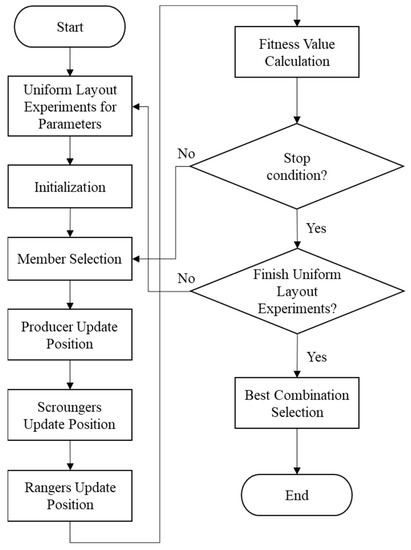
Figure 3.
Flowchart of parameter optimization procedure for the GSO algorithm when using the uniform layout.
Table 6.
A U10(105) uniform layout.
Table 7.
The U10(105) uniform layout for the GSO algorithm.
3.2. Robust-GSO Algorithm
The GSO algorithm uses the rangers to exploit the search results. The PS mechanism of the GSO algorithm then compares the fitness values of the producers and selects the producer that has the best fitness for exploring the solution.
Other individuals in the group are then moved close to the position of the individual with the best fitness value. If only a producer is selected for use in leading scroungers for positioning scroungers close to the best position, the local minimum would be easy to receive. Therefore, this paper proposes a multi-producer mechanism that improves the algorithmic capability of the GSO by integrating Taguchi method in the search for the best individual. Given the robust results obtained by integrating the Taguchi method, the proposed method is referred to as the robust-GSO algorithm (R-GSO).
The R-GSO first provides a flexible number of producers Xp. In each iteration the best and the second-best members (Xp1 and Xp2, respectively) are selected as the producers. To ensure diversity, one of the remaining producers is randomly selected to be the third producer, Xp3. The three producers, Xp1, Xp2, and Xp3, are then used to set the levels of variables when implementing Taguchi method. Thus, three crossover types are selected: Xp1 and Xp2 as the first and second levels, Xp1 and Xp3 as the first and second levels, and Xp2 and Xp3 as the first and second levels. Additionally, an Lm(2m−1) orthogonal table is selected. After the Taguchi method is performed, three new producers, Xnp1, Xnp2, and Xnp3, can be obtained, and then the one with the best performance among them is the optimal producer, Xop.
For example, each producer has five dimensions, i.e., Xp1 = (), Xp2 = (), and Xp3 = (). Table 8 shows an orthogonal table L8(27), and this table can satisfy the dimension, so it is used to determine the new producers. For illustration, Xp1 and Xp2 are adopted as the first and second levels, respectively. Because the dimension is five, the first five columns were selected for the crossover operation, and then each variable was put into the orthogonal table. Thus, Table 9 can be obtained. Table 9 shows the layout from Xp1 and Xp2 as the first and second levels, respectively. Based on the response table, a new producer, Xnp1, is obtainable. The Xnp2 and Xmp3 can also be obtained by applying this rule. The tunable parameters should be one more for matching this architecture. Thus, Table 10 shows that a U10(106) uniform layout must be selected to fit six parameters. Figure 4 is a flowchart of the R-GSO.
Table 8.
Example of L8(27) orthogonal table.
Table 9.
Example of crossover performed using L8(27) for Xp1 and Xp2 with 5 dimensions.
Table 10.
The U10(106) uniform layout with the tunable factors of R-GSO.
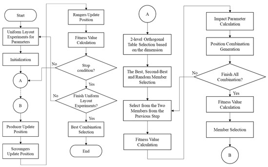
Figure 4.
Flowchart of R-GSO algorithm steps.
4. Experimental Results
In this study, the ten benchmark functions in Table 11 were used to evaluate the strengths and weaknesses of the proposed UD-GSO and R-GSO in comparison with the original GSO [8], where f1–f3 are unimodal functions, f4–f6 are multimodal functions, and f7–f10 are limited multimodal functions. For this evaluation, the iteration counts were set to 3000 for f1, f2, f3, f4, and f6; 5000 for f5 and f8; 150 for f7; and 200 for f9 and f10. The number of f1–f10 groups was set to 48. Each benchmark function was evaluated in 30 independent experiments, and the mean and standard deviation were used as benchmarks for performance evaluation. Mean values that approximated target (ftarget) values and small standard deviations were interpreted as indicators of good performance.
Table 11.
Benchmark functions used in this study.
The experimental results indicated that when parameters were set to preset values, the UD-GSO and R-GSO usually outperformed GSO. Table 12, Table 13 and Table 14 show the results from benchmark functions obtained for the GSO, UD-GSO, and R-GSO. Each combination was executed in 30 independent trials, and the combination with the best performance was selected. Because the characteristics of each function are inconsistent, the best combination of parameters needs to be selected based on the experimental layout from UD.
Table 12.
Results comparison among GSO [8], UD-GSO, and R-GSO in unimodal functions.
Table 13.
Results comparison among GSO [8], UD-GSO, and R-GSO in multimodal functions.
Table 14.
Results comparison among GSO [8], UD-GSO, and R-GSO in restricted multimodal functions.
4.1. Results of Unimodal Functions
In this study, the GSO, UD-GSO, and R-GSO were first performed using the unimodal functions. Table 12 shows the minimum, mean, and standard deviation (S.D.) of each function. In addition, Table 12 also shows the significant differences between UD-GSO vs. GSO and R-GSO vs. GSO, represented by the p-value from the t-distribution test. From Table 12, for the f1 function, the best parameter combination for UD-GSO was the ninth combination in Table 7, with a minimum of 1.9555 × 10⁻¹⁸, a mean of 1.2741 × 10⁻¹⁵, and an S.D. of 4.0520 × 10⁻¹³. The best parameter combination for R-GSO was the fourth one in Table 10, with a minimum of 4.6597 × 10⁻¹⁴, a mean of 7.1195 × 10⁻¹¹, and an S.D. of 1.5407 × 10⁻¹¹. The p-values from the t-distribution test are 3.6553 × 10⁻⁴ and 3.6557 × 10⁻⁴ for UD-GSO vs. GSO and R-GSO vs. GSO, respectively. For the f2, the best parameter combination for UD-GSO was the ninth combination in Table 7, with a minimum of 0.1372, a mean of 0.4594, and an S.D. of 0.1898. The best parameter combination for R-GSO was the eighth one in Table 10, with a minimum of 0.1845, a mean of 0.3524, and an S.D. of 0.0730. The p-values from the t-distribution test are 1.1263 × 10⁻⁴ and 0.0289 for UD-GSO vs. GSO and R-GSO vs. GSO, respectively. For the f3, the best parameter combination for UD-GSO was the ninth combination in Table 7, with a minimum of 1.1797, a mean of 44.3206, and an S.D. of 30.9214. The best parameter combination for R-GSO was the fourth one in Table 10, with a minimum of 6.9507, a mean of 19.1942, and an S.D. of 30.6621. The p-values from the t-distribution test are 0.0482 and 2.0700 × 10⁻⁴ for UD-GSO vs. GSO and R-GSO vs. GSO, respectively. From the above results, it can be seen that there is a significant difference between UD-GSO and R-GSO in terms of the p-value of t-distribution; in terms of mean, UD-GSO and R-GSO are smaller than GSO, but in f1, UD-GSO has a better performance than R-GSO. Although the minimum in f1, f2, and f3 obtained by UD-GSO is smaller than R-GSO, R-GSO has a more robust performance than UD-GSO in f2 and f3 based on S.D. Additionally, because each function’s characteristics are inconsistent, the best combinations of parameters must be selected based on the uniform layout.
4.2. Results of Multimodal Functions
Next, this paper evaluated the performance of the GSO, UD-GSO, and R-GSO using multimodal functions. Table 13 also shows each function’s minimum, mean, and S.D. and the p-value from the t-distribution test between UD-GSO vs. GSO and R-GSO vs. GSO. From Table 13, for the f4 function, the best parameter combination for UD-GSO was the seventh combination in Table 7, with a minimum of −12,569.4866, a mean of −12,569.4858, and an S.D. of 0.0013. The best parameter combination for R-GSO was the eighth in Table 10, with a minimum of −12,569.4866, a mean of −12,569.4866, and an S.D. of 0.0002. The p-values from the t-distribution test are 5.6422 × 10⁻⁷ and 5.6421 × 10⁻⁷ for UD-GSO vs. GSO and R-GSO vs. GSO, respectively. For the f5, the best parameter combination for UD-GSO was the ninth combination in Table 7, with a minimum of 8.3805 × 10⁻¹⁶, a mean of 1.5842, and an S.D. of 1.3657. The best parameter combination for R-GSO was the eighth one in Table 10, with a minimum of 2.2971 × 10⁻¹⁶, a mean of 1.1219, and an S.D. of 1.1252. The p-values from the t-distribution test are 6.1909 × 10⁻⁹ and 3.4610 × 10⁻⁹ for UD-GSO vs. GSO and R-GSO vs. GSO, respectively. For the f6, the best parameter combination for UD-GSO was the ninth combination in Table 7, with a minimum of 1.1490 × 10⁻¹⁹, a mean of 1.1963 × 10⁻¹⁴, and an S.D. of 6.4158 × 10⁻¹⁴. The best parameter combination for R-GSO was the fourth one in Table 10, with a minimum of 1.1218 × 10⁻¹⁶, a mean of 1.3433 × 10⁻¹³, and an S.D. of 3.0473 × 10⁻¹³. The p-values from the t-distribution test are both 0.0026 for UD-GSO vs. GSO and R-GSO vs. GSO. The results show a significant difference between UD-GSO and R-GSO in terms of the p-value of t-distribution; in terms of performance in mean and standard deviation, the performance of UD-GSO and R-GSO is better than GSO. Compared with UD-GSO, R-GSO has a better mean and S.D. in f4 and f5, but in f6 the mean and S.D. obtained by UD-GSO are better than R-GSO. Because each function’s characteristics are inconsistent, the best parameter combinations were selected by the uniform layout.
4.3. Results of Restricted Unimodal Functions
Last, this paper takes the restricted unimodal functions for the performance evaluation of the GSO, UD-GSO, and R-GSO. Table 14 also shows each function’s minimum, mean, and S.D. and the p-value from the t-distribution test between UD-GSO vs. GSO and R-GSO vs. GSO. From Table 14, for the f7 function, the best parameter combination for UD-GSO was the eighth combination in Table 7 (minimum of 0.9980; mean of 0.9980; and S.D. of 0.0013) and for R-GSO was the ninth one in Table 10 (minimum of 0.9980; mean of 0.9980; and S.D. of 0.0002). The p-values from the t-distribution test are NaN for UD-GSO vs. GSO and R-GSO vs. GSO because the evaluation values are close. For the f8, the best parameter combination for UD-GSO was the fifth combination in Table 7 (minimum of 3.0749 × 10⁻⁴; mean of 3.4302 × 10⁻⁴; and S.D. of 1.9042 × 10⁻⁴) and for R-GSO was the eighth one in Table 10 (minimum of 3.0749 × 10⁻⁴; mean of 3.6912 × 10⁻⁴; and S.D. of 2.3457 × 10⁻⁴). The p-values from the t-distribution test are 0.0164 and 0.0389 for UD-GSO vs. GSO and R-GSO vs. GSO, respectively. For the f9, the best parameter combination for UD-GSO was the eighth combination in Table 7 (minimum of 3; mean of 3; and S.D. of 1.4060 × 10⁻¹⁴) and for R-GSO was the tenth one in Table 10 (minimum of 3; mean of 3; and S.D. of 1.0981 × 10⁻¹⁴). The p-values from the t-distribution test are NaN for UD-GSO vs. GSO and R-GSO vs. GSO because the evaluation values are close. For the f10, the best parameter combination for UD-GSO was the third combination in Table 7 (minimum of −10.1519; mean of −7.7473; and S.D. of 2.7845) and for R-GSO was the seventh one in Table 10 (minimum of −10.1530; mean of −8.1125; and S.D., 2.6089). The p-values from the t-distribution test are 0.1346 and 0.0428 for UD-GSO vs. GSO and R-GSO vs. GSO, respectively. The results show a significant difference between UD-GSO and R-GSO in terms of the p-value of t-distribution in f8 and f10; in terms of mean performance, both UD-GSO and R-GSO are smaller than GSO in f8 and f10, and UD-GSO and R-GSO have the same mean to GSO in f7 and f9; in addition, in terms of standard deviation, R-GSO performs better than UD-GSO in f7 to f10. The best combinations of parameters were selected by the uniform layout because each function’s characteristics are inconsistent.
5. Conclusions
This paper describes how the experimental design method was used to optimize the performance of the GSO algorithm. Comparisons of benchmark functions confirmed that the proposed UD-GSO and R-GSO indeed improved performance in comparison with the original GSO proposed by He et al. [8]. Specifically, the proposed GSO algorithm improves solution quality and robustness in comparison with the original GSO. Experimental performance comparisons also confirmed that compared with the original GSO the proposed UD-GSO and R-GSO provide superior calculation results in terms of robustness and convergence based on experimental results, as shown in Table 12, Table 13 and Table 14. Notably, however, UD-GSO outperforms R-GSO in terms of computing time. Therefore, future studies can investigate whether further optimization of the parameter settings of the algorithm improve performance. If a fine resolution is a need, it is necessary to increase the number of experiments to explore the hyperparameters. Due to the characteristic of the Taguchi method, the number of experiments using an orthogonal array increases as the dimension increases in geometric progression, so it is not recommended to use R-GSO in a higher dimension. Notably, however, the relative importance of computational cost is expected to decrease as technological advances yield further increases in computing power. The desired target value achieves the effect of improving the overall performance. Therefore, the key performance metric will continue to be the effectiveness of the algorithm in terms of its capability to find the target value required for improvement in overall performance.
Author Contributions
Conceptualization, methodology, project administration, F.-I.C. and J.-H.C.; validation, W.-H.H., F.-I.C. and J.-H.C.; software, formal analysis, P.-Y.Y. and K.-Y.Y.; writing—original draft preparation, P.-Y.Y., K.-Y.Y. and F.-I.C.; supervision, W.-H.H. and J.-H.C.; funding acquisition, P.-Y.Y., W.-H.H., F.-I.C. and J.-H.C. All authors have read and agreed to the published version of the manuscript.
Funding
This research was funded by National Science and Technology Council, Taiwan (R.O.C.), grant number MOST-111-2221-E-153-006, MOST 111-2221-E-992-072-MY2 and MOST 110-2221-E-035-092-MY3. The APC was funded by National Science and Technology Council, Taiwan (R.O.C.), grant number MOST 110-2221-E-035-092-MY3.
Institutional Review Board Statement
Not applicable.
Informed Consent Statement
Not applicable.
Data Availability Statement
Not applicable.
Conflicts of Interest
The authors declare no conflict of interest.
References
- LaValle, S.M.; Branicky, M.S.; Lindemann, S.R. On the relationship between classical grid search and probabilistic roadmaps. Int. J. Robot. Res. 2004, 23, 673–692. [Google Scholar] [CrossRef]
- Ruder, S. An overview of gradient descent optimization algorithms. arXiv 2016, arXiv:1609.04747. [Google Scholar]
- Alatas, B.; Bingöl, H. Comparative Assessment of Light-based Intelligent Search and Optimization Algorithms. Light Eng. 2020, 28, 51–59. [Google Scholar] [CrossRef]
- Whitley, D. A genetic algorithm tutorial. Stat. Comput. 1994, 4, 65–85. [Google Scholar] [CrossRef]
- Mori, K.; Tsukiyama, M.; Fukuda, T. Immune algorithm with searching diversity and its application to resource allocation problem. IEEJ Trans. Electron. Inf. Syst. 1993, 113, 872–878. [Google Scholar]
- Dorigo, M.; Birattari, M.; Stutzle, T. Ant colony optimization. IEEE Comput. Intell. Mag. 2006, 1, 28–39. [Google Scholar] [CrossRef]
- Kennedy, J.; Eberhart, R. Particle swarm optimization. In Proceedings of the ICNN’95—International Conference on Neural Networks, Perth, Australia, 27 November–1 December 1995. [Google Scholar]
- He, S.; Wu, Q.H.; Saunders, J.R. Group search optimizer: An optimization algorithm inspired by animal searching behavior. IEEE Trans. Evol. Comput. 2009, 13, 973–990. [Google Scholar] [CrossRef]
- Mirjalili, S.; Lewis, A. The whale optimization algorithm. Adv. Eng. Softw. 2016, 95, 51–67. [Google Scholar] [CrossRef]
- Chou, F.-I.; Huang, T.-H.; Yang, P.-Y.; Lin, C.-H.; Lin, T.-C.; Ho, W.-H.; Chou, J.-H. Controllability of Fractional-Order Particle Swarm Optimizer and Its Application in the Classification of Heart Disease. Appl. Sci. 2021, 11, 11517. [Google Scholar] [CrossRef]
- Zhao, T.-F.; Chen, W.-N.; Liew, A.W.-C.; Gu, T.; Wu, X.-K.; Zhang, J. A Binary Particle Swarm Optimizer with Priority Planning and Hierarchical Learning for Networked Epidemic Control. IEEE Trans. Syst. Man Cybern. Syst. 2021, 51, 5090–5104. [Google Scholar] [CrossRef]
- Kumar, P.; Shilpi, S.; Kanungo, A.; Gupta, V.; Gupta, N.K. A Novel Ultra Wideband Antenna Design and Parameter Tuning Using Hybrid Optimization Strategy. Wirel. Pers. Commun. 2022, 122, 1129–1152. [Google Scholar] [CrossRef]
- Boursianis, A.D.; Papadopoulou, M.S.; Salucci, M.; Polo, A.; Sarigiannidis, P.; Psannis, K.; Mirjalili, S.; Koulouridis, S.; Goudos, S.K. Emerging Swarm Intelligence Algorithms and Their Applications in Antenna Design: The GWO, WOA, and SSA Optimizers. Appl. Sci. 2021, 11, 8330. [Google Scholar] [CrossRef]
- Pujari, H.K.; Rudramoorthy, M. Grey wolf optimisation algorithm for solving distribution network reconfiguration considering distributed generators simultaneously. Int. J. Sustain. Energy 2022, 41, 2121–2149. [Google Scholar] [CrossRef]
- Shekarappa, G.S.; Mahapatra, S.; Raj, S. Voltage Constrained Reactive Power Planning Problem for Reactive Loading Variation Using Hybrid Harris Hawk Particle Swarm Optimizer. Electr. Power Compon. Syst. 2021, 49, 421–435. [Google Scholar] [CrossRef]
- Ren, M.; Zhang, Q.; Yang, Y.; Wang, G.; Xu, W.; Zhao, L. Research and Application of Reservoir Flood Control Optimal Operation Based on Improved Genetic Algorithm. Water 2022, 14, 1272. [Google Scholar] [CrossRef]
- Lord, S.A.; Shahdany, S.H.; Roozbahani, A. Minimization of Operational and Seepage Losses in Agricultural Water Distribution Systems Using the Ant Colony Optimization. Water Resour. Manag. 2021, 35, 827–846. [Google Scholar] [CrossRef]
- Bisewski, D. Application of the Genetic Algorithm in the Estimation Process of Models Parameters of Semiconductor Devices. Prz. Elektrotechniczny 2022, 98, 103–106. [Google Scholar]
- Kaur, G.; Gill, S.S.; Rattan, M. Whale Optimization Algorithm Approach for Performance Optimization of Novel Xmas Tree-Shaped FinFET. Silicon 2022, 14, 3371–3382. [Google Scholar] [CrossRef]
- Mavrovouniotis, M.; Li, C.; Yang, S. A survey of swarm intelligence for dynamic optimization: Algorithms and applications. Swarm Evol. Comput. 2017, 33, 1–17. [Google Scholar] [CrossRef]
- Billaut, J.C.; Moukrim, A.; Sanlaville, E. Flexibility and Robustness in Scheduling; Wiley Online Library: New York, NY, USA, 2008. [Google Scholar]
- Chen, C.H.; Chou, F.I.; Chou, J.H. Multiobjective evolutionary scheduling and rescheduling of integrated aircraft routing and crew pairing problems. IEEE Access 2020, 8, 35018–35030. [Google Scholar] [CrossRef]
- Yang, P.Y.; Chou, F.I.; Tsai, J.T.; Chou, J.H. Adaptive-uniform-experimental-design-based fractional-order particle swarm optimizer with non-linear time-varying evolution. Appl. Sci. 2019, 9, 5537. [Google Scholar] [CrossRef]
- Tsai, J.T.; Chou, P.Y.; Chou, J.H. Color filter polishing optimization using ANFIS with sliding-level particle swarm optimizer. IEEE Trans. Syst. Man Cybern. Syst. 2017, 50, 1193–1207. [Google Scholar] [CrossRef]
- Abualigah, L.; Diabat, A. Chaotic binary group search optimizer for feature selection. Expert Syst. Appl. 2022, 192, 116368. [Google Scholar] [CrossRef]
- Daryani, N.; Hagh, M.T.; Teimourzadeh, S. Adaptive group search optimization algorithm for multi-objective optimal power flow problem. Appl. Soft Comput. 2016, 38, 1012–1024. [Google Scholar] [CrossRef]
- Chang, P.Y.; Chou, F.I.; Yang, P.Y.; Chen, S.-H. Hybrid multi-object optimization method for tapping center machines. Intell. Autom. Soft Comput. 2023, 36, 23–38. [Google Scholar] [CrossRef]
- Yang, W.; Guo, J.; Vartosh, A. Optimal economic-emission planning of multi-energy systems integrated electric vehicles with modified group search optimization. Appl. Energy 2022, 311, 118634. [Google Scholar] [CrossRef]
- Abualigah, L. Group search optimizer: A nature-inspired meta-heuristic optimization algorithm with its results, variants, and applications. Neural Comput. Appl. 2020, 33, 2949–2972. [Google Scholar] [CrossRef]
- Beauchamp, G.; Giraldeau, L.A. Group foraging revisited: Information sharing or producer-scrounger game? Am. Nat. 1996, 148, 738–743. [Google Scholar] [CrossRef]
- Basu, M. Quasi-oppositional group search optimization for hydrothermal power system. Int. J. Electr. Power Energy Syst. 2016, 81, 324–335. [Google Scholar] [CrossRef]
- Zhang, X.; Chan, K.W.; Wang, H.; Zhou, B.; Wang, G.; Qiu, J. Multiple group search optimization based on decomposition for multi-objective dispatch with electric vehicle and wind power uncertainties. Appl. Energy 2020, 262, 114507. [Google Scholar] [CrossRef]
- Teimourzadeh, H.; Jabari, F.; Mohammadi-Ivatloo, B. An augmented group search optimization algorithm for optimal cooling-load dispatch in multi-chiller plants. Comput. Electr. Eng. 2020, 85, 106434. [Google Scholar] [CrossRef]
- Teimourzadeh, H.; Mohammadi-Ivatloo, B. A three-dimensional group search optimization approach for simultaneous planning of distributed generation units and distribution network reconfiguration. Appl. Soft Comput. 2020, 88, 106012. [Google Scholar] [CrossRef]
- Xi, S.; Xu, Y.; Li, M.; Ji, T.; Wu, Q. Two-stage diagnosis framework for heating pipeline system using improved group search optimizer. Energy Build. 2023, 280, 112715. [Google Scholar] [CrossRef]
- Starch, D. A demonstration of the trial and error method of learning. Psychol. Bull. 1910, 7, 20. [Google Scholar] [CrossRef]
- Fang, K.T.; Lin, D.K.; Winker, P.; Zhang, Y. Uniform design: Theory and application. Technometrics 2000, 42, 237–248. [Google Scholar] [CrossRef]
- Taguchi, G.; Chowdhury, S.; Taguchi, S. Robust Engineering; McGraw-Hill: New York, NY, USA, 2000. [Google Scholar]
- Roy, R.K. A Primer on the Taguchi Method; Society of Manufacturing Engineers: Southfield, MI, USA, 2010. [Google Scholar]
- Bell, W.J. Searching Behaviour: The Behavioural Ecology of Finding Resources; Springer Science and Business Media: Heidelberg/Berlin, Germany, 2012. [Google Scholar]
- Wang, Y.; Fang, K.T. A note on uniform distribution and experimental design. Chin. Sci. Bull. 1981, 26, 485–489. [Google Scholar]
- Fang, K.T. Uniform Design and Uniform Layout; Science Press: Beijing, China, 1994. [Google Scholar]
- Tsao, H.; Lee, L. Uniform layout implement on MATLAB. Stat. Decis. 2008, 2008, 144–146. [Google Scholar]
- Mustard, D. Numerical Integration over the n-Dimensional Spherical Shell. Math. Comput. 1964, 18, 578–589. [Google Scholar]
- Barnard, C.J.; Sibly, R.M. Producers and scroungers: A general model and its application to captive flocks of house sparrows. Anim. Behav. 1981, 29, 543–550. [Google Scholar] [CrossRef]
- Giraldeau, L.A.; Lefebvre, L. Exchangeable producer and scrounger roles in a captive flock of feral pigeons: A case for the skill pool effect. Anim. Behav. 1986, 34, 797–803. [Google Scholar] [CrossRef]
- Tsai, J.T.; Liu, T.K.; Chou, J.H. Hybrid Taguchi-genetic algorithm for global numerical optimization. IEEE Trans. Evol. Comput. 2004, 8, 365–377. [Google Scholar] [CrossRef]
Disclaimer/Publisher’s Note: The statements, opinions and data contained in all publications are solely those of the individual author(s) and contributor(s) and not of MDPI and/or the editor(s). MDPI and/or the editor(s) disclaim responsibility for any injury to people or property resulting from any ideas, methods, instructions or products referred to in the content. |
© 2023 by the authors. Licensee MDPI, Basel, Switzerland. This article is an open access article distributed under the terms and conditions of the Creative Commons Attribution (CC BY) license (https://creativecommons.org/licenses/by/4.0/).