Abstract
Groundwater is the most abundant freshwater resource. Agriculture, industrialization, and domestic water supplies rely on it. The depletion of groundwater leads to drought. Topographic elevation, aquifer properties, and geomorphology influence groundwater quality. As the groundwater level data (GWL) are time series in nature, it is challenging to determine appropriate metrics and to evaluate groundwater levels accurately with less information loss. An effort has been made to forecast groundwater levels in India by developing a deep ensemble learning approach using a double-edge bi-directed long-short-term-memory (DEBi-LSTM) model approximated with a randomized low-ranked approximation algorithm (RLRA) and the variance inflation factor (VIF) to reduce information loss and to preserve data consistency. With minimal computation time, the model outperformed existing state-of-the-art models with accuracy. To ensure sustainable groundwater development, the proposed work is discussed in terms of its managerial implications. By applying the model, we can identify safe, critical, and semi-critical groundwater levels in Indian states so that strategic plans can be developed.
1. Introduction
Water is a renewable energy that protects the ecosystem. At the same time, fresh water is a limited and costly resource. Water conservation encompasses the strategies, policies, and activities to manage fresh water as a sustainable resource to balance current and future human demand. A UNICEF report indicates that half of the world’s population will live in areas where water is scarce by 2025 [1]. Multiple stressful events across a wide range are inextricably linked to water scarcity. Water stress results in a global risk for water demand and water unavailability. When the natural elements are unable to meet the essential demand for water, it has a serious effect on the functionality of the ecosystem. The extensive impact of water scarcity has been shown in several large cities in India such as Punjab, Rajasthan, Haryana, Uttar Pradesh, Karnataka, Tamil Nadu, and Andhra Pradesh [2]. In any socio-economic civilization development, groundwater is the most desirable resource; and of necessary water demand in rural and urban areas is covered by groundwater storage [3]. Acute water demands affect industry, agriculture, health, and the economy, so there is concern about the sustainability of groundwater resources. Groundwater depletion includes the reduction of water in streams, the deterioration of water quality, and land subsidence. In 2003, NASA’s Gravity Recovery and Climate Experiment (GRACE) satellite gathered data on GWL changes in south India, and it concluded that GWL increased before 2009, but since then, it has decreased at a rate of cm/month, as studied by [4]. From 2003 to 2009 and after 2009, the changes in GWL have been recorded as two segments, as noted in [4]. Nevertheless, GWL simulations represent an integrated response to geological, topographic, and hydrological factors, making them challenging.
Over the past two decades, artificial intelligence (AI) models have been widely employed to address the drawbacks of conventional methods for GWL stimulation. Due to the dynamic and heterogeneous nature of GWL, it is difficult to conduct simulations with high accuracy and comprehensiveness. The following Figure 1 depicts the state-wise GWL rise and fall in India from 2010 to 2020, where 0 to 100 represents the rise of the waterbed level and 0 to represents the fall of the waterbed level. A rise is considered an increase in the availability of the water level under the land surface, and a fall is considered the decline of the water level from the saturated zone. This study abbreviates the Indian states according to the Indian template, as mentioned in [5]
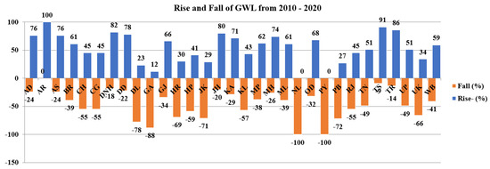
Figure 1.
State–wise groundwater level fluctuation (2010–2020).
Numerous studies have been undertaken regarding groundwater, such as groundwater quality investigations, surface water level estimation, observations on organic components in the drinking water, groundwater contamination, and many more using a sundry simulation approach. These approaches can be conceptual, experimental, or numerical models. Out of these groundwater level predictions arises an interesting need of time due to severe climate changes. It has been observed that groundwater level predictions were carried out using smart techniques such as machine learning, deep learning techniques, and ensemble learning. Some of the related works are depicted below.
1.1. Review on Groundwater Level Prediction Using Machine Learning Technique
Knoll et al. [6] proposed a prediction model for identifying the nitrate level of aquatic factors by statistical and machine learning (ML) techniques and found that random forest (RF) produces better performance with a maximum R-value. Majumdar et al. [7] studied the impact of aquifer exhaustion by monitoring groundwater extraction using a multi-variate regression method and RF with a good value. Adiat et al. [8] predicted GWL using geoelectric parameters and explored the process by an artificial neural network (ANN) using RMSE and the regression coefficient. Hussein et al. [9] compared the various ML techniques and found that support-vector regression (SVR) produces good accuracy for measuring the availability of groundwater to mitigate the sustainability and scarcity problem. Banadkooki et al. [10] hybridized a neural network with the Whale algorithm for hyperparameter optimization using an adaptive neuro-fuzzy interface system (ANFIS).
Even though machine learning techniques show better prediction accuracy, they have the limitation of stimulating a reduced amount of data. As the data increases, there is a chance for less prediction accuracy. Additionally, some machine learning techniques lack in identifying the best attributes to support the prediction process, where feature selection takes a major role. Furthermore, comparatively, the computation time is high as there is an increase in the training process. Thus, to overcome these issues, researchers have directed their attention towards deep learning techniques in groundwater level prediction.
1.2. Review on Groundwater Level Prediction Using a Deep Learning Technique
In recent studies, deep learning (DL) techniques have shown an extensive prospect in the prediction field by refining the predictive parameters that have the ability to assess enormous amounts of data. Huang et al. [11] compared the performance of ML with DL techniques and found that long short-term memory (LSTM) produced better predictions for groundwater recharge. Chen et al. [12] studied the existence of potential groundwater levels contrary to the high demand for renewable groundwater levels and presented better validation accuracy. Kochhar et al. [13] partitioned the available dataset into pre-monsoon, post-monsoon, and combined annual datasets for measuring the groundwater level with a seasonal auto-regressive integrated moving average (SARIMA) model with LSTM. Sun et al. [14] proposed a data-driven model for groundwater level prediction with practical significance using ARIMA and LSTM. Oyedele et al. [15] developed a DL framework that is tuned by a genetic algorithm to produce a generalized prediction over daily pricing. Jimenez-Mesa et al. [16] designed a non-parametric framework to estimate the statistical significance for classification by combining an auto-encoder with a support-vector machine (SVM).
Even though deep learning has the ability to process huge data, its prediction depends on various influential parameters, which may affect the prediction accuracy of using a particular classifier. Additionally, it suffers from the limitation of high computation cost with data inconsistency, leading us to take steps for the data acquisition process. Furthermore, overfitting is one of the significant issues to be taken care of with a better algorithm selection process with an efficient hyperparameter tuning process. Thus, combining more than one classifier may improve the prediction process and pave the way for the ensemble learning mechanism.
1.3. Review on Groundwater Level Prediction Using Ensemble Learning
Due to the growing demand for the more accurate prediction of groundwater levels, the ensemble model has presented a quality evaluation which is essential for the precise identification of influential parameters. A machine learning-based ensemble model was analyzed by Mosavi et al. Ref. [17] proposed an ensemble-based model using boosted regression tree (BRT) and random forest (RF) to estimate the groundwater hardness. Yin et al. [18] proposed a machine learning-based ensemble model with ANN, SVM, and response surface regression to perform the weak-strong learner’s decision-making process. Jiang et al. [19] proposed a multi-model perturbation-based algorithm to perturb the feature space using bootstrap sampling to provide a better solution. Mosavi et al. [20] proposed a design with GAMBoost and AdaBoost for a boosting method, and their bagging method was designed with a classification and regression tree (CART) and RF mode. Lee et al. [21] proposed a DL-based ensemble model using long short-term memory (LSTM), gated recurrent units (GRU), and a multi-layered perceptron (MLP) for predicting the erythrocyte sediment rate. Li et al. [22] proposed a DL-based ensemble model designed using a recurrent neural network (RNN) and a fully connected neural network for analyzing future stock movements. Ngo et al. [23] developed an ML-based ensemble learning process using ANN, SVR, and M-5 rules to predict energy consumption in buildings.
From the previous related work, the following gaps are identified, which motivates the identification of the problem statement to propose the research model. The identified gaps are as follows:
- Machine learning methods struggle to handle enormous amounts of data in groundwater level prediction for huge geographical regions.
- Deep learning techniques have high computation time, and it is difficult to identify the better algorithm with hyperparameters upon feature selection in groundwater level prediction.
- Identifying the primary attributes for groundwater prediction is tedious, as every attribute has its own advantages and disadvantages that affect the generalization mechanism.
- Data pre-processing techniques used in the previous research led to information loss and, in turn, reduced the prediction accuracy.
One of the challenging tasks in prediction depends on understanding the data pattern. Even though smart techniques help us with learning adaptability, the selection of an algorithm with the model’s potentiality depends on the evaluation of performance metrics with less information loss. As the groundwater level is characterized by various factors such as geological, topological, and hydrological properties, it is mandatory to pre-process the data to maintain data consistency. These considerations and limitations motivate us to identify the significant attributes using the variance inflation factor (VIF) using the multi-collinearity test. The reduced dataset is further approximated using randomized low-rank approximation (RLRA) to reduce the computation cost of the training process. Thus, the proposed model uses RLRA and VIF for data consistency, whereas a deep ensemble model (DEM) using double-edge bi-directed LSTM (DEBi-LSTM) provides improved prediction accuracy. The objectives of the paper are as follows:
- To obtain attributes using multi-collinearity by applying the variance inflation factor (VIF) value;
- To obtain the data approximation using the randomized low-rank approximation (RLRA) technique over the attribute selection;
- To combine random forest as a base learner using a stacking mechanism and double-edge bi-directional LSTM as a meta-classifier to obtain the deep ensemble Model (DEM);
- To find better classification accuracy, the DEM was applied to both approximated and non-approximated reduced datasets;
- To reduce the overfitting using the proposed DEM mechanism;
- To check for minimal or no information loss during data approximation to maintain data authenticity;
- To calculate the time taken to train and to test the data iteratively to assess the computation cost.
The article is articulated as follows: the introduction discusses the need for groundwater and the existing groundwater level in the states of India, followed by the related research activities carried out in Section 1. Background fundamentals are discussed in Section 2. The proposed research methodology on groundwater level prediction is emphasized in Section 3 with feature selection and approximation processes, whereas Section 4 explains the experimental analysis according to the deep ensemble model. Section 5 explains the results and discussion. Section 6 describes the comparative analysis with existing research methods. Section 7 illustrates the managerial implication of the proposed groundwater prediction process. Section 8 follows with conclusions and future work.
2. Background Fundamentals
One of the important tasks in the prediction process includes data collection and data pre-processing. After data collection, analyzing and organizing the data into valuable insights improves the decision-making process. Pre-processing involves identifying the relationship between the attribute values of the collected data, and identifying the significant attributes helps in reducing the computation time and cost. To find the correlation between the dependent and independent variables and remove the predictors that are less likely to represent the prediction process using the multi-collinearity test is a more challenging task that can be achieved using VIF. Thus, we utilized VIF in our model.
2.1. Variance Inflation Factor (VIF)
Predictive models deal with various influential parameters that improve the efficiency of the decision-making process. The variance inflation factor (VIF) determines the correlation between the independent variables. The independent variables are represented as , . The VIF threshold, , is indicated as the threshold value for attribute selection. Algorithm 1 shows the process of attribute selection using VIF. Let us explain the process of VIF using a sample information system, represented in Table 1 and in Example 1. The variance inflation factor for the ith attribute is shown in Equation (1):
| Algorithm 1 Feature selection using variance inflation factors |
Parameters:
Input: Input matrix is . Output: Reduced dataset is . Procedure to calculate the VIF value
|

Table 1.
Information System.
Example 1.
A sample information system is given in Table 1. where the attributes are chlorine, Cl, represented as , magnesium, Mg, represented as , manganese, Mn, represented as , iron, Fe, represented as , calcium, Ca, represented as , Zinc, Zn, represented as , and copper, Cu, represented as .
On considering the attribute (Chlorine), the VIF is calculated using Equation (1) as follows:
Thus, a summary is given in Table 2.
Table 2.
VIF number with the corresponding attribute values.
From Table 2, it can be seen that the attributes , and have a VIF value less than the considered threshold of 5. The information system is now reduced with attributes. Again, the reduced information system checked with the VIF values and found there is no change in the attributes to be reduced. Thus, the reduced information system is given in Table 3.
Table 3.
Reduced information system.
2.2. Randomized Low-Rank Approximations
Data approximation plays a major role in reducing complex calculations into less complicated ones. Most data modeling works better for certain and less complex datasets. An appropriate approximation model helps in performing the decision-making process better with complex datasets. If the knowledge base has a huge number of attributes with various ranges of data, the computation complexity can be reduced by finding the rank of the space. Thus, we utilized the randomized low-rank approximation (RLRA) technique in the research model [24,25]. The method of approximating a matrix by a relatively lower rank matrix is known as a low-rank approximation. The goal is to achieve a further compact representation of the original data set with limited loss of information.
In this section, let us discuss the basics of the RLRA technique.
- (i)
- Singular Value Decomposition (SVD)
Any real matrix of arbitrary size can be factored or decomposed into a product of orthonormal matrices and diagonal matrices, such as Equation (2):
where U and V both have orthonormal columns, and whose columns contain, respectively, the left and right singular vectors. The diagonal matrix contains singular values corresponding to the singular vectors. We denote the ith singular value as and order them and their corresponding singular vectors into U and V such that diag and for all i. This is represented as Equation (3),
which is a decomposition of Y into a sum of rank-l matrices. Here, and ; note that the eigenvectors of are , and the eigenvectors of are . Each one has the eigenvalues .
- (ii)
- Orthogonal Projections
Assume we have an orthonormal basis for a linear subspace that has been stacked into a matrix: . Then, is a projection matrix that, when applied to a matrix , projects it orthogonally onto the subspace spanned by Q, which we denote as in Equation (4):
- (iii)
- Norms
Two matrix norms are commonly used to keep things simple and easy to compare—the Frobenius norm, Equation (5), and the norm, Equation (6).
The Frobenius norm is as follows:
The operator norm is as follows:
where, for vectors is the standard (Euclidean) norm .
- (iv)
- Optimal Randomized Low-Rank Decomposition
The motivation for using the Frobenius and norm for the RLRA method was supported by the classical result from [26], which states that the best rank-k approximation to is achieved by truncating the singular values (setting for ). There always exists a set of columns and multiplicative factor of those to produce the optimal solution [27].
Table 3 attribute values are approximated by Algorithm 2 and represented in Table 4. By approximation using the RLRA algorithm, minimal information loss is achieved, which ensures that the authenticity of the data remains unchanged. Figure 2 visualizes the heatmap structure of the reduced information system and the RLRA-information system to represent the color variation of numerical data, while preserving the data’s authenticity. Figure 3 represents the graphical similarity behavior of the RLRA algorithm to the reduced information system and the approximated information system.
| Algorithm 2 Approximation using RLRA. |
Parameters:
Input: Input matrix . Output: Reduced matrix . Procedure:
|
Table 4.
Approximate information system.
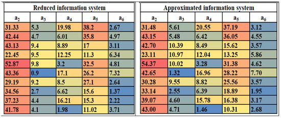
Figure 2.
Heatmap of reduced information system and approximated information system.
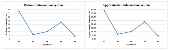
Figure 3.
Similarity check against reduced information system and approximated information system.
2.3. Ensemble Learning
In general, ensemble learning is based on the baseline classifiers for dependent or independent methods. In dependent methods, the result of one classifier has an impact on the next classifier’s formation. Some of the examples are boosting algorithms [28,29,30]. On the other hand, the independent methods build each classifier separately from the subset of the data and combine its results [7,8,9,31]. Various ensemble techniques have been proposed for the successful improvement of predictive accuracy [17,18,20]. The final predictive model requires a proper combination of several learners. The combination of these classifiers is divided into averaging and meta-learning. Simple ensemble techniques come under averaging methods, whereas advanced ensemble techniques include stacking, blending, bagging, and boosting methods. As our proposed model aims to improve predictive accuracy, the stacking ensemble approach will be discussed.
2.3.1. Stacking Ensemble Learning
Stacking is a powerful ensemble learning mechanism. The base learners are stacked in a parallel manner by combining with the meta learners to obtain better prediction accuracy. The general architecture of the stacking mechanism is given in Figure 4. It consists of two or more base learner models and meta-models combined to form a predictive model. The data are divided into folds and partitioned into training and testing data. The base learners are triggered with the predictions as first-level predictions on the training data. The meta-model helps to combine the predictions of the first level, and the prediction pattern is trained on other models to obtain the prediction accuracy.
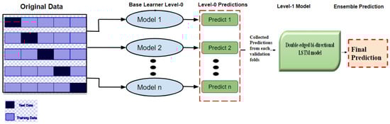
Figure 4.
Generalized architecture of ensemble learning process.
3. Proposed Research Methodology on Groundwater Level Prediction
3.1. Study Area Investigation and Data Pre-Processing
The paper aims to investigate the groundwater level in India. Groundwater level data were collected from all the districts of India from 2000 to 2021. As per the census of India, 593 districts were counted in the years 2001 to 2010, whereas 640 districts were counted from 2011 to 2020. The census of India reported 773 districts from the year 2021. Thus, the data collected are from 2000 to 2021 and have the objects of 13,103 records. For a better understanding of the data pattern, India was divided into four divisions, such as East and Northeast India, encompassing the states Arunachal Pradesh, Assam, Meghalaya, Nagaland, Manipur, Mizoram, Tripura, Sikkim, West Bengal, Jharkhand, Bihar; Northwest India includes the states Uttar Pradesh, Uttarakhand, Haryana, Chandigarh, Delhi, Punjab, Himachal Pradesh, Jammu, Kashmir, and Rajasthan. Central India includes the Nicobar Islands, Madhya Pradesh, Gujarat, Dadra, Nagar Haveli, Daman and Diu, Goa, Maharashtra, and Chhattisgarh, whereas South India includes Andhra Pradesh, Telangana, Tamil Nadu, Puducherry, Karnataka, Kerala, Lakshadweep, Andaman, and the Nicobar Islands, as represented in Figure 5. The groundwater sampling was carried out from representative borewells in various districts of every state of India through web resources [32]. With consultation with the domain expert, the variables that have a significant impact on GWL are listed in Table 5. As per the expert advice, the data were collected on three main factors, such as geological, topological, and hydrological properties, as given in Figure 6. The collected data underwent pre-processing to check their consistency. Out of 13,103 objects, 387 records had missing data, and 716 pieces of data had conflicting information, leading to the data removal process. Thus, 12,000 records were considered for processing, whereas 1103 records were removed. It is essential to identify significant attributes that contribute better to the knowledge discovery process of groundwater levels. As the collected data are independent of each other, finding the inter-relations or inter-associations between the attributes can be recognized using the multi-collinearity test with the help of variance inflation factors (VIF). Therefore, the following section deals with identifying significant attributes using the multi-collinearity test.
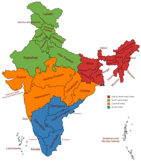
Figure 5.
Four divisions of India.
Table 5.
Notation table.
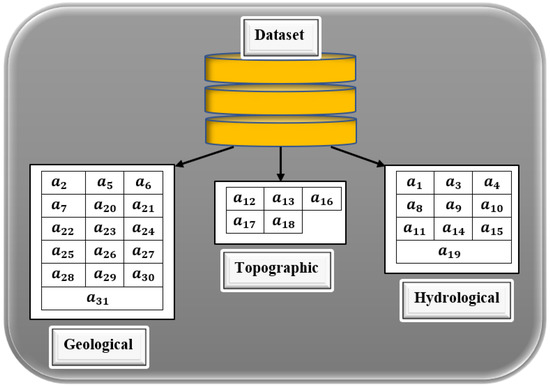
Figure 6.
Properties of input variables.
3.2. Feature Selection Using Multi Collinearity Test
This section aims to identify the selection of significant attributes using a multi-collinearity test. For each attribute, variance inflation factors (VIF) identify the multi-collinearity number using Equation (1), where the unadjusted determination coefficient for the ith independent attribute over the other attributes is determined by . The VIF threshold value () was assumed on a better understanding of the data pattern. For the collected data with a dimension of 12,000 × 32, the VIF is calculated on each attribute and discards the attributes that fail to have an association in the prediction process. The process of VIF calculation is given in Algorithm 1. The calculated VIF values for all 32 attributes are depicted in Table 6. Figure 7 clearly illustrates the attribute reduction process, and better features are selected. The reduced sample dataset with 18 attribute values is presented in Figure 8.
Table 6.
VIF calculation for 32-attributes.
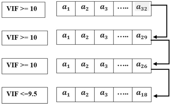
Figure 7.
Attribute reduction.
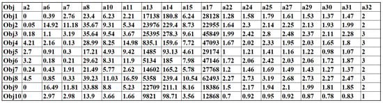
Figure 8.
Sample dataset.
3.3. Attribute Approximation Using Randomized Low-Rank Approximation Method
After the attribute selection through the VIF number of the corresponding column, the rank of the reduced dataset was checked using the rank function of MATLAB. The rank function identified that the reduced dataset was of rank 18. The basics of RLRA are explained in Section 2.2 with Algorithm 2. The sample dataset is depicted in Figure 8.
The real rank of the dataset was 18, but it was approximated by the RLRA technique, which obtained 3 as the reduced rank. Figure 9 shows the approximated dataset of the sample dataset.
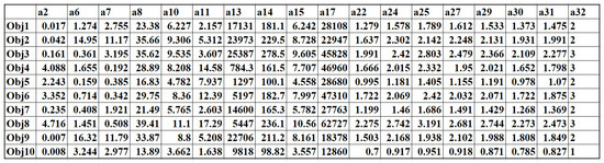
Figure 9.
Approximated dataset using RLRA.
To depict the data authenticity, a heat map and similarity representation were created for both the original sample dataset and approximated data, as shown in Figure 10 and Figure 11. It can be seen that the data distribution on the knowledge base is almost the same for both datasets. Thus, data authenticity is maintained. The approximated and non-approximated dataset is further applied to the deep ensemble learning process.
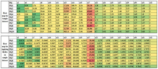
Figure 10.
Heat map for sample and approximated dataset.
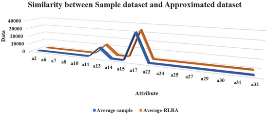
Figure 11.
Similarity between sample dataset and approximated dataset.
3.4. Proposed Deep Ensemble Model
The main idea of the proposed ensemble method is to combine the assorted base classifiers into different layers. The first layer (Level 0) trains the group of deep base learners on a different partition of the training dataset to form a so-called team. In the next layer, Level 1, a group of meta-classifiers is trained on the prediction of the team of Level 0. In the final layer, the predictions of the previous group of classifiers are combined with the meta-classifier to produce the results. Figure 12 shows the stacking mechanism of the proposed model, as discussed in Section 2.3.1.
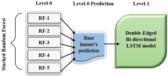
Figure 12.
Stacking mechanism of proposed model.
3.4.1. Proposed Deep Ensemble Architecture
The proposed deep ensemble model encompasses random forest (RF) as the base learner and double-edged bi-directional LSTM (DEBi-LSTM) as the meta-classifier [33,34]. The reduced dataset from the randomized low-rank approximation is partitioned into training data of and testing data of and fed into the deep ensemble model. The overall learning architecture of the proposed ensemble is depicted in Figure 13. The architecture makes use of two levels of classifiers . Each training fold is applied into the random forest (RF) as a base learner . The output of the base learner in each fold is combined with the DEBi-LSTM using a meta classifier and produces the output. The proposed architecture is similar to a multi-layer perceptron, with Level 0 representing the input layer, Level 1 representing the hidden layer, and the output layer. The meta-classifier (DEBi-LSTM) uses the ‘Relu’ activation function by taking the input from the base learner and producing the output in the final layer. Let us discuss the design of the proposed double-edged bi-directional LSTM before the training process.
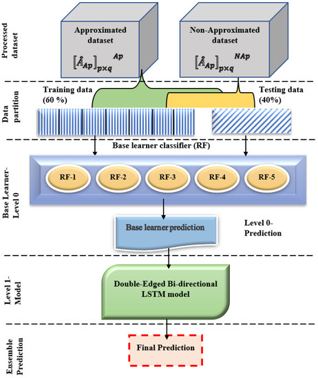
Figure 13.
Architecture of proposed ensemble model.
3.4.2. Double-Edged Bi-Directional LSTM
The first hidden layer of the bi-directional connection is configured with 128 LSTM memory units through the ‘Relu’ activation function, whereas the return sequence must be true to allow passage into the output from the prior layer to the next subsequent layer. The first layer is narrowed using the dropout layer as . The second hidden layer is stacked with 64 LSTM memory units by the ‘Relu’ activation function, and the dropout layer is configured as . Hereafter, two dense layers and 3, respectively) are separated by a dropout layer equal to . A fully connected layer followed by this above architecture for obtaining the prediction output is called a dense layer. The design of the proposed DEBi-LSTM is represented in Figure 14.
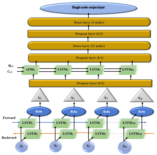
Figure 14.
Design of proposed DEBi-LSTM.
3.4.3. Proposed Training Process
The training phase took the input of both the approximated (AP) data from RLRA and the non-approximated reduced (NAP) data to be fed into Level 1 of the base learner. Given the dataset , the procedure selected random n samples of equal size for each dataset. Each sample was partitioned into training and testing data. = . The Level 0 classifier was generated using RF to each with a learning rate. Hence, the first fold with the learning rate was called a team. A collection of teams was , , represented as , where to 5, team. Each produced the prediction as of a sample n to be fed as input to the next level, Level 1. Once the Level 1 fed with the previous layer prediction was finished with the meta-classifier, double-edge bi-directional LSTM (DEBi-LSTM) trained the as . Subsequently, the generated the data based on the meta-classifier to produce the final output, . The overall training process is illustrated in Algorithm 3.
| Algorithm 3 Ensemble model for groundwater level prediction |
Parameter:
|
4. Experimental Analysis According to Deep Ensemble Model
This section deals with the experimental analysis of the base classifiers that were implemented using online Google Colab. To implement the meta-classifier, we used the scikit-learn python library, which includes various machine learning algorithms. To evaluate the proposed deep ensemble approach to the predictions, the experiment was conducted on the two reduced datasets, the approximated dataset and the non-approximated dataset, of the groundwater level. To train the baseline classifiers in the teams, it is necessary to divide the training data using data partitioning methods. Our proposed model adopted the k-fold partitioning method, which randomly divides the training set into equal-size partitions. As the training data are of a total of 7200 objects, there were 12 partitions, each having 600 training objects. A team of base learners (random forest) was applied in each split in Level 0. The predictions from the base learner were applied to the DEBi-LSTM model of Level 1 to obtain the final classification accuracy of both the approximated and non-approximated datasets. The empirical analysis of the proposed ensemble model with the hyperparameters are provided in Table 7 and Table 8.
Table 7.
Choice and best choice of hyper-parameters.
Table 8.
Classification accuracy of approximated and non-approximated data on DEM.
Performance Analysis Using Evaluation Metrics
The performance analysis of the proposed model was carried out using the following evaluation metrics: accuracy, (Equation (7)), precision, (Equation (8)), recall, (Equation (9)), score, and (Equation (10)). These points are related to the evaluation metrics: True correct classification (TCc), True non-correct classification (TNCc), False correct classification (FCc), False non-correct classification (FNCc).
5. Result and Discussion
The performance of the proposed researched model of DEM was verified by tuning the hyper-parameters, such as the batch size, number of epochs, number of memory units, number of dropouts, learning rate, and the optimizer, represented in Table 7. By comparing the training performance for the various choice options, the best hyper-parameters can be identified. Table 8 illustrates the classification performance for the approximated and non-approximated datasets. Each dataset was analysed independently with the related three batch sizes. At a batch size of 32, the approximated dataset had the highest classification accuracy of 91.26%. In the case of the non-approximated dataset, the classification accuracy was 89.26%. Moreover, the 12 splits provided the best classification accuracy. Having this information at hand will help support the argument that the approximated dataset is superior to the non-approximated dataset.
The training performance with the various batch sizes and iteration processes is shown in Table 9. Here, with a batch size of 32, the approximated dataset (AP) requires the lowest number of iterations to achieve the best training performance with respect to , , , and compared with the non-approximated dataset. Additionally, it is observed that the proposed DEM produces better performance with a batch size of 32, as represented in Figure 15.
Table 9.
Training iteration for approximated and non-approximated datasets.
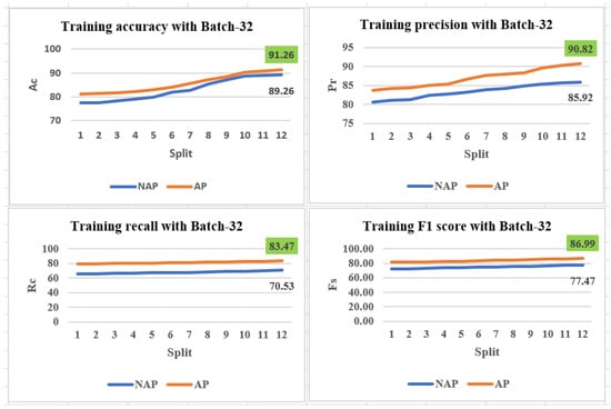
Figure 15.
Training performance with a batch size of 32.
Based on the classification accuracy obtained using the approximated and non-approximated data, along with the evaluation of the performance analysis, we had the confidence to select the approximated dataset with a batch size of 32 to obtain the prediction accuracy. The obtained prediction accuracy is listed in Table 10.
Table 10.
Prediction accuracy for approximated and non-approximated dataset.
From Table 10, batch-32 produced 96.1% accuracy for the approximated dataset, where as 93.76% accuracy for the non-approximated dataset. The 12 splits provide the best classification accuracy. Thus, there is an increase in prediction accuracy of 2.34% for the simulated approximated dataset. For the approximated dataset the evaluation metrics such as , , and show their values as , , and respectively, which is shown in Figure 16.
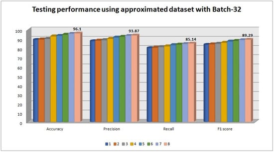
Figure 16.
Testing performance with batch size 32.
6. Comparative Analysis with Existing Research Methods
A comparative analysis has been carried out with the proposed model against the model designed by [35] using LSTM, also compared to a model proposed by [20] using Bagging-ensemble, and compared by ensemble model proposed by [18]. Table 11 has given the justification regarding the choice of the proposed model and demonstrated the prediction analysis with the approximated dataset where the proposed DEM model achieved the highest , , and comparing with the existing deep learning, and an ensemble model. Here, the ensemble model [18] is designed with the conventional machine learning techniques so while the data size is huge and the model is working over the varieties of data characteristics, prediction performance is reduced. Among LSTM [35], and Bagging-ensemble [20], the prediction performance shows better in the case of the bagging-ensemble process because the prediction process is suppressed with the conventional LSTM for the overfitting problem.
Table 11.
Comparative analysis with deep learning, benchmarked ensemble models and proposed model.
Figure 17 demonstrates a comparative analysis using the accuracy with a split of 8. It is shown that the proposed DEM has achieved the comparatively highest accuracy, with a value of , using the approximated dataset with a batch size 32 among the existing benchmakred deep learning ensemble models.
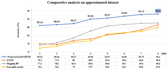
Figure 17.
Comparative analysis with deep learning [35], benchmarked ensemble models [18,20] and proposed model with approximated dataset.
7. Managerial Implications of the Proposed Groundwater Prediction Process
Depletion of groundwater levels is a major concern for India, as of the world’s total population depends on water. Moreover, irrigation purposes, domestic demand, and the industrial use of water impose over-exploitation on the country’s groundwater level [36]. This major water crisis might project severe water stress in the near future. Realizing the water crisis, the study has highlighted some of the concerning factors that are considered regarding their parametric value for implementation.
- Natural water rechargeability is average.
- Its utility for irrigation, industrial, and domestic purpose is high.
- Population growth is huge.
Erratic water rechargeability and increasing water demand cause endangered water stress for the states of Northwest India, such as Gujarat, Madhya Pradesh, and Maharashtra, in Central India, and in Telangana, Tamil Nadu, and Puducherry in South India. The following Table 12 shows the past 8-year rainfall pattern for the above-mentioned states [37]. These states are recorded as critical to semi-critical zones for highly stressed GWL. By the proposed DEM process, this study has categorized the statewide GWL of India, represented in Figure 18. GWL are strongly correlated with annual rainfall. GWL is gradually reduced due to the excessive need for power generation, population demand, irrigation, and industrialization. The present study thus points out the states of India according to their predicted GWL. As the sources of natural water resources is becoming minimal due to various climatic changes, the implication of that water usage must be reduced by a measured amount. Thus, the seasonal uncertainty of rainfall could not affect the GWL as well as it would help to fulfill the essential demands for living purposes. This effort will help prevent the issue of the decline in the water table in India.
Table 12.
Rainfall pattern of the past 8 years (2015–2022).
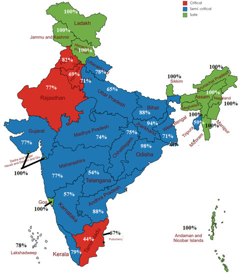
Figure 18.
DEM predicts state-wise GWL of India.
8. Conclusions and Future Work
The reliable prediction and accurate estimation of the depletion of groundwater level to refine the efficacy of water usage leads to a better, more sustainable water resource management system. The prediction capability has been esteemed over the substantial attribute. The attributes considered for the study depend on three contingency factors to represent the closeness of the attributes with groundwater sustainability as geological, topographic, and hydrological properties. The weather system in tropical regions such as India is controlled by convection and radiation and involves a non-linear association with rainfall, which is the main source of groundwater. Thus, the salient features are identified using the variance inflation factor from the collected data. As significant features always contribute better predictions for consistent data, they have been obtained using the randomized low-rank approximation technique for the reduced dataset. The consistent data are partitioned into training and testing sets, which are employed in the proposed deep ensemble model for the classification and prediction process. The approximated and non-approximated datasets are employed in the proposed model to check the classification accuracy, as discussed in Section 4. Section 5 discusses the analysis of the experimental results and exhibits an improved tuning of hyperparameters, with the meta-classifier showing that the approximated data have a 2% increase in classification accuracy compared to the non-approximated data. Similarly, the prediction accuracy was increased by 2.34% for the approximated data compared to the non-approximated data. Additionally, the proposed deep ensemble model has proved to have better classification and prediction capacities when it is compared against the benchmarked existing techniques as provided in Section 6. Since groundwater levels are strongly dependent on rainfall, and due to various climatic changes, annual rainfall may diminish or overflow, creating fluctuations in the GWL. Thus, the accuracies obtained by the proposed model are validated by the GWL prediction through 2022, and we found that the model prediction and the status updated by the government’s categorization are almost the same. Thus, the same is shown in Figure 18, where groundwater levels are categorized as critical, semi-critical, or safe. The proposed model can be improved using some optimization techniques to tune the hyperparameters to reduce the computation time and improve the accuracy.
Author Contributions
All authors equally contributed to the manuscript. Conception and design, material preparation, data collection, and analysis were performed by T.M. and A.A. All authors have read and agreed to the published version of the manuscript.
Funding
This research was funded by the School of Information Technology and Engineering, Vellore Institute of Technology, Vellore 632014, Tamil Nadu, India.
Institutional Review Board Statement
Not applicable.
Informed Consent Statement
Not applicable.
Data Availability Statement
Not applicable.
Conflicts of Interest
The the authors declare no conflict of interest.
Abbreviations
The following abbreviations are used in this manuscript:
| UNICEF | United Nations Children’s Fund |
| NASA | National Aeronautics and Space Administration |
| GRACE | Gravity Recovery and Climate Experiment |
| GWL | Groundwater level |
| AI | Artificial intelligence |
| RF | Random forest |
| ML | Machine learning |
| ANN | Artificial neural network |
| RMSE | Root-mean-square error |
| SVR | Support-vector regression |
| ANFIS | Adaptive neuro-fuzzy inference system |
| DL | Deep learning |
| LSTM | Long short-term memory |
| SARIMA | Seasonal autoregressive integrated moving average |
| SVM | Support-vector machine |
| BRT | Boosted regression trees |
| CART | Classification and regression tree |
| GRU | Gated recurrent units |
| MLP | Multi-layer perceptron |
| RNN | Recurrent neural network |
| RLRA | Randomized low-rank approximation |
| VIF | Variance inflation factor |
| DEM | Deep ensemble model |
| DEBi-LSTM | Double-edge bi-directional LSTM |
References
- Water Scarcity. Available online: https://www.unicef.org/wash/water-scarcity (accessed on 20 May 2022).
- Space Applications Centre, ISRO. Desertification and Land Degradation Atlas of Selected Districts of India (Based on IRS LISS III data of 2011–13 and 2003–05); Space Applications Centre (ISRO): Ahmedabad, India, 2016; pp. 1–219. [Google Scholar]
- Chindarkar, N.; Grafton, R.Q. India’s depleting groundwater: When science meets policy. Asia Pac. Policy Stud. 2019, 6, 108–124. [Google Scholar] [CrossRef]
- Rodell, M.; Houser, P.R.; Jambor, U.; Gottschalck, J.; Mitchell, K.; Meng, C.-J.; Arsenault, K.; Cosgrove, B.; Radakovich, J.; Bosilovich, M.; et al. The Global Land Data Assimilation System. Bull. Am. Meteorol. Soc. 2004, 85, 381–394. [Google Scholar] [CrossRef]
- India State Map, List of States in India. Available online: https://www.whereig.com/india/states/ (accessed on 20 May 2022).
- Knoll, L.; Breuer, L.; Bach, M. Large scale prediction of groundwater nitrate concentrations from spatial data using machine learning. Sci. Total Environ. 2019, 668, 1317–1327. [Google Scholar] [CrossRef] [PubMed]
- Majumdar, S.; Smith, R.; Butler, J.J., Jr.; Lakshmi, V. Groundwater withdrawal prediction using integrated multitemporal remote sensing data sets and machine learning. Water Resour. Res. 2020, 56, e2020WR028059. [Google Scholar] [CrossRef]
- Adiat, K.A.N.; Ajayi, O.F.; Akinlalu, A.A.; Tijani, I.B. Prediction of groundwater level in basement complex terrain using artificial neural network: A case of Ijebu-Jesa, southwestern Nigeria. Appl. Water Sci. 2020, 10, 1–14. [Google Scholar] [CrossRef]
- Hussein, E.A.; Thron, C.; Ghaziasgar, M.; Bagula, A.; Vaccari, M. Groundwater prediction using machine-learning tools. Algorithms 2020, 13, 300. [Google Scholar] [CrossRef]
- Banadkooki, F.B.; Ehteram, M.; Ahmed, A.N.; Teo, F.Y.; Fia, C.M.; Afan, H.A.; Sapitang, M.; Shafie, A.E. Enhancement of Groundwater-Level Prediction Using an Integrated Machine Learning Model Optimized by Whale Algorithm. Nat. Resour. Res. 2020, 29, 3233–3252. [Google Scholar] [CrossRef]
- Huang, X.; Gao, L.; Crosbie, R.S.; Zhang, N.; Fu, G.; Doble, R. Groundwater recharge prediction using linear regression, multi-layer perception network, and deep learning. Water 2019, 11, 1879. [Google Scholar] [CrossRef]
- Chen, Y.; Chen, W.; Chandra Pal, S.; Saha, A.; Chowdhuri, I.; Adeli, B.; Janizadeh, S.; Dineva, A.A.; Wang, X.; Mosavi, A. Evaluation efficiency of hybrid deep learning algorithms with neural network decision tree and boosting methods for predicting groundwater potential. Geocarto Int. 2021, 37, 1–21. [Google Scholar] [CrossRef]
- Kochhar, A.; Singh, H.; Sahoo, S.; Litoria, P.K.; Pateriya, B. Prediction and forecast of pre-monsoon and post-monsoon groundwater level: Using deep learning and statistical modelling. Model. Earth Syst. Environ. 2022, 8, 2317–2329. [Google Scholar] [CrossRef]
- Sun, J.; Hu, L.; Li, D.; Sun, K.; Yang, Z. Data-driven models for accurate groundwater level prediction and their practical significance in groundwater management. J. Hydrol. 2022, 608, 127630. [Google Scholar] [CrossRef]
- Oyedele, A.A.; Ajayi, A.O.; Oyedelec, L.O.; Bello, S.A.; Jimoh, K.O. Performance evaluation of deep learning and boosted trees for cryptocurrency closing price prediction. Expert Syst. Appl. 2022, 213, 119233. [Google Scholar] [CrossRef]
- Jiménez-Mesa, C.; Ramírez, J.; Suckling, J.; Vöglein, J.; Levin, J.; Górriz, J.M.; DIAN, D.I.A.N. Deep Learning in current Neuroimaging: A multivariate approach with power and type I error control but arguable generalization ability. arXiv 2021, arXiv:2103.16685. [Google Scholar] [CrossRef]
- Mosavi, A.; Hosseini, F.S.; Choubin, B.; Abdolshahnejad, M.; Gharechaee, H.; Lahijanzadeh, A.; Dineva, A.A. Sustainability prediction of groundwater hardness using ensemble machine learning models. Water 2008, 12, 2770. [Google Scholar] [CrossRef]
- Yin, J.; Medellín-Azuara, J.; Escriva-Bou, A.; Liu, Z. Bayesian machine learning ensemble approach to quantify model uncertainty in predicting groundwater storage change. Sci. Total Environ. 2021, 769, 144715. [Google Scholar] [CrossRef]
- Jiang, F.; Yu, X.; Du, J.; Gong, D.; Zhang, Y.; Peng, Y. Ensemble learning based on approximate reducts and bootstrap sampling. Inf. Sci. 2021, 547, 797–813. [Google Scholar] [CrossRef]
- Mosavi, A.; Hosseini, F.S.; Choubin, B.; Goodarzi, M.; Dineva, A.A.; Rafiei Sardooi, E. Ensemble boosting and bagging based machine learning models for groundwater potential prediction. Water Resour. Manag. 2021, 35, 23–37. [Google Scholar] [CrossRef]
- Lee, J.; Hong, H.; Song, J.M.; Yeom, E. Neural network ensemble model for prediction of erythrocyte sedimentation rate (ESR) using partial least squares regression. Sci. Rep. 2022, 12, 1–13. [Google Scholar] [CrossRef]
- Li, Y.; Pan, Y. A novel ensemble deep learning model for stock prediction based on stock prices and news. Int. J. Data Sci. Anal. 2022, 13, 139–149. [Google Scholar] [CrossRef]
- Ngo, N.T.; Pham, A.D.; Truong, T.T.H.; Truong, N.S.; Huynh, N.T.; Pham, T.M. An ensemble machine learning model for enhancing the prediction accuracy of energy consumption in buildings. Arab. J. Sci. Eng. 2022, 47, 4105–4117. [Google Scholar] [CrossRef]
- Kumar, N.K.; Schneider, J. Literature survey on low rank approximation of matrices. Linear Multilinear Algebra 2017, 65, 2212–2244. [Google Scholar] [CrossRef]
- Sapp, B.J. Randomized Algorithms for Low-Rank Matrix Decomposition; Computer and Information Science, University of Pennsylvania: Philadelphia, PA, USA, 2011; pp. 1–43. [Google Scholar]
- Eckart, C.; Young, G. The approximation of one matrix by another of lower rank. Psychometrika 1936, 1, 211–218. [Google Scholar] [CrossRef]
- Halko, N.; Martinsson, P.G.; Tropp, J.A. Finding structure with randomness: Probabilistic algorithms for constructing approximate matrix decompositions. SIAM Rev. 2011, 53, 217–288. [Google Scholar] [CrossRef]
- Mohammed, A.; Kora, R. An effective ensemble deep learning framework for text classification. J. King Saud-Univ. Inf. Sci. 2022, 34, 8825–8837. [Google Scholar] [CrossRef]
- Chen, W.; Lei, X.; Chakrabortty, R.; Pal, S.C.; Sahana, M.; Janizadeh, S. Evaluation of different boosting ensemble machine learning models and novel deep learning and boosting framework for head-cut gully erosion susceptibility. J. Environ. Manag. 2021, 284, 112015. [Google Scholar] [CrossRef] [PubMed]
- Konstantinov, A.V.; Utkin, L.V. Interpretable machine learning with an ensemble of gradient boosting machines. Knowl.-Based Syst. 2021, 222, 106993. [Google Scholar] [CrossRef]
- Ma, M.; Liu, C.; Wei, R.; Liang, B.; Dai, J. Predicting machine’s performance record using the stacked long short-term memory (LSTM) neural networks. J. Appl. Clin. Med. Phys. 2022, 23, e13558. [Google Scholar] [CrossRef]
- Ground Water Data Access. Available online: http://cgwb.gov.in/GW-data-access.html (accessed on 20 May 2022).
- Hochreiter, S.; Schmidhuber, J. Long short-term memory. Neural Comput. 1997, 9, 1735–1780. [Google Scholar] [CrossRef]
- Hochreiter, S. Untersuchungen zu Dynamischen Neuronalen Netzen. Diploma Thesis, TU Munich, Munich, Germany, 1991. [Google Scholar]
- Park, C.; Chung, I.M. Evaluating the groundwater prediction using LSTM model. J. Korea Water Resour. Assoc. 2020, 53, 273–283. [Google Scholar] [CrossRef]
- India Groundwater: A Valuable but Diminishing Resource. Available online: https://www.worldbank.org/en/news/feature/2012/03/06/india-groundwater-critical-diminishing (accessed on 20 May 2022).
- India Water Resources Information System. Available online: https://indiawris.gov.in/wris/#/groundWater (accessed on 20 May 2022).
Disclaimer/Publisher’s Note: The statements, opinions and data contained in all publications are solely those of the individual author(s) and contributor(s) and not of MDPI and/or the editor(s). MDPI and/or the editor(s) disclaim responsibility for any injury to people or property resulting from any ideas, methods, instructions or products referred to in the content. |
© 2023 by the authors. Licensee MDPI, Basel, Switzerland. This article is an open access article distributed under the terms and conditions of the Creative Commons Attribution (CC BY) license (https://creativecommons.org/licenses/by/4.0/).