BTDNet: A Multi-Modal Approach for Brain Tumor Radiogenomic Classification

Abstract

Brain tumors pose significant health challenges worldwide, with glioblastoma being one of the most aggressive forms. The accurate determination of the O6-methylguanine-DNA methyltransferase (MGMT) promoter methylation status is crucial for personalized treatment strategies. However, traditional methods are labor-intensive and time-consuming. This paper proposes a novel multi-modal approach, BTDNet, that leverages multi-parametric MRI scans, including FLAIR, T1w, T1wCE, and T2 3D volumes, to predict the MGMT promoter methylation status. BTDNet’s main contribution involves addressing two main challenges: the variable volume lengths (i.e., each volume consists of a different number of slices) and the volume-level annotations (i.e., the whole 3D volume is annotated and not the independent slices that it consists of). BTDNet consists of four components: (i) data augmentation (which performs geometric transformations, convex combinations of data pairs, and test-time data augmentation); (ii) 3D analysis (which performs global analysis through a CNN-RNN); (iii) routing (which contains a mask layer that handles variable input feature lengths); and (iv) modality fusion (which effectively enhances data representation, reduces ambiguities, and mitigates data scarcity). The proposed method outperformed state-of-the-art methods in the RSNA-ASNR-MICCAI BraTS 2021 Challenge by at least 3.3% in terms of the F1 score, offering a promising avenue for enhancing brain tumor diagnosis and treatment.

1. Introduction

Brain tumors are a complex and heterogeneous group of neoplasms that pose a significant health challenge worldwide. Despite considerable progress in our understanding of their molecular and genetic underpinnings, the diagnosis, prognosis, and treatment of brain tumors remain formidable tasks [1,2]. In recent years, the integration of radiological imaging data with genomic information has emerged as a promising avenue in the field of neuro-oncology. This intersection of radiology and genomics, often referred to as “radiogenomics”, has the potential to revolutionize the approach to brain tumor characterization and classification [3].

The inherent complexity and diversity of brain tumors, coupled with the limitations of traditional histopathological methods, have spurred the search for non-invasive, complementary approaches to improve the accuracy of diagnosis and prognosis. Radiogenomic analysis leverages advanced imaging techniques, such as magnetic resonance imaging (MRI), computed tomography (CT), and positron emission tomography (PET), to extract a wealth of quantitative and qualitative imaging features [4,5]. These features are then correlated with the genetic and molecular characteristics of brain tumors, offering insights into their underlying biology and clinical behavior.

Glioblastoma, the most aggressive and prevalent primary brain tumor in adults, remains a therapeutic challenge despite advances in neuro-oncology [6]. The genetic and epigenetic heterogeneity within glioblastoma underscores the urgent need for precise biomarkers to guide personalized treatment strategies. Among these, the methylation status of the O6-methylguanine-DNA methyltransferase (MGMT) promoter has emerged as a critical determinant of the response to temozolomide, the standard chemotherapy for glioblastoma. The predictive power of the MGMT promoter methylation status in glioblastoma treatment outcomes underscores the significance of accurate and timely determination [6,7]. Traditionally, the determination of the MGMT promoter methylation status has relied on labor-intensive and time-consuming laboratory techniques, such as methylation-specific polymerase chain reaction (MSP) and pyrosequencing.

The emergence of AI-driven methods promises to revolutionize this process by analyzing high-dimensional genomic and epigenomic data. In this work, we utilize multi-parametric MRI (mpMRI) scans to address the prediction of the MGMT promoter methylation status at the pre-operative baseline MRI scans. The mpMRI scans consist of different types of 3D volumes (which constitute different modalities for the developed methodology): (a) fluid-attenuated inversion recovery (FLAIR); (b) native (i.e., T1-weighted pre-contrast or, in other words, T1w); (c) T1-weighted post-contrast (T1wCE); and (d) T2-weighted (T2) 3D volumes.

The challenges in using such 3D volumes of data for predicting the MGMT promoter methylation status are twofold: (i) the annotations are at the volume level rather than at the slice level, i.e., there exists one annotation for the whole volume; and (ii) the volumes have variable lengths, i.e., the volumes are 3D signals consisting of series of slices, i.e., 2D images, and each volume consists of a different number of images. The main contribution of this work is that our proposed method effectively addresses and overcomes these two challenges.

Traditional approaches handle 3D signals using 3D CNN architectures that generate one prediction per signal [8,9]; however, such architectures are very complex with a large number of parameters and require pre-training with other large 3D databases. In the healthcare domain and the medical imaging world, large 3D databases, annotated for the purpose of interest, are not easy to find, and in most cases, they are not publicly available due to privacy issues, regulatory frameworks, and policies. Other traditional approaches posit a hypothesis and assign the volume-level label to each slice of the volume, then employ CNN-RNN networks to train with the annotated slices. However, the fact that the whole volume has one label does not mean that each slice in the volume exhibits the MGMT promoter methylation status; it could be the case that only some slices display the MGMT promoter methylation status.

In cases where the volumes have variable lengths, traditional approaches use ad hoc strategies. They select a fixed volume length and either remove slices when a larger length is encountered (thus losing information that could be important for the final decision) or duplicate slices when the volume contains a smaller number of slices (this duplication negatively affects the final decision, as the model becomes biased toward the repeating data) [10,11,12]. Moreover, this ad hoc way of selecting the fixed volume length needs empirical tuning for each different database.

In this paper, we propose BrainTumorDetectionNetwork (BTDNet), a multi-modal approach for predicting the MGMT promoter methylation status. We develop a multi-modal approach, as leveraging data from multiple modalities helps the method (i) have a richer data representation since different modalities provide complementary information; (ii) reduce redundancy and ambiguity in data interpretation; and (iii) mitigate data scarcity.

BTDNet takes as input an mpMRI scan, i.e., a FLAIR 3D volume, a T1w 3D volume, a T1wCE 3D volume, and a T2 3D volume. BTDNet consists of four components: (i) data augmentation; (ii) 3D analysis; (iii) routing; and (iv) modality fusion. At first, while training, each input volume is passed through the data augmentation component, which initially applies geometric transformations to the input volume and then performs a novel augmentation technique on it. It should be noted that, during inference, we apply test-time data augmentation [13] to the input volume. The transformed input volume is then processed by the 3D analysis and routing components.

The 3D analysis component consists of a CNN network acting as a feature extractor and is applied to each slice of the volume. The features are then fed to an RNN that captures temporal information within the slices of the same volume. The RNN’s features are then passed to the routing component, consisting of a mask layer, which dynamically selects specific RNN outputs, followed by a dense layer (i.e., fully connected layer equipped with batch normalization [14] and a GELU [15]), whose output features are then fed to the modality fusion component. The mask layer is utilized for handling variable input feature lengths (due to variable slices per volume) when training the network.

The 3D analysis and routing components are identical and share the same weights for each of the four input 3D volumes (modalities). This means that there exist four identical 3D analysis and routing components. The modality fusion component is fed with the outputs of the routing component of all four modalities; these outputs are first concatenated and then fed to a dense layer that maps them to the same feature space. Then, the output layer follows and performs the final classification. Our method is trained using an extension of the focal loss [16] for multi-class classification.

The rest of this paper is organized as follows. Section 2 provides a comprehensive review of related works that address the problem of predicting the MGMT promoter methylation status. Section 3 presents the proposed method, along with its novelties. In addition, the dataset and pre-processing techniques utilized are described, along with the performance metrics used to evaluate our approach and the implementation details regarding our approach. Section 4 presents the rich experimental study in which we compare our method’s performance to that of the state-of-the-art, as well as various ablation studies. Finally, Section 5 provides the conclusions and discusses future work and extensions of the proposed method.

2. Related Works

In this section, we describe the methods that participated in the RSNA-ASNR-MICCAI BraTS 2021 Challenge [17] for classifying a tumor’s MGMT promoter methylation status from the pre-operative baseline mpMRI data of 2040 patients. It should be noted that all methods (i) addressed the variable volume lengths by either sub-sampling or duplicating slices; (ii) addressed the annotations at the volume level using either 3D CNN networks or CNN-RNNs, in which the annotations were propagated to each slice within the volume; and (iii) developed either multimodal (utilizing all modalities of the mpMRI scan) or unimodal approaches (utilizing just the FLAIR modality).

The winning method of the RSNA-ASNR-MICCAI BraTS 2021 Challenge (denoted hereafter as 3D-Resnet10-Trick) [8] employed a 3D CNN model utilizing the Resnet10 [18] architecture with the FLAIR modality from the mpMRI. The model processed slices with dimensions of $256\times 256$. A technique known as the “Best Central Image Trick” was introduced to construct the 3D input volumes for the model. Initially, the ‘best’ slice was selected as the central image of the newly constructed 3D volume (where ‘best’ denotes the image containing the largest brain cutaway view). Then, the 20 slices that existed before the ‘best’ slice and the 20 slices that existed after the ‘best’ slice were selected (with ‘before’ and ‘after’ referring to the slices within the original FLAIR 3D volume). Finally, all these slices were concatenated in depth to form the input volume to the 3D-Resnet10.

The runner-up solution in the competition (denoted hereafter as EfficientNet-LSTM-mpMRI) [10] leveraged a CNN-RNN architecture, where EfficientNet-B0 [19] was the selected CNN model and LSTM [20] was the selected RNN model. EfficientNet-B0 was pre-trained and used as a feature extractor, whereas the LSTM was trainable. This approach was multimodal and utilized all four modalities: FLAIR, T1w, T1wCE, and T2. A fixed temporal subsampling was performed to produce ten slices from each MRI modality. These slices were concatenated in depth into a four-channel map, with absent MRI types replaced with zero-filled channels. A 2D convolution converted the four-channel image into a three-channel feature map, aligning with EfficientNet’s requirement. Stratified fivefold cross-validation was employed, and ensemble predictions were derived by averaging the outputs from all models.

The third-place solution (denoted hereafter as EfficientNet-Aggr) [11] was a multimodal approach comprising four instances of the EfficientNet-B3 model, each dedicated to a specific modality. This approach utilized a stratified split based on patient IDs and classes within the training dataset to derive a validation set. The aggregation of the results was performed on a per-patient basis, emphasizing the divergence between the maximum predictions and the mean and subsequently comparing the average and minimum predictions. The prediction associated with the most pronounced difference was retained.

The fourth-placed solution (denoted hereafter as YOLO-EfficientNet) [9] combined object detection using YOLOv5 [21] and classification using 2D and 3D EfficientNet variants. Focusing on the T1wCE type, they employed a systematic seven-slice selection after resampling. The YOLOv5 object detection model, trained on hand-annotated images, identified tumor slices. For 2D classification, the best results were from the T1wCE axials with the EfficientNet B3 model, using diverse augmentations (center cropping and adding noise to 3D data) and techniques like test-time augmentation (TTA) and power ensembling. In the absence of detectable tumors, all slices were globed together and passed on as 3D input. The model was trained with a stratified fivefold cross-validation.

The fifth-place solution (denoted hereafter as stats-EfficientNet) [12] initially sampled ten images from each modality. The mean of each type was computed to yield four 2D images, which were subsequently concatenated in depth into a four-channel image, which was processed through a 1 × 1 convolution bottleneck, resulting in a three-channel feature map. This feature map was fed to EfficientNet to predict the MGMT value. Given the potential noise in the dataset due to its limited sample size, a Taylor cross-entropy loss was employed.

3. Materials and Method

In this section, we first present our proposed method, BTDNet, and detail all of its components (data augmentation; 3D analysis; routing; modality fusion), as well as the objective function that was used in its development. Then, we provide details on the dataset utilized in this work, which was used in the RSNA-ASNR-MICCAI BraTS 2021 Challenge. We also present and explain all data pre-processing steps that we followed. Next, we present the performance metric that we utilized to assess the performance of our method. Finally, we present the training implementation details corresponding to the development, training, and evaluation of our method.

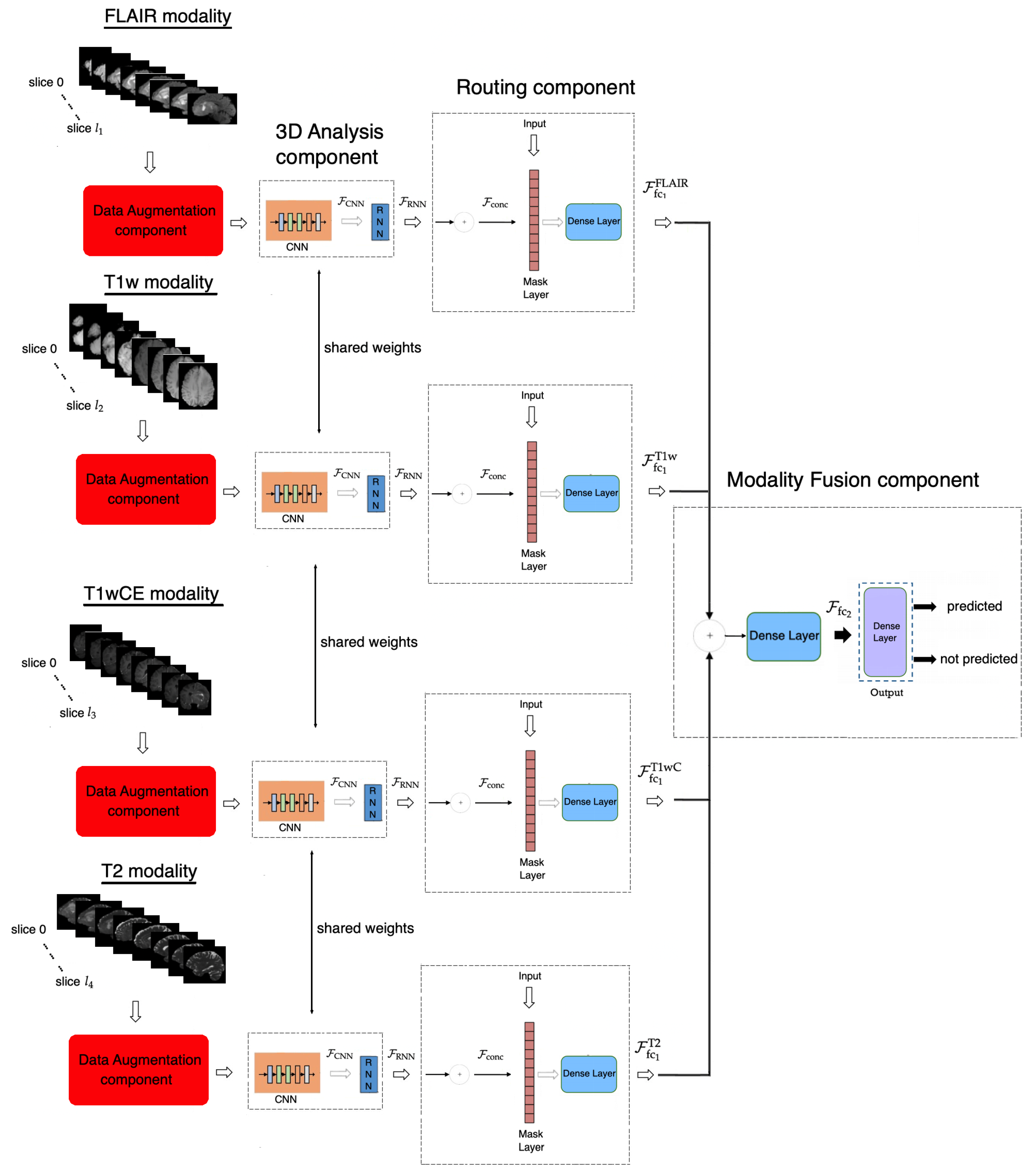
3.1. Proposed Method

First, all input 3D volumes for each modality (FLAIR, T1w, T1wCE, and T2) are fed to the data augmentation component. During training, this component applies a series of geometric transformations to the inputs and then performs a novel augmentation technique (MixAugment [22]) on them. During testing, this component applies test-time data augmentation [13] to the inputs.

Then, all input 3D transformed volumes for each modality (FLAIR, T1w, T1wCE, and T2) are padded with black slices to have lengths $t_1,t_2,t_3,t_4$ (e.g., each input FLAIR volume consists of $t_1$ slices, whereas each input T1w volume consists of $t_2$ slices). Each input 3D volume is first fed to the 3D analysis component. This component consists of a CNN [23], which performs local (per 2D image/slice) analysis, extracting features from each slice. Then, these features are fed to an RNN [24], which is placed on top of the CNN, to capture their temporal dependencies. The CNN and RNN networks perform global (per 3D volume) analysis. The RNN output features are then fed to the routing component, where they are concatenated and fed to a mask layer. This step is essential since we have annotations at the volume level (not at the slice level) and thus we know that all slices (not just independent slices) may convey important information for the final prediction of the network. This step is also important as it is the mask layer that dynamically selects RNN outputs, taking into account the input length, i.e., the ‘true’ number of slices of the currently analyzed volume. The output of the mask layer is then fed to a dense layer, which is equipped with batch normalization [14] and a GELU [15].

It should be noted that the above-described procedure is followed for each modality. For example, the input 3D FLAIR volume is fed to the 3D analysis component. Similarly, the input 3D T1 volume is fed to the 3D analysis component that is identical and shares the same weights with the corresponding component that the FLAIR modality was fed to. Then, the output of the 3D analysis component of the FLAIR modality is fed to the routing component. Likewise, the output of the 3D analysis component of the T1 modality is fed to the routing component, which is identical and shares the same weights with the corresponding component of the FLAIR modality.

The output features of the routing component for each modality are fed to the modality fusion component. The output features are concatenated and fed to a dense layer that maps them to the same feature space. Finally, the output layer follows, providing the final classification. In the following, we explain each component of our proposed method in more detail. Figure 1 provides an overview of our proposed framework, BTDNet.

3.1.1. Data Augmentation Component

During training, when batches of 3D volumes (X) are sampled (i.e., all slices within the 3D volumes are sampled), initially, we perform geometric transformations such as random horizontal flip and rotation and create transformed batches of 3D volumes ($T_X$). It should be noted that we do not perform the same geometric transformation on all slices within the same volume. On the contrary, we apply a different geometric transformation to each slice of the same volume (e.g., one slice is augmented with horizontal flip and 10° rotation, whereas its following slice is augmented only with −4° rotation).

Then, we apply MixAugment [22] to these transformed batches of 3D volumes. MixAugment is a simple and data-agnostic data augmentation routine that trains a method on convex combinations of pairs of examples and their labels. It extends the training distribution by incorporating the prior knowledge that linear interpolations of feature vectors should lead to linear interpolations of the associated targets. Therefore, it acts as a regularizer to favor linear behavior in-between training examples and it improves the generalization ability of the network, which is always a real-world challenge that can hinder the applicability and effectiveness of any method. We extend MixAugment to construct virtual training examples/3D volumes $(\tilde{X},\tilde{y})$ (one for each modality), and the method is trained concurrently on both real (r) and virtual (v) examples/3D volumes. The virtual examples, e.g., the FLAIR modality, are constructed as follows (similarly, virtual examples are constructed for the other modalities):

$$\begin{array}{cc}\hfill \tilde{X}& \hfill =\lambda T_{X_i}+(1-\lambda )T_{X_j}\hfill \\ \hfill \tilde{y}& \hfill =\lambda y_i+(1-\lambda )y_j\hfill \end{array}$$

(1)

where $T_{X_i}\in {\mathcal{R}}^{H\times W\times t_1}$ and $T_{X_j}\in {\mathcal{R}}^{H\times W\times t_1}$ are two random FLAIR modality inputs (i.e., 3D volumes). H and W are the height and width of each slice (i.e., 2D image); $t_1$ is the total number of slices within the volume after padding; $y_i$ and $y_j$$\in {\{0,1\}}^2$ are their corresponding one-hot labels; and $\lambda \sim \mathrm{B}(\alpha ,\alpha )\in [0,1]$ (i.e., Beta distribution) for $\alpha \in (0,\infty )$.

During inference, we apply test-time data augmentation [13]. For a given input 3D volume ($X_i$), we create three transformed versions: (i) one where only horizontal flip is performed ($F_{X_i}$); (ii) one where random rotation is performed ($R_{X_i}$); and (iii) one where both horizontal flip and random rotation are performed ($F{R}_{X_i}$). We feed these three versions, along with the non-augmented 3D volume, to the method, which generates a prediction for each version ($p^{F_{X_i}},p^{R_{X_i}},p^{F{R}_{X_i}},p^{X_i}$, respectively). The final prediction ($p_{\mathrm{final}}$) is the sum of these four outputs ($p_{\mathrm{final}}=p^{F_{X_i}}+p^{R_{X_i}}+p^{F{R}_{X_i}}+p^{X_i}$). It should be noted that we use the logits rather than the probabilities.

3.1.2. Three-Dimensional Analysis Component

mpMRI 3D volumes consist of 2D slices. CNNs are excellent for capturing local features, patterns, and structures in an image, making them well suited for extracting meaningful information from individual slices in a 3D MRI volume. By applying 2D convolutions across each slice, the CNN can effectively extract important spatial features from the MRI data. In medical imaging, the spatial context of features is often crucial. MRI scans contain anatomical structures and patterns that may extend across multiple slices. RNNs can capture the spatial dependencies and temporal information within the volume (by analyzing the extracted CNN features from each slice). This allows the method to consider the relationships between slices and how they evolve through the z-axis, which is important for understanding structures or changes/abnormalities over time. This is the aim of the 3D analysis component, which we describe in more detail below.

After all input 3D volumes for each modality (FLAIR, T1w, T1wCE, and T2) have been transformed and then padded to have lengths $t_1,t_2,t_3,t_4$, a CNN is applied to each of their slices, performing local (per 2D image/slice) analysis and extracting features from each slice. For example, in the case of a slice from a 3D input volume in the FLAIR modality, the extracted features from the CNN are denoted as ${\mathcal{F}}_{\mathrm{CNN}}\in {\mathcal{R}}^{H\times W\times D}$, with W, H, and D being the feature map’s width, height, and depth, respectively. Then, these features are fed to an RNN, which is placed on top of the CNN, to capture the temporal information and dependencies between consecutive slices within the same volume (for each modality). The RNN analyzes the features of the whole volume sequence, sequentially moving from slice 0 to slice $t_1$ if the input volume is for the FLAIR modality (and similarly for the other modalities). As shown in Figure 1, we obtain RNN features corresponding to each slice from 0 to $t_1$. For example, for a slice from a 3D input volume in the FLAIR modality, the extracted features from the RNN are denoted as ${\mathcal{F}}_{\mathrm{RNN}}\in {\mathcal{R}}^V$, with V being the feature vector that is outputted by the RNN. Thus, for the whole 3D input volume in the FLAIR modality, the extracted features from the RNN are denoted as ${\mathcal{F}}_{\mathrm{RNN}}\in {\mathcal{R}}^{V\times t_1}$. These RNN features are then fed to the routing component, which is described below. In total, the CNN plus RNN performs global (per 3D volume) analysis.

3.1.3. Routing Component

In this component, initially, the RNN features corresponding to the whole input 3D volume are concatenated since our target is the prediction of the MGMT promoter methylation status using the whole volume, similar to the annotations provided in the utilized dataset. The concatenated features (${\mathcal{F}}_{\mathrm{conc}}\in {\mathcal{R}}^{V·t_1}$) are then fed to the mask layer. The original (before padding) length $l_1$ of the input FLAIR volume (similarly, $l_2,l_3,$ and $l_4$ for the T1w, T1wCE, and T2 volumes) is transferred from the input to the mask layer to inform the routing process. During model training, the routing mechanism dynamically selects the RNN outputs, selecting as many of them as indicated by the length l of the input volume, keeping their values while setting the values of the remaining RNN outputs to zero. Therefore, only the selected outputs are routed into the subsequent dense layer.

This dense layer is equipped with batch normalization and a GELU. We use the GELU due to its advantages over the ReLU and its variants. The dense layer learns to extract high-level information from the concatenated RNN outputs. During training, we only update the weights that connect the dense layer neurons with the RNN outputs routed in the concatenated vector by the mask layer. The remaining weights are updated whenever (i.e., in another input volume) respective RNN outputs are selected in the concatenated vector by the mask layer. Objective function minimization is performed, as in networks with dynamic routing, by keeping the weights that do not participate in the routing process constant and ignoring links that correspond to non-routed RNN outputs. Finally, the output of the dense layer (${\mathcal{F}}_{{\mathrm{fc}}_1}\in {\mathcal{R}}^{V^{\prime }}$) is fed to the modality fusion component, as explained below.

3.1.4. Modality Fusion Component

Initially, the output features of the dense layer in the FLAIR modality ${\mathcal{F}}_{{\mathrm{fc}}_1}^{\mathrm{FLAIR}}\in {\mathcal{R}}^{V^{\prime }}$ are concatenated with the corresponding output features of the dense layer for the other modalities: T1w, T1wCE, and T2 (${\mathcal{F}}_{{\mathrm{fc}}_1}^{\mathrm{T}1\mathrm{w}}\in {\mathcal{R}}^{V^{\prime }}$, ${\mathcal{F}}_{{\mathrm{fc}}_1}^{\mathrm{T}1\mathrm{wCE}}\in {\mathcal{R}}^{V^{\prime }}$, and ${\mathcal{F}}_{{\mathrm{fc}}_1}^{\mathrm{T}2}\in {\mathcal{R}}^{V^{\prime }}$), respectively. These features have already been normalized in the routing component, where batch normalization was performed on the dense layers’ outputs for each modality; therefore, features coming from different modalities are all within the same range. The concatenated features are then fed to another dense layer (${\mathcal{F}}_{{\mathrm{fc}}_2}\in {\mathcal{R}}^{V^{\prime \prime }}$) equipped with a GELU that maps them to the same feature space. This step is important, as leveraging and fusing information from multiple modalities helps the method to have a richer data representation, reduce redundancy and ambiguity in the data interpretation, and mitigate data scarcity. Finally, the output layer follows, which consists of two units, generating the final classification for the MGMT promoter methylation status.

3.1.5. Objective Function

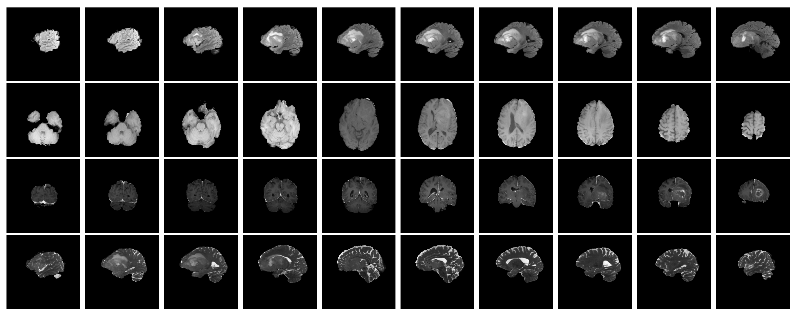
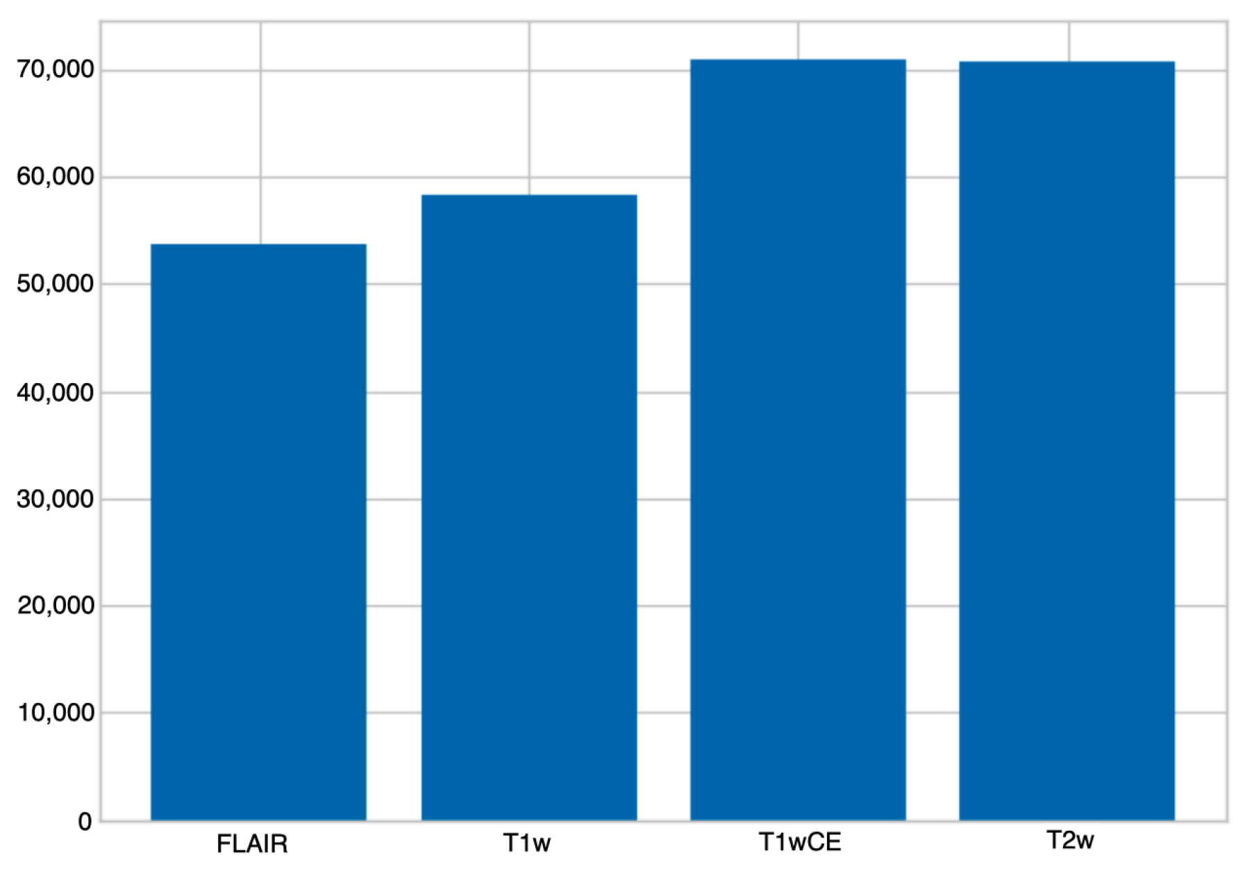
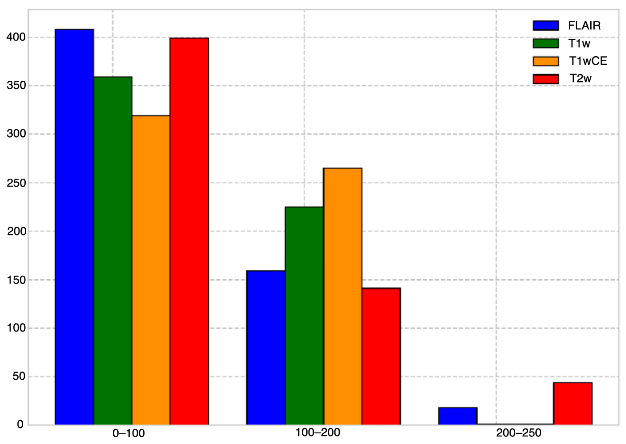
For the objective function, we built upon the focal loss (FL) [16] for multi-class classification, which is defined as follows:

$$\begin{array}{cc}\hfill & \hfill {\mathcal{L}}_{FL}=\sum _{i=1}^{batch}\left[-\alpha {(1-p)}^{\gamma }\log p-(1-\alpha )p^{\gamma }\log (1-p)\right],\hfill \end{array}$$

(2)

where p is the method’s estimated probability for the positive class; $\alpha$ balances the importance of positive/negative examples; and ${(1-p)}^{\gamma }$ and $p^{\gamma }$ are modulating factors that reduce the loss contribution from easy examples and extend the range in which an example receives low loss. These modulating factors consist of the tunable focusing parameter $\gamma \ge 0$, which smoothly adjusts the rate at which easy examples are down-weighted.

As explained in the MixAugment strategy above, in each training iteration, the method is fed with both $T_{X_i}$ and $T_{X_j}$, as well as the constructed virtual volume $\tilde{X}$ (from Equation (1)). Therefore, the overall objective function consists of the sum of the focal losses for the real (r) and virtual (v) volumes:

$$\begin{array}{cc}\hfill & \hfill {\mathcal{L}}_{total}={\mathcal{L}}_{FL}^v+{\mathcal{L}}_{FL}^{r_i}+{\mathcal{L}}_{FL}^{r_j}\hfill \end{array}$$

(3)

3.2. Dataset

The RSNA-MICCAI consortium developed a dataset [17] that comprises multi-parametric magnetic resonance imaging (mpMRI) scans (i.e., 3D volumes) from various institutions, annotated for the prediction of a specific genetic characteristic of glioblastoma, namely the MGMT promoter methylation status. Each mpMRI scan consists of four modalities: fluid-attenuated inversion recovery (FLAIR), T1-weighted pre-contrast (T1w), T1-weighted post-contrast (T1wCE), and T2-weighted (T2). Each of these modalities offers a specific imaging perspective. For instance, the FLAIR modality provides post-cerebrospinal fluid suppression imagery, where fluidic signals such as water are muted to emphasize other components. Figure 2 shows some slices of each modality from the same mpMRI scan. Each modality contains a varying number of slices. Figure 3 illustrates the total number of slices of each modality for all mpMRI scans. In total, the dataset comprises 585 labeled samples, each with dimensions of $512\times 512$.

3.3. Pre-Processing

Initially, we performed segmentation of each slice of all mpMRI scans (across all modalities) to detect the brain regions and crop them. We used a simple technique for segmentation that exploited the fact that each slice consisted of the brain on a black background. Each slice was scanned from top to bottom and from left to right and vice versa in order to find the location (i.e., the coordinates) of the first non-black pixel. We then aggregated all these locations and extracted only the four that defined the bounding box we created. We then cropped each 2D slice according to its corresponding bounding box. Additionally, we removed some slices, mainly at the start and end of the MRI scan sequence of slices, since these slices displayed only a minuscule portion of the brain or were entirely void of any useful content. To determine this, we checked whether a slice had a bounding box with an area less than 5% of the total area of the whole slice; if such cases were found, the corresponding slices were removed. Figure 4 shows the total number of remaining slices within each mpMRI scan (for each modality). Finally, all segmented slices were resized to a resolution of $224\times 224\times 3$ pixels, and their intensity values were normalized to $[-1,1]$. The resulting segmented slices constitute the input to our method.

3.4. Performance Metrics

The performance measure employed was the average $F_1$ score across the two categories (i.e., macro $F_1$ score):

$$\mathcal{P}=\frac{{\sum }_{expr}{F}_1^{expr}}{2}$$

(4)

The $F_1$ score [25] is a weighted average of the recall (i.e., the ability of the classifier to find all the positive samples) [26] and precision (i.e., the ability of the classifier not to label a sample as positive when it is actually negative) [25]. The $F_1$ score takes values in the range of $[0,1]$, and high values are desired. The $F_1$ score is defined as:

$$F_1=\frac{2\times precision\times recall}{precision+recall}$$

(5)

3.5. Implementation Details

We used ResNet18 [18] (discarding the output layer but keeping the global average pooling) as the CNN, and a single one-directional LSTM [24] consisting of 128 units as the RNN. The dense layer in the routing component consisted of 64 hidden units, and the dense layer in the modality fusion component consisted of 128 hidden units. We used a batch size of 4 (we also experimented with values of 2, 6, 8, 16, and 32, but they all resulted in poor performance). We set the lengths $t_1$ and $t_4$ (corresponding to the FLAIR and T2 modalities, respectively) to 250, and the lengths $t_2$ and $t_3$ (corresponding to the T1w and T1wCE modalities, respectively) to 200.

We used stratified fivefold cross-validation. The training was divided into two phases: first, each modality stream/subnetwork was trained independently, and then the multimodal method was trained end-to-end. We utilized SGD with a momentum of 0.9 [27] and SAM [28] optimizers (we also experimented with the ADAM optimizer and RMSprop, but they both generated poor results). The learning rate was set to ${10}^{-4}$ for training from scratch and ${10}^{-5}$ for end-to-end training (we also used learning rates of ${10}^{-2}$, ${10}^{-3}$, and ${10}^{-5}$ for training from scratch, and learning rates of ${10}^{-3}$, ${10}^{-4}$, and ${10}^{-6}$ for end-to-end training, but these resulted in poor performance in all cases). The training was performed on a Tesla V100 32 GB GPU.

4. Experimental Results

This section describes the set of experiments conducted to evaluate the performance of the proposed approach. First, we compare the performance of BTDNet with that of the state-of-the-art methods that participated in the RSNA-ASNR-MICCAI BraTS 2021 Challenge. We show that it outperforms these methods by large margins. Finally, we perform ablation studies that illustrate the contribution of the various components of BTDNet. In particular, we focus on the 3D analysis component (i.e., the choice of CNN and RNN models); routing component (i.e., the existence of the mask layer, as well as the number of hidden units in the dense layer); contribution of each modality; data augmentations (geometric transformations, MixAugment and test-time data augmentation); and the objective function.

4.1. Comparison with the State-of-the-Art

First, we compare the performance of BTDNet to that of the state-of-the-art methods: the unimodal 3D-Resnet10-Trick [8] (winner of the RSNA-ASNR-MICCAI BraTS 2021 Challenge), the multimodal EfficientNet-LSTM-mpMRI [10] (runner up in the challenge), the multimodal EfficientNet-Aggr [11] (third place in the challenge), the unimodal YOLO-EfficientNet [9] (fourth place in the challenge), and the multimodal stats-EfficientNet [12] (fifth place in the challenge). For a fair comparison with our method, which utilized segmented 3D volumes, we re-implemented these methods and also utilized the same segmented data.

Table 1. Comparison between BTDNet and the state-of-the-art on the RSNA-ASNR-MICCAI BraTS 2021 Challenge dataset.

Methods	${\mathit{F}}_1$ Score
stats-EfficientNet [12]	42.9 ± 6.84
YOLO-EfficientNet [9]	44.4 ± 7.41
EfficientNet-Aggr [11]	46.1 ± 4.68
EfficientNet-LSTM-mpMRI [10]	47.4 ± 4.41
3D-Resnet10-Trick [8]	62.9 ± 4.8
BTDNet	66.2 ± 3.1

shows the performance of the state-of-the-art methods and our method. The results are presented in the form of an average of five folds ± spread (i.e., difference between max. and min. performance within the five folds). It can be seen in Table 1 that our method outperformed all the other state-of-the-art methods by large margins. In more detail, it outperformed the winner of the challenge, 3D-Resnet10-Trick, by 3.3%, and it outperformed all other methods by at least 18.8%. Table 1 also shows that our method achieved the minimum spread among all the state-of-the-art methods.

It should be noted that all the state-of-the-art methods utilized an ad hoc strategy of selecting a fixed input length by removing or duplicating slices within each 3D volume. Furthermore, some methods utilized CNN-RNN architectures, in which the 3D volume annotation was propagated to each slice within the volume. Finally, we performed an extra experiment, which is not shown in Table 1 so as not to clutter the results. In more detail, we implemented 3D-Resnet10-Trick (winner of the challenge) and utilized non-segmented data. Surprisingly, we noticed that the method’s performance increased from $62.9\pm 4.8$ (which was the case when segmented data were used) to $63.3\pm 4.4$. This indicates that the method focused more on regions outside of the brain, which played a role in the increase in performance (however, this is not correct, as the MGMT promoter methylation status exists in the brain region and should be predicted only from that region).

4.2. Ablation Study

In the following, we perform various ablation experiments to evaluate the contribution of each novel component of BTDNet. First, we utilized different backbone networks to act as the CNN in the 3D analysis component of BTDNet. We experimented with using ResNet50 and ResNet101 (which are larger networks than ResNet18, which was chosen as the CNN in BTDNet), EfficientNetB0 and EfficientNetB3 (which have been used by state-of-the-art methods and proven their value), and ConvNeXt-T [29]. As can be seen in

Table 2. Ablation study evaluating the contribution of each component of BTDNet on the RSNA-ASNR-MICCAI BraTS 2021 Challenge dataset.

BTDNet	${\mathit{F}}_1$ Score
ResNet50 as CNN	64.1 ± 3.6
ResNet101 as CNN	62.8 ± 3.88
EfficientNetB0 as CNN	63.9 ± 3.92
EfficientNetB3 as CNN	62.9 ± 4.21
ConvNeXt-T as CNN	64.9 ± 3.7
LSTM, 64 units as RNN	65.1 ± 3.5
LSTM, 256 units as RNN	64.3 ± 4.3
GRU, 64 units as RNN	65 ± 3.7
GRU, 256 units as RNN	64.4 ± 4.4
no routing component	60.9 ± 5.7
no mask layer	62.9 ± 5.2
dense layer (routing component), 32 units	65.1 ± 3.4
dense layer (routing component), 128 units	64.9 ± 3.6
only FLAIR modality	64.5 ± 3.3
only T1w modality	63.2 ± 4.3
only T1wCE modality	63.8 ± 4.1
only T2 modality	64.1 ± 3.8
no test-time data augmentation	65.2 ± 3.4
no geometric transformations	65.3 ± 3.3
no MixAugment	64.7 ± 3.8
categorical cross-entropy as objective function	64.9 ± 3.4
binary cross-entropy as objective function	64.5 ± 3.5
BTDNet	66.2 ± 3.1

, ResNet18 is a better backbone CNN than its larger counterparts (ResNet50 and ResNet101). We can see that the larger the ResNet network becomes (and the more layers it has), the lower the performance. This probably occurs due to the small size of the training dataset; larger models are too complex to model. This also occurred in the case of the EfficientNet models, as the performance of EfficientNetB0 surpassed that of EfficientNetB3. Table 2 also illustrates that the performance of ConvNeXt-T surpassed that of ResNet50, which was expected. Finally, the overall best performance was achieved when ResNet18 was utilized. As a second ablation experiment, we utilized different networks to act as the RNN in the 3D analysis component of BTDNet. We experimented with using LSTM and GRU, varying their numbers of units from 64 to 128 and 256. As can be seen in Table 2, LSTM and GRU achieved similar performance. The best results were obtained when LSTM with 128 units was used. If the number of units increased, the performance of the method started to decrease.

Next, we assessed the contribution of the routing component and its subcomponents. In more detail, we experimented with not using the routing component at all or without using the mask layer. Thus, our method addressed the problem of different lengths in each volume using a traditional ad hoc strategy, either by removing slices when a larger length was encountered or duplicating slices when the volume contained fewer slices. Table 2 proves that these approaches did not yield good results. Our method outperformed them by large margins (at least 3.3%), as was the case with the state-of-the-art methods that used such ad hoc strategies. This was expected, as the removal of slices resulted in the loss of important information for the final decision, and the duplication of slices negatively affected the final decision, biasing the method toward the repeating data and thus toward one category. We further experimented with using different numbers of hidden units in the dense layer of the routing component by experimenting with 32, 64, and 128 units. The best results were obtained when we used 64 units.

In the following, we assess the contribution of each modality and thus the multimodal approach. Table 2 illustrates the results achieved using our method when employing a unimodal approach (either the FLAIR, T1w, T1wCE, or T2 modalities) and a multimodal approach (which utilizes all available modalities). One can see in Table 2 that for the unimodal methods, using the FLAIR modality resulted in the best performance. When the T2 modality was used, the second-best performance was achieved. When the T1wCE modality was used, it outperformed the case when the T1w was used. Table 2 shows that when the multimodal approach was used, it outperformed all unimodal approaches. This was expected, as different modalities provided complementary information. By incorporating multiple modalities, our method could access a richer and more diverse set of data, leading to a more comprehensive understanding of the targeted problem. Additionally, our multimodal method likely reduced redundancy and ambiguity in the data interpretation, becoming more robust and less susceptible to errors or noise. Finally, in some cases, where there were limited data available in a single modality, the multimodal approach helped mitigate data scarcity issues by leveraging information from other modalities.

In the following, we perform an ablation study with regard to the proposed data augmentation strategies. In more detail, Table 2 shows the performance of our method when (i) no test-time data augmentation was performed (i.e., during inference, the method was evaluated only on the real non-augmented data, and three augmented versions of the data were not created and used in the evaluation); (ii) no geometric transformations were used (i.e., both random horizontal flip and rotation were not performed on the data during training); and (iii) no MixAugment was used (i.e., the method was trained only using the real training data and during training, no virtual data were constructed and subsequently used along with the real data). It can be seen that in all cases, the performance of our method decreased, verifying that each data augmentation strategy alone resulted in a performance gain, and the best performance was achieved when all were used together. The biggest decrease in performance was observed when the MixAugment strategy was not used. It should also be noted that we performed one more experiment that is not shown so as not to clutter the results. We performed only geometric transformations (i.e., random horizontal flip and rotation), and the same transformation was performed on the slices within the same volume. Our method’s performance in this case was 0.8% lower than its corresponding performance when a different random geometric transformation was performed on the slices within the same volume.

Finally, the last ablation experiment concerns the contribution of the objective function. We experimented with using the proposed multi-class focal loss, as well as the standard categorical cross-entropy (with two outputs in the method) and binary cross-entropy (with one output in the method) losses. Table 2 shows that when the multi-class focal loss was utilized, our method achieved the best performance, which was at least 1.3% higher than the corresponding results when the other losses were used.

5. Conclusions and Future Work

In this paper, we proposed BTDNet, a new multimodal approach that harmonizes the analysis of 3D image volumes consisting of different numbers of slices and annotations per volume. In more detail, BTDNet accepts as input an mpMRI (i.e., a FLAIR 3D volume, T1w 3D volume, T1wCE 3D volume, and T2 3D volume) and predicts the MGMT promoter methylation status. BTDNet consists of four components: 3D analysis, the routing, the modality fusion, and the data augmentation.

When BTDNet is fed with a new 3D volume input, a CNN performs the initial local (per 2D image/slice) analysis, extracting features from each slice. Then, these features are fed to an RNN and placed on top of the CNN to capture their temporal dependencies. The CNN and RNN networks perform global (per 3D volume) analysis. The RNN output features are then concatenated and fed to a mask layer, which dynamically selects RNN outputs, taking into account their input length. The output of the mask layer is then fed to a dense layer. This procedure is followed for each of the four modalities; the output features of the dense layer for each modality are then concatenated and fed to a dense layer that maps them to the same feature space. Finally, the output layer follows providing the final classification. The objective function for training BTDNet is based on the focal loss for multi-class classification.

Excellent performance was achieved on the dataset of the RSNA-ASNR-MICCAI BraTS 2021 Challenge, verifying our developments and surpassing all state-of-the-art methods by large margins. In more detail, BTDNet outperformed the winning method of the challenge by 3.3% and the other top-four methods by 18.8–23.3% in terms of the F1 score. Finally, an extensive ablation study was conducted and presented, validating the contribution and performance gain that each component of BTDNet brings.

It should be noted that in order for our method to be used in real-life clinical situations, a much larger and more diverse dataset will need to be used for training BTDNet, and clinical trials should be conducted.

The hypothesis and limitation of our method is the assumption that all modalities are available and present. An interesting future direction could be to extend BTDNet to work in the case of one or multiple missing modalities. Another future direction could be to develop a joint method that initially performs brain and tumor segmentation and then predicts the MGMT promoter methylation status. This new method could be built upon BTDNet. Finally, our work only considered the temporal dependencies between data of the same modality, and the relationship between data of different modalities was not investigated. This inter-modality relation could be another intriguing future direction.

References

1. Shergalis, A.; Bankhead, A.; Luesakul, U.; Muangsin, N.; Neamati, N. Current challenges and opportunities in treating glioblastoma. Pharmacol. Rev. 2018, 70, 412–445. [Google Scholar] [CrossRef] [PubMed]
2. McKinnon, C.; Nandhabalan, M.; Murray, S.A.; Plaha, P. Glioblastoma: Clinical presentation, diagnosis, and management. BMJ 2021, 374, n1560. [Google Scholar] [CrossRef] [PubMed]
3. Thawani, R.; McLane, M.; Beig, N.; Ghose, S.; Prasanna, P.; Velcheti, V.; Madabhushi, A. Radiomics and radiogenomics in lung cancer: A review for the clinician. Lung Cancer 2018, 115, 34–41. [Google Scholar] [CrossRef] [PubMed]
4. Jansen, R.W.; van Amstel, P.; Martens, R.M.; Kooi, I.E.; Wesseling, P.; de Langen, A.J.; Menke-Van der Houven, C.W.; Jansen, B.H.; Moll, A.C.; Dorsman, J.C.; et al. Non-invasive tumor genotyping using radiogenomic biomarkers, a systematic review and oncology-wide pathway analysis. Oncotarget 2018, 9, 20134. [Google Scholar] [CrossRef] [PubMed]
5. Villanueva-Meyer, J.E.; Mabray, M.C.; Cha, S. Current clinical brain tumor imaging. Neurosurgery 2017, 81, 397. [Google Scholar] [CrossRef] [PubMed]
6. Rivera, A.L.; Pelloski, C.E.; Gilbert, M.R.; Colman, H.; De La Cruz, C.; Sulman, E.P.; Bekele, B.N.; Aldape, K.D. MGMT promoter methylation is predictive of response to radiotherapy and prognostic in the absence of adjuvant alkylating chemotherapy for glioblastoma. Neuro-Oncology 2010, 12, 116–121. [Google Scholar] [CrossRef] [PubMed]
7. Louis, D.N.; Perry, A.; Reifenberger, G.; Von Deimling, A.; Figarella-Branger, D.; Cavenee, W.K.; Ohgaki, H.; Wiestler, O.D.; Kleihues, P.; Ellison, D.W. The 2016 World Health Organization classification of tumors of the central nervous system: A summary. Acta Neuropathol. 2016, 131, 803–820. [Google Scholar] [CrossRef] [PubMed]
8. Baba, F. RSNA-MICCAI Brain Tumor Radiogenomic Classification. 2021. Available online: https://www.kaggle.com/competitions/rsna-miccai-brain-tumor-radiogenomic-classification/discussion/281347 (accessed on 29 October 2023).
9. Roberts, D. RSNA-MICCAI Brain Tumor Radiogenomic Classification. 2021. Available online: https://www.kaggle.com/competitions/rsna-miccai-brain-tumor-radiogenomic-classification/discussion/280033 (accessed on 29 October 2023).
10. Phan, M. RSNA-MICCAI Brain Tumor Radiogenomic Classification. 2021. Available online: https://www.kaggle.com/competitions/rsna-miccai-brain-tumor-radiogenomic-classification/discussion/280029 (accessed on 29 October 2023).
11. Soares, C. RSNA-MICCAI Brain Tumor Radiogenomic Classification. 2021. Available online: https://www.kaggle.com/competitions/rsna-miccai-brain-tumor-radiogenomic-classification/discussion/287713 (accessed on 29 October 2023).
12. Tangirala, B. RSNA-MICCAI Brain Tumor Radiogenomic Classification. 2021. Available online: https://www.kaggle.com/competitions/rsna-miccai-brain-tumor-radiogenomic-classification/discussion/281911 (accessed on 29 October 2023).
13. Radosavovic, I.; Dollár, P.; Girshick, R.; Gkioxari, G.; He, K. Data distillation: Towards omni-supervised learning. In Proceedings of the IEEE Conference on Computer Vision and Pattern Recognition, Salt Lake City, UT, USA, 18–23 June 2018; pp. 4119–4128. [Google Scholar]
14. Santurkar, S.; Tsipras, D.; Ilyas, A.; Madry, A. How does batch normalization help optimization? Adv. Neural Inf. Process. Syst. 2018, 31. [Google Scholar]
15. Hendrycks, D.; Gimpel, K. Gaussian error linear units (gelus). arXiv 2016, arXiv:1606.08415. [Google Scholar]
16. Lin, T.Y.; Goyal, P.; Girshick, R.; He, K.; Dollár, P. Focal loss for dense object detection. In Proceedings of the IEEE International Conference on Computer Vision, Venice, Italy, 22–29 October 2017; pp. 2980–2988. [Google Scholar]
17. Baid, U.; Ghodasara, S.; Mohan, S.; Bilello, M.; Calabrese, E.; Colak, E.; Farahani, K.; Kalpathy-Cramer, J.; Kitamura, F.C.; Pati, S.; et al. The rsna-asnr-miccai brats 2021 benchmark on brain tumor segmentation and radiogenomic classification. arXiv 2021, arXiv:2107.02314. [Google Scholar]
18. He, K.; Zhang, X.; Ren, S.; Sun, J. Deep residual learning for image recognition. In Proceedings of the IEEE Conference on Computer Vision and Pattern Recognition, Las Vegas, NV, USA, 26 June–1 July 2016; pp. 770–778. [Google Scholar]
19. Tan, M.; Le, Q. Efficientnet: Rethinking model scaling for convolutional neural networks. In Proceedings of the International Conference on Machine Learning, PMLR, Long Beach, CA, USA, 9–15 June 2019; pp. 6105–6114. [Google Scholar]
20. Hochreiter, S.; Schmidhuber, J. Long short-term memory. Neural Comput. 1997, 9, 1735–1780. [Google Scholar] [CrossRef] [PubMed]
21. Jocher, G. YOLOv5 by Ultralytics. Zenodo 2020. [Google Scholar] [CrossRef]
22. Psaroudakis, A.; Kollias, D. Mixaugment & mixup: Augmentation methods for facial expression recognition. In Proceedings of the IEEE/CVF Conference on Computer Vision and Pattern Recognition, New Orleans, LA, USA, 18–24 June 2022; pp. 2367–2375. [Google Scholar]
23. LeCun, Y.; Bengio, Y. Convolutional networks for images, speech, and time series. Handb. Brain Theory Neural Netw. 1995, 3361, 1995. [Google Scholar]
24. Gers, F.A.; Schmidhuber, J.; Cummins, F. Learning to forget: Continual prediction with LSTM. Neural Comput. 2000, 12, 2451–2471. [Google Scholar] [CrossRef] [PubMed]
25. Powers, D.M. Evaluation: From precision, recall and F-measure to ROC, informedness, markedness and correlation. arXiv 2020, arXiv:2010.16061. [Google Scholar]
26. Schütze, H.; Manning, C.D.; Raghavan, P. Introduction to Information Retrieval; Cambridge University Press: Cambridge, UK, 2008; Volume 39. [Google Scholar]
27. Amari, S. Backpropagation and stochastic gradient descent method. Neurocomputing 1993, 5, 185–196. [Google Scholar] [CrossRef]
28. Foret, P.; Kleiner, A.; Mobahi, H.; Neyshabur, B. Sharpness-aware minimization for efficiently improving generalization. arXiv 2020, arXiv:2010.01412. [Google Scholar]
29. Liu, Z.; Mao, H.; Wu, C.Y.; Feichtenhofer, C.; Darrell, T.; Xie, S. A convnet for the 2020s. In Proceedings of the IEEE/CVF Conference on Computer Vision and Pattern Recognition, New Orleans, LA, USA, 18–24 June 2022; pp. 11976–11986. [Google Scholar]
Figure 1. The proposed multimodal BTDNet takes as input mpMRI 3D volumes (FLAIR, T1w, T1wCE, and T2 modalities). BTDNet consists of the following components: (i) data augmentation (geometric transformations, adapted MixAugment, test-time data augmentation); (ii) 3D analysis (CNN plus RNN); (iii) routing (mask layer, routing, dense layer); and (iv) modality fusion (dense layer, output layer). The symbol ‘+’ in a circle denotes the concatenation operation.
Applsci 13 11984 g001
Figure 2. Example of a whole mpMRI scan, where one can see some slices from the FLAIR modality (top row); T1w modality (second row); T1wCE modality (third row); and T2 modality (bottom row).
Applsci 13 11984 g002
Figure 3. The total number of slices of each modality for all mpMRI scans.
Applsci 13 11984 g003
Figure 4. The total number of slices for each modality within each mpMRI scan.
Applsci 13 11984 g004