Application of Physics-Informed Neural Networks to River Silting Simulation

Abstract

Water resource pollution, particularly in river channels, presents a grave environmental challenge that necessitates a comprehensive and systematic approach encompassing assessment, forecasting, and effective management. This article provides a comprehensive exploration of the methodology and modeling tools employed to scrutinize the process of river channel pollution due to silting, rooted in the fundamental principles of hydrodynamics and pollutant transport dynamics. The study’s methodology seamlessly integrates numerical simulations with state-of-the-art neural network techniques, with a specific focus on the physics-informed neural network (PINN) method. This innovative approach represents a groundbreaking fusion of artificial neural networks (ANNs) and physical equations, offering a more efficient and precise means of modeling a wide array of complex processes and phenomena. The proposed mathematical model, grounded in the Euler equation, has been meticulously implemented using the Ansys Fluent software package, ensuring accuracy and reliability in the computations. In a pivotal phase of the research, a thorough comparative analysis was conducted between the results derived using the PINN method and those obtained using conventional numerical approaches with the Ansys Fluent software package. The outcomes of this analysis revealed the superior performance of the PINN method, characterized by the generation of smoother pressure fluctuation profiles and a significantly reduced computation time, underscoring its potential as a transformative modeling tool. The calculated data originating from this study assume paramount significance in the ongoing battle against river sedimentation. Beyond this immediate application, these findings also serve as a valuable resource for creating predictive materials pertaining to river channel silting, thereby empowering decision-makers and environmental stakeholders with essential information. The utilization of modeling techniques to address pollution concerns in river channels holds the potential to revolutionize risk management and safeguard the integrity of our vital water resources. However, it is imperative to underscore that the effectiveness of such models hinges on ongoing monitoring and frequent data updates, ensuring that they remain aligned with real-world conditions. This research not only contributes to the enhanced understanding and proactive management of river channel pollution due to silting but also underscores the pivotal role of advanced modeling methodologies in the preservation of our invaluable water resources for present and future generations.

1. Introduction

Sedimentation is one of the primary factors contributing to water pollution. Essentially, sedimentation refers to water pollution caused by the presence of solid particles, mainly composed of debris or clay particles (Zhang et al., 2021, [1]) (Hasan et al., 2023, [2]). Additionally, sedimentation processes can also occur as a result of land erosion or human activities in aquatic environments (Wu et al., 2023, [3]), (Liquan Sun et al., 2023, [4]).

A river that is a naturally self-organizing system regulated via the accumulation and transport of sedimentary materials such as clay, sand, silt, and gravel is called an alluvial river. The main sources of alluvial materials for the river are the erosion of soil, rock formations, and bank areas in the river basin. When the river carries these materials in water flows, they settle to the bottom of the channel and can change its shape and depth (Best and Darby, 2020, [5]), causing the topographical evolution of the river to deviate from its natural course (Marren et al., 2014, [6]). This deviation can further affect the various socio-economic functions performed by rivers, such as navigation, flood mitigation, and water supply. It follows from this that the river system should be considered a complex component of a single natural system. (Hawley, 2018, [7]; Merembayev, 2023, [8]).

River silting processes are extremely unstable (Constantine et al., 2014, [9]); they pose a serious threat to the life and property of people living in their floodplains, and can also harm infrastructure and the environment. The increased frequency of meteorological disasters leads to the fact that the risk of floods of these rivers may increase (Dottori et al., 2018, [10]). For example, severe silting of the Kosi and Indus rivers in South Asia led to the formation of ultra-high channels, resulting in dam failures in 2008 and 2010, respectively, causing severe damage to downstream residential areas (Sinha et al., 2019, [11]). For this reason, when modeling the prediction of the behavior of silty rivers, it is very important to take into account complex hydrodynamic processes (Philips et al., 2022, [12]). Thus, it is extremely important to be able to manage silty rivers because this problem is relevant not only to researchers but also to politicians and other stakeholders, and requires careful further study and consideration.

For a more detailed study of the described problem, it is necessary to conduct full-scale experiments (Powledge et al., 1989, [13]; Schmocker and Hager 2009, [14]), which make it possible to study the nature of the movement of the water flow and the sedimentary layer under various conditions, as well as based on real observations (Froehlich 2008, [15]). While real-world observations clearly demonstrate the problem, they are often poorly documented. Thus, numerous laboratory experiments were carried out to study the clogging of streams with silt particles (Fetzer et al., 2017, [16]; Yao et al., 2013, [17]; Kazidenov et al., 2023 [18]; Merembayev et al., 2023, [19]). However, large-scale real experiments on the silting process are not only extremely difficult to perform, but they also require huge resource costs. Often, the developed numerical algorithm is tested on the basis of experimental data (Ecemis, 2021, [20]; Narbayev et al., 2022, [21]; Omarova, P., Merembayev, T. et al., 2023, [22]). One study (Soares-Frazão et al., 2007, [23]) presents a laboratory experiment demonstrating the morphological changes in a river channel and destruction of river banks. The bottom and banks of the river channel consisted of homogeneous sand, and the cross-section of the experimental setup had the shape of a rectangular trapezoid. The article (Goutiere et al., 2011, [24]) demonstrates the behavior of the water flow in an expanding installation above a moving layer of homogeneous sand.

Most of the early research was based on numerical simulation methods; however, in the last decade, breakthroughs in computer vision (CV) (Buribayev et al., 2021, [25], Kenshimov et al. [26]) and natural language processing (NLP) have led to the rapid development of artificial neural networks (ANNs) (Yeleussinov et al. [27]). An ANN takes input (e.g., a series of images) and outputs a prediction based on the task (e.g., image recognition).

The quality of the forecast depends on the amount of information in the training data and on minimizing the error function when training the neural network. This opens up new possibilities in modeling physical phenomena, including drainage processes and river pollution. However, in fluid dynamics, there is often a lack of the experimental data necessary for training neural networks. Recently, a method called physics-based neural network (PINN) was introduced, which allows neural networks to be trained on random samples without observations (Sukumar and Srivastava, 2022, [28]). PINN represents a new approach to solving physics problems by allowing neural networks to assimilate physical laws during the learning process. This allows predictions to be made, taking into account the physical conditions of the problem. The PINN method can provide computational advantages, especially when accurate data are available. This article provides an overview of the methodology and tools for modeling river pollution and sedimentation processes based on the principles of hydrodynamics and pollutant transport. The study used numerical simulation and the PINN method to compare the results to identify the advantages of each method.

In this study, the task is to assess the indicators of velocity, pressure, and density in the aquatic environment for subsequent modeling of silting in river channels. Indicators are predicted using the modern approach of physics-informed neural networks. A comparative analysis of the simulation results with Ansys Fluent was also performed to determine the most optimal method in terms of computational speed and computational accuracy.

The methodology section elaborates on the utilization of physics-based neural networks and modeling techniques within the Ansys Fluent software package (ANSYS-FLUENT 2009, [29]), specifically addressing the Euler problem. Subsequently, the results section encompasses a presentation of the simulation outcomes obtained using physics-based neural networks and numerical simulation techniques in Ansys Fluent. The discussion section provides a concise summary of the methodologies employed and offers a brief examination of the findings.

2. Materials and Methods

2.1. Neural Networks Based on Physics

The physics-informed neural networks (PINN) method is extremely popular in fluid flow simulation, and numerous studies demonstrate the success of using this method (Meng et al., 2020, [30]; Cheng et al., 2021, [31]; Huang et al., 2023, [32]). However, free surface problems are a major problem for the PINN method in its original formulation. So far, studies on solving free surface flow problems using the PINN method are limited, and free surface problems have been solved only in the shallow water approximation (Holland, 2011, [33]), where all calculations are performed on the free surface (Ardakani and Bridges, 2010, [34]) and where the basic equations are simpler. Therefore, a PINN structure for solving the general problem of a free surface in rough water conditions is not available and, therefore, is very necessary.

The application of the PINN method to solving the Euler equations and detecting shock wave evolution is a complex task that requires a deep understanding of the physical processes, the creation of suitable training data, and network configuration.

Detecting shock wave evolution and solving the Euler equations using a physics-informed neural network (PINN) involves specific steps. The general procedure for implementing the PINN method is presented below:

• Definition of the physical problem: Begin by clearly defining the physical problem you want to solve. In your case, it involves the Euler equations describing gas dynamics and shock wave evolution.
• Formulation of the mathematical model: Translate the physical problem into a mathematical model. The Euler equations for gas dynamics constitute a system of hyperbolic equations. Solving this system of equations is essential for modeling shock wave evolution.
• Preparation of training data: Collect the data to be used for network training. This may include both simulated data and experimental data, if available.
• Definition of PINN: Create a neural network that will be trained to solve the Euler equations. This network will be “physically informed” (PINN), meaning it integrates the physical equations into the training process.
• Definition of the loss function: Specify the loss function to be minimized during PINN training. The loss function should encompass both the Euler equations’ conditions and the training data. This ensures that the network provides physically accurate solutions.
• Network training: Utilize the training data and loss function to train the network. The training process should be capable of capturing the shock wave evolution and solving the Euler equations.
• Results validation: After training, verify the network’s results with test data or real experiments. Ensure that the solutions align with physical reality and shock wave evolution.
• Refinement and optimization: If the results do not meet your requirements, make adjustments to the model, loss function, and training data, then repeat the process.

This translation captures the essence of the original text and conveys the steps involved in implementing the PINN method for solving the Euler equations and detecting shock wave evolution.

The PINN implementation approach is shown in Figure 1, which shows the concept scheme for solving the objective function optimization problem.

The PINN (physics-informed neural network) method is designed to solve partial differential equations or inverse problems by incorporating fundamental physics into the neural network architecture. By adding regularization related to partial differential equations to the loss function, the model is structured in such a way that it considers physical laws during the training process. This approach reduces the data requirements and accelerates the training process.

The structure of PINN consists of three main components: an input layer, hidden layers, and an output layer. The hidden layers in PINN are responsible for learning the relationships between the input variables and the desired outcome. The choice of activation functions in the hidden layers plays a critical role in capturing the relationship between the input and output variables. In this case, the tanh activation function was selected, as it effectively represents a specific range of predicted river flooding levels. PINN’s output layer provides the desired outcome, which serves as a solution to partial differential equations.

The neural network NN(x, θ) must meet two requirements: on the one hand, considering a dataset of observations, the network must be capable of reproducing those observations when x is used as input data, and on the other hand, it must conform to the physics underlying the partial differential equation. Automatic differentiation is employed in constructing the neural network. In this case, the Euler equation was used to measure pressure.

In addition to these standard PINN layers, a loss function is applied, which serves as a measure of the mismatch between the predicted output and the true solution. All input parameters are continually optimized during the training phase until the value of the loss function is minimized.

In our study, we will consider the problem of modeling the hydrodynamics of a shock wave. The Euler equation is considered as a mathematical model.

Consider one-dimensional compressible Euler equations in characteristic form, where Ω ⸦ R

$$\frac{\mathit{d}\mathit{U}}{\mathit{d}\mathit{t}}+\mathit{A}\frac{\mathit{d}\mathit{U}}{\mathit{d}\mathit{x}}=0,$$

(1)

where,

$$\mathit{U}={\left(\mathit{\rho },\mathit{u},\mathit{p}\right)}^{\mathit{T}},\mathit{A}=\left(\begin{array}{ccc}\mathit{u}& \mathit{\rho }& 0\\ 0& \mathit{u}& \frac{1}{\mathit{\rho }}\\ 0& \mathit{\rho }{\mathit{a}}^2& \mathit{u}\end{array}\right)$$

(2)

where $\mathit{a}=\sqrt{\frac{\mathit{\gamma }\mathit{p}}{\mathit{\rho }}}$ is the speed of sound, $\mathit{\rho }$ is the density, u is the velocity, p is the pressure, and $\mathit{\gamma }$ is the heat capacity coefficient. Usually, for a standard hydrodynamic problem about a shock tube, the initial condition has the form:

$$\mathit{U}\left(\mathit{x},0\right)={\mathit{U}}_0=\left\{\begin{array}{c}{\mathit{u}}_{\mathit{L}},\mathit{x}<{\mathit{x}}^{}\\ {\mathit{u}}_{\mathit{R}}>{\mathit{x}}^{}\end{array}\right.,{\mathit{u}}_{\mathit{L}}=\left[{\mathit{\rho }}_{\mathit{L}},{\mathit{u}}_{\mathit{L}},{\mathit{p}}_{\mathit{L},}\right],{\mathit{u}}_{\mathit{R}}=\left[{\mathit{\rho }}_{\mathit{R}},{\mathit{u}}_{\mathit{R}},{\mathit{p}}_{\mathit{R},}\right]$$

(3)

with the Dirichlet boundary conditions taking on as boundaries the values of the initial condition.

Before modeling, we consider what the spatial domain Ω of the problem means. We increase Ω so that if ${\mathit{u}}_{\mathit{L}}$ ˃${\mathit{u}}_{\mathit{R}}$, Ω expands such that the initial state leans to the left of the newly expanded spatial domain ${\mathit{\Omega }}_{\mathit{e}}$. Figure 2 shows an example of expanding the subject area in the inverse Soda problem.

The modification we make for PINN is to introduce weights into the loss function. To solve the Euler equations with PINN, we build a deep neural network, $\mathit{U}\left(\mathit{x},\mathit{t},0\right)$ where $\left(\mathit{x},\mathit{t}\right)$ are the inputs to the network and $\overline{\mathit{U}}=\left[\mathit{\rho },\overline{\mathit{u}},\mathit{p}\right]$ are the outputs. Similarly, the standard loss is determined by the formula:

$$\begin{array}{c}\mathit{G}\left(\mathit{\theta }\right)=\frac{1}{{\mathit{N}}_{\mathit{f}}}{‖\frac{\mathsf{\partial }\overline{\mathit{U}}}{\mathsf{\partial }\mathit{t}}\left(\mathit{x},\mathit{t},\mathit{\theta }\right)+\tilde{\mathit{A}}\frac{\mathsf{\partial }\overline{\mathit{U}}}{\mathsf{\partial }\mathit{t}}\left(\mathit{x},\mathit{t},\mathit{\theta }\right)‖}_{\mathit{\Omega }\times \left(0,\mathit{T}\right),{\mathit{\nu }}_1}^2+\frac{1}{{\mathit{N}}_{\mathit{I}\mathit{C}}}{‖\tilde{\mathit{U}}\left(\mathit{x},0,\mathit{\theta }\right)+\mathit{U}\left(\mathit{x},0\right)‖}_{\mathit{\Omega },{\mathit{\nu }}_2}^2\\ +\frac{1}{{\mathit{N}}_{\mathit{B}\mathit{C}}}{‖\tilde{\mathit{U}}\left(\mathit{x},\mathit{t},\mathit{\theta }\right)+\mathit{U}\left(\mathit{x},\mathit{t}\right)‖}_{\mathsf{\partial }\mathit{\Omega }\times \left(0,\mathit{T}\right),{\mathit{\nu }}_3}^2\end{array}$$

(4)

We will denote the first, second, and third components in Equation (5) as ${\mathit{G}}_{\mathit{f}}\left(\mathit{\theta }\right),{\mathit{G}}_{\mathit{I}\mathit{C}}\left(\mathit{\theta }\right),$ and ${\mathit{G}}_{\mathit{B}\mathit{C}}\left(\mathit{\theta }\right),$ respectively. Since the boundary conditions are determined by the initial conditions, we will omit the boundary condition term in Equation (5).

Hence,

$$\mathit{G}\left(\mathit{\theta }\right)={\mathit{G}}_{\mathit{f}}\left(\mathit{\theta }\right)+{\mathit{G}}_{\mathit{I}\mathit{C}}\left(\mathit{\theta }\right)$$

(5)

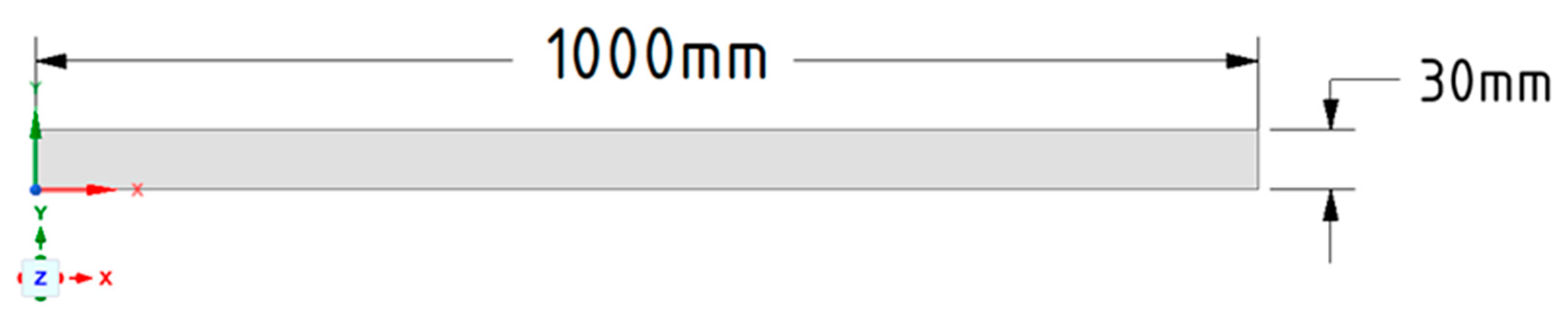
2.2. Mathematical Model in Ansys

The mathematical model consists of a two-dimensional Euler equation that describes the wave propagation velocity, contact discontinuity, and shock discontinuity. The shock tube problem has an analytical solution for the time before the impact of the shock wave on the edge of the tube (Jr. Anderson, J.D. 1989, [35]). The analytical solution to this problem Sod is often used as an example for compressible solvers. An analytical solution of this problem can also be obtained using exact Riemann solvers [36,37]. This paper demonstrates a two-dimensional numerical simulation of the Sod problem in the Ansys Fluent software package.

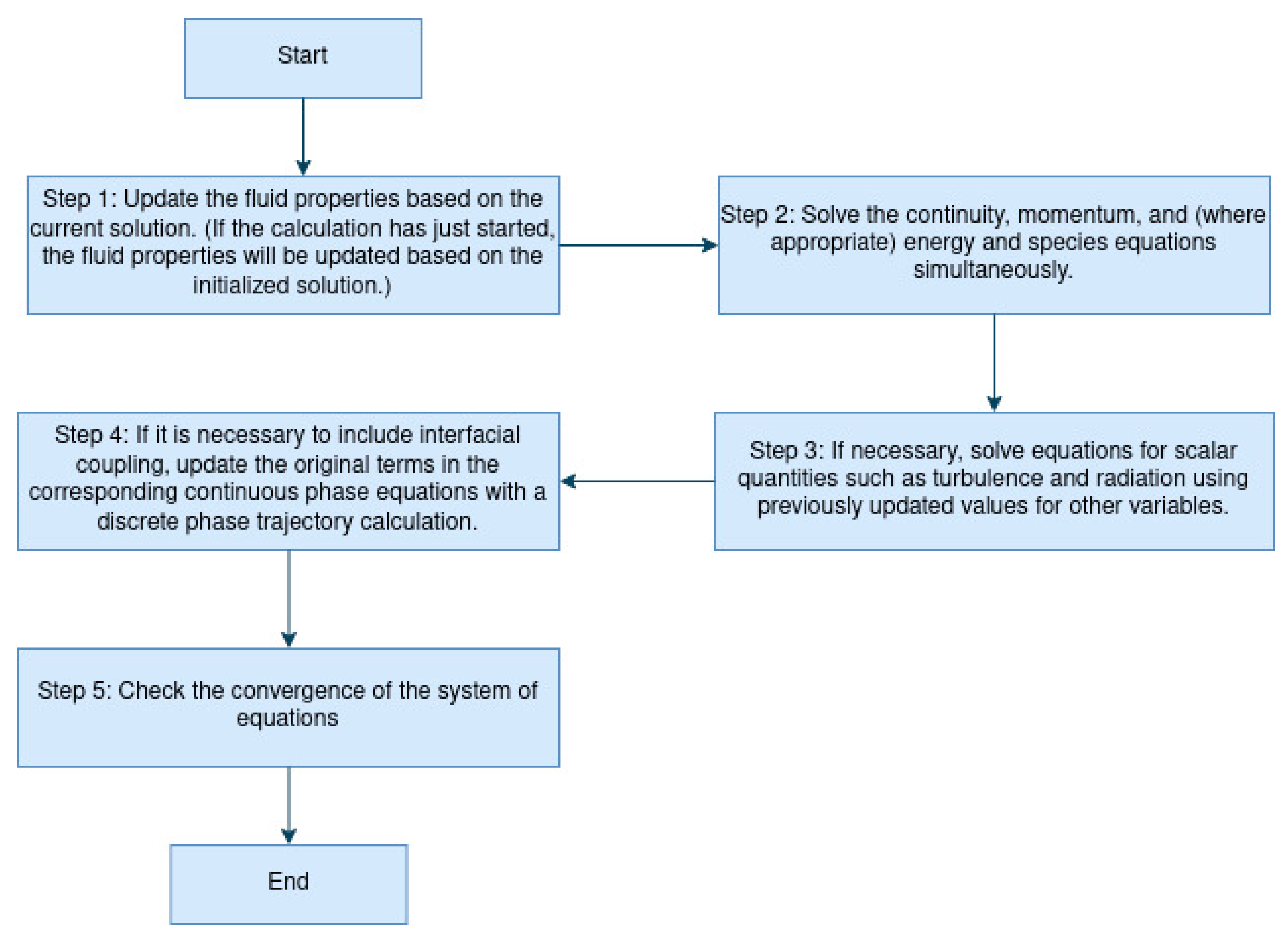
2.3. Numerical Simulation Algorithm in Ansys

The density-based algorithm solves the basic equations of continuity, momentum, and (where appropriate) energy and matter transport simultaneously. The governing equations for additional scalars will be solved subsequently and sequentially (i.e., separately from each other and from the associated set). Since the governing equations are non-linear (and coupled), several iterations of the solve loop must be performed before a convergent solution is obtained. Each iteration consists of the steps described below in Figure 3.

These steps continue until the convergence criteria are met. In the density-based solution method, it is possible to solve a coupled system of equations (continuity, momentum, energy, and species equations, if available) using either the coupled explicit formulation or the coupled implicit formulation. The main difference between explicit and implicit density-based formulations is:

In density-based solution methods, discrete non-linear master equations are linearized to obtain a system of equations for the dependent variables in each computational cell. The resulting linear system is then solved to obtain an updated flow field solution. The method of linearizing the governing equations may take an “implicit” or “explicit” form with respect to the dependent variable (or set of variables) of interest. Implicit or explicit means the following:

-

Implicit: For a given variable, the unknown value in each cell is calculated using a ratio that includes both existing and unknown values from adjacent cells. Therefore, each unknown will appear in more than one equation of the system, and these equations must be solved simultaneously in order to obtain unknown quantities.

-

Explicit: For a given variable, the unknown value in each cell is calculated using a relation that includes only existing values. Therefore, each unknown will only appear in one equation in the system, and the equations for the unknown value in each cell can be solved one at a time to get the unknowns.

In the density-based solution method, there is a choice of using implicit or explicit linearization of the governing equations. This selection only applies to the associated set of master equations. The transport equations for additional scalars are solved separately from the associated set (e.g., turbulence, radiation, etc.). The transport equations are linearized and solved implicitly. Regardless of the choice of implicit or explicit methods, the decision procedure described above is carried out.

If the explicit variant of the density solver is chosen, each equation in the associated set of master equations is linearized explicitly. This will result in a system of equations with N equations for each cell in the domain, and similarly, all dependent variables in the set will be updated at the same time. However, this system of equations is explicit with respect to unknown dependent variables. For example, the x–momentum equation is written such that the updated speed x is a function of the existing values of the field variables. Because of this, a linear equation solver is not needed. Instead, the solution is updated using a multi-stage (Runge–Kutta) solver. There is an additional option to use a multi-grid full approximation storage scheme (FAS) to speed up a multi-stage solver. Thus, the explicit density-based approach solves for all variables $\left(\mathit{p},\mathit{u},\mathit{v},\mathit{w},\mathit{T}\right)$ one cell at a time.

3. Results

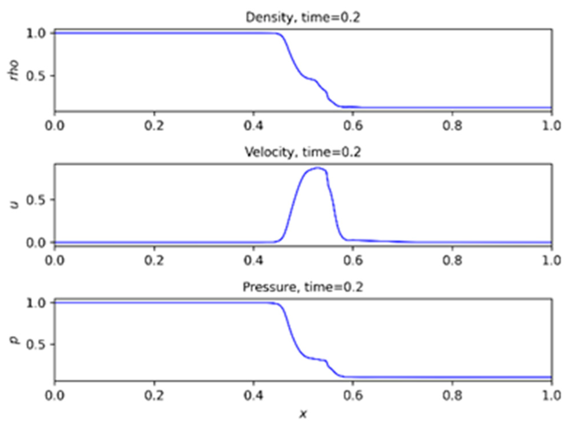
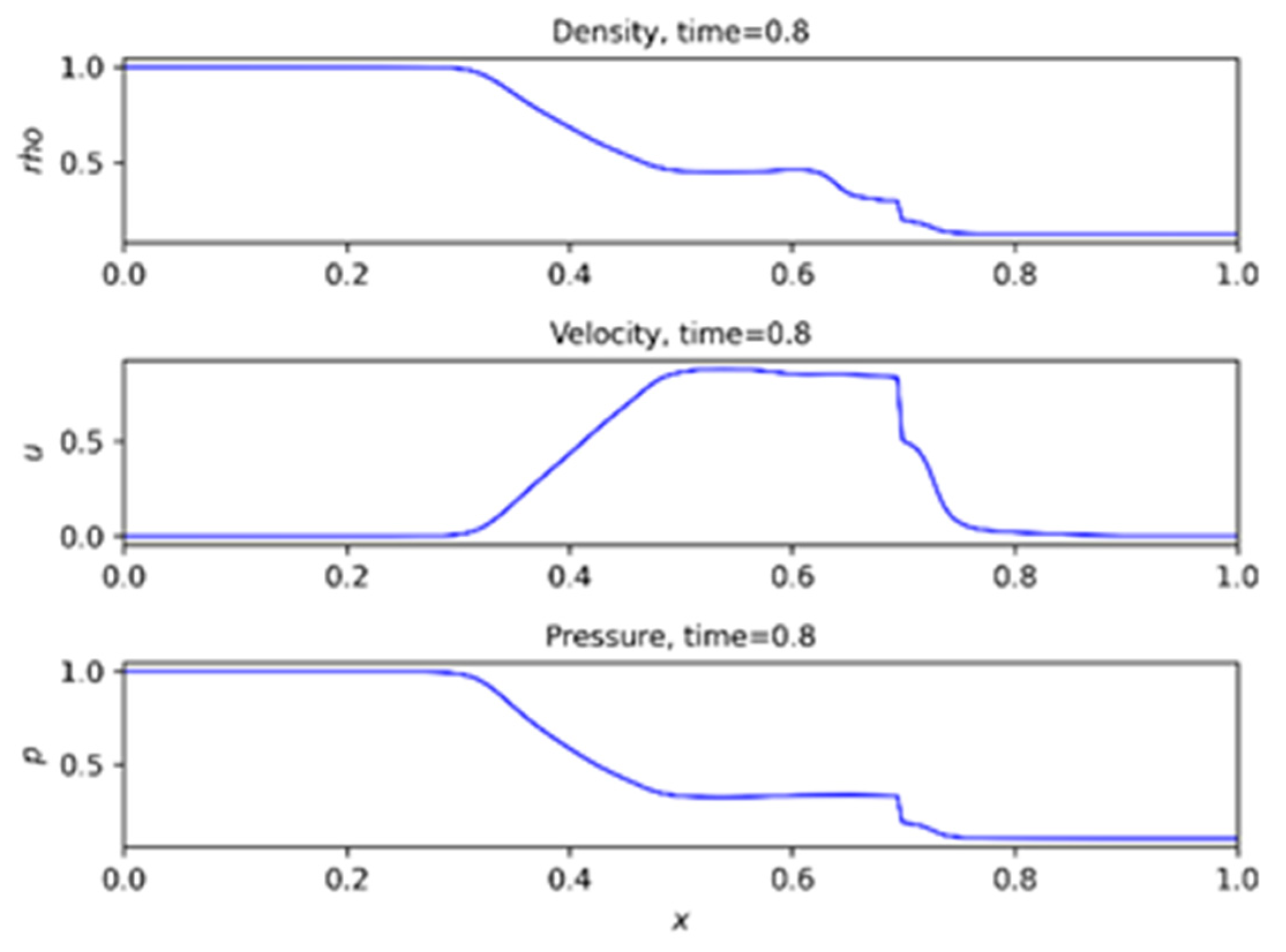
3.1. Numerical Result from PINN

The problem of hydrodynamics with a shock tube is a standard hydrodynamic test problem. The problem is used as a test problem to test the ability of numerical methods to capture characteristics unique to solving conservation laws. The solution for each physical quantity gives a contact discontinuity and a shock wave. The numerical calculation of the shock wave and the contact discontinuity is difficult because the numerical scheme creates artificial dispersion or scattering near the discontinuity points.

To explain the predictive versatility of physics-informed neural network (PINN) modeling, the case of the Euler problem was selected for analysis in this research. For a general universal PINN model, it is proposed to analyze several different cases representing diverse conditions and carefully justify the choice and representativeness of each of them. The PINN model presented can predict the clogging relationships in different scenes accurately.

In our study, we considered the following architecture of PINN. The input to this architecture is two vectors of values t and tix, and the result is three vectors of values u, p, and ρ (velocity, pressure, and density). The main hyperparameters of PINN are presented in

Table 1. The main hyperparameters of PINN architecture.

Parameters	PINN
Number of layers	6
Activation function	Tanh
Optimizer	Adam
Number of epochs	7500
Learning rate	0.001
Loss function	MSE

. The hyperparameter of the neural network is four hidden layers with 30 neurons in each layer, and the optimizing procedure is the Adam optimizer with a learning rate of 0.001. For each layer, the function of activation is the tanh function. The loss function is the MSE for the given data and initial condition, as presented in Equations (4) and (5).

Figure 4, Figure 5 and Figure 6 show the prediction results using PINN for density, pressure, and velocity over time = 0.2, 0.6, 0.8, respectively. In these figures, we can notice that when the shock moved, the density changed from x = 0.5 and t = 0.2 to x = 0.7 and t = 0.8. It showed that the consistency of fluid was changing, i.e., the flow became saturated with rock particles; in our case, we observed that sedimentation occurred. The shock wave has a smooth trend, although it should be a sharp feature. In this paper, we will compare the PINN solution with the Ansys solution.

The use of the PINN approach opens up possibilities for solving a general class of discontinuous solutions of compressible Euler equations. This is achieved due to the ability to capture physical phenomena such as impacts, contact breaks, and rarefaction.

In Figure 5, Figure 6 and Figure 7, the velocity behavior shows scattering near the impact angles. This allows for computational errors, and one of the goals of PINN is to find solutions that are as accurate as possible.

3.2. Numerical Result from ANSYS

This study aims to model the problem of the Sod shock tube. The task is to simulate the propagation of a normal shock wave inside a shock tube under experimental conditions. The obtained numerical results are compared with the results obtained using the PINN method, which is a widely popular method in fluid flow simulation.

To check the correctness and accuracy of the mathematical model used, the test problem was solved numerically, based on the research of other authors.

For this, a 2D shock tube model was used, which is a long metal tube consisting of two chambers and separated by a diaphragm. The diaphragm separates the high-pressure area from the low-pressure area. After the diaphragm is removed, the shock wave and the contact discontinuity begin to move to the region of initially low pressure, and the rarefaction wave moves to the region of initially high pressure (Khodadadi Azadboni et al., 2013, [38]). Two different solvers were used in the problem: driver and driven. The chamber used consists of two gases with a high-pressure ratio. Thus, one chamber is filled with high-pressure ideal gas, the driver, and the other chamber, vice versa, is low-pressure, and is called the driven. A schematic representation of the studied reservoir is shown in Figure 7. The length of this reservoir is L_b = 1 m and H_b = 0.03 m. When modeling, a piercing mechanism was built into the diaphragm, which breaks the diaphragm under given conditions. When the contact is suddenly broken, a series of pressure waves are created that cause a shock wave.

The computational grid plays a fundamental role in ensuring accuracy and detail when conducting calculations using the PINN and Ansys methods. It enables more precise and detailed modeling of physical phenomena, ultimately leading to more reliable results and a deeper understanding of the processes under study.

Therefore, for this task, a structured computational mesh was used, the total number of elements of which was 30,000, and the number of nodes was 31,031. Face meshing = 1 × 10⁻³ m. The total duration of the task calculation is 3000 time steps. The initial conditions for the test problem for Ansys are presented in Figure 8.

The obtained numerical results were compared with the results obtained by using the PINN method. As can be seen, the numerical simulation results show exact solutions to the problem with a clear shock effect. In solving the problem using PINN, the shock effect is not explicitly shown.

The obtained numerical results were compared with the results obtained using the PINN method at different time intervals, and these results were compared. As can be seen, numerical modeling provides accurate solutions to this problem, displaying the clear effect of shock waves. When solving the same problem using the PINN method, the shock wave effect is not explicitly highlighted.

This difference in results can be explained by the fact that the PINN method employs artificial neural networks to solve physical problems. In this method, neural networks are trained to integrate physical laws and conditions into the solution process. Thus, the PINN method strives to create smooth and continuous solutions, which may not clearly represent explicit physical effects, such as shock waves, in the results.

In numerical modeling, on the other hand, problems are solved using numerical methods that can more accurately capture physical phenomena, such as shock waves. These methods discretize the space into a grid and solve equations on each grid element, allowing for a more detailed description of physical processes.

Therefore, comparing numerical results with the results obtained using the PINN method allows for the identification of differences in approaches and the advantages of each method. The former provides smoother solutions and reduces the computational complexity but may not highlight some physical effects, while the latter allows for more accurate modeling of physical processes but may require higher computational resources. Figure 9 shows comparisons of PINN solutions with exact solutions from Ansys at various x locations.

We can observe that while we can achieve accurate results for density, our ability to make precise predictions for velocity and pressure is limited. This limitation arises from the fact that the flow has not yet reached the area between the shock and the right boundary. Thus, attempting to incorporate pressure information from this region into the avail-able data and equations would not uncover the actual pressure and velocity fields within the desired domain.

As the results show, numerical simulation more clearly shows the shock effect, where the boundaries of pressure, velocity, and density changes are. And the obtained results of the PINN method are smoother, since using a neural network, training was carried out considering the physical constraints and conditions of the problem. However, the calculation time (including training time) using the PINN method is much less than when using numerical simulation.

The analysis of the conducted research leads to the conclusion that comparing the results obtained using numerical modeling and the PINN method is significant for solving problems related to river dynamics and pollution processes. Both methods have their strengths and are applicable depending on the objectives and characteristics of the task.

Numerical modeling provides precise solutions and allows for capturing explicit physical effects, such as shock waves. This is achieved via the careful discretization of space into a grid and the numerical solution of the equations on each grid element. This approach is better suited to tasks where it is necessary to describe physical processes and effects in detail.

On the other hand, the PINN method offers smoother and more continuous solutions, as neural networks are trained to integrate physical laws and conditions. This method reduces the computational complexity and can be effective in cases where obtaining fast results is crucial and when explicit physical effects are not the primary concern.

Therefore, the choice between numerical modeling and the PINN method depends on the specific objectives and requirements of the task. The former allows for a more precise description of physical phenomena but may require substantial computational resources. The latter provides smoother solutions and faster computations over a short period but may not highlight certain physical effects.

Comparing results, as shown in Figure 9, can assist researchers and engineers in selecting the approach most suitable for their specific task. This enables the attainment of more reliable and efficient solutions when modeling river dynamics and water pollution processes.

4. Discussion

PINN could be used for the prediction of fluid flow in several different contexts such as water supply, oil wells, etc. Moreover, the ability to adapt to different conditions and changing parameters makes it possible to tune and learn from different datasets and changes for each new scenario. Due to the versatility of the PINN model, it can be applied in various cases, and the results confirm its high accuracy and reliability in different application areas.

In this discussion, we presented a comparative analysis of the physics-informed neural network method and classical numerical simulation techniques for solving problems related to the simulation of physical processes. Both approaches have their advantages and limitations, and understanding their differences is crucial in selecting the most suitable method for a given problem.

In contrast, classical numerical simulation relies on solving differential equations that describe physical processes through numerical integration methods. This approach has a well-established foundation in scientific computing and is widely used in various fields. Numerical simulations are highly accurate when appropriate numerical methods and parameters are employed. However, they can be computationally intensive, especially for complex problems or high-resolution simulations.

Table 2. Time comparison of the PINN method and numerical simulation.

	Time (s)	Element Numbers or Parameters
PINN	1948	4833
Ansys	1080	50,300
	780	30,000
	240	4800

provides a comparative analysis of the time performance of the PINN method and numerical simulation, measured in seconds and the number of elements or parameters involved. The results demonstrate that the PINN method requires 1948 s with 4833 parameters of neural networks (weights and biases), while Ansys simulation takes 1080 s with 50,300 elements, 780 s with 30,000 elements, and 240 s with 4800 elements. It is important to note that the PINN model was trained for 7500 epochs on a CPU resource, matching the computational platform used for Ansys simulation. However, it is important to consider the following factors: (a) the training time of the PINN method may depend on the complexity of the task, the amount of training data, and the resources used for training; (b) the execution time of numerical modeling in Ansys Fluent depends on the grid size, geometry complexity, the chosen numerical methods, and computational resources.

The choice between the PINN method and numerical simulation depends on several factors, including the availability of data, problem complexity, and computational resources. While the PINN method may offer computational advantages, its accuracy may be compromised in cases with insufficient or inaccurate data. Additionally, training the neural network under certain physical conditions can be challenging. On the other hand, numerical simulation excels in terms of accuracy but may require substantial computational resources, making it less efficient for some applications.

We investigated the fact that siltation affects the density of a fluid, and this change can be monitored using various density parameters. In addition, by using flow rate analysis, we can implicitly detect the presence of a blockage. The main contribution of this work is integrating PINN for a more reliable and accurate method of clog identification compared to previous simulation methods.

In conclusion, both the PINN method and numerical simulation play vital roles in simulating physical processes. Researchers and engineers must carefully evaluate the specific requirements and constraints of their problems to determine the most suitable approach. Furthermore, ongoing advancements in computational methods, including the integration of neural networks, continue to expand the possibilities for solving complex physical problems efficiently and accurately.

5. Conclusions

This paper proposes a comparative analysis of the PINN method and numerical simulation for estimating the indicators of velocity, pressure, and density in the aquatic environment. Thanks to the PINN method, numerical results obtained on time can be used for subsequent numerical modeling of the silting of river channels and channels. Predicting the above indicators is important in preventing river pollution due to sedimentation. This method makes it possible to evaluate various fluid types (compressible, incompressible, Newtonian, non-Newtonian, etc.). Also, during the modeling process, accurate numerical results were obtained, demonstrating the behavior of the flow of compressible fluids.

Comparing the results of PINN and numerical simulations in Ansys, the profiles of the velocity, density, and pressure indicators are the same, except for the areas where the shock effect occurs. Also, PINN simulation results can be obtained faster than Ansys numerical simulations, which is a clear advantage. It should be noted that numerical simulation for a natural area requires a lot of computational costs, depending on the area of calculation, since the number of elements in the construction of the grid plays an important role. For this reason, in some calculations used to prevent the pollution of rivers due to sedimentation in a real area, it is better to use the PINN method.

With the PINN method, it is possible to estimate different fluid types, for example, in terms of density, and further model the siltation of river channels for more complex conditions and measurements.

In future work, the PINN method will be extended to higher dimensions, and real problems in river silting will be modeled. In future works, the Euler and Navier–Stokes equations solved using the PINN method will be investigated, and we will also consider a comparative analysis of the PINN and FEM methods.

References

1. Zhang, Z.; Lu, M.; Ji, S.; Yu, H.; Nie, C. Rich CNN Features for Water-Body Segmentation from Very High Resolution Aerial and Satellite Imagery. Remote Sens. 2021, 13, 1912. [Google Scholar] [CrossRef]
2. Hasan, O.; Smrkulj, N.; Miko, S.; Brunović, D.; Ilijanić, N.; Šparica Miko, M. Integrated Reconstruction of Late Quaternary Geomorphology and Sediment Dynamics of Prokljan Lake and Krka River Estuary, Croatia. Remote Sens. 2023, 15, 2588. [Google Scholar] [CrossRef]
3. Wu, X.; Feng, X.; Fu, B.; Yin, S.; He, C. Managing erosion and deposition to stabilize a silt-laden river. Sci. Total Environ. 2023, 881, 163444. [Google Scholar] [CrossRef]
4. Sun, L.; Guo, H.; Wang, H.; Zhang, B.; Feng, H.; Wu, S.; Siddique, K.H.M. Deep learning for check dam area extraction with optical images and digital elevation model: A case study in the hilly and gully regions of the Loess Plateau, China. Earth Surf. Process. Landf. 2023. [Google Scholar] [CrossRef]
5. Best, J.; Darby, S.E. The Pace of Human-Induced Change in Large Rivers: Stresses, Resilience, and Vulnerability to Extreme Events. One Earth 2020, 2, 510–514. [Google Scholar] [CrossRef] [PubMed]
6. Marren, P.M.; Grove, J.R.; Webb, J.A.; Stewardson, M.J. The Potential for Dams to Impact Lowland Meandering River Floodplain Geomorphology. Sci. World J. 2014, 2014, 1–24. [Google Scholar] [CrossRef] [PubMed]
7. Hawley, R.J. Making Stream Restoration More Sustainable: A Geomorphically, Ecologically, and Socioeconomically Principled Approach to Bridge the Practice with the Science. BioScience 2018, 68, 517–528. [Google Scholar] [CrossRef] [PubMed]
8. Merembayev, T.; Mukhamediev, R.; Amirgaliyev, Y.; Malakhov, D.; Terekhov, A.; Kuchin, Y.; Yakunin, K.; Symagulov, A. The Application of Machine Learning Technique to Soil Salinity Mapping in South of Kazakhstan. In Proceedings of the 15th Asian Conference on Intelligent Information and Database Systems, Phuket, Thailand, 24–26 July 2023; pp. 244–253. [Google Scholar]
9. Constantine, J.A.; Dunne, T.; Ahmed, J.; Legleiter, C.; Lazarus, E.D. Sediment supply as a driver of river meandering and floodplain evolution in the Amazon Basin. Nat. Geosci. 2014, 7, 899–903. [Google Scholar] [CrossRef]
10. Dottori, F.; Szewczyk, W.; Ciscar, J.-C.; Zhao, F.; Alfieri, L.; Hirabayashi, Y.; Feyen, L. Increased human and economic losses from river flooding with anthropogenic warming. Nat. Clim. Change 2018, 8, 781–786. [Google Scholar] [CrossRef]
11. Sinha, R.; Gupta, A.; Mishra, K.; Tripathi, S.; Nepal, S.; Wahid, S.M.; Swarnkar, S. Basin-scale hydrology and sediment dynamics of the Kosi River in the Himalayan foreland. J. Hydrol. 2019, 570, 156–166. [Google Scholar] [CrossRef]
12. Phillips, C.B.; Masteller, C.C.; Slater, L.J.; Dunne, K.B.J.; Francalanci, S.; Lanzoni, S.; Merritts, D.J.; Lajeunesse, E.; Jerolmack, D.J. Threshold constraints on the size, shape and stability of alluvial rivers. Nat. Rev. Earth Environ. 2022, 3, 406–419. [Google Scholar] [CrossRef]
13. Powledge, G.R.; Ralston, D.C.; Miller, P.; Chen, Y.H.; Clopper, P.E.; Temple, D.M. Mechanics of overflow erosion on embankments. I: Research activities; II/hydraulic and design considerations. J. Hydraul. Eng. 1989, 115, 1040–1075. [Google Scholar] [CrossRef]
14. Schmocker, L.; Hager, W.H. Modelling dike breaching due to overtopping. J. Hydraul. Res. 2009, 47, 585–597. [Google Scholar] [CrossRef]
15. Froehlich, D.C. Embankment dam breach parameters and their uncertainties. J. Hydraul. Eng. 2008, 134, 1708–1721. [Google Scholar] [CrossRef]
16. Fetzer, J.; Holzner, M.; Plötze, M.; Furrer, G. Clogging of an Alpine streambed by silt-sized particles—Insights from laboratory and field experiments. Water Res. 2017, 126, 60–69. [Google Scholar] [CrossRef]
17. Yao, P.; Su, M.; Wang, Z.; van Rijn, L.C.; Zhang, C.; Chen, Y.; Stive, M.J.F. Experiment inspired numerical modeling of sediment concentration over sand–silt mixtures. Coast. Eng. 2015, 105, 75–89. [Google Scholar] [CrossRef]
18. Kazidenov, D.; Khamitov, F.; Amanbek, Y. Coarse-graining of CFD-DEM for simulation of sand production in the modified cohesive contact model. Gas Sci. Eng. 2023, 113, 204976. [Google Scholar] [CrossRef]
19. Merembayev, T.; Amanbek, Y. Natural Fracture Network Model Using Machine Learning Approach. In Proceedings of the 24th International Conference on Computational Science and Its Applications, Athens, Greece, 3–6 July 2023; pp. 384–397. [Google Scholar]
20. Ecemis, N. Experimental and numerical modeling on the liquefaction potential and ground settlement of silt-interlayered stratified sands. Soil Dyn. Earthq. Eng. 2021, 144, 106691. [Google Scholar] [CrossRef]
21. Narbayev, B.; Amanbek, Y. Finite Element Model for Wind Comfort Around a Tall Building: A Case Study of Tower of Qazaqstan. In Proceedings of the Computational Science and Its Applications—ICCSA 2022 Workshops, Malaga, Spain, 4–7 July 2022; pp. 540–553. [Google Scholar]
22. Omarova, P.; Merembayev, T.; Amirgaliyev, Y. Mathematical modeling of water movement during a dam break using the vof method. Sci. J. Astana IT Univ. 2023, 14, 104–115. [Google Scholar] [CrossRef]
23. Soares-Frazão, S.; Le Grelle, N.; Spinewine, B.; Zech, Y. Dam-break induced morphological changes in a channel with uniform sediments: Measurements by a laser-sheet imaging technique. J. Hydraul. Res. 2007, 45 (Suppl. S1), 87–95. [Google Scholar] [CrossRef]
24. Goutiere, L.; Soares-Frazão, S.; Zech, Y. Dam-break flow on mobile bed in abruptly widening channel: Experimental data. J. Hydraul. Res. 2011, 49, 367–371. [Google Scholar] [CrossRef]
25. Buribayev, Z.; Merembayev, T.; Amirgaliyev, Y.; Miyachi, T. The Optimized Distance Calculation Method with Stereo Camera for an Autonomous Tomato Harvesting. In Proceedings of the 2021 IEEE International Conference on Smart Information Systems and Technologies (SIST), Nur-Sultan, Kazakhstan, 28–30 April 2021; pp. 1–5. [Google Scholar]
26. Kenshimov, C.; Mukhanov, S.; Merembayev, T.; Yedilkhan, D. A Comparison of Convolutional Neural Networks for Kazakh Sign Language Recognition. East. Eur. J. Enterp. Technol. 2021, 113, 44–54. [Google Scholar] [CrossRef]
27. Yeleussinov, A.; Amirgaliyev, Y.; Cherikbayeva, L. Improving OCR Accuracy for Kazakh Handwriting Recognition Using GAN Models. Appl. Sci. 2023, 13, 5677. [Google Scholar] [CrossRef]
28. Sukumar, N.; Srivastava, A. Exact imposition of boundary conditions with distance functions in physics-informed deep neural networks. Comput. Methods Appl. Mech. Eng. 2022, 389, 114333. [Google Scholar] [CrossRef]
29. ANSYS-FLUENT, version 12.0; Theory Guide; Ansys: Canonsburg, PA, USA, April 2009.
30. Meng, X.; Li, Z.; Zhang, D.; Karniadakis, G.E. PPINN: Parareal physics-informed neural network for time-dependent PDEs. Comput. Methods Appl. Mech. Eng. 2020, 370, 113250. [Google Scholar] [CrossRef]
31. Cheng, C.; Meng, H.; Li, Y.-Z.; Zhang, G.-T. Deep learning based on PINN for solving 2 DOF vortex induced vibration of cylinder. Ocean. Eng. 2021, 240, 109932. [Google Scholar] [CrossRef]
32. Huang, Y.H.; Xu, Z.; Qian, C.; Liu, L. Solving free-surface problems for non-shallow water using boundary and initial conditions-free physics-informed neural network (bif-PINN). J. Comput. Phys. 2023, 479, 112003. [Google Scholar] [CrossRef]
33. Holland, P. Hydrodynamics, Particle Relabelling and Relativity. Int. J. Theor. Phys. 2011, 51, 667–683. [Google Scholar] [CrossRef]
34. Alemi Ardakani, H.; Bridges, T.J. Dynamic coupling between shallow-water sloshing and horizontal vehicle motion. Eur. J. Appl. Math. 2010, 21, 479–517. [Google Scholar] [CrossRef]
35. Anderson, J.D., Jr. Modern Compressible Flow with Historical Perspective, 2nd ed.; McGraw Hill Professional Publishing: New York, NY, USA, 1989. [Google Scholar]
36. Anderson, J.D., Jr. Modern Compressible Flow: With Historical Perspective, 3rd ed.; McGraw-Hill: New York, NY, USA, 2003. [Google Scholar]
37. Torro, E.F. Riemann Solvers and Numerical Methods for Fluid Dynamics: A Practical Introduction, 3rd ed.; Springer: Cham, Switzerland, 1997. [Google Scholar]
38. Khodadadi, A.R.; Malekbala, M.R.; Khodadadi, A.F. Evaluate Shock Capturing Capability with the numerical method in OpenFOAM. J. Therm. Sci. 2013, 17, 1255–1260. [Google Scholar] [CrossRef]
Figure 1. Concept implementation scheme PINN.
Applsci 13 11983 g001
Figure 2. An example of domain extension in the Sod inverse problem in Section IV.C. This domain [0; 1] extended to [−2.625; 2.5].
Applsci 13 11983 g002
Figure 3. The flowchart of simulation in Ansys.
Applsci 13 11983 g003
Figure 4. Solving the problem using PINN for a period of time = 0.2.
Applsci 13 11983 g004
Figure 5. Solving the problem using PINN for a period of time = 0.6.
Applsci 13 11983 g005
Figure 6. Solving the problem using PINN for a period of time = 0.8.
Applsci 13 11983 g006
Figure 7. Geometry of the test problem.
Applsci 13 11983 g007
Figure 8. Initial conditions for the test problem.
Applsci 13 11983 g008
Figure 9. A comparison of density, pressure, and velocity with the exact solutions. (a) Density. (b) Pressure. (c) Velocity.
Applsci 13 11983 g009