Abstract
Quality control procedures in the manufacturing of tableware ceramics require a demanding, monotonous, subjective, and faulty human manual inspection. This paper presents two machine learning strategies and the results of a semi-automated visual inspection of ceramics tableware applied to a private dataset acquired during the VAICeramics project. In one method, an anomaly detection step was integrated to pre-select possible defective patches before passing through an object detector and defects classifier. In the alternative one, all patches are directly provided to the object detector and then go through the classification phase. Contrary to expectations, the inclusion of the anomaly detector demonstrated a slight reduction in the performance of the pipeline, which may result from error propagation. Regarding the proposed methodology for defect detection, it exhibits average performance in monochromatic images with more than 600 real defects in total, efficiently identifying the most common defect classes in highly reflective surfaces. However, when applied to newly acquired images, the pipeline encounters challenges revealing a lack of generalization ability and experiencing limitations in detecting specific defect classes, due to their appearance and limited available samples used for training. Only two defect types presented high classification performance, namely Dots and Cracked defects.
1. Introduction
The industry of ceramics is an ancient and highly competitive sector with an extreme financial impact for many countries, particularly reflected in terms of exports. Ensuring the quality of ceramic products, such as tableware pieces, is of supreme importance, as even minor defects can impact both their aesthetics and structural integrity. Unexpected additional costs for the manufacturing company can arise from contract penalties, selling price reductions, whole batch returns, unnecessary usage of the oven in false positive cases, and extraordinary hours paid to factory workers for re-inspection. Nevertheless, quality control within this industry essentially relies on human visual inspection performed by trained operators, which requires a substantial allocation of human resources and is inherently time-consuming and prone to error. The complexity is even increased by variable glazing, shapes, dimensions, and colors. Consequently, the demand for advanced and efficient quality control approaches has given rise to the development of computer-aided visual inspection systems.
In this study, we introduce a comprehensive methodology for multi-class defect detection in tableware ceramics, presenting a semi-automated process designed on the shop floor. Therefore, this work aims to:
- Develop an end-to-end system capable of efficiently identifying multiple classes of defects in challenging objects;
- Investigate the impact of incorporating an anomaly detection step to pre-select possible defective image patches;
- Conduct semantic segmentation to differentiate regions of the ceramic pieces, as the defect’s location influences the manufacture quality of each piece (to set market value).
- Promote innovation within the ceramics manufacturing sector and contribute to product quality assurance, using the variable dimensions, colors, and shapes of pieces and defects.
The remainder of the manuscript is organized as follows: Section 2 presents state-of-the-art approaches for defect and anomaly detection; Section 3 details the dataset employed in this work and the data acquisition process, and presents the methodology adopted for each module of the proposed pipeline; Section 4 reports the results obtained for the components and compares the incorporation of anomaly detection in the pipeline; Section 5 presents conclusions and possible modifications in future work.
2. Related Work
The application area of table ceramics has very specific requirements as highly reflective surfaces along the piece, several zones to inspect with distinct morphology and texture background, and complex defects make the development of automatic inspection solutions far from trivial. The existing commercial solutions for automatic visual inspections in related application areas are generally very specific to certain types of ceramic (raw material), types of pieces (geometry) and types of defects. This is the case of OPTO machines’ solutions [1], with product size and shape limitations, and SCIOTEX [2], which has limited defect typology. These are solutions tailored to the needs of their existing customers, and are not so widespread in the tableware ceramics industry. RSIP Vision [3] employs machine learning algorithms for geometric defects, but inspections are applied before mass production (without reflective glaze) and are not suitable for tableware pieces. The SYSTEM CERAMICS [4] and SACMI [5] technologies are aimed at the floor and wall ceramics sub-sector, where the pieces are typically flat (tiles, slabs, etc.) and are, therefore, not very comparable to the solution proposed in this work.
To the best of our knowledge, there are no public datasets available on tableware ceramic pieces, which motivated the research team to propose a dedicated setup for image acquisition. However, some databases in further applications have been used for tackling related challenges such as small-size defects in high-resolution images, or for dealing with highly reflective surfaces. KolektorSDD [6] includes defects in electrical commutator with microscopic fractions or cracks, but images are too noisy compared our application problem. The NEU Surface Defect Database [7] is focused on hot-rolled steel strip surface defects, with low resolution and only one type of defect per image. The Severstal [8] steel defect dataset has four classes of defects with some diversity in size in steel manufacturing. This dataset inspired some preliminary work of our research team, who tested the implementation of the DeepLabV3+ architecture for semantic segmentation that would be promising for one of the modules (Piece Zone presented in Section 3.3) of the main proposed pipeline.
Tao et al. [6] designed a cascaded autoencoder (CASAE) for the segmentation and classification of metallic defects. The cascading network transforms the input defect image into a pixel-wise prediction mask based on semantic segmentation. The defect regions of segmented results are classified into their specific classes via a compact convolutional neural network (CNN). Tabernik et al. [9] presented a segmentation-based deep-learning architecture designed for the detection and segmentation of surface anomalies and is demonstrated on a specific domain of surface-crack detection in industrial electronics. The first stage implements a segmentation network that performs a pixel-wise localization of the surface defect. Training this network with a pixel-wise loss effectively considers each pixel as an individual training sample, thus increasing the effective number of training samples and preventing overfitting. The second stage, where binary-image classification is performed, includes an additional network that is built on top of the segmentation network and uses both the segmentation output as well as features of the segmentation net.
In recent years, anomaly detection techniques have gained significant interest in the field of defect detection. These techniques leverage machine learning algorithms to automatically identify deviations from normal patterns in images. Due to their ability to carry out distribution fitting, Generative Adversarial Networks (GANs) have been used to this end, assuming that by learning feature representations of normal samples in the latent space, anomalous samples may be identified [10]. Taking this into account, some works were already developed, aiming to detect defects in several industrial applications. Liu et al. [11] used a GAN-based approach for detecting surface defects of strip steel. In the work of Lai et al. [12], a framework for anomaly detection in industrial datasets (a wood texture and a solar panel datasets) was proposed, which also relies on a generative network. Another semi-supervised approach was presented in [13], intending to classify steel surface defects by using a combination of a Convolutional Autoencoder (CAE) and Semi-supervised Generative Adversarial Networks (SGAN). GAN-based anomaly detection methods have also been explored in other application fields, such as medical diagnosis, infrastructure inspection, or even other detection tasks, such as network security or finance fraud [10]. Regarding medical diagnosis, for instance, Schlegl et al. [14] proposed fast AnoGAN (f-AnoGAN), an improved version of AnoGAN [15], which intends to identify anomalous samples and segments in patches of clinical optical coherence tomography (OCT) scan images.
As far as we know, none of the commercial solutions and scientific methods for visual inspection of defects in the tableware ceramics domain, include piece zone detection to correctly assign the market value of the piece, anomaly detection for selecting defect candidates, nor have been evaluated using tableware pieces with variable dimensions, colors, and shapes.
3. Materials and Methods
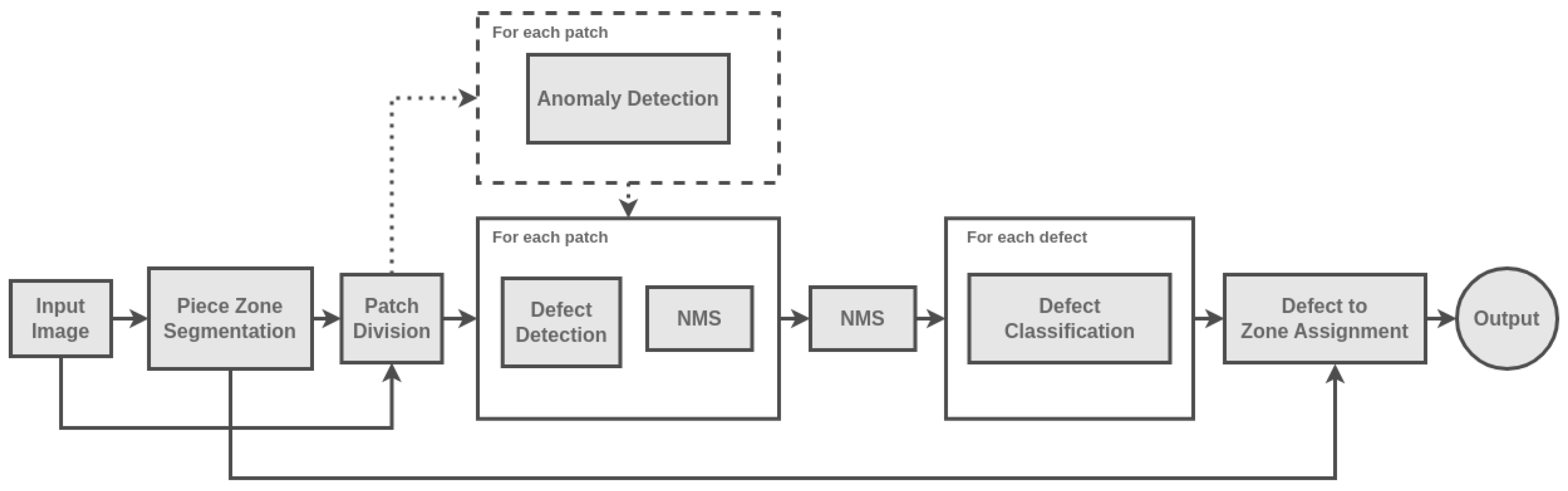
Throughout this work, four machine learning modules were developed, aiming to assist the inspection of defects in ceramics tableware. These modules comprised a piece zone segmentor to identify the relevant regions of the ceramics pieces (Section 3.3), an anomaly detection module to select possible defective pieces (Section 3.4), a defect detector to detect defects in ceramic pieces (Section 3.5) and, finally, a classification module to categorize different types of defects (Section 3.6). Each module was first developed and evaluated independently, before being aggregated in a semi-automated pipeline (Figure 1) that is able to visually inspect ceramics tableware through the identification and characterization of defects.
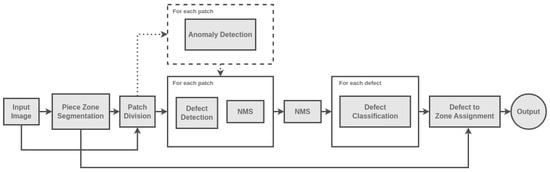
Figure 1.
Overview of the pipeline developed in this work towards the automated visual inspection of tableware ceramics.
The initial step of the pipeline, Piece Zone Segmentation, involves the separation of distinct zones within the ceramic plates. Considering this information, the input image is cropped to include solely the plate area and it is then divided into patches of dimensions of , with a 50% overlap between adjacent patches.
Following the segmentation step, the pipeline offers an optional module, Anomaly Detection. This module analyzes each patch individually to determine the presence of any defects. Patches that are identified as containing defects are then passed on to the Defect Detection model, which generates bounding box predictions encompassing the defect areas. To refine the predictions, the pipeline applies a two-step process. First, a Non-Maximum Suppression (NMS) algorithm selects the most suitable bounding box among a collection of overlapping boxes within each patch, considering only predictions with confidence score higher than 90%. Subsequently, the coordinates of the selected boxes are transformed back to the original image coordinate space, followed by a second NMS operation to filter out redundant detections resulting from overlapping bounding boxes.
The final component of the pipeline is the Defect Classification model, responsible for identifying the specific type of defect present. This classification is subsequently associated with the corresponding zone in which the defect occurs, leading to the final decision regarding the defect analysis.
3.1. Experimental Setup
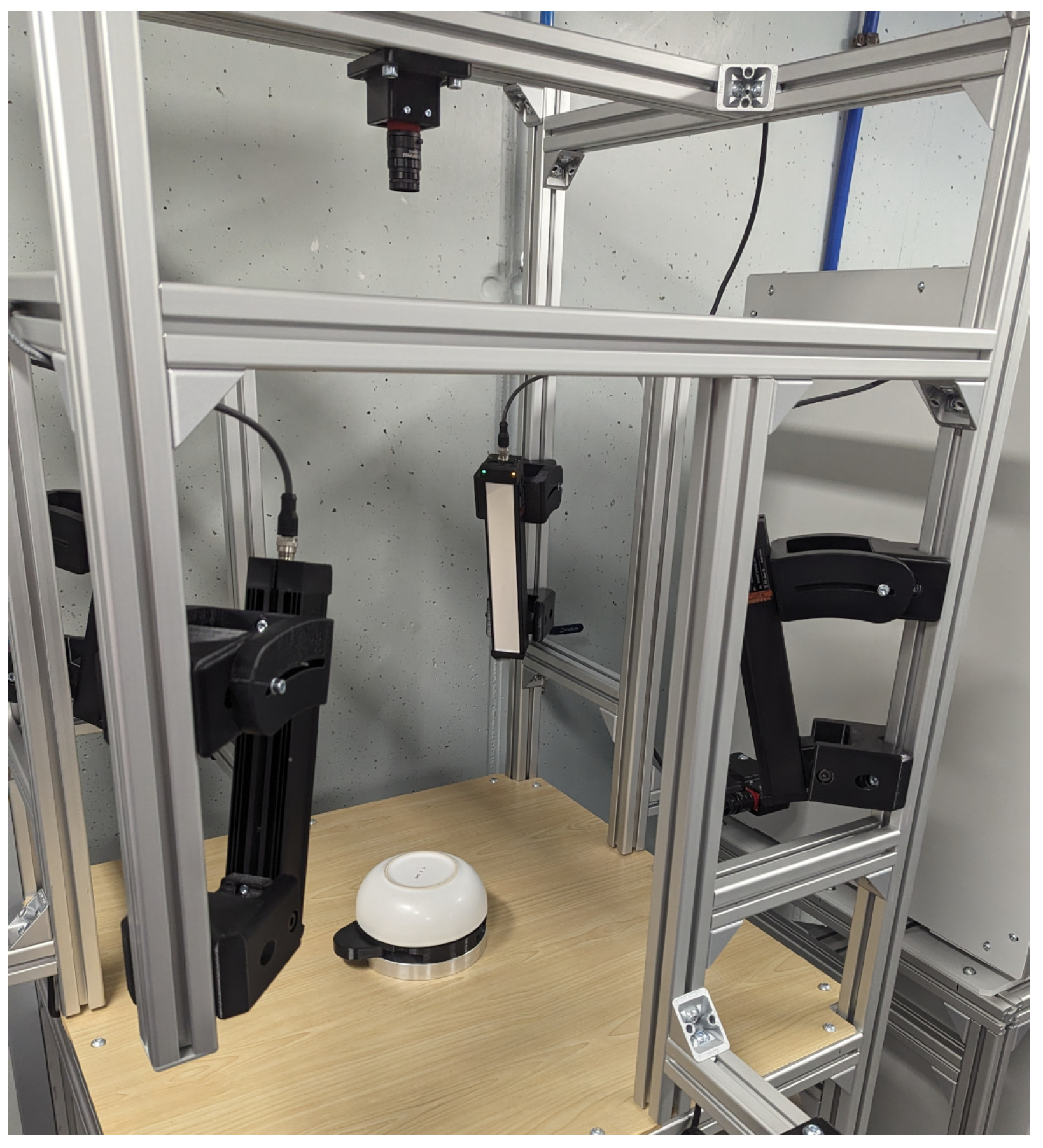
The image acquisition setup was composed of a smart edge device with a GPU (NVIDIA Jetson AGX Xavier), four infrared light bars (TPL Vision BLBAR-250-850), and a 12 megapixel monochromatic industrial camera (Allied Vision Alvium 1800 u-1240m) with lens and polarizer, as represented in Figure 2. The proposed setup was able to achieve 10 pixels per mm. The smart edge device was responsible for controlling the acquisition equipment and all inference processing, being the corresponding computing times presented in Section 4.5.

Figure 2.
Experimental setup developed for image acquisition.
3.2. Data Acquisition
Table 1 provides a comprehensive overview of the frequency of defect classes observed in each batch of image acquisitions. Moreover, the number of ceramic plates examined in each batch is also highlighted.

Table 1.
Dataset description.
Batches 1, 2, 3, and 4 were specifically utilized for training and validation in this study for the development of the models, comprising the first set of images (set 1). Batches 5 and 6 were acquired later and reserved for testing purposes, forming the second set of images (set 2). Visual representations of each defect class are presented in Figure 3. An analysis of the defect class distribution highlights notable variations. Defects such as Defect-10 and Defect-12 exhibit a higher occurrence rate, observed across multiple batches. In contrast, Defects 2 and 13 have a minimal presence within the dataset. Defects 14 and 15 exclusively appear in plates from the last two batches, indicating a more recent occurrence. The observed distribution indicates a significant class imbalance among the defect categories, with certain classes being more prevalent, while others are relatively rare.
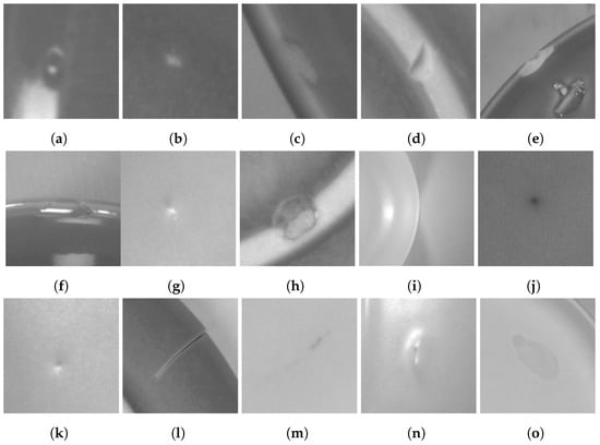
Figure 3.
Examples for each defect class, with variable shapes and dimensions. (a) Defect-1: Blister; (b) Defect-2: Glaze roll; (c) Defect-3: Lack of glass; (d) Defect-4: Broken foot-ring; (e) Defect-5: Chipped; (f) Defect-6: Chipped&glazed; (g) Defect-7: Finishing dirt; (h) Defect-8: Oven dirt; (i) Defect-9: Bad finish; (j) Defect-10: Dots; (k) Defect-11: Pore; (l) Defect-12: Cracked; (m) Defect-13: Glass dirt; (n) Defect-14: Air in the paste; (o) Defect-15: Bad retouch.
After the data acquisition, images were annotated using an internal tool for annotation that was previously developed and tested with end-users [16]. The development of this tool included iterative usability tests to improve the interface usability, collect insights about defect characterization, and establish design requirements for enhancing the system.
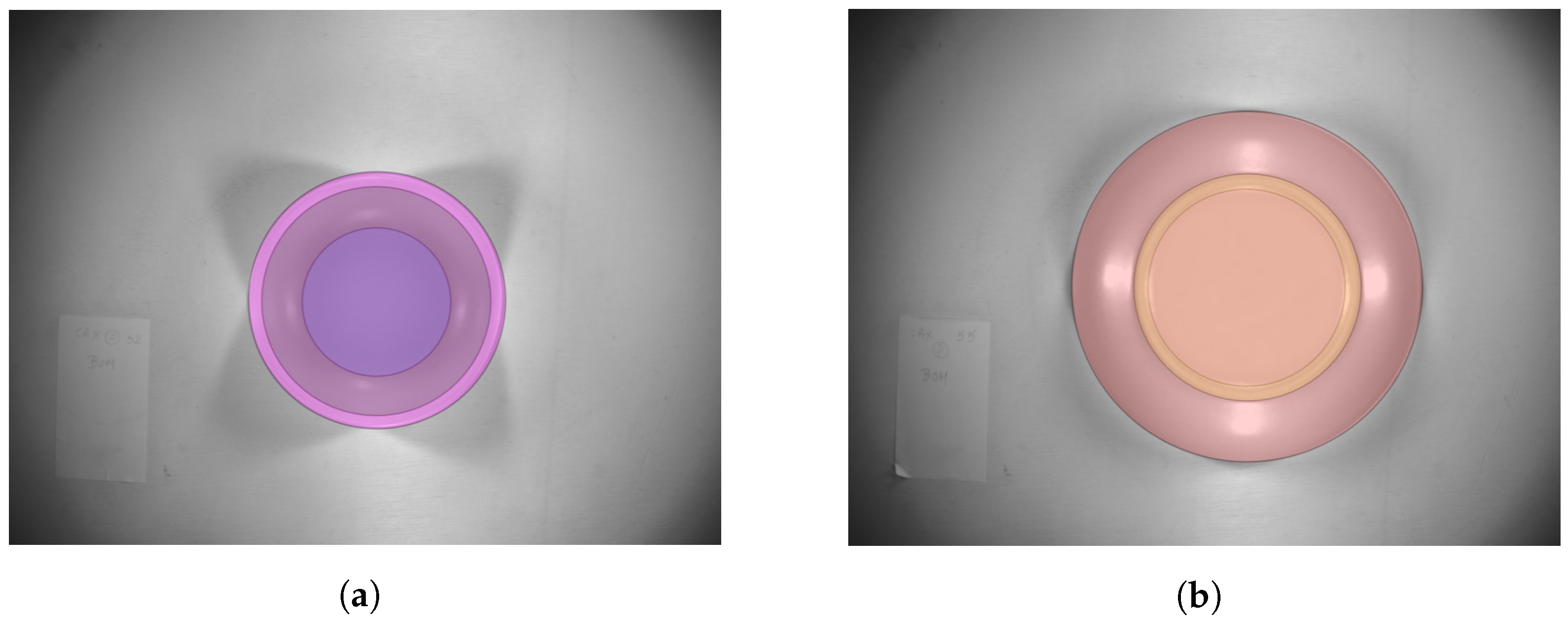
In Figure 4, it is possible to find two different pieces of tableware (a flat plate—Figure 4d and a cereal bowl—Figure 4b) belonging to batch 3 of data. In these images, the defects annotated by specialists through the developed tool are highlighted in different colors. The annotations are converted to the bounding box format for training of the defect detection module (presented in Section 3.5) The boxes are also used for cropping the regions of interest for defect classification (Section 3.6).
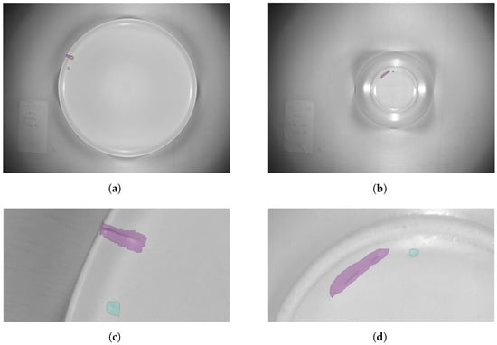
Figure 4.
Examples of defects annotated by specialists. Images belong to batch 3 of data. The blue regions correspond to class Defect-11 and the purple regions are examples of Defect-12. (a) Plate with “cracked” and “pore” defects; (b) Bowl with “cracked” and “pore” defects; (c) Zoom view of plate with the same defects; (d) Zoom view of bowl with the same defects.
3.3. Piece Zone
Each tableware ceramic piece is characterized by zones according to utility or design. Since the location of a defect in a given zone influences the quality and, consequently, the market value of the piece, it is important to have an automatic method for piece zone detection. To identify the relevant zones in the ceramic piece, we experimented with multiple networks within the MMSegmentation framework [17]. This open-source semantic segmentation toolbox, built on PyTorch, allows us to utilize state-of-the-art neural networks and a wide range of augmentation libraries. During our experimentation, we tested two different backbones with the DeepLabV3+ [18] semantic segmentation architecture: ResNet18 [19] and ResNet50 [20]. However, after evaluating their performance, we swiftly discarded the ResNet18 backbone due to its inferior results compared to the ResNet50 backbone. Consequently, we proceeded with the more effective ResNet50 backbone for our semantic segmentation process.
3.3.1. Data Processing
Since the tableware used in this dataset are all of circular shape (see Figure 5), we annotate the different piece zones of the tableware piece with a circular or ellipse form, using the developed internal tool of annotation. One tableware piece (two images front and back) can have up to seven zones of interest for defect priority categorization in the quality control. After completing these annotations, we prepared a script to do offline data augmentation that includes Gaussian noise addiction, motion blur, and elastic transformations. Therefore, in this phase, the training set contains 1718 images and the test set 786 images.

Figure 5.
Examples of zones annotated by specialists. The most saturated purple color to the less saturated regions correspond, respectively, to the center top zone, lateral top zone, and border. Similar for the bottom part of the bowl, the annotated zones are the center bottom zone, foot-ring, and lateral bottom zone, respectively, from the center of the bowl to the outside part of the bowl. (a) Cereal bowl front zones annotated; (b) Cereal bowl back zones annotated.
3.3.2. Training Details
For the training process, we followed the same structure of the config sample provided by the framework and adjusted it for this use case in particular. The major modifications were setting the number of classes as, in this case, seven classes were used, setting the total number of steps to be trained to 80,000, the batch size to 4, and the input size to . We used the cross entropy loss with the SGD optimizer, considering a learning rate of 0.01 and a momentum of 0.9 while decaying the learning rate from 0.01 to 0.0001 in 8000 steps using the polynomial decay function with a power of 0.9.
3.4. Anomaly Detection
Anomaly detection concerns the task of identifying instances that significantly differ from the majority of the samples in a given distribution. It may then be used as a means of validation, consisting of an essential step in various decision systems [10].
In this experiment, the fast AnoGAN (f-AnoGAN) [14] framework was explored in order to identify possible defects in data and the corresponding degree of abnormality. The choice of this framework had to do not only with its capacity to process images by patches [14], as intended in this work, but also with the promising results that we previously achieved with it in exploratory studies from other domains, such as industry or healthcare.
3.4.1. Data Processing
To address the challenge posed by the small dimensions of defects found in the dataset, which could potentially disappear when resizing images, a strategy of dividing the images into patches was employed. In this procedure, different sizes were explored, namely by diving images in patches of and pixels. The overlap between patches was also set to 50% and to 10%. Nevertheless, we verified that when patches of or an overlap of 50% were considered, the number of patches without defects was substantially higher, so it was decided to proceed with patches of pixels, using an overlap of 10%.
Furthermore, to train the anomaly detection framework, only patches without defects (belonging to batches 1, 2, 3, and 4 of images) have been selected in order to teach the models the different variations that a normal sample may exhibit. Therefore, 70% of the patches without defects from set 1 were used to train the algorithm and the remaining 30%, together with all the defects (from 13 different classes) contained in the dataset, were used to test the framework, forming test set 1. The evaluation comprised yet another test set (test set 2) where a completely new set of images collected in a different time frame (batches 5 and 6) was introduced in order to evaluate the robustness of the developed anomaly detector. Test set 2 then includes all patches from test set 1 and the new dataset that is composed of patches without defects (normal samples) and with defects belonging to 15 different classes.
3.4.2. Training Details
f-AnoGAN consists of a framework specifically designed for anomaly detection, and is composed of a Generative Adversarial Network (GAN) and an Encoder, which are trained in different steps. One particularity of this framework is that it can be applied to any pre-trained GAN. Therefore, in this work, a DCGAN [21] was employed to learn a non-linear mapping function from the latent space, Z, to the image space that represents the variability of (normal) training images. With respect to the Encoder architecture, the network was composed of five dense layers.
To train the GAN, a total of 300 epochs was performed. The binary cross-entropy was considered and the Adam optimizer with a learning rate of was used. The dimensionality of the latent space was set to 100. Regarding the training process of the Encoder, 300 epochs were also made and the Adam optimizer with a learning rate of was considered.
3.4.3. Evaluation
In order to evaluate the performance of the developed anomaly detection framework, three different metrics were computed, namely the Image Distance, Anomaly Score, and Z-distance. The corresponding definition is described below:
- Image Distance: consists of the Mean Squared Error (MSE) between the real image and the fake image (i.e., image generated by GAN);
- Anomaly Score [14]: is the deviation between the query images and corresponding reconstructions, which is given by: , where x is a new image, is the image distance, is the MSE between the features extracted from the real and the fake images, and k is a weighting factor, which, in this work, was set to one;
- Z-distance: corresponds to the MSE between the real and the fake latent spaces.
3.5. Defects Detection
For the defect detection model, we experimented with three state-of-the-art object detection models, namely YOLOv5 and YOLOv8 from the YOLO (You Only Look Once) framework, and RetinaNet [19] with a ResNet50 [20] backbone from the TensorFlow Object Detection API.
YOLO is a real-time object detection model that offers high accuracy and efficiency by directly predicting bounding boxes and class probabilities from a single neural network pass. YOLO divides the input image into a grid and assigns each grid cell the responsibility of detecting objects present within its boundaries. Each cell predicts bounding boxes and corresponding class probabilities based on predefined anchor boxes.
RetinaNet is an object detection framework that operates as a one-stage detector and tackles the challenge of class imbalance during training by employing a focal loss function. The ResNet50 backbone serves as the feature extractor in RetinaNet. It is a deep convolutional neural network architecture that comprises multiple residual blocks. These residual blocks enable the model to effectively capture and represent rich, hierarchical features from input images.
3.5.1. Data Processing
The previously described approach of dividing the images in patches generated the inputs for this module as it ensures that the defects are adequately captured and preserved, allowing for more accurate detection and analysis within the defect detection model. The overlap between patches was set to 50% to guarantee that an entire defect was present in the selected area (except for the Defect-12 class which presented bigger dimensions in some cases, as it represents cracked pieces).
Offline data augmentation techniques were also performed to enhance the model’s generalization and robustness. The generation of additional image data by applying transformations in contrast, brightness and sharpness, and adding Gaussian and motion blur helps to increase the diversity of the training data.
3.5.2. Training Details
We tested different YOLO variants—YOLOv5m, YOLOv5l, YOLOv8m, and YOLOv8l—which differ in architecture and size, and offer a trade-off between model size and performance. The models were trained for 200 epochs, with an input size of .
We fine-tuned the RetinaNet model, with weights pre-trained on the COCO 2017 dataset, for our specific case, using the Adam optimizer with an exponential decay learning rate. The input images are resized to .
The training parameters adopted in the experiments with both frameworks were specified in their respective original configuration files.
3.6. Defects Classification
The defect classification model was based on the EfficientNet-B3 architecture, a state-of-the-art deep learning model known for its efficiency and accuracy.
3.6.1. Data Processing
There is an insufficient amount of data available for specific defects compared to other more commonly found defects. For this reason, we compiled similar defects into broader categories, resulting in a reduced number of classes (9). However, there is still class imbalance which can lead to overfitting of the classification model, thus reducing generalization. To address this issue, data augmentation techniques were employed, namely translations, rotations, flips, blurring, contrast, and sharpness adjustments. Furthermore, we used a weighted loss function to assign higher weights to the underrepresented classes and lower weights to the overrepresented classes.
3.6.2. Training Details
To adapt the EfficientNet-B3 architecture for our defect classification task, we modified its final fully connected layer to output the probabilities for the number of defect classes present in our dataset. The model’s parameters were optimized through stochastic gradient descent (SGD) with a learning rate of , and it was trained for 300 epochs with an input size of . The training parameters were chosen based on empirical determination, after conducting multiple experiments.
4. Results
4.1. Piece Zone
To respond to aim 3 of this work (outlined in Section 1), in order to evaluate the performance of the segmentation of piece zones, we computed the Intersection over Union (IOU) and accuracy for each zone. The central top zone is the most relevant for quality control purposes, while the central bottom zone is the less relevant to this end. In Table 2, it is possible to find the values of such metrics for each class, and the mean IOU and accuracy.
Table 2.
Test set metrics obtained for the piece zone segmentation task.
4.2. Anomaly Detection
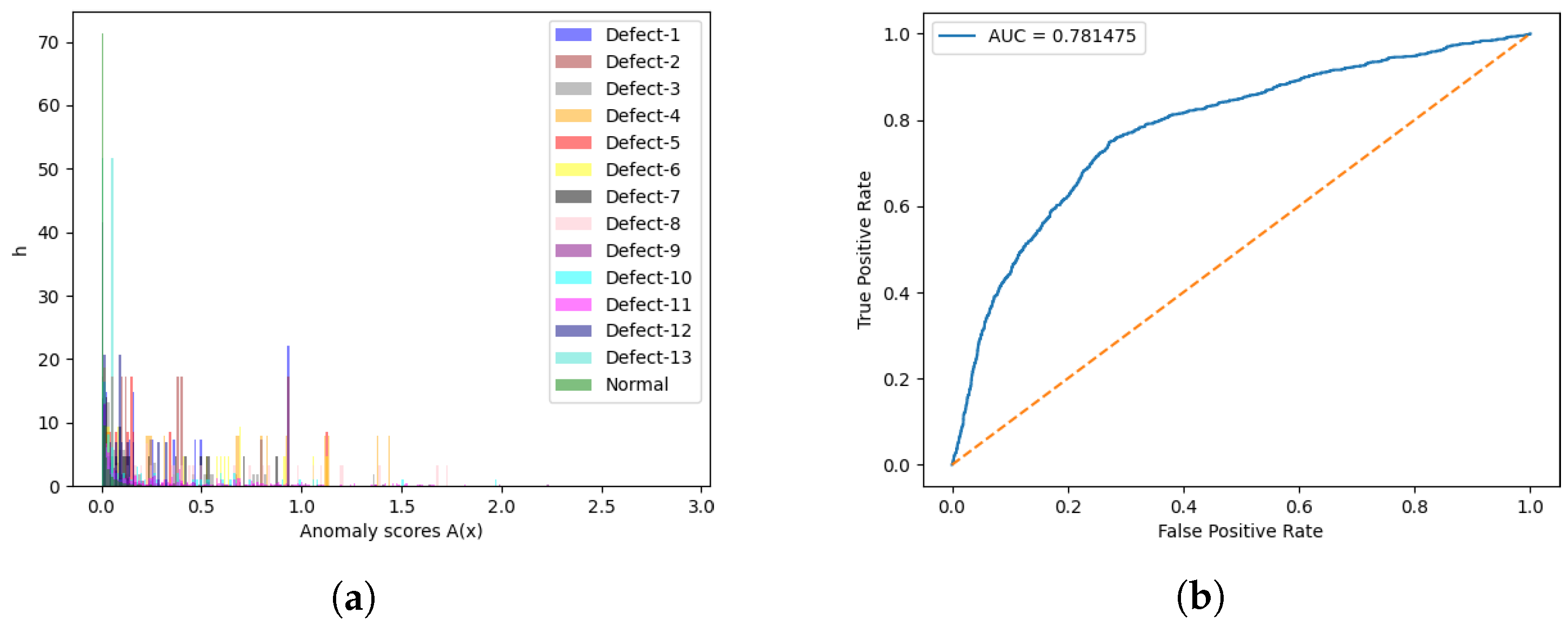
To evaluate the performance of the anomaly detector, for each test sample, three metrics were computed: the image distance of the generated image to the original image, the anomaly score, and the z-distance, which are defined in Section 3.4.3. In Table 3, it is possible to find the average values of such metrics for each class of test set 1, while in Figure 6a, the discrete distributions of the obtained anomaly scores are presented.
Table 3.
Average of the metrics obtained for the anomaly detector for each class of test set 1.
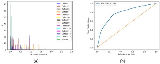
Figure 6.
Results for the anomaly detection engine with test set 1. (a) Discrete distributions of anomaly scores; (b) ROC-AUC curve in terms of anomaly scores.
As it is possible to infer from these results, the normal class, which corresponds to the images without any defect, achieved the lowest values in terms of the three computed metrics for almost all classes, with the exception of class 13 concerning the anomaly score metric. It is important to mention that, for these experiments with the anomaly detector engine, class Defect-13 was only present in two patches. Moreover, although these metrics are very close between some defective classes, which prevents their separability, the results suggest that this approach is able to distinguish between samples with and without (normal samples) defects. This statement may also be verified in Figure 6a, where the green (normal) samples are essentially settled in the leftmost area of the plot, which corresponds to the lowest anomaly scores, whereas for other defective classes, it is difficult to find the corresponding boundaries, due to the verified overlap.
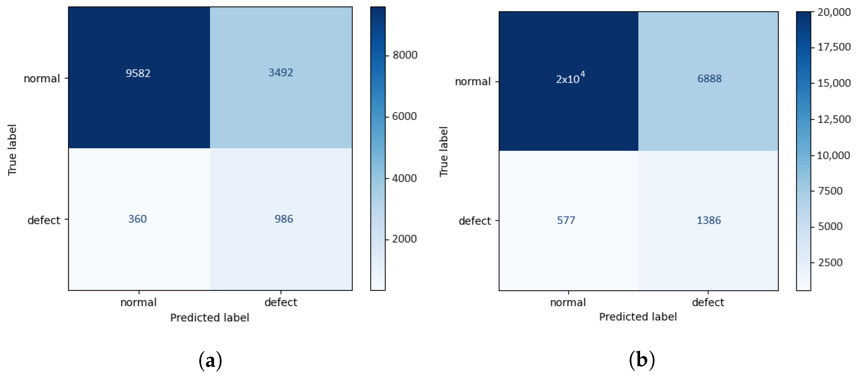
Bearing this in mind, a threshold was defined in order to distinguish between normal and defective samples. To establish this value, the ROC–AUC curve (Figure 6b) concerning the anomaly scores of test set 1 was plotted and the cut-off point, i.e., the closest point of the curve to the top left corner of the plot, was set as the threshold value, corresponding to an anomaly score of 0.0128. This was made using only test set 1, as it is composed of defective and normal patches that belong to the same set of images used to train the models but that have not been seen during the training process. Also, we decided to go with the anomaly scores to make this experiment as this metric was proposed in the original paper of f-AnoGAN [14] and gives information regarding the degree of anomaly. Therefore, a sample whose anomaly score is higher than this value is defined as a defective sample. The resulting accuracy, macro-average, and weighted-average metrics were then calculated for both test set 1 and test set 2, and the corresponding confusion matrices were computed, giving rise to the results shown in Table 4 and Figure 7, respectively.
Table 4.
Results of defect detection using the anomaly detection engine. Test set 1 refers to test images from batches 1, 2, 3, and 4; test set 2 comprises test set 1 and the entirety of batches 5 and 6.
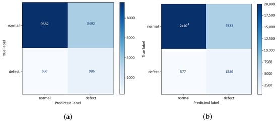
Figure 7.
Confusion matrices regarding defects detection using the anomaly detector engine. (a) Confusion matrix for test set 1; (b) Confusion matrix for test set 2.
These results show that the introduction of patches belonging to a dataset acquired in a different time window (test set 2) slightly penalized the macro-average metrics, which treat the two classes equally while improving the weighted-average metrics, which take into consideration the number of samples belonging to each class. It is worth noting that this new set of images that is present in test set 2 is essentially composed of patches without defects. By scrutinizing these outcomes in terms of classes, we verified that, overall, the ability of the framework to differentiate defective patches decreased, while its ability to detect normal patches improved. This may also result from the different acquisition conditions of these new samples, which may have influenced the defects’ appearance, even if minimally.
4.3. Defects Detection
The results presented in Table 5 indicate the performance of different defect detection models in both tests sets, comprising 289 and 619 defects, respectively.
Table 5.
Results of experiments for defect detection. Test set 1 refers to test images from batches 1, 2, 3, and 4; test set 2 comprises test set 1 and the entirety of batches 5 and 6.
The results demonstrate the superior performance of YOLO models compared to RetinaNet. RetinaNet achieved mAP@.5 below 30% in both sets, indicative of its difficulties to correctly identify defects. The best performing approaches are the YOLOv5 models, which yielded mAP@.5 scores of around 97% and 56% in test sets 1 and 2, respectively. The two variants of YOLOv8 achieved comparable results, but fell short when compared to alternative YOLOv5 models. It is worth noting that all YOLO models were trained using identical settings and hyperparameters. This difference in performance can potentially be attributed to the initial selection of well-suited anchor boxes using genetic algorithms, a step employed specifically in YOLOv5.
The discrepancy observed in the results between test set 1 and test set 2 can be attributed to data drift, due to the inclusion of images acquired at different time frames and under slightly varied conditions in the second set. These differences highlight the limited robustness of the model in accommodating minor variations. Additionally, inconsistencies in the ground truth annotations could also contribute to the contrasting outcomes. Therefore, it is evident that the models’ performance is impacted by the variations in image acquisition conditions as well as the consistency of the ground truth annotations.
Overall, considering the computational cost of the models, YOLOv5m appears to be the most effective model, as it delivers the best trade-off between performance and size.
4.4. Defects Classification
The defect classification model results are summarized in Table 6. This table presents key metrics and performance indicators associated with the classifier’s performance: accuracy rates and F1-score.
Table 6.
Results of the defect classification model. Test set 1 refers to test images from batches 1, 2, 3, and 4; test set 2 comprises test set 1 and the entirety of batches 5 and 6.
Classes Defect-10 (“Dots”) and Defect-12 (“Cracked”) present the highest F1-scores in both test sets, indicating successful classification. Despite the efforts to handle class imbalance, this behaviour was expected as the two classes of defects are the most represented. On the contrary, classes such as Defect-2, 4, 7 + 8 and 9 underperform, suggesting challenges in accurately identifying instances of those defects.
In terms of overall results for test set 1 and 2, the defect classification model achieved a macro accuracy of 89.97% and 77.00%, and F1-score of 74.66% and 59.90%, respectively. As explained in the previous section, the results of the first set outperform the second one because the model was trained in images acquired in the first batch of images. Nevertheless, the difference is not as abrupt as in the defect detection model, indicating more robustness and generalization capability of the classification model.
4.5. Pipeline
In accordance with the expected contributions of this work (aim 1 and 2, outlined in Section 1), this section provides the results of using end-to-end pipelines for defect identification.
Table 7 and Table 8 offer a comparison between the inference times (in seconds) and results, respectively, of two distinct pipelines: Pipeline A, which does not incorporate anomaly detection, and Pipeline B, which does include anomaly detection. The differentiation allows for a rigorous assessment of the performance differences between the two approaches, shedding light on the potential advantages and drawbacks of incorporating anomaly detection in the pipeline. The values presented in the tables were obtained by computing measurements on multiple batches of data and subsequently averaging the results.
Table 7.
Average inference times for each module of the vision pipeline. Pipeline A: Defect Analysis; Pipeline B: Anomaly-Driven Defect Analysis.
Table 8.
Average results of the vision pipeline. All values correspond to macro metrics. Pipeline A: Defect Analysis; Pipeline B: Anomaly-Driven Defect Analysis.
Pipeline A (with no anomaly detector) achieves defect characterization within approximately 7 s, thereby providing a baseline for inference time. In contrast, the alternative pipeline offers a reduction in defect detection inference time by minimizing the number of patches fed to the module through the adoption of patch selection with anomaly detection. However, this comes at the expense of a longer anomaly module runtime of 9 s due to the involvement of three models: a generator, a discriminator, and an encoder. Consequently, the alternative pipeline’s overall inference time amounts to 12 s. Comparing the two pipelines, it is evident that Pipeline A exhibits a faster inference time, outperforming the alternative pipeline by 5 s.
A decline in performance is evident for both vision pipelines with the metrics previously presented, attributed to the propagation of errors. Thus, a true positive in this case must be a piece with all the defects verified in the right location, with the correct type detected in the correct subzone of the piece. The general decline in performance is further amplified with anomaly detection, as the inclusion of an additional step aggravates the effect. The rationale behind incorporating this module was to effectively reduce the number of false positives identified by the defect detection process. However, the introduction of anomaly detection inadvertently leads to misclassification of patches containing defects as “defect-less” patches. As a consequence, besides the reduction in false positives, the number of true positives also gets adversely affected. This phenomenon highlights the inherent challenges and trade-offs associated with the application of anomaly detection in defect detection pipelines.
5. Conclusions and Future Work
Ensuring robust quality control processes in the ceramics industry is crucial to maintaining product excellence and customer satisfaction while minimizing defects and production costs. Nowadays, quality control protocols in this industry entail a rigorous, repetitive, subjective, and error-prone human manual inspection. The aim of this work was, therefore, to develop a semi-automated visual inspection framework designed for application on the shop floor that is able to detect the presence of defects in tableware pieces.
To achieve this goal, two pipelines were developed. For both of them, the first component comprised a piece zone detector, employing the DeepLabV3+ meta-architecture with a ResNet50 backbone (selected due to its higher performance), which is able to identify the relevant zones of the ceramic piece and so select the region of interest to be analysed by the following components. The difference between both pipelines essentially relied on the incorporation of an anomaly detection component based on the f-AnoGAN framework in order to pre-select possible defective patches. In one of the pipelines (Pipeline A), all patches coming from the piece zone detector were provided to a defects detector, whereas in the other (Pipeline B), only the patches identified as defective by the anomaly detector went on to the defects detector module. For this component, three state-of-the-art object detection models were used, namely YOLOv5, YOLOv8, and RetinaNet with a ResNet50 backbone. YOLO models demonstrated the superior performance in comparison to the RetinaNet, being YOLOv5m the most effective model. After the defects detection phase, the identified regions passed through a defects classification model derived from the EfficientNet-B3 architecture able to recognize different types of defects.
Each component was first evaluated before being integrated into each pipeline. The evaluation was made using two different sets of data. Test set 1 consisted of images sourced from the same batches of data used for model training, while test set 2 incorporated the images from test set 1 supplemented by new ones acquired in a different time frame of manufacturing production. The observed performance decrease in test set 2, resulting from the inclusion of the previously mentioned two additional data batches, aligns with expert feedback indicating the increased complexity of the recent data due to varying defect appearances, which could have led to subjective annotations. Moreover, it was also evident that critical defects lacked a sufficient number of representative samples, and only the “Dots” and “Cracked” defect types presented a high classification performance, with an accuracy of around 91% and 89%, respectively, and an F1-score of around 86% for both classes, with respect to the largest test set (test set 2).
Regarding the comparison of both pipelines (i.e., with and without the anomaly detection component), a decline in performance was verified when the anomaly detector was integrated, especially in terms of recall and F1-score, which decreased from around 70% to 21%, and from 40% to 23%, respectively. This drop in the results may have resulted from an additional source of error propagation, since some defective patches were misclassified as flawless by the anomaly detector, thus not being considered by the defects detector.
Despite the average achieved results, it is worth noting that this work comprises a highly challenging task. Beyond the huge diversity in the appearance of defects belonging to the same class (which in some cases are poorly represented), the quality of images among the different batches of data also varied, especially for the last two batches. Moreover, tableware pieces represent highly reflective surfaces, which increase the complexity of the problem, being in line with aim 4 of this work (outlined in Section 1).
These factors influenced not only the quality of the annotations by the specialists but may have also led to data-drift, significantly impacting the performance of the trained models and revealing their poor ability to generalize among different data.
In future work, it could be interesting to use f-AnoGAN to provide region proposals about the location of a defect, as proposed in the original paper [14]. These coarse segmentations could then be further assessed through a subsequent classification approach, consisting of an alternative method to the defect detection step presented in our work. Moreover, although we have used the anomaly scores metric to establish the defective/normal threshold for the reasons previously stated in Section 4.2, this threshold could also be defined with the z-distance metric in mind, since it provided promising results in terms of the difference between the normal and defective classes.
Author Contributions
Conceptualization, R.C. (Rafaela Carvalho), A.C.M., J.G. and F.S.; methodology, R.C. (Rafaela Carvalho), A.C.M., J.G. and F.S.; data curation, R.C. (Rafaela Carvalho), A.C.M., J.G. and F.S.; implementation, R.C. (Rafaela Carvalho), A.C.M. and J.G.; writing—original draft preparation, all; writing—review and editing, F.S.; supervision, F.S.; funding acquisition, A.K., A.G.e.S.R., R.C. (Rui Carreira) and F.S. All authors have read and agreed to the published version of the manuscript.
Funding
This work was financially supported by the project Visual and Acoustics Inspection of Ceramics (VAICeramics), co-funded by Portugal 2020 framed under the Operational Programme for Competitiveness and Internationalization (COMPETE 2020), by Agência Nacional de Inovação and European Regional Development Fund under Grant POCI-01-0247-FEDER-069987.
Institutional Review Board Statement
Not applicable.
Informed Consent Statement
Not applicable.
Data Availability Statement
In light of involved manufacturing plant privacy concerns, the image datasets acquired with pieces of Matcerâmica used in the aforementioned study will remain private. However, the research team is currently undertaking efforts to create a new dataset that is based on similar data, with the aim of making it publicly available.
Acknowledgments
The authors thank Rui Neves and Regina Santos from Centro Tecnológico da Cerâmica e do Vidro (CTCV) and Idalina Eusébio, Célia Santos, Eugénia Ribeiro from Matcerâmica factory for their expertise as inspectors which was critical for the work.
Conflicts of Interest
The authors declare no conflict of interest.
References
- Optomachines. CV3G: Tableware Inspection Machine. 2020. Available online: https://optomachines.fr/home/ceramics/cv3g-tableware-inspection-machine (accessed on 29 September 2023).
- Sciotex. A Vision Inspection System for Large Parts & Products. 2020. Available online: https://sciotex.com/examples/plate-quality-inspection-system (accessed on 29 September 2023).
- RSIP Vision. Defect Detection in Ceramics. 2020. Available online: http://www.rsipvision.com/defect-detection-in-ceramics (accessed on 29 September 2023).
- SYSTEM Ceramics. Ceramic Quality Control Machines. 2020. Available online: https://www.systemceramics.com/en/ceramic-machines/quality-control (accessed on 29 September 2023).
- SACMI. Vision Systems for Ceramics. 2020. Available online: https://sacmi.com/en-US/Control-Vision-Systems/Vision-for-Ceramics (accessed on 29 September 2023).
- Tao, X.; Zhang, D.; Ma, W.; Liu, X.; Xu, D. Automatic metallic surface defect detection and recognition with convolutional neural networks. Appl. Sci. 2018, 8, 1575. [Google Scholar] [CrossRef]
- Song, K.; Hu, S.; Yan, Y. Automatic recognition of surface defects on hot-rolled steel strip using scattering convolution network. J. Comput. Inf. Syst. 2014, 10, 3049–3055. [Google Scholar]
- Alexey Grishin, BorisV, iBardintsev, Inversion, Oleg. Severstal: Steel Defect Detection, 2019. Available online: https://kaggle.com/competitions/severstal-steel-defect-detection (accessed on 25 September 2023).
- Tabernik, D.; Šela, S.; Skvarč, J.; Skočaj, D. Segmentation-based deep-learning approach for surface-defect detection. J. Intell. Manuf. 2020, 31, 759–776. [Google Scholar] [CrossRef]
- Xia, X.; Pan, X.; Li, N.; He, X.; Ma, L.; Zhang, X.; Ding, N. GAN-based anomaly detection: A review. Neurocomputing 2022, 493, 497–535. [Google Scholar] [CrossRef]
- Liu, K.; Li, A.; Wen, X.; Chen, H.; Yang, P. Steel surface defect detection using GAN and one-class classifier. In Proceedings of the 2019 25th International Conference on Automation and Computing (ICAC), Lancaster, UK, 5–7 September 2019; IEEE: Piscataway, NJ, USA, 2019; pp. 1–6. [Google Scholar]
- Lai, Y.T.K.; Hu, J.S.; Tsai, Y.H.; Chiu, W.Y. Industrial anomaly detection and one-class classification using generative adversarial networks. In Proceedings of the 2018 IEEE/ASME International Conference on Advanced Intelligent Mechatronics (AIM), Auckland, New Zealand, 9–12 July 2018; IEEE: Piscataway, NJ, USA, 2018; pp. 1444–1449. [Google Scholar]
- Di, H.; Ke, X.; Peng, Z.; Dongdong, Z. Surface defect classification of steels with a new semi-supervised learning method. Opt. Lasers Eng. 2019, 117, 40–48. [Google Scholar] [CrossRef]
- Schlegl, T.; Seeböck, P.; Waldstein, S.M.; Langs, G.; Schmidt-Erfurth, U. f-AnoGAN: Fast unsupervised anomaly detection with generative adversarial networks. Med Image Anal. 2019, 54, 30–44. [Google Scholar] [CrossRef]
- Schlegl, T.; Seeböck, P.; Waldstein, S.M.; Schmidt-Erfurth, U.; Langs, G. Unsupervised anomaly detection with generative adversarial networks to guide marker discovery. In Proceedings of the International Conference on Information Processing in Medical Imaging, Boone, NC, USA, 25–30 June 2017; Springer: Cham, Switzerland, 2017; pp. 146–157. [Google Scholar]
- Ramalho, B.; Silva, E.; Soares, F.; Gonçalves, J.; Carreira, R.; Gil, A. The Role of Human-Machine Collaboration in the Quality Control of Ceramic Tableware with Visual and Acoustics Inspection; SIGCHI, ACM: New York, NY, USA, 2023. [Google Scholar]
- Contributors, M. MMSegmentation: OpenMMLab Semantic Segmentation Toolbox and Benchmark. 2020. Available online: https://github.com/open-mmlab/mmsegmentation (accessed on 27 March 2023).
- Chen, L.C.; Papandreou, G.; Schroff, F.; Adam, H. Rethinking Atrous Convolution for Semantic Image Segmentation. arXiv 2017, arXiv:1706.05587. [Google Scholar]
- Lin, T.Y.; Goyal, P.; Girshick, R.; He, K.; Dollár, P. Focal loss for dense object detection. In Proceedings of the IEEE International Conference on Computer Vision, Venice, Italy, 22–29 October 2017; pp. 2980–2988. [Google Scholar]
- He, K.; Zhang, X.; Ren, S.; Sun, J. Deep residual learning for image recognition. In Proceedings of the IEEE Conference on Computer Vision and Pattern Recognition, Las Vegas, NV, USA, 27–30 June 2016; pp. 770–778. [Google Scholar]
- Radford, A.; Metz, L.; Chintala, S. Unsupervised representation learning with deep convolutional generative adversarial networks. arXiv 2015, arXiv:1511.06434. [Google Scholar]


Disclaimer/Publisher’s Note: The statements, opinions and data contained in all publications are solely those of the individual author(s) and contributor(s) and not of MDPI and/or the editor(s). MDPI and/or the editor(s) disclaim responsibility for any injury to people or property resulting from any ideas, methods, instructions or products referred to in the content. |
© 2023 by the authors. Licensee MDPI, Basel, Switzerland. This article is an open access article distributed under the terms and conditions of the Creative Commons Attribution (CC BY) license (https://creativecommons.org/licenses/by/4.0/).