Article

Comparison of the Performance of Convolutional Neural Networks and Vision Transformer-Based Systems for Automated Glaucoma Detection with Eye Fundus Images

by
Silvia Alayón
1,*,
Jorge Hernández
1,
Francisco J. Fumero
1,
Jose F. Sigut
1 and
Tinguaro Díaz-Alemán
2
1
Department of Computer Science and Systems Engineering, University of La Laguna, 38200 Santa Cruz de Tenerife, Spain
2
Department of Ophthalmology, Canary Islands University Hospital, 38320 Santa Cruz de Tenerife, Spain
*
Author to whom correspondence should be addressed.
Appl. Sci. 2023, 13(23), 12722; https://doi.org/10.3390/app132312722
Submission received: 7 October 2023 / Revised: 22 November 2023 / Accepted: 24 November 2023 / Published: 27 November 2023

Abstract

:
Glaucoma, a disease that damages the optic nerve, is the leading cause of irreversible blindness worldwide. The early detection of glaucoma is a challenge, which in recent years has driven the study and application of Deep Learning (DL) techniques in the automatic classification of eye fundus images. Among these intelligent systems, Convolutional Neural Networks (CNNs) stand out, although alternatives have recently appeared, such as Vision Transformers (ViTs) or hybrid systems, which are also highly efficient in image processing. The question that arises in the face of so many emerging methods is whether all these new techniques are really more efficient for the problem of glaucoma diagnosis than the CNNs that have been used so far. In this article, we present a comprehensive comparative study of all these DL models in glaucoma detection, with the aim of elucidating which strategies are significantly better. Our main conclusion is that there are no significant differences between the efficiency of both DL strategies for the medical diagnostic problem addressed.

1. Introduction

Glaucoma is a disease that damages the patient’s optic nerve and is the leading cause of irreversible blindness worldwide [1]. A patient with glaucoma may remain asymptomatic until the disease reaches very advanced stages of development, making early diagnosis difficult. For the same reason, the number of people affected is assumed to be much higher than the number of diagnosed patients [2].
The optic nerve head, or “optic disc”, is a structure located in the retina made up of various tissues (neural, vascular, and connective). Inside it is a depression called the “optic cup” (Figure 1). Glaucoma damages the optic nerve tissues, causing molecular and functional changes in this region. This results in alterations of the microcirculation, atrophy of nerve neurons, and an enlargement of the cup, leading to visual loss [2]. All these changes can be seen in fundus imaging or retinography, which makes this type of imaging useful for the diagnosis of glaucoma [3].
The visual study of these images is a very subjective and not always simple operation, especially in the most incipient cases of the disease. For this reason, automated methods such as Deep Learning (DL) algorithms can reduce costs and make fast and consistent predictions, helping the specialist in the diagnosis.
In recent years, these DL algorithms have had a high impact on medicine. When the problem being addressed involves image processing and classification, it is quite common to use Convolutional Neural Networks (CNNs). These networks are able to automatically extract the most relevant features of the image and take advantage of the available spatial information. For this purpose, they apply convolutional filters (kernels) to the images [4]. Each of these filters is adjusted during the training of the network to detect a particular feature on the image so that the first layers of the network detect simple features (edges, textures, etc.), and as it goes deeper, the filters of the last layers are able to recognise more complex features [5].
In medicine, the application of CNNs can be found in several fields: skin cancer [6], lung diseases [7], heart diseases [8], breast cancer [9], vascular diseases [10], etc. In the case of Ophthalmology, these CNNs have been widely used for the diagnosis of diabetic retinopathy [11], macular degeneration [12], cataracts [13], and glaucoma [14,15,16,17].
In relation to glaucoma, the performance of three well-known CNNs is studied in [14]. The three best-fit models have very similar performance, offering accuracy values around 98% for a particular dataset. Similarly, in [16], the authors study the efficiency of ten well-known CNNs, obtaining a balanced accuracy of 87.48% with the VGG19 architecture [18]. A comparative study of the efficiency of three well-known CNNs and an ensemble model that combines the individual predictions of these three models is presented in [15]. In the training stage of these systems, several experiments are performed using four separate public and private datasets and, finally, with all these datasets fused together. The ensemble model proves to be superior in all tests, with accuracy values in the range of 88–98%. In [17], a new CNN architecture is proposed, trained, and tested with two different retinography databases, and the efficiency achieved in both cases is compared, which is around 0.831 and 0.887 (Area Under de Curve—AUC values).
On the other hand, Transformers [19], a DL architecture initially designed for Natural Language Processing (NLP), have recently appeared. Their results in NLP have been spectacular, which has sparked interest in adapting them for image processing. These Transformers adapted to work with images are known as Vision Transformers (ViTs) [20,21,22]. Broadly speaking, the Transformers apply a mechanism called “attention”, which allows the model to focus on the most relevant parts of the input sentence, assigning each word a weight proportional to its importance. When this architecture is adapted to work with images instead of words, the inputs to the attention mechanism are now portions (patches) of the input image. When these patches are introduced into the system, the spatial information of the image is lost, so it is necessary to introduce a positioning system that identifies each patch (positional embedding).
In the literature, we can already find several works that process images using ViTs instead of CNNs, for example, in remote sensing [23], traffic sign classification [24], forest fire segmentation [25], etc. However, there are also proposals for hybrid systems, which combine CNNs and ViTs with the intention of exploiting the advantages of each method separately [26,27,28,29]. Transformers [30] and ViTs [31,32] are starting to be used in medicine due to the multimodal nature of the data used in this field, where both text and image can be useful for diagnosis. An extensive review of the application of Transformers in healthcare is presented in [32].
Focusing on the field of Ophthalmology, we can cite the first works using ViTs to aid in the diagnosis of diabetic retinopathy [33] and macular degeneration [34]. In the case of glaucoma, there are still very few studies [35,36]. It is also worth mentioning the residual ResMLP architecture. ResMLP models are based on Vision Transformers but replace the attention mechanisms with classical Multi-Layer Perceptron (MLP) networks [37]. They have been applied very recently in glaucoma detection [35]. In some of these works, it can be interpreted that ViTs can become more efficient than CNNs. However, it is difficult to find papers that really compare the performance of both systems comprehensively. The most complete review we have found is [38], but it is not in the field of medicine. In glaucoma detection, we can only cite [35,36,39].
The work [39] compares a ViT-based architecture, the DeiT model [27], and a well-known residual CNN, the ResNet50 [40]. They train the models with a dataset and subsequently test them on other datasets. Their experimental results show that the efficiency of DeiT is superior when classifying these external databases. A comparative study between the efficiency of four well-known CNNs, the original ViT model, and two variants of the original ViT architecture is presented in [36]. Three public databases are used together for the design of the training and test sets. The best accuracy values were obtained with the ViT architectures (accuracy values of 95.8% and 93.8%). However, the best AUC value, 0.987, was provided by a CNN, a VGG19 model. In [35], a comparison study collects the efficacy in glaucoma detection of eight different ViT-based models. The authors fuse nine datasets (public and private) to train and test the selected models. The best architecture is CaiT [26], with an accuracy value of 94.5% and an AUC value of 0.979.
The aim of this work is to perform a comprehensive comparative study between CNN and ViT models, hybrid systems, and ResMLP architecture for the problem of glaucoma detection with retinographies. In our research work, we have tried to include a wide variety of CNNs (VGG19 [18], ResNet50 [40], InceptionV3 [41], and Xception [42]), the base architecture of ViT [20], variations in ViT (Swin Transformer [21] and Twins-PCPVT [22]), several hybrid systems (CaiT [26], DeiT [27], CeiT [28], and ConViT [29]), and, also, the very recent residual architecture ResMLP [37].
For the training and testing of all these models, we have used images provided by the collaborating medical expert of the Canary Islands University Hospital together with images from Rim-ONE-DL [43], a publicly available glaucoma database. In addition, the efficiency of the models has been analysed using other public databases: Refuge [44], Drishti-GS1 [45], and Papila [46]. The inclusion of multiple datasets improves the reliability of the study results and contributes to a complete understanding of the efficiency of each DL system used.
This paper is organised as follows: first, we present the datasets we worked with, a brief description of all the DL models selected in the study, and an explanation of how the experiments were designed. Next, we present the experimental results obtained and a comparative study of them. Finally, the conclusions of the study are given.

2. Materials and Methods

This paper presents a comparative study of the efficiency of different DL models in the classification of retinographies for the diagnosis of glaucoma. Therefore, this section will present the retinography datasets used, explain the basic fundamentals of the selected DL models, and finally, detail the conditions under which the experiments were performed. Within the exposition of the models considered in this study, CNNs, ViTs, hybrid CNN-ViT systems, and ViT-inspired systems are distinguished.

2.1. Description of the Datasets

The dataset used to train and test the different DL models employed in this study is composed of:
  • The public database Rim-ONE DL [43] is composed of 172 images of glaucoma and 313 of normal eyes;
  • Fundus images were collected by the medical specialist of our research team, belonging to the Canary Islands University Hospital (Spain). This set is composed of 191 images of glaucoma and 63 of normal eyes. These images, which are not public, were acquired with the Topcon TRC-NW8 multifunctional non-mydriatic retinograph. This study was conducted in accordance with the Declaration of Helsinki and approved by the Research Ethics Committee of the Canary Islands University Hospital (CHUC_2023_41, 27 April 2023). Confidentiality of personal data was guaranteed.
A total of 739 images were used: 363 retinographies of glaucoma and 376 of normal eyes.
To perform a more thorough validation of the DL models, we used other publicly available databases:
  • The Drishti-GS1 database [45] consists of 101 images, of which 70 are classified as having glaucoma and 31 as having healthy eyes;
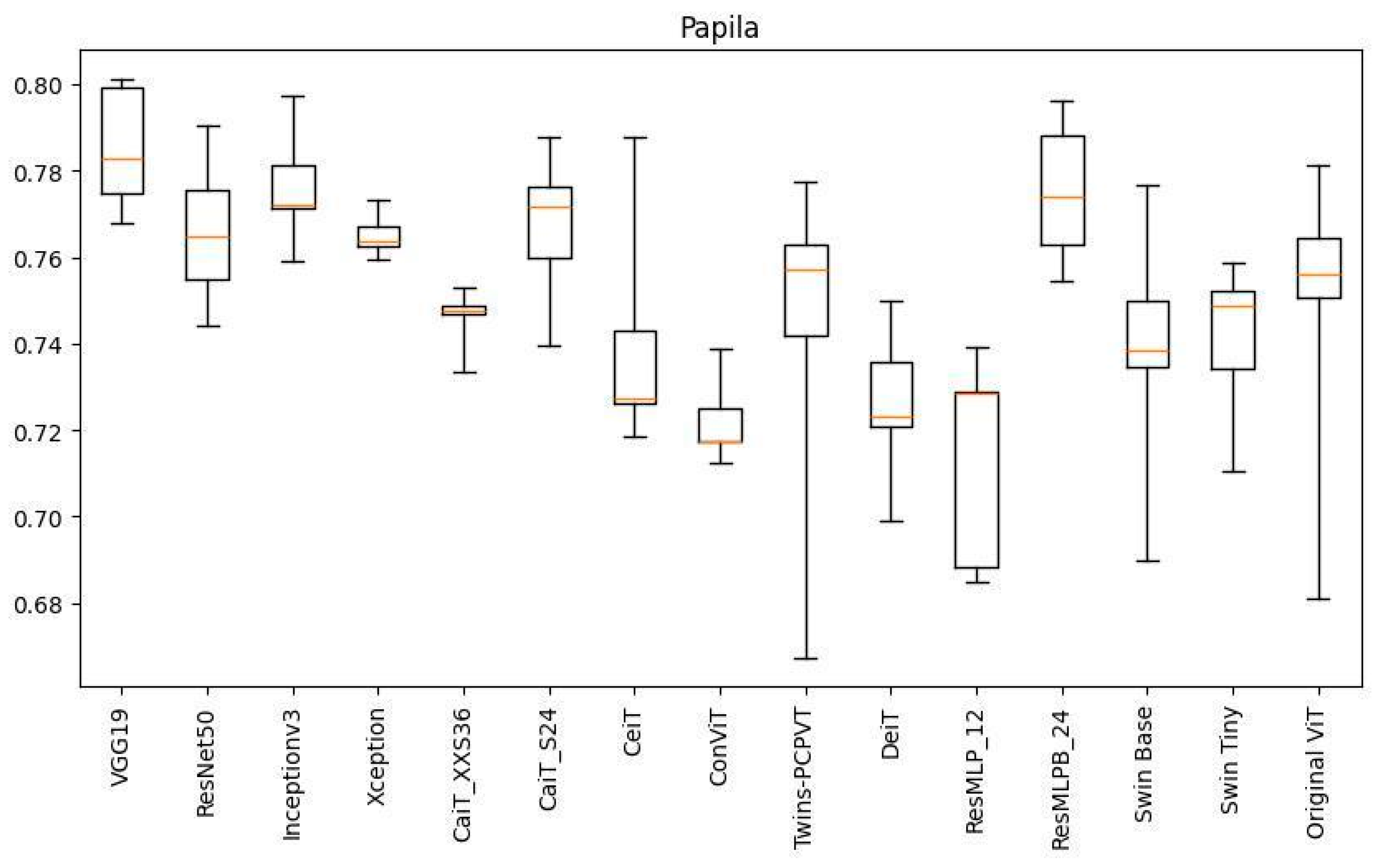
  • The Papila dataset [46] consists of 421 images, of which 87 are classified as having glaucoma and 334 as having healthy eyes;
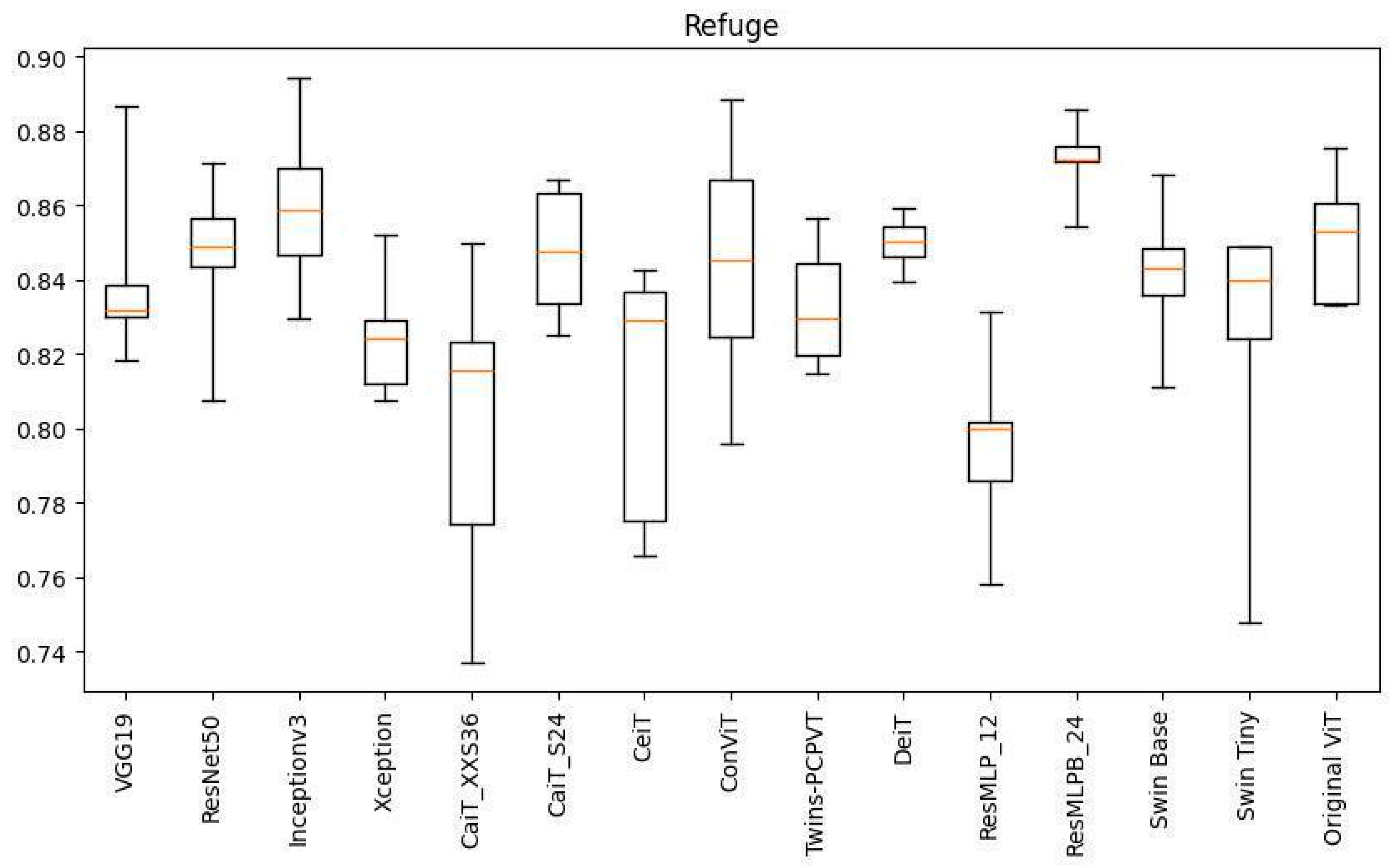
  • The REFUGE challenge database [44] consists of 1200 retinal images. Of the total dataset, 10% (120 samples) correspond to glaucomatous subjects.

2.2. Description of the Selected DL Architectures

CNNs and ViT-based systems have some differences that may make their application more appropriate in one scenario or another [38]. The most important ones are:
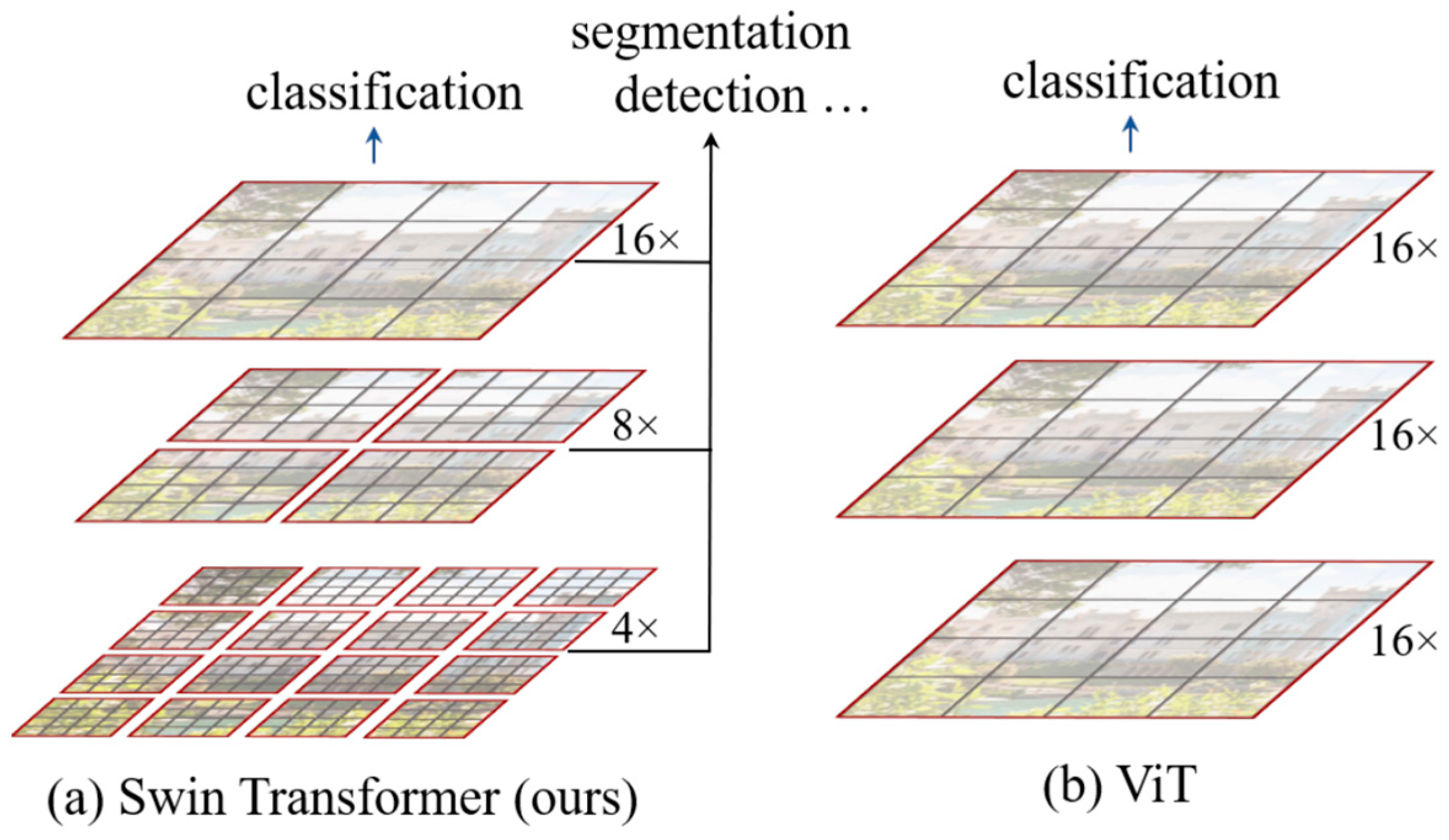
  • CNNs are designed to exploit local spatial correlations through the use of convolutional layers, which makes them effective at capturing local patterns and features in an image. In contrast, ViT-based systems employ an attention mechanism that allows them to capture global relationships between image patches, which makes these systems more suitable for handling long-range dependencies and capturing the global context of an image.
  • CNNs require a larger number of parameters, which makes them computationally expensive. ViTs take advantage of attention mechanisms to capture the global context more efficiently with fewer parameters. This can be advantageous when computing resources or memory are limited.
  • CNNs are intrinsically translation-invariant, thanks to the use of shared weights in the convolutional layers. This property is very useful for image classification. In contrast, ViTs do not have this inherent translation invariance due to their self-attenuation mechanism, although it can be incorporated by positional embedding.
  • Both CNNs and ViT-based systems have been shown to have a high generalisability capacity when trained on large datasets. In this sense, ViT-based systems are more sensitive to the size of the training set, as they tend to require larger sets than CNNs.
  • CNNs lack interpretability; it is difficult to understand how they make their decisions, and they are often used as “black boxes”. In that sense, the attention mechanisms of ViT-based systems are more useful, as they allow for analysing which parts of an image are more relevant when making predictions.
In the following subsections, we detail the most relevant features of all the DL models used in this study.

2.2.1. Convolutional Neural Networks

Convolutional Neural Networks (CNNs) are a type of neural network with a large number of internal layers specifically designed for image processing. They consist mainly of convolutional layers, which apply convolutional filters to the input images and learn local patterns in small, two-dimensional windows. The purpose of these layers is to detect features in the images (edges, color, texture, etc.). Once it learns to recognise a feature somewhere in the image, it is able to detect it anywhere in the image [5]. Another important aspect of CNNs is that convolutional layers can learn spatial hierarchies of patterns while preserving spatial relationships, so that features detected by one layer can be combined in subsequent layers to form more complex patterns.
There are several popular CNN architectures pre-trained with the Imagenet database available to the scientific community. In the present work, the VGG19 [18], ResNet50 [40], InceptionV3 [41], and Xception [42] networks have been selected. In the following, we briefly describe their fundamentals:
  • VGG19 contains 19 layers: 16 convolutional layers grouped into 5 blocks and 3 full connection layers [18]. After each convolutional block, there is a pooling layer that decreases the size of the obtained image and increases the number of convolutional filters applied (Figure 2). The dimensions of the last three full connection layers are 4096, 4096, and 1000, respectively, because VGG19 was designed to classify Imagenet images into 1000 categories;
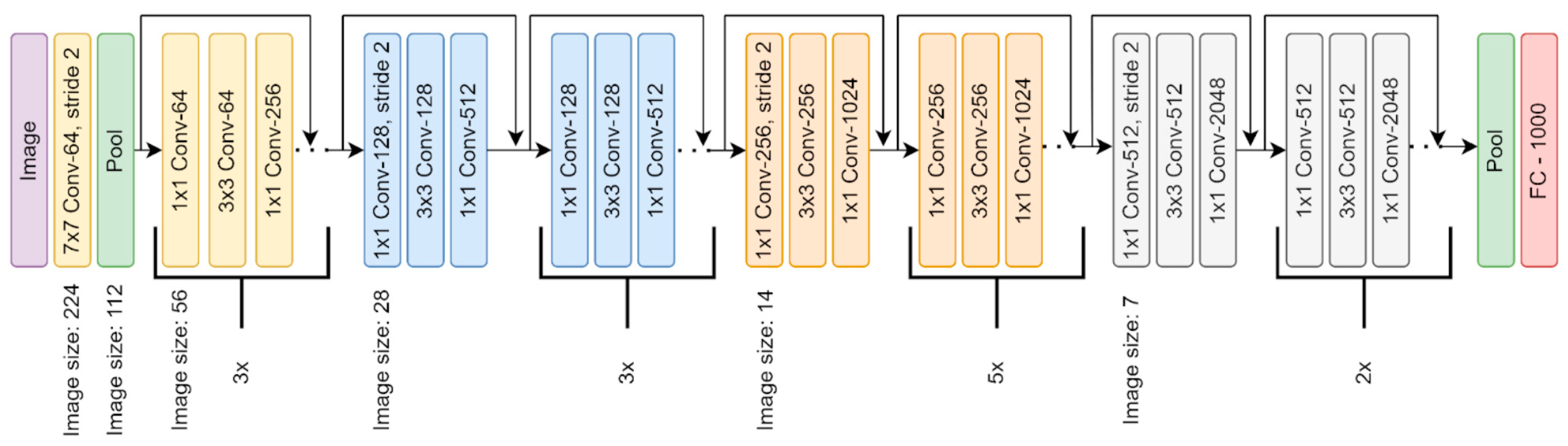
  • ResNet50 is a network that allows hops in layer connections to facilitate training and improve its performance. It consists of 49 convolutional layers, two pooling layers, and a full connection layer (Figure 3). The blocks that make up the network follow a bottleneck design that reduces the number of parameters and matrix multiplications [40];
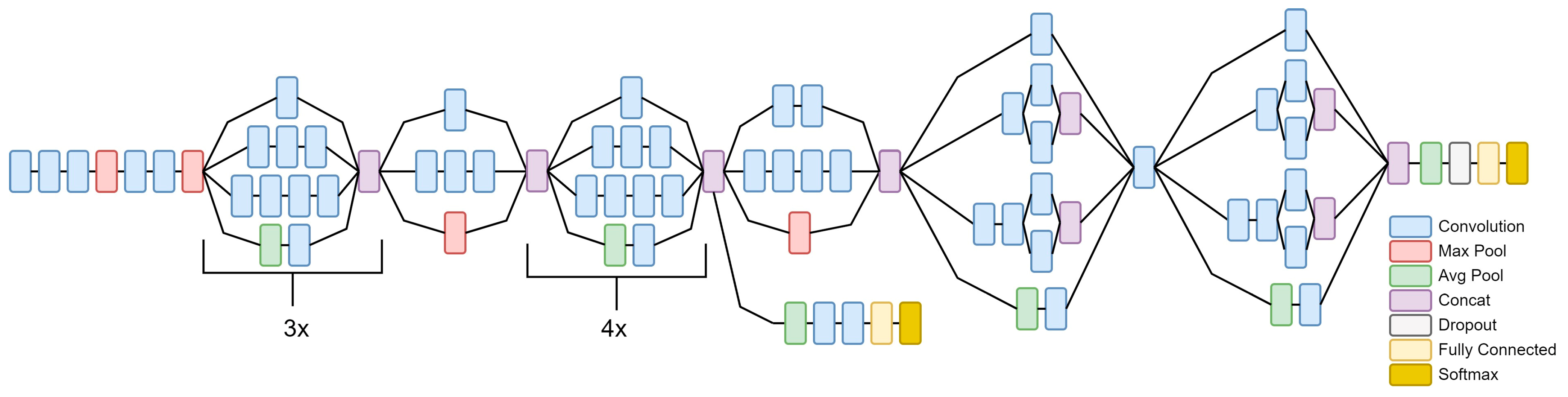
  • InceptionV3 consists of 48 depth layers combining convolutional, pooling, and fully connected layers with concatenation filters (Figure 4). The network is distributed in “spatial factorisation” modules, which apply different convolutional layers of different sizes to the input image to obtain general and local features. The concatenation filter combines the results provided by the spatial factorisation module into a single output, which will be the input of the next module [41];
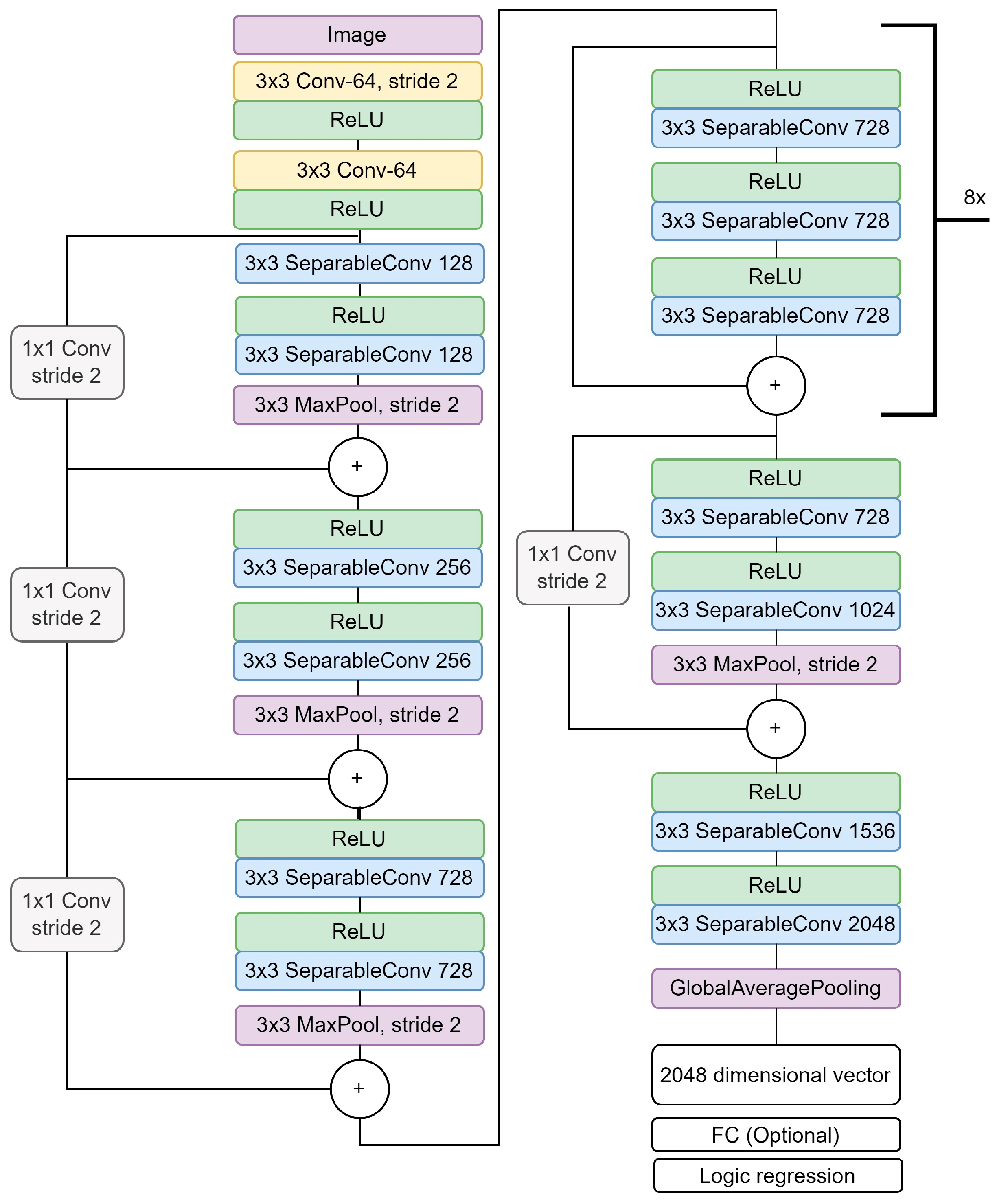
  • Xception is a variant of the Inception architecture that focuses on the use of separable convolutions instead of standard convolutions. Separable convolutions split the convolution operation into two stages: a first stage that performs convolutions on each input channel individually, followed by a linear combination stage that fuses the learned features [42]. The architecture of this network, which is 71 layers deep, is shown in Figure 5.
All these CNNs have been designed to classify, as efficiently as possible, the Imagenet images into 1000 classes. For this reason, the last full connection layer of all of them is composed of 1000 neurons. When applying these networks to other classification problems, it is necessary to change the dimension of this last full connection layer. For example, in our case, the last layer contains only two neurons because the retinal images are classified into two categories: “normal” and “glaucoma”.

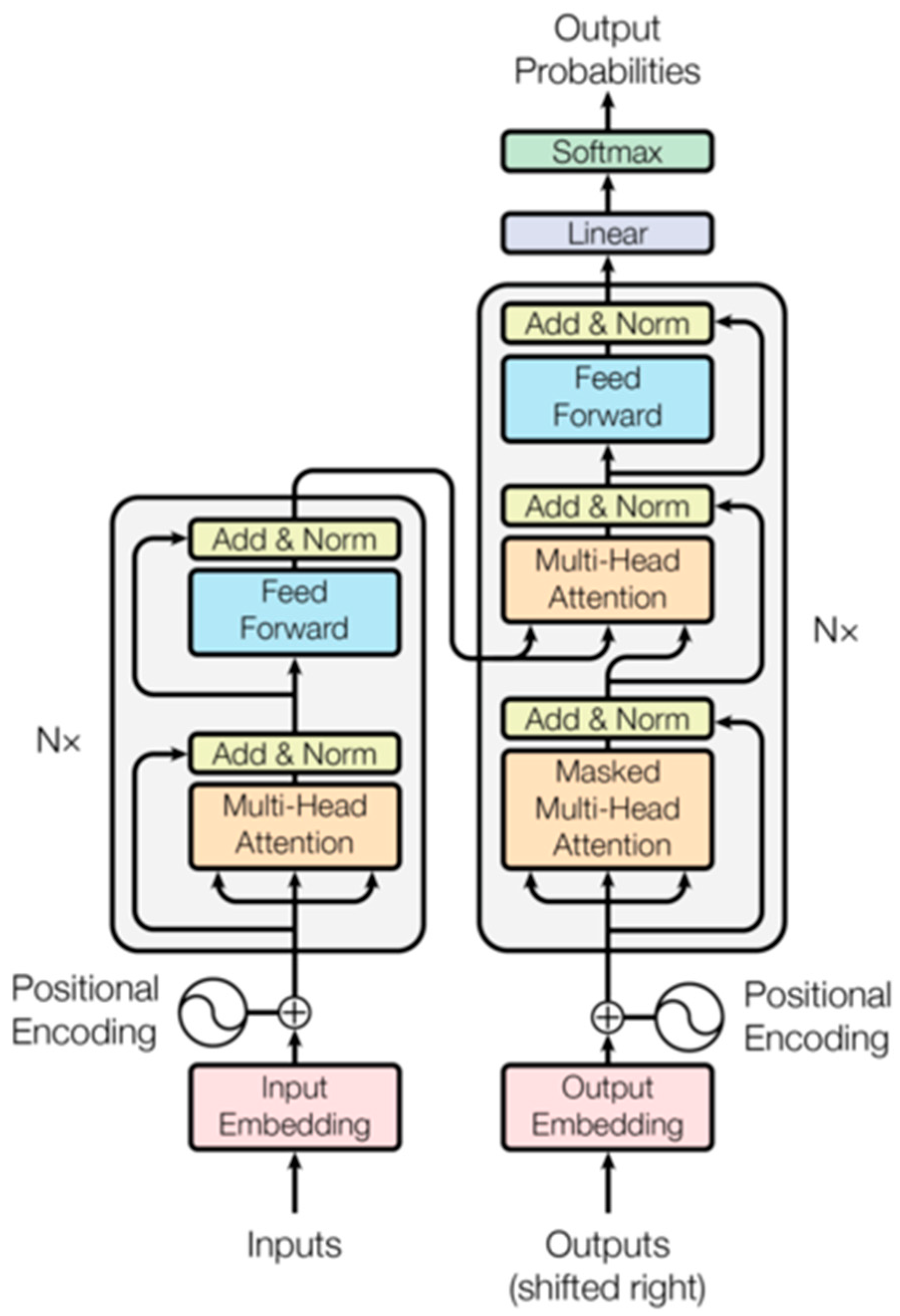
2.2.2. Vision Transformers

Transformers are DL systems that originally emerged to improve the performance of Recurrent Neural Networks (RNNs) in Natural Language Processing (NLP) tasks [19]. They were later adapted to image processing, giving rise to the recent Vision Transformers (ViTs) [20]. To understand the basic features of ViTs, it is necessary to know some fundamentals of Transformers.
Most classical text processing systems apply a sequential, word-by-word analysis strategy. This implies that the influence of the first words of a sentence can be lost if the text is very long. Transformers avoid this because they are able to analyse all words in parallel, retaining a measure of the position of each word in the sentence (positional encoding). Also, in order for the system to be able to work with the words, they are transformed into vectors in a semantic space, so that words with similar meanings have more similar and closer vectors [19]. This transformation of words into vectors allows the application of attention mechanisms, whose mission is to calculate the importance of each word within a sentence and how it relates to the rest of the words in the sentence. These mechanisms are included in Multi-Head Attention (MHA) layers, which are contained in the “encoder” and “decoder” blocks of the transformer. The basic structure is shown in Figure 6.
Vision Transformers (ViTs) are a variation of Transformers for image processing. The input image is divided into patches, which are processed by the system in parallel in the same way as transformers do with words (Figure 7). The positional encoding and the attention mechanisms described above are applied to these patches. An additional patch, called “token class”, is added to the image to perform the image classification. Vision Transformers have only encoder blocks [20].
In this paper, we have applied the original ViT [20] to the classification of eye fundus images for glaucoma diagnosis. In addition, we have also considered the inclusion in our study of two modifications of the original ViT called “Swin transformer” [21] and “Twins-PCPVT” [22].
The Swin Transformer [21] allows the windows of the attention mechanism to be scaled and shifted efficiently to reduce computational cost and improve performance (Figure 8). As the windows have neither a fixed size nor a fixed position, this architecture uses a relative positioning system instead of the absolute positioning used in the original ViT. In our comparative study, we tested two versions of this model: the “Swin Tiny” version, which has 96 layers and 28 million parameters, and the “Swin Base” version, with 128 layers and 88 million parameters.
The Twins-PCPVT model [22] also divides the image into patches or windows of variable size. In this case, the windows are progressively decreased in a pyramidal scheme. In addition, the attention mechanism is combined with the use of conditional position encodings (CPE) to replace the absolute positioning used in ViT. The Position Encoding Generator (PEG) is responsible for generating these conditional positionings (Figure 9). The use of the CPE is inspired by the Swin Transformer model explained above.

2.2.3. Hybrid Systems

Hybrid systems combine ViTs and CNNs with the aim of further improving image processing efficiency. In the hybrid system, local features are captured with CNNs, while more global relations are obtained with the attention mechanisms of ViTs. These systems have been included in the comparative study carried out in this work because they are increasingly used in the medical field.
Hybrid systems are very recent, but there are already several architectures trained with Imagenet and available to the scientific community. In the present work, DeiT [27], CaiT [26], CeiT [28], and ConViT [29] have been used. We describe them briefly below:
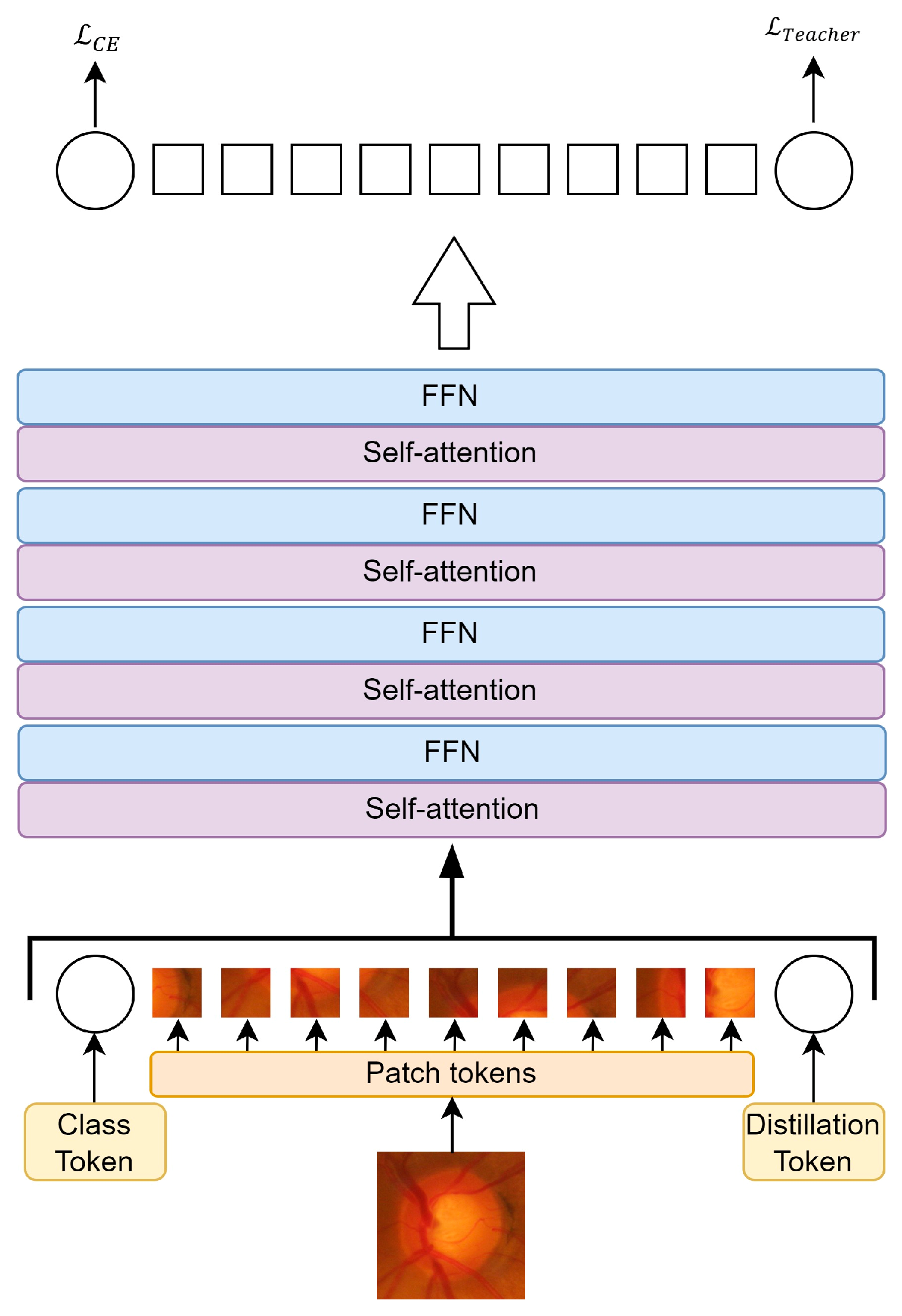
  • DeiT is a ViT trained with a transfer learning technique called “knowledge distillation” [27]. A larger convolutional model is used as a “teacher” to guide the training of the smaller model, which is the ViT part. For this purpose, the “distillation token” is introduced, and the goal of the ViT part is to reproduce this label instead of the class label (Figure 10);
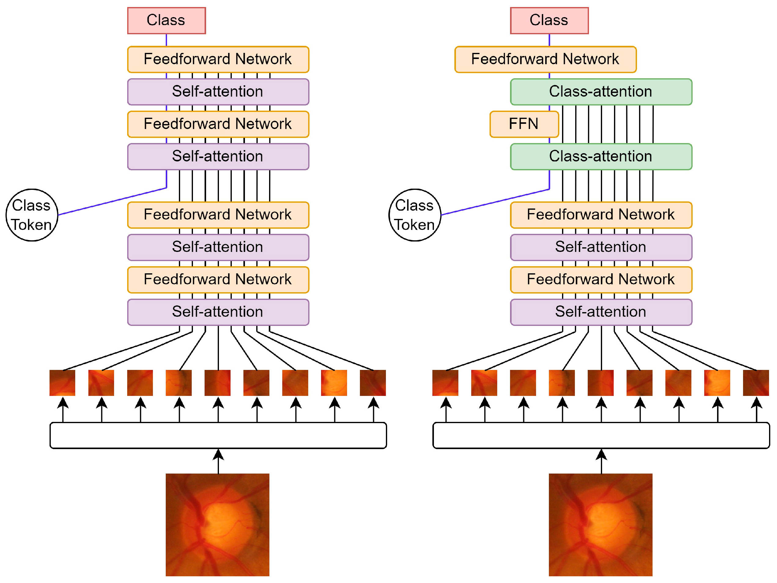
  • CaiT [26] is based on DeiT and also uses distillation training. In CaiT, a LayerScale normalisation is added to the output of each residual block, and new layers called “attention class” layers are incorporated. These layers allow the separate computation of inter-patch self-attention and classification attention to be finally processed by a linear classifier (Figure 11). In our work, we have tested two versions of this model: the “CaiT_XXS36” version with 17.3 million parameters and the “CaiT_S24” version with 46.9 million parameters;
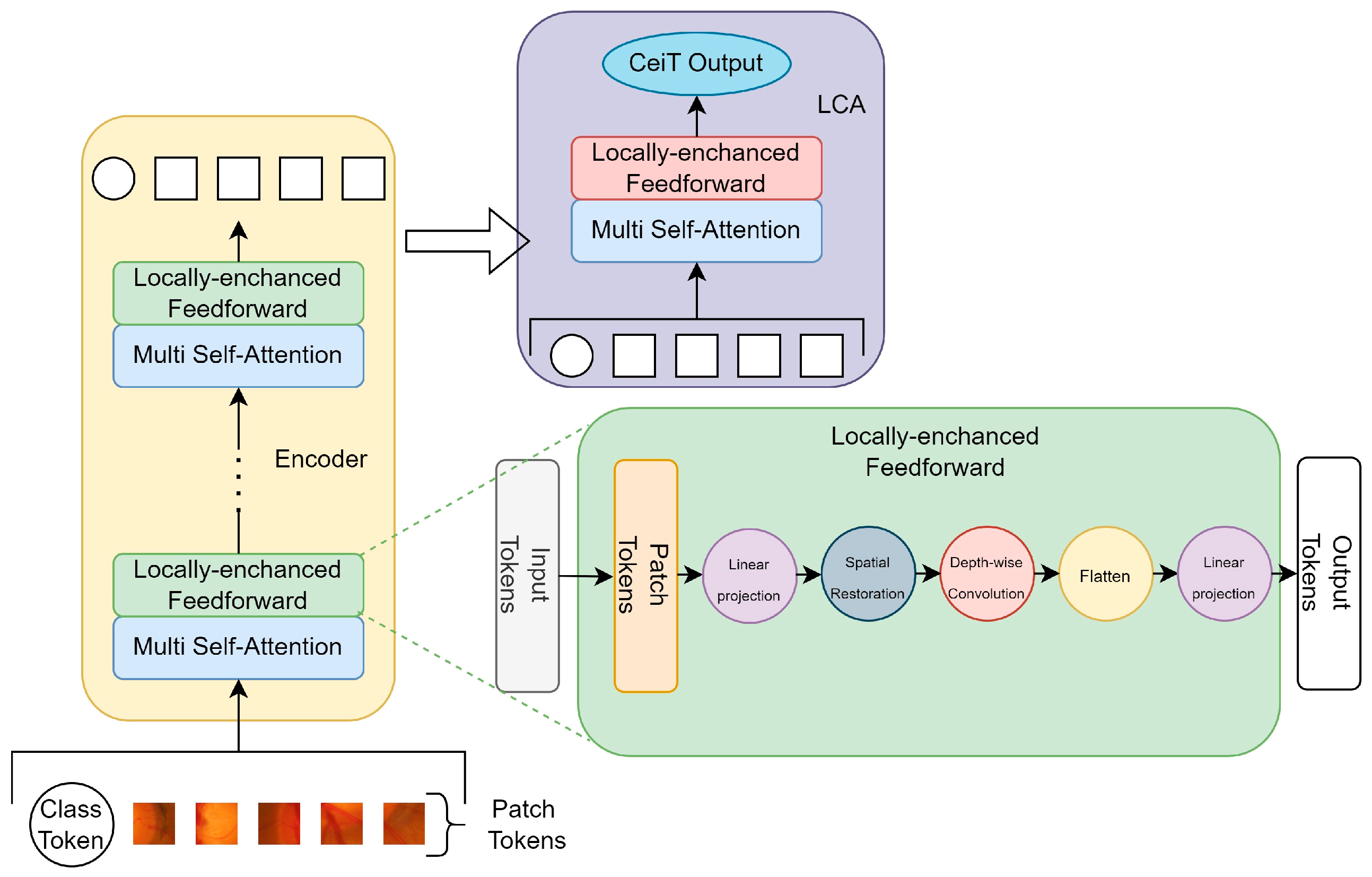
  • CeiT [28] incorporates several modifications over the original ViT. Firstly, it uses a low-level feature extraction module (image-to-token) that is applied to the input image. In the encoder blocks, the Feed-Forward Network (FFN) is replaced with a Locally Enhanced Feed-Forward Network (LeFF), which promotes correlation between tokens with convolution operations (Figure 12). Finally, a new type of block called “Layer-wise Class Token Attention” (LCA) is added, which contains a Multi Self-Attention MSA layer and an FFN. Its mission is to compute attention only on the class token, thus reducing the computational cost;
  • ConViT [29] introduces a new attention network called “gated positional self-attention” (GPSA). This network consists of a subnetwork that mimics convolutional behaviour and an attention head. There is a parameter that regulates the influence of both parts (Figure 13).

2.2.4. Other Architectures Inspired by Vision Transformers

In this section, we will focus on the ResMLP neural network [37], which is inspired by ViTs. The model follows the same distribution of layers and operations as ViTs, as well as working with the image divided into patches. However, it cannot be considered a ViT variant as it does not include the characteristic ViT attention mechanisms. Instead of attention layers, it uses linear Multi-Layer Perceptron (MLP) layers and non-linear Gaussian Error Linear Unit (GELU) layers. It also replaces the normalisation of the layers with a transformation that only shifts and rescales the input elements (“affine” blocks in Figure 14).
In the study presented in this article, two versions of this model of different sizes have been tested: “ResMLP_12” with 15 million parameters and “ResMLPB_24” with 129 million parameters.

2.3. Design of the Experiments

In this section, we describe the experimental methodology followed in the comparative study: how the training and test sets were designed with the available data, the training strategy, and the parameters selected for each model. We have tried to design an experimental framework that is as similar as possible for all models so that their efficiency results can be comparable.
For the training of all models used in this work, the initial set of 739 images was randomly divided into training and test sets with a ratio of 80/20, respectively.
  • Training set: 290 retinographies of glaucoma and 301 of healthy eyes;
  • Test set: 73 glaucoma retinographies and 75 healthy eyes.
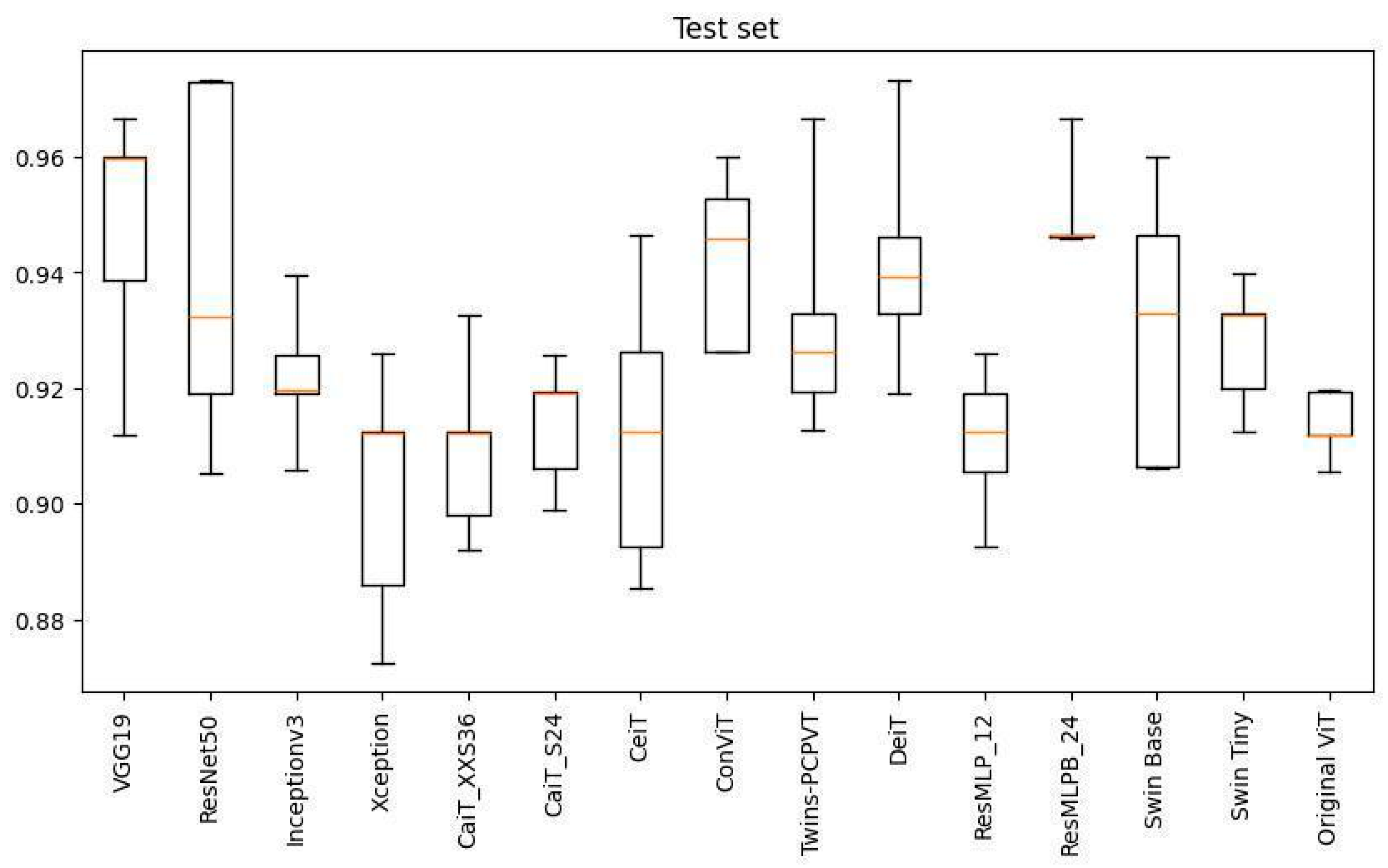
The training set was further divided into five different training and validation sets following a 5-fold approach.
The selected CNN models (VGG19, ResNet50, InceptionV3, and Xception) are available in the Keras module of the Tensorflow v2 package [47]. To adapt these neural network models to our classification problem, we replaced the top layer of each network with a DropOut layer, followed by a Flatten layer, followed by a Dense layer with 128 neurons with RELU activation, followed by a DropOut layer, and finally, a Dense layer with two outputs using the SoftMax activation function. This modification to the original CNNs’ architectures has been made because we have found in previous works that it improves the classification efficiency of the CNNs. For VGG19, the DropOut was set to 0.5. For InceptionV3, ResNet50, and Xception, the DropOut was set to 0.2. As for the size of the input layer, it was set to 224 × 224 × 3 for ResNet50 and VGG19 and 299 × 299 × 3 for InceptionV3 and Xception.
Our training strategy is the same for all CNN models. First, starting from the pre-trained ImageNet weights, we freeze the base model and train the new top layer for 200 epochs using an Adam optimiser, with a learning rate of 1e-6 and categorical cross-entropy as a loss function (fine tuning). Second, we unfroze the base model and trained the entire model end-to-end for 250 epochs using the same optimiser, with a learning rate of 10−5 and the same loss function as before (deep tuning). In all cases, a batch size of 8 was used.
Regarding the pre-processing step, we applied the pre-processing function included in Keras to each of the networks. To avoid overfitting, we applied data augmentation to the input samples, consisting of random contrast with a factor of +/− ±0.3, random brightness with a factor of ±0.3, random horizontal flip, random rotation ±45° with “nearest” fill mode, random horizontal and vertical translation with a factor of ±0.05 with “nearest” fill mode, and random zoom with a factor of ±0.2 preserving the aspect ratio with “nearest” fill mode.
The final weights for each model were chosen from the epoch that maximised the validation accuracy among the five folds. This results in 5 different models per CNN architecture, or 20 models in total.
On the other hand, the original ViT model is integrated into the Torchvision library of Pytorch [48]. The rest of the ViT models, hybrid systems, and ResMLP network have been obtained from the GitHub of the research groups that created them: CaiT, DeiT, and ResMLP from [49], CeiT from [50], the Swin models from [51], Twins-PCPVT from [52], and ConViT from [53].
We have retained the original architecture of each model, modifying only the last layer to adapt it to our two-class classification problem. For this reason, we replaced the top layer with a dense layer with two outputs. Regarding the DropOut, we have not added additional layers, and it is only used in the models that already have it integrated with its default values. Regarding the size of the input layer, it was set to 224 × 224 × 3 for all models.
As the original architecture of these models was not modified in any way (except for the last layer), all models were directly deep-tuned. Starting with the pre-trained weights from ImageNet, we trained the entire model end-to-end for 50 epochs using the Adam optimizer, with a learning rate of 10−5 and the categorical cross-entropy loss function. The value of 50 epochs was set empirically, as we observed in all tests the worsening behaviour of the models as training continued. Batch size was variable depending on what was allowed in each model: 32 for CaiT_XXS36, DeiT, ResMLP_12, CeiT, Swin Base, Swin Tiny, and Twins-PCPVT, 16 for CaiT_S24 and ConViT, and 4 for ResMLPB_24.
In the pre-processing step, we applied the pre-processing functions included in the library Torchvision of Pytorch [48]. To avoid overfitting, we applied data augmentation to the input samples, consisting of random brightness with a factor of ±0.5, random horizontal flip, random rotation ±15° with “nearest” fill mode, and normalisation.
Also, for these models, the final weights for each one were chosen from the epoch that maximised the validation accuracy among the five folds. This results in 5 different models per ViT-based system architecture, or 55 models in total.
All the trained DL models were tested with an independent set (test set) consisting of 75 samples from healthy subjects and 73 samples from glaucoma subjects. Subsequently, all these models were applied to other external retinography sets: the Drishti-GS1 database [45], the Papila dataset [46], and the REFUGE challenge database [44] to perform a more objective and comprehensive validation of their behaviour. The performance results corresponding to each network architecture are calculated in terms of sensitivity, specificity, accuracy, balanced accuracy, and F1 score [54].

3. Results

All the models were trained under the conditions described above and tested first with an independent set consisting of 75 samples from healthy subjects and 73 samples from glaucoma subjects (test set). The results corresponding to the best and worst performance, per architecture, in terms of balanced accuracy have been included in Table 1. Table 2, Table 3 and Table 4 show the results obtained by evaluating the different network models on REFUGE, Drishti-GS1, and Papila as test sets. Table 5 shows a ranking of the five models with the best-balanced accuracy in the classification of each dataset.

4. Discussion

The results of Table 1, Table 2, Table 3 and Table 4 clearly show that all architectures present the highest performance when classifying the images of the test set (Table 1). For this set, most of the trained models of each architecture have a balanced accuracy exceeding 90%. Such optimal results are not repeated when the set of retinographies to be classified changes. For example, in the case of Refuge, the best models classify with a balanced accuracy of around 83–89% (Table 2). In Drishti-GS1, the best results are in the range of 78–85% (Table 3), and in Papila, the most efficient models present a balanced accuracy of 74–80% (Table 4). These results are quite logical, considering that the test set belongs to the same set of images with which the DL models were trained, while the other three sets are different. Although these datasets are also composed of retinographies of healthy and glaucoma eyes, the images have been acquired with other cameras, under other conditions, and have been diagnosed by different medical experts. Another important factor to consider is that these external datasets are unbalanced, which is why we are using the balanced accuracy measure as a reference in our comparison.
Table 5 shows a ranking of the five models with the best-balanced accuracy in the classification of each dataset. It is interesting to note that, for all the datasets, the best model found is some type of CNN. However, the difference in efficiency with the second-ranked models, where some hybrid methods already appear, is very small. There are no significant differences between the best CNNs and ViT-based models when classifying the different datasets considered.
To study the variability of the five trained models of each architecture when performing the same classification task, we have plotted their balanced accuracy values in a Boxplot for each dataset: test set (Figure 15), Refuge dataset (Figure 16), Drishti-GS1 dataset (Figure 17), and Papila dataset (Figure 18).
In the case of the test set classification (Figure 15), the architecture with the lowest efficiency variability is ResMLPB_24. Of the five ResMLPB_24 models, four have a balanced accuracy of around 94%. On the other hand, the architecture ResNet50, previously presented as the best for classifying the test set (ranked 1st in Table 5), is the one with the highest balanced accuracy variability among its five trained models. Another interesting observation is that the VGG19 architecture is the one with the highest median value. This might lead us to think that this architecture may perform globally better for classifying the test set; however, it is the last to appear for this task in Table 5.
With the Refuge dataset, the architecture with the lowest balanced accuracy variability continues to be ResMLPB_24 (Figure 16). There are other architectures that present low variability as well but with worse balanced accuracy values (e.g., DeiT and VGG19). ResMLPB_24 is also the architecture that presents the highest median value, but it is ranked 4th in the ranking (Table 5). On the other hand, the CaiT_XXS36 architecture presents the highest variability with the worst efficiency values. It is interesting to note that by increasing the depth of this model and using its more complex version, CaiT_S24, both aspects improve notably.
In the Drishti-GS1 dataset classification, the architecture with the lowest balanced accuracy variability is Xception, but its efficiency is not among the best. Taking both factors into account, perhaps VGG19 is more optimal since its variability is low and its balanced accuracy values are higher. Table 5 shows that the architecture with the model with the highest balanced accuracy value is ResNet50. This architecture, as shown in Figure 17, has a medium variability. The original ViT is the one with the highest variability in this classification problem.
The architecture with the lowest efficiency variability when classifying the Papila dataset is CaiT_XXS36, but its efficiency improves notably when, again, the deepest version of this model, CaiT_S24, is used (Figure 18). VGG19 and ResMLP_24 seem to behave globally in a similar way, with VGG19 being slightly superior. This coincides with what is recorded in the ranking presented in Table 5.
One thing that occurs in all cases is that the ResMLP_12 architecture tends to present significantly lower balanced accuracy values and much higher variability than its deeper version, ResMLPB_24, just as with the versions of CaiT and Swin selected. Therefore, it seems convenient to choose, within the same architecture, the deeper versions of the glaucoma problem addressed in this article. If we do not consider these simplified versions of the studied architectures, we can observe that CNNs and ViT-based architectures present a similar behavior when classifying retinographies.
Whenever a comparative study such as the one proposed in this article is presented, it is always interesting to analyse the similarities and differences with other related works published in the scientific literature. In our case, we have not found any work that follows the experimental methodology we have developed, consisting of training models of 15 different architectures (between CNNs and ViT-based systems) with the retinographies of two databases (RIM_ONE DL and private data) and testing them with public databases not used in training (Refuge, Papila, and Drishti-GS1).
In the Introduction Section, we have briefly described other related published works [14,15,16,17,35,36,39]. Some of them analyse and compare the efficiency of some architectures studied in our work, such as ResNet50 [15,16,36,39], VGG19 [16,36], Xception [36], ViT and Swin Transformer [35,36], DeiT, ResMLP, and CaiT [35]. However, the training and test conditions are significantly different. On the other hand, there are works that propose their own architectures, as in [15,17]. Regarding the datasets used in the training and testing stages, each work uses and combines them differently. Some datasets are public and match those used in our work, e.g., Drishti-GS1 [14,15,16,35,36], Rim-ONE DL or some of its earlier versions [16,35,36,39], and Refuge [35,36], but others are different and, in some cases, private (ACRIMA [14,35,39], ORIGA [14,17,35,39], SCES [17], HVD [14], OHTS [39], HRF [15,35], DRIONS-DB [15], LAG [35,39], ESPERANZA [16], ODIR 5K [35]). Taking all this into account, we will now compare our results with those of these works indicatively.
In [14], the authors use several retinography datasets to train and test three different types of CNNs (ResNet101, NasNet, and NasNet_large). None of these networks has been studied in our work, and the only dataset we have used in common is Drishti-GS1. Their best classification results on this dataset (accuracy 77.23–82.18%) are worse than those obtained by the CNN architectures used in our study (accuracy 79.21–88.12%).
A comparative study between three CNNs (GoogleNet, VGG, and ResNet50) and an ensemble model of these architectures is presented in [15]. The datasets used are, again, different from those used by us, except for Drishti-GS1. With the two CNN architectures we have in common, VGG and ResNet50, the authors of [15] achieve high accuracy values of 91.08% and 93.06%, respectively. In our experiments with this dataset, the best VGG19 model presented an accuracy value of 84.16%, and the best ResNet50 model presented an accuracy value of 88.12%. Our values are lower, but we have not included retinographies of this dataset in our training, as in [15].
In [16], five different CNN architectures are trained using the Rim-ONE base for fine-tuning and the ESPERANZA and Drishti-GS1 datasets for deep tuning and the subsequent test process. Of the five architectures, two are analysed in our work: VGG19 and ResNet50. The best-balanced accuracy value obtained in [16] with VGG19 is 87.48%, and with ResNet50, it is 85.08%. These values are very similar to those obtained by us in the classification of the Drishti-GS1 dataset: 85.14% with ResNet50 and 82.47% with VGG19.
A comparison between different CNNs (VGG19, VGG16, Xception, ResNet50, ConvNext) and ViT-based (original ViT, Swin Transformer) architectures is presented in [36]. The authors merge the Drishti-GS1, Refuge, and Rim-ONE datasets to train and test the models. The best accuracy values they found are the following: 93.2% with VGG19, 91.8% with Xception, 91.1% with ResNet50, 95.8% with ViT, and 91.8% with Swin Transformer. It can be observed that there are no very significant differences in the performance of CNNs and ViT-based systems, which is something that we have also found in our experiments. The results presented in [36] are similar to those obtained in our experiments with the test set. With Refuge, the results of the CNNs in [36] are slightly higher than those obtained by our CNNs, and the accuracy values of the ViT-based systems remain similar. With Drishti-GS1, our results are noticeably worse than those found in [36] for all models. This difference between accuracy values is logical since, in our study, the Refuge and Drishti-GS1 datasets have been used exclusively for testing, unlike [36], which uses them both to train and test the models.
In [35], a comparative study of the performance of eight architectures based on ViTs is presented, among which we highlight five that coincide with those analysed in our work: Swin Transformer, CaiT, DeiT, original ViT, and ResMLP. To train and test all the models, the authors merge nine different public and private datasets so that they manage to reach a very high number of samples for training. Therefore, they achieved very high accuracy values: 93.2% with Swin Transformer, 94.5% with CaiT, 88.0% with DeiT, 87.4% with original ViT, and 91.5% with ResMLP. It is difficult to compare these results with ours since our training set is much smaller. Even so, we find it important to highlight that the accuracy values presented in Table 1 (test set classification results) are similar and even higher in some cases.
Finally, in [39], ResNet50 is compared with DeiT. The experimental methodology followed in this work is similar to ours: the architectures are trained with a single dataset (OHTS) and tested with other different datasets (DIGS/ADAGES, ACRIMA, LAG, Rim-ONE, ORIGA). The authors found that the DeiT architecture generalises better than ResNet50 in all the experiments. However, in our study, ResNet50 is superior to DeiT in almost all experiments. This may be because, in both works, the datasets chosen for training and testing are different.

5. Conclusions

In this research work, we have carried out an exhaustive comparison between the efficiency of CNNs and the most recent ViT-based architectures for the detection of glaucoma with fundus images. We have observed in the scientific literature that ViT-based systems are increasingly being used to aid in the diagnosis of glaucoma. These new works defend the superiority of ViT-based architectures over previous CNNs without having carried out a detailed study to support this conclusion. Considering the importance of the application of these systems in medical diagnosis, we consider that an in-depth study such as the one presented in our work is necessary.
We have tried to include a wide number of CNNs and ViT-based systems to make the conclusions as substantiated as possible. We have also considered the inclusion of multiple datasets to improve the reliability of the study’s findings and contribute to a more complete understanding of the performance of each DL system. All this makes the present comparative study very extensive. We have made a special effort in the results and discussion sections to condense all the information into tables and graphs that are useful for comparing the efficiency of the different architectures.
As a general conclusion, we can observe that the performance is quite similar between CNNs and ViT-based systems in the test set. With other external test sets, especially with Drishti-GS1 and PAPILA, CNNs show higher generalisation capacity than ViT-based systems. This may be because the efficiency of ViT-based systems is highly dependent on the size of the training set. Perhaps if trained with more samples, ViT-based systems could become superior to CNNs. Therefore, we consider the size and composition of the datasets to be very important factors.
A major difficulty encountered in the preparation of this work has been the attempt to compare the results with other similar studies already published. There is no consensus on developing a similar experimental methodology to allow an accurate comparison of architectures. In addition, there is a scarcity of datasets, and the few that exist present great variability in the way images are acquired and diagnosed.

Author Contributions

Conceptualisation, S.A. and J.F.S.; methodology, S.A., J.H. and F.J.F.; software, J.H. and F.J.F.; validation, S.A., J.F.S. and T.D.-A.; formal analysis, S.A. and J.F.S.; writing, S.A. and J.H. All authors have read and agreed to the published version of the manuscript.

Funding

This research was funded by the Gobierno de Canarias, grant number TESIS2022010056.

Institutional Review Board Statement

This study was conducted in accordance with the Declaration of Helsinki and approved by the Research Ethics Committee of the Canary Islands University Hospital (CHUC_2023_41, 27 April 2023). Confidentiality of personal data was guaranteed.

Informed Consent Statement

Informed consent was obtained from all subjects involved in the study.

Data Availability Statement

Publicly available datasets were analysed in this study. These data can be found here: Rim-ONE DL dataset at https://github.com/miag-ull/rim-one-dl (accessed on 6 October 2023), Refuge dataset at https://paperswithcode.com/dataset/refuge-challenge (accessed on 6 October 2023), Drishti-GS1 dataset at http://cvit.iiit.ac.in/projects/mip/drishti-gs/mip-dataset2/Home.php (accessed on 6 October 2023), and Papila dataset at https://figshare.com/articles/dataset/PAPILA/14798004 (accessed on 6 October 2023). The dataset collected by the medical experts at the Canary Islands University Hospital is not available.

Conflicts of Interest

The authors declare no conflict of interest.

References

  1. Tham, Y.-C.; Li, X.; Wong, T.Y.; Quigley, H.A.; Aung, T.; Cheng, C.-Y. Global Prevalence of Glaucoma and Projections of Glaucoma Burden through 2040: A Systematic Review and Meta-Analysis. Ophthalmology 2014, 121, 2081–2090. [Google Scholar] [CrossRef]
  2. Weinreb, R.N.; Aung, T.; Medeiros, F.A. The Pathophysiology and Treatment of Glaucoma: A Review. JAMA 2014, 311, 1901–1911. [Google Scholar] [CrossRef] [PubMed]
  3. Bernardes, R.; Serranho, P.; Lobo, C. Digital Ocular Fundus Imaging: A Review. Ophthalmologica 2011, 226, 161–181. [Google Scholar] [CrossRef] [PubMed]
  4. Yamashita, R.; Nishio, M.; Do, R.K.G.; Togashi, K. Convolutional Neural Networks: An Overview and Application in Radiology. Insights Into Imaging 2018, 9, 611–629. [Google Scholar] [CrossRef] [PubMed]
  5. Torres, J. First Contact with Deep Learning: Practical Introduction with Keras; Independently Published: Barcelona, Spain, 2018; Available online: https://torres.ai/first-contact-deep-learning-practical-introduction-keras/ (accessed on 4 October 2023).
  6. Esteva, A.; Kuprel, B.; Novoa, R.A.; Ko, J.; Swetter, S.M.; Blau, H.M.; Thrun, S. Dermatologist-Level Classification of Skin Cancer with Deep Neural Networks. Nature 2017, 542, 115–118. [Google Scholar] [CrossRef] [PubMed]
  7. Anthimopoulos, M.; Christodoulidis, S.; Ebner, L.; Christe, A.; Mougiakakou, S. Lung Pattern Classification for Interstitial Lung Diseases Using a Deep Convolutional Neural Network. IEEE Trans. Med. Imaging 2016, 35, 1207–1216. [Google Scholar] [CrossRef] [PubMed]
  8. Acharya, U.R.; Oh, S.L.; Hagiwara, Y.; Tan, J.H.; Adam, M.; Gertych, A.; Tan, R.S. A Deep Convolutional Neural Network Model to Classify Heartbeats. Comput. Biol. Med. 2017, 89, 389–396. [Google Scholar] [CrossRef] [PubMed]
  9. Spanhol, F.A.; Oliveira, L.S.; Petitjean, C.; Heutte, L. Breast Cancer Histopathological Image Classification Using Convolutional Neural Networks. In Proceedings of the 2016 International Joint Conference on Neural Networks (IJCNN), Vancouver, BC, Canada, 24 July 2016; pp. 2560–2567. [Google Scholar]
  10. Taormina, V.; Raso, G.; Gentile, V.; Abbene, L.; Buttacavoli, A.; Bonsignore, G.; Valenti, C.; Messina, P.; Scardina, G.A.; Cascio, D. Automated Stabilization, Enhancement and Capillaries Segmentation in Videocapillaroscopy. Sensors 2023, 23, 7674. [Google Scholar] [CrossRef]
  11. Wan, Z.; Wan, J.; Cheng, W.; Yu, J.; Yan, Y.; Tan, H.; Wu, J. A Wireless Sensor System for Diabetic Retinopathy Grading Using MobileViT-Plus and ResNet-Based Hybrid Deep Learning Framework. Appl. Sci. 2023, 13, 6569. [Google Scholar] [CrossRef]
  12. Gour, N.; Khanna, P. Multi-Class Multi-Label Ophthalmological Disease Detection Using Transfer Learning Based Convolutional Neural Network. Biomed. Signal Process. Control 2021, 66, 102329. [Google Scholar] [CrossRef]
  13. Simanjuntak, R.; Fu’adah, Y.; Magdalena, R.; Saidah, S.; Wiratama, A.; Ubaidah, I. Cataract Classification Based on Fundus Images Using Convolutional Neural Network. Int. J. Inform. Vis. 2022, 6, 33. [Google Scholar] [CrossRef]
  14. Velpula, V.K.; Sharma, L.D. Automatic Glaucoma Detection from Fundus Images Using Deep Convolutional Neural Networks and Exploring Networks Behaviour Using Visualization Techniques. SN Comput. Sci. 2023, 4, 487. [Google Scholar] [CrossRef]
  15. Joshi, S.; Partibane, B.; Hatamleh, W.A.; Tarazi, H.; Yadav, C.S.; Krah, D. Glaucoma Detection Using Image Processing and Supervised Learning for Classification. J. Healthc. Eng. 2022, 2022, 2988262. [Google Scholar] [CrossRef] [PubMed]
  16. Gómez-Valverde, J.J.; Antón, A.; Fatti, G.; Liefers, B.; Herranz, A.; Santos, A.; Sánchez, C.I.; Ledesma-Carbayo, M.J. Automatic Glaucoma Classification Using Color Fundus Images Based on Convolutional Neural Networks and Transfer Learning. Biomed. Opt. Express 2019, 10, 892–913. [Google Scholar] [CrossRef] [PubMed]
  17. Chen, X.; Xu, Y.; Wong, D.W.K.; Wong, T.Y.; Liu, J. Glaucoma Detection Based on Deep Convolutional Neural Network. In Proceedings of the 2015 37th Annual International Conference of the IEEE Engineering in Medicine and Biology Society (EMBC), Milan, Italy, 25–29 August 2015; pp. 715–718. [Google Scholar] [CrossRef]
  18. Simonyan, K.; Zisserman, A. Very Deep Convolutional Networks for Large-Scale Image Recognition. arXiv 2014, arXiv:1409.1556. [Google Scholar] [CrossRef]
  19. Vaswani, A.; Shazeer, N.; Parmar, N.; Uszkoreit, J.; Jones, L.; Gomez, A.N.; Kaiser, L.; Polosukhin, I. Attention Is All You Need. arXiv 2017, arXiv:1706.03762. [Google Scholar] [CrossRef]
  20. Dosovitskiy, A.; Beyer, L.; Kolesnikov, A.; Weissenborn, D.; Zhai, X.; Unterthiner, T.; Dehghani, M.; Minderer, M.; Heigold, G.; Gelly, S.; et al. An Image Is Worth 16x16 Words: Transformers for Image Recognition at Scale. arXiv 2020, arXiv:2010.11929. [Google Scholar] [CrossRef]
  21. Liu, Z.; Lin, Y.; Cao, Y.; Hu, H.; Wei, Y.; Zhang, Z.; Lin, S.; Guo, B. Swin Transformer: Hierarchical Vision Transformer Using Shifted Windows. In Proceedings of the IEEE/CVF International Conference on Computer Vision (ICCV), Montreal, BC, Canada, 11–17 October 2021; pp. 10012–10022. [Google Scholar] [CrossRef]
  22. Chu, X.; Tian, Z.; Wang, Y.; Zhang, B.; Ren, H.; Wei, X.; Xia, H.; Shen, C. Twins: Revisiting the Design of Spatial Attention in Vision Transformers. In Proceedings of the Advances in Neural Information Processing Systems 2021, Virtual, 6–14 December 2021; Volume 34, pp. 9355–9366. [Google Scholar] [CrossRef]
  23. Bazi, Y.; Bashmal, L.; Rahhal, M.M.A.; Dayil, R.A.; Ajlan, N.A. Vision Transformers for Remote Sensing Image Classification. Remote Sens. 2021, 13, 516. [Google Scholar] [CrossRef]
  24. Zheng, Y.; Jiang, W. Evaluation of Vision Transformers for Traffic Sign Classification. Wirel. Commun. Mob. Comput. 2022, 2022, 3041117. [Google Scholar] [CrossRef]
  25. Ghali, R.; Akhloufi, M.A.; Jmal, M.; Souidene Mseddi, W.; Attia, R. Wildfire Segmentation Using Deep Vision Transformers. Remote Sens. 2021, 13, 3527. [Google Scholar] [CrossRef]
  26. Touvron, H.; Cord, M.; Sablayrolles, A.; Synnaeve, G.; Jegou, H. Going Deeper with Image Transformers. In Proceedings of the 2021 IEEE/CVF International Conference on Computer Vision (ICCV), Montreal, BC, Canada, 11–17 October 2021; pp. 32–42. [Google Scholar] [CrossRef]
  27. Touvron, H.; Cord, M.; Douze, M.; Massa, F.; Sablayrolles, A.; Jegou, H. Training Data-Efficient Image Transformers & Distillation through Attention. In Proceedings of the 38th International Conference on Machine Learning, Virtual, 18–24 July 2021; Meila, M., Zhang, T., Eds.; Volume 139, pp. 10347–10357. [Google Scholar] [CrossRef]
  28. Yuan, K.; Guo, S.; Liu, Z.; Zhou, A.; Yu, F.; Wu, W. Incorporating Convolution Designs into Visual Transformers. In Proceedings of the 2021 IEEE/CVF International Conference on Computer Vision (ICCV), Montreal, BC, Canada, 11–17 October 2021; pp. 559–568. [Google Scholar] [CrossRef]
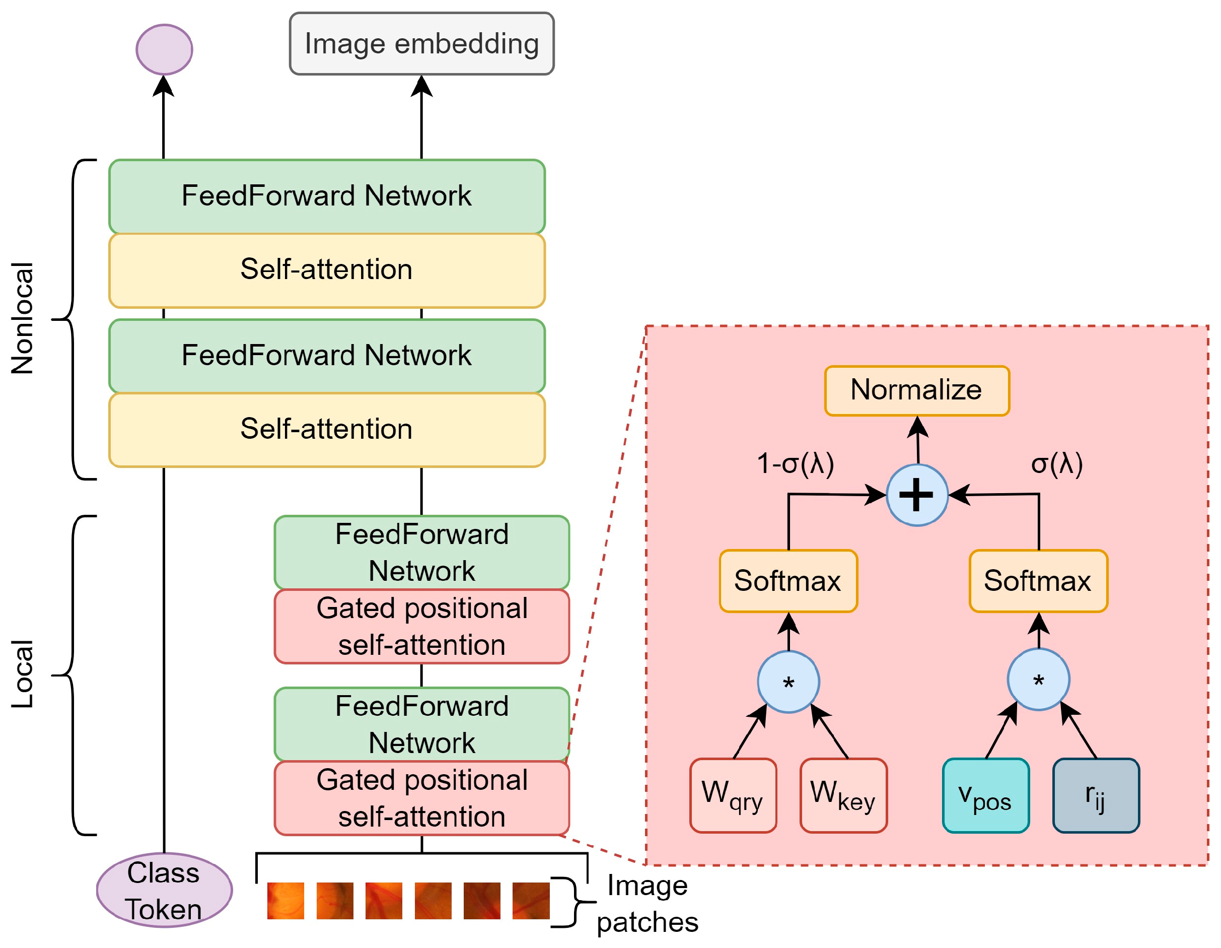
  29. d’Ascoli, S.; Touvron, H.; Leavitt, M.L.; Morcos, A.S.; Biroli, G.; Sagun, L. ConViT: Improving Vision Transformers with Soft Convolutional Inductive Biases. J. Stat. Mech. Theory Exp. 2022, 2022, 114005. [Google Scholar] [CrossRef]
  30. Rao, S.; Li, Y.; Ramakrishnan, R.; Hassaine, A.; Canoy, D.; Cleland, J.; Lukasiewicz, T.; Salimi-Khorshidi, G.; Rahimi, K. An Explainable Transformer-Based Deep Learning Model for the Prediction of Incident Heart Failure. IEEE J. Biomed. Health Inf. 2022, 26, 3362–3372. [Google Scholar] [CrossRef] [PubMed]
  31. Vaid, A.; Jiang, J.; Sawant, A.; Lerakis, S.; Argulian, E.; Ahuja, Y.; Lampert, J.; Charney, A.; Greenspan, H.; Narula, J.; et al. A Foundational Vision Transformer Improves Diagnostic Performance for Electrocardiograms. NPJ Digit. Med. 2023, 6, 108. [Google Scholar] [CrossRef] [PubMed]
  32. Nerella, S.; Bandyopadhyay, S.; Zhang, J.; Contreras, M.; Siegel, S.; Bumin, A.; Silva, B.; Sena, J.; Shickel, B.; Bihorac, A.; et al. Transformers in Healthcare: A Survey. arXiv 2023, arXiv:2307.00067. [Google Scholar]
  33. Mohan, N.J.; Murugan, R.; Goel, T.; Roy, P. ViT-DR: Vision Transformers in Diabetic Retinopathy Grading Using Fundus Images. In Proceedings of the 2022 IEEE 10th Region 10 Humanitarian Technology Conference (R10-HTC), Hyderabad, India, 16–18 September 2022; pp. 167–172. [Google Scholar] [CrossRef]
  34. Jiang, Z.; Wang, L.; Wu, Q.; Shao, Y.; Shen, M.; Jiang, W.; Dai, C. Computer-Aided Diagnosis of Retinopathy Based on Vision Transformer. J. Innov. Opt. Health Sci. 2022, 15, 2250009. [Google Scholar] [CrossRef]
  35. Wassel, M.; Hamdi, A.M.; Adly, N.; Torki, M. Vision Transformers Based Classification for Glaucomatous Eye Condition. In Proceedings of the 2022 26th International Conference on Pattern Recognition (ICPR), Montreal, QC, Canada, 21–25 August 2022; pp. 5082–5088. [Google Scholar] [CrossRef]
  36. Mallick, S.; Paul, J.; Sengupta, N.; Sil, J. Study of Different Transformer Based Networks for Glaucoma Detection. In Proceedings of the TENCON 2022–2022 IEEE Region 10 Conference (TENCON), Hong Kong, 1–4 November 2022; pp. 1–6. [Google Scholar] [CrossRef]
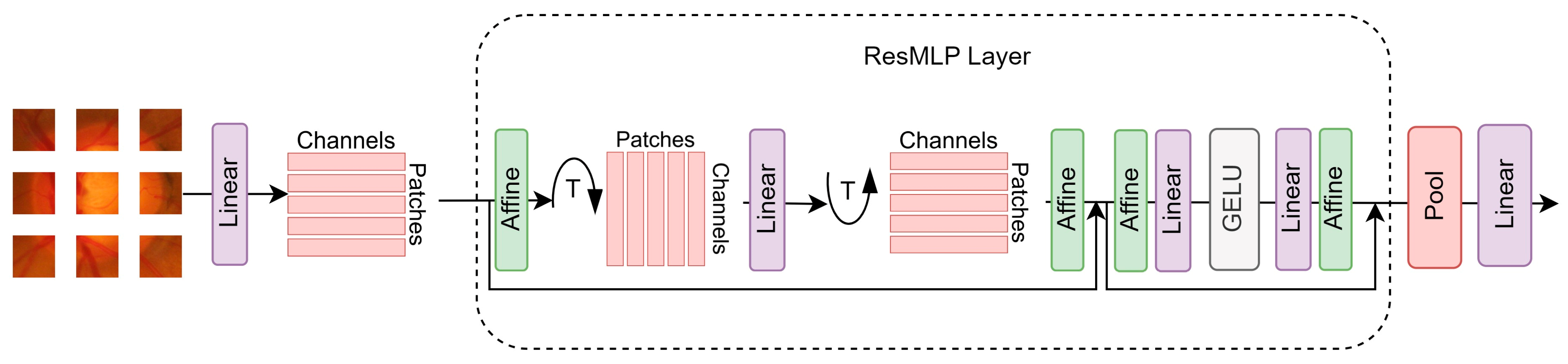
  37. Touvron, H.; Bojanowski, P.; Caron, M.; Cord, M.; El-Nouby, A.; Grave, E.; Izacard, G.; Joulin, A.; Synnaeve, G.; Verbeek, J.; et al. ResMLP: Feedforward Networks for Image Classification with Data-Efficient Training. IEEE Trans. Pattern Anal. Mach. Intell. 2023, 45, 5314–5321. [Google Scholar] [CrossRef]
  38. Maurício, J.; Domingues, I.; Bernardino, J. Comparing Vision Transformers and Convolutional Neural Networks for Image Classification: A Literature Review. Appl. Sci. 2023, 13, 5521. [Google Scholar] [CrossRef]
  39. Fan, R.; Alipour, K.; Bowd, C.; Christopher, M.; Brye, N.; Proudfoot, J.A.; Goldbaum, M.H.; Belghith, A.; Girkin, C.A.; Fazio, M.A.; et al. Detecting Glaucoma from Fundus Photographs Using Deep Learning without Convolutions: Transformer for Improved Generalization. Ophthalmol. Sci. 2023, 3, 100233. [Google Scholar] [CrossRef]
  40. He, K.; Zhang, X.; Ren, S.; Sun, J. Deep Residual Learning for Image Recognition. In Proceedings of the 2016 IEEE Conference on Computer Vision and Pattern Recognition (CVPR), Las Vegas, NV, USA, 27–30 June 2016; pp. 770–778. [Google Scholar] [CrossRef]
  41. Szegedy, C.; Vanhoucke, V.; Ioffe, S.; Shlens, J.; Wojna, Z. Rethinking the Inception Architecture for Computer Vision. In Proceedings of the 2016 IEEE Conference on Computer Vision and Pattern Recognition (CVPR), Las Vegas, NV, USA, 27–30 June 2016; IEEE Computer Society: Los Alamitos, CA, USA, 2016; pp. 2818–2826. [Google Scholar] [CrossRef]
  42. Chollet, F. Xception: Deep Learning with Depthwise Separable Convolutions. In Proceedings of the 2017 IEEE Conference on Computer Vision and Pattern Recognition (CVPR), Honolulu, HI, USA, 21–26 July 2017; IEEE Computer Society: Los Alamitos, CA, USA, 2017; pp. 1800–1807. [Google Scholar] [CrossRef]
  43. Fumero Batista, F.J.; Diaz-Aleman, T.; Sigut, J.; Alayon, S.; Arnay, R.; Angel-Pereira, D. RIM-ONE DL: A Unified Retinal Image Database for Assessing Glaucoma Using Deep Learning. Image Anal. Stereol. 2020, 39, 161–167. [Google Scholar] [CrossRef]
  44. Orlando, J.I.; Fu, H.; Breda, J.B.; van Keer, K.; Bathula, D.R.; Diaz-Pinto, A.; Fang, R.; Heng, P.-A.; Kim, J.; Lee, J.; et al. REFUGE Challenge: A Unified Framework for Evaluating Automated Methods for Glaucoma Assessment from Fundus Photographs. Med. Image Anal. 2020, 59, 101570. [Google Scholar] [CrossRef]
  45. Sivaswamy, J.; Krishnadas, S.R.; Datt Joshi, G.; Jain, M.; Syed Tabish, A.U. Drishti-GS: Retinal Image Dataset for Optic Nerve Head(ONH) Segmentation. In Proceedings of the 2014 IEEE 11th International Symposium on Biomedical Imaging (ISBI), Beijing, China, 29 April–2 May 2014; pp. 53–56. [Google Scholar] [CrossRef]
  46. Kovalyk, O.; Morales-Sánchez, J.; Verdú-Monedero, R.; Sellés-Navarro, I.; Palazón-Cabanes, A.; Sancho-Gómez, J.-L. PAPILA: Dataset with Fundus Images and Clinical Data of Both Eyes of the Same Patient for Glaucoma Assessment. Sci. Data 2022, 9, 291. [Google Scholar] [CrossRef] [PubMed]
  47. Abadi, M.; Agarwal, A.; Barham, P.; Brevdo, E.; Chen, Z.; Citro, C.; Corrado, G.S.; Davis, A.; Dean, J.; Devin, M.; et al. TensorFlow: Large-Scale Machine Learning on Heterogeneous Distributed Systems. arXiv 2016, arXiv:1603.04467. Available online: www.tensorflow.org (accessed on 4 October 2023).
  48. TorchVision—TorchVision 0.15 Documentation. Available online: https://pytorch.org/vision/stable/index.html (accessed on 4 October 2023).
  49. DeiT GitHub from the Meta Research Group. Available online: https://github.com/facebookresearch/deit (accessed on 4 October 2023).
  50. GitHub of the Hong Kong University of Science and Technology. Available online: https://github.com/coeusguo/ceit (accessed on 4 October 2023).
  51. GitHub of the Microsoft Group. Available online: https://github.com/microsoft/Swin-Transformer (accessed on 4 October 2023).
  52. GitHub of the Meituan-AutoML Group. Available online: https://github.com/Meituan-AutoML/Twins (accessed on 4 October 2023).
  53. ConViT GitHub from the Meta Research Group. Available online: https://github.com/facebookresearch/convit (accessed on 4 October 2023).
  54. Brzezinski, D.; Stefanowski, J.; Susmaga, R.; Szczȩch, I. Visual-Based Analysis of Classification Measures and Their Properties for Class Imbalanced Problems. Inf. Sci. 2018, 462, 242–261. [Google Scholar] [CrossRef]
Figure 1. Eye fundus image with localised optic disc and optic cup.
Applsci 13 12722 g001
Figure 2. Architecture of VGG19.
Applsci 13 12722 g002
Figure 3. Architecture of ResNet50.
Applsci 13 12722 g003
Figure 4. Architecture of InceptionV3.
Applsci 13 12722 g004
Figure 5. Architecture of Xception.
Applsci 13 12722 g005
Figure 6. Encoder–Decoder architecture of a Transformer. Image extracted from [19].
Applsci 13 12722 g006
Figure 7. ViT model overview.
Applsci 13 12722 g007
Figure 8. Differences between Swin Transformer and ViT. Image extracted from [21].
Applsci 13 12722 g008
Figure 9. Architecture of Twins-PCPVT.
Applsci 13 12722 g009
Figure 10. Architecture of DeiT.
Applsci 13 12722 g010
Figure 11. Architecture of CaiT.
Applsci 13 12722 g011
Figure 12. Architecture of CeiT.
Applsci 13 12722 g012
Figure 13. Architecture of ConViT.
Applsci 13 12722 g013
Figure 14. Architecture of ResMLP.
Applsci 13 12722 g014
Figure 15. Boxplot of the balanced accuracy values of the five models of each architecture when classifying the test set: minimum value, maximum value, median, and quartiles 1 and 3.
Applsci 13 12722 g015
Figure 16. Boxplot of the balanced accuracy values of the five models of each architecture when classifying the Refuge dataset: minimum value, maximum value, median, and quartiles 1 and 3.
Applsci 13 12722 g016
Figure 17. Boxplot of the balanced accuracy values of the five models of each architecture when classifying the Drishti-GS1 dataset: minimum value, maximum value, median, and quartiles 1 and 3.
Applsci 13 12722 g017
Figure 18. Boxplot of the balanced accuracy values of the five models of each architecture when classifying the Papila dataset: minimum value, maximum value, median, and quartiles 1 and 3.
Applsci 13 12722 g018
Table 1. Summary of the results obtained by evaluating the different DL models on the test dataset according to different metrics. For simplicity, only the results corresponding to the folds with minimum and maximum balanced accuracy (B. Accuracy) are displayed.
ArchitectureFoldSensitivitySpecificityAccuracyB. AccuracyF1 Score
CNNsVGG19fold_10.87670.94670.91220.91170.9078
VGG19fold_40.98630.94670.96620.96650.9664
ResNet50fold_10.93150.90670.91890.91910.9189
ResNet50fold_30.98630.96000.97300.97320.9730
InceptionV3fold_20.94520.86670.90540.90590.9079
InceptionV3fold_30.97260.90670.93920.93960.9404
Xceptionfold_50.93150.81330.87160.87240.8774
Xceptionfold_10.94520.90670.92570.92590.9262
ViTsOriginal ViTfold_50.91780.89330.90540.90560.9054
Original ViTfold_40.97260.86670.91890.91960.9221
Swin Basefold_50.94520.86670.90540.90590.9079
Swin Basefold_10.98630.93330.95950.95980.9600
Swin Tinyfold_10.93150.89330.91220.91240.9128
Swin Tinyfold_20.98630.89330.93920.93980.9412
Twins-PCPVTfold_30.94520.88000.91220.91260.9139
Twins-PCPVTfold_21.00000.93330.96620.96670.9669
Hybrid modelsDeiTfold_50.91780.92000.91890.91890.9178
DeiTfold_40.98630.96000.97300.97320.9730
CaiT_XXS36fold_10.90410.88000.89190.89210.8919
CaiT_XXS36fold_40.93150.93330.93240.93240.9315
CaiT_S24fold_20.91780.88000.89860.89890.8993
CaiT_S24fold_40.91780.93330.92570.92560.9241
CeiTfold_30.90410.86670.88510.88540.8859
CeiTfold_20.98630.90670.94590.94650.9474
ConViTfold_30.95890.89330.92570.92610.9272
ConViTfold_50.98630.93330.95950.95980.9600
Others inspired in ViTResMLP_12fold_30.93150.85330.89190.89240.8947
ResMLP_12fold_10.94520.90670.92570.92590.9262
ResMLPB_24fold_10.94520.94670.94590.94590.9452
ResMLPB_24fold_50.98630.94670.96620.96650.9664
Table 2. Summary of the results obtained by evaluating the different DL models on the Refuge dataset according to different metrics. For simplicity, only the results corresponding to the folds with minimum and maximum balanced accuracy (B. Accuracy) are displayed.
ArchitectureFoldSensitivitySpecificityAccuracyB. AccuracyF1 Score
CNNsVGG19fold_40.78330.85370.84670.81850.5054
VGG19fold_50.88330.88980.88920.88660.6145
ResNet50fold_50.80830.80650.80670.80740.4554
ResNet50fold_20.84170.90090.89500.87130.6159
InceptionV3fold_40.67500.98430.95330.82960.7431
InceptionV3fold_30.85000.93890.93000.89440.7083
Xceptionfold_50.92500.68980.71330.80740.3922
Xceptionfold_20.80830.89630.88750.85230.5897
ViTsOriginal ViTfold_10.70000.96670.94000.83330.7000
Original ViTfold_40.81670.93430.92250.87550.6782
Swin Basefold_20.68330.93890.91330.81110.6119
Swin Basefold_50.81670.91940.90920.86810.6426
Swin Tinyfold_10.55000.94540.90580.74770.5388
Swin Tinyfold_20.76670.93150.91500.84910.6434
Twins-PCPVTfold_40.77500.85460.84670.81480.5027
Twins-PCPVTfold_20.84170.87130.86830.85650.5611
Hybrid modelsDeiTfold_50.74170.93700.91750.83940.6426
DeiTfold_40.78330.93520.92000.85930.6620
CaiT_XXS36fold_30.50000.97410.92670.73700.5769
CaiT_XXS36fold_50.79170.90830.89670.85000.6051
CaiT_S24fold_30.70830.94170.91830.82500.6343
CaiT_S24fold_10.83330.90090.89420.86710.6116
CeiTfold_30.68330.84810.83170.76570.4481
CeiTfold_40.79170.89350.88330.84260.5758
ConViTfold_10.62500.96670.93250.79580.6494
ConViTfold_20.83330.94350.93250.88840.7117
Others inspired in ViTResMLP_12fold_40.64170.87500.85170.75830.4639
ResMLP_12fold_10.83330.82960.83000.83150.4950
ResMLPB_24fold_20.72500.98330.95750.85420.7733
ResMLPB_24fold_30.83330.93800.92750.88560.6969
Table 3. Summary of the results obtained by evaluating the different DL models on the Drishti-Gs1 dataset according to different metrics. For simplicity, only the results corresponding to the folds with minimum and maximum balanced accuracy (B. Accuracy) are displayed.
ArchitectureFoldSensitivitySpecificityAccuracyB. AccuracyF1 Score
CNNsVGG19fold_40.88570.74190.84160.81380.8857
VGG19fold_30.84290.80650.83170.82470.8741
ResNet50fold_30.81430.74190.79210.77810.8444
ResNet50fold_10.92860.77420.88120.85140.9155
InceptionV3fold_20.85710.74190.82180.79950.8696
InceptionV3fold_50.88570.77420.85150.83000.8921
Xceptionfold_20.87140.67740.81190.77440.8652
Xceptionfold_30.82860.74190.80200.78530.8529
ViTsOriginal ViTfold_20.54290.90320.65350.72300.6847
Original ViTfold_30.78570.83870.80200.81220.8462
Swin Basefold_20.64290.80650.69310.72470.7438
Swin Basefold_50.87140.77420.84160.82280.8841
Swin Tinyfold_20.68570.83870.73270.76220.7805
Swin Tinyfold_30.80000.80650.80200.80320.8485
Twins-PCPVTfold_30.65710.80650.70300.73180.7541
Twins-PCPVTfold_20.90000.67740.83170.78870.8811
Hybrid modelsDeiTfold_20.62860.87100.70300.74980.7458
DeiTfold_50.84290.74190.81190.79240.8613
CaiT_XXS36fold_30.60000.83870.67330.71940.7179
CaiT_XXS36fold_10.75710.90320.80200.83020.8413
CaiT_S24fold_40.67140.80650.71290.73890.7642
CaiT_S24fold_10.82860.80650.82180.81750.8657
CeiTfold_10.78570.67740.75250.73160.8148
CeiTfold_30.72860.83870.76240.78360.8095
ConViTfold_10.68570.80650.72280.74610.7742
ConViTfold_30.84290.77420.82180.80850.8676
Others inspired in ViTResMLP_12fold_30.52860.90320.64360.71590.6727
ResMLP_12fold_50.84290.80650.83170.82470.8741
ResMLPB_24fold_20.74290.77420.75250.75850.8062
ResMLPB_24fold_30.91430.74190.86140.82810.9014
Table 4. Summary of the results obtained by evaluating the different DL models on the Papila dataset according to different metrics. For simplicity, only the results corresponding to the folds with minimum and maximum balanced accuracy (B. Accuracy) are displayed.
ArchitectureFoldSensitivitySpecificityAccuracyB. AccuracyF1 Score
CNNsVGG19fold_50.78160.75380.75950.76770.5738
VGG19fold_20.75860.84380.82620.80120.6439
ResNet50fold_50.70110.78680.76900.74400.5571
ResNet50fold_20.71260.86790.83570.79030.6425
InceptionV3fold_20.82760.69070.71900.75910.5496
InceptionV3fold_10.79310.80180.80000.79750.6216
Xceptionfold_30.88510.63360.68570.75930.5385
Xceptionfold_10.79310.75380.76190.77340.5798
ViTsOriginal ViTfold_40.86210.50000.57480.68100.4559
Original ViTfold_50.81610.71260.73400.76430.5591
Swin Basefold_40.58620.79340.75060.68980.4928
Swin Basefold_10.73560.81740.80050.77650.6038
Swin Tinyfold_50.81610.60480.64850.71040.4897
Swin Tinyfold_40.73560.78140.77200.75850.5714
Twins-PCPVTfold_50.80460.52990.58670.66730.4459
Twins-PCPVTfold_30.77010.78440.78150.77730.5929
Hybrid modelsDeiTfold_50.79310.60480.64370.69890.4792
DeiTfold_40.65520.84430.80520.74970.5816
CaiT_XXS36fold_30.64370.82340.78620.73350.5545
CaiT_XXS36fold_10.72410.78140.76960.75280.5650
CaiT_S24fold_40.64370.83530.79570.73950.5657
CaiT_S24fold_10.77010.80540.79810.78780.6119
CeiTfold_40.71260.72460.72210.71860.5145
CeiTfold_50.77010.80540.79810.78780.6119
ConViTfold_50.79310.63170.66510.71240.4946
ConViTfold_10.74710.73050.73400.73880.5372
Others inspired in ViTResMLP_12fold_40.60920.76050.72920.68480.4818
ResMLP_12fold_10.58620.89220.82900.73920.5862
ResMLPB_24fold_40.71260.79640.77910.75450.5714
ResMLPB_24fold_50.72410.86830.83850.79620.6495
Table 5. Summary of the top five models for each dataset and their values of balanced accuracy.
Ranking PositionTest Set RefugeDrishti-GS1Papila
1ResNet50
97.32%
InceptionV3
89.44%
ResNet50
85.14%
VGG19
80.12%
2DeiT
97.32%
ConViT
88.84%
CaiT_XXS36
83.02%
InceptionV3
79.75%
3Twins-PCPVT
96.67%
VGG19
88.66%
InceptionV3
83.00%
ResMLPB_24
79.62%
4ResMLPB_24
96.65%
ResMLPB_24
88.56%
ResMLPB_24
82.81%
ResNet50
79.03%
5VGG19
96.65%
Original ViT
87.55%
VGG19
82.47%
CaiT_S24
78.78%
Disclaimer/Publisher’s Note: The statements, opinions and data contained in all publications are solely those of the individual author(s) and contributor(s) and not of MDPI and/or the editor(s). MDPI and/or the editor(s) disclaim responsibility for any injury to people or property resulting from any ideas, methods, instructions or products referred to in the content.

